Stellar disruption events support the existence of the black hole event horizon

Abstract

Many black hole (BH) candidates have been discovered in X-ray binaries and in the nuclei of galaxies. The prediction of Einstein’s general relativity is that BHs have an event horizon — a one-way membrane through which particles fall into the BH but cannot exit. However, except for the very few nearby supermassive BH candidates, our telescopes are unable to resolve and provide a direct proof of the event horizon. Here, we propose a novel observation that supports the existence of event horizons around supermassive BH candidates heavier than $10^{7.5}M_{\rm\odot}$. Instead of an event horizon, if the BH candidate has a hard surface, when a star falls onto the surface, the shocked baryonic gas will form a radiation pressure supported envelope that shines at the Eddington luminosity for an extended period of time from months to years. We show that such emission has already been ruled out by the Pan-STARRS1 3$\pi$ survey if supermassive BH candidates have a hard surface at radius larger than $(1+10^{-4.4})$ times the Schwarzschild radius. Future observations by LSST should be able to improve the limit to $1+10^{-6}$.

1 Introduction

A black hole (BH) forms when no other force can uphold gravity and everything collapses down to a point of roughly Planck size $\sim 10^{-33}\rm\ cm$. The prediction of Einstein’s general relativity is that the point mass must be enclosed inside an event horizon, through which matter, energy and light can enter from outside, but nothing can exit. For a non-spinning BH, the size of the event horizon, or the Schwarzschild radius, is proportional to the mass $M=10^{7}M_{7}M_{\rm\odot}$ as

$$r_{\rm S}\equiv\frac{2GM}{c^{2}}=3.0\times 10^{12}M_{7}\rm\ cm.$$ (1)

Over the past 30 years, BH candidates have been found and classified according to their masses, with stellar-mass candidates having a few up to tens of $M_{\rm\odot}$ and supermassive candidates with masses $\sim 10^{6}$-$10^{10}M_{\rm\odot}$. Proving the existence of the defining characteristic of BHs — the event horizon — would provide crucial support for Einstein’s general relativity. However, BH event horizons are usually too small for our telescopes to resolve.

Nearly all galaxies have a central massive object (CMO) of mass $\sim 10^{6}$-$10^{10}M_{\rm\odot}$ (e.g. Kormendy & Ho, 2013). The nature of the CMOs is important in many astrophysical fields, e.g. active galactic nuclei, galaxy evolution, gravitational wave, etc. CMOs are widely believed to be BHs, due to the following reasons (many of which have been discussed by Narayan & McClintock, 2008).

(1) If the mass of a compact object exceeds the maximum neutron star mass $M_{\rm NS,max}\sim 3M_{\odot}$, there is no known force that can hold it up from collapsing. (2) Since active galactic nuclei are powered by accretion (or gravitational potential energy), the central mass-gaining object or cluster is expected to undergo collapse and eventually turn into a BH, if there is no exotic force supporting gravity (e.g. Rees, 1984). (3) In the absence of an event horizon, the kinetic energy of the infalling gas will be converted into radiation inside or on the surface of the CMO. For the two nearby CMOs at the centers of the Milky Way and M87 (Sgr A* and M87*), if they do not have event horizons and are in thermal dynamic equilibrium, this amount of radiation ($\sim\dot{M}c^{2}$) overproduces the observed infrared flux by a factor of 10–100 (Broderick et al., 2009, 2015). (4) The Event Horizon Telescope (EHT) images of Sgr A* and M87* in the millimeter wavelength so far are consistent with a point source of radius $\lesssim 2$-$2.5r_{\rm S}$ (Doeleman et al., 2008, 2012), which roughly corresponds to the apparent size of the photon capture radius (“BH shadow”), so a hard surface at radius significantly larger than $1.5r_{\rm S}$ has been ruled out (Broderick & Narayan, 2006). As the sensitivity and resolution of EHT improve, future images will be compared to realistic accretion flow models and will directly test the spacetime metric. (5) The LIGO detections of gravitational wave bursts (e.g. GW150914) are consistent with merging stellar-mass BHs (Abbott et al., 2016).

While the reasons above are certainly strong, one may argue: reason (1) may not apply to CMOs because their compactness is unknown and there might be some mechanism/material that can support them from collapsing; reason (2) does not rule out many classes of BH alternative models either (e.g. boson stars and gravastars, Schunck & Mielke, 2003; Mazur & Mottola, 2004); reasons (3) and (4) apply to only a few nearby CMOs (due to our telescopes’ finite resolution). As for reason (5), gravitational wave generation calculations for binary merger events for alternative models of BHs (objects without event horizon) have only been done in the ringdown phase where the differences only appear in the late-time secondary pulses in the high-compactness limit (e.g. Yunes et al., 2016). Future work on the gravitational wave emission during the plunge and merger phase, combined with higher signal-to-noise ratio LIGO detections, will put better constraints on the alternative models.

In this paper, we propose a novel observation that places stringent constraints on the possible location of a hard surface around CMOs and hence strongly argues for them being BHs with event horizons.

2 The Idea

Stars can be driven into nearly radial orbits towards the CMO by different processes, e.g. two-body relaxation, resonant relaxation, massive perturbers, non-spherical potential (Alexander, 2005). If the CMO is compact enough, stars could reach down to a critical radius where the tidal gravity exceeds the star’s self-gravity, causing a tidal disruption event (TDE). The Newtonian tidal disruption radius is given by (e.g. Rees, 1988)

$$\frac{r_{\rm T}}{r_{\rm S}}\simeq 5.0r_{\rm*}m_{\rm*}^{-1/3}M_{7}^{-2/3},$$ (2)

where the star’s mass and radius are expressed in units of solar mass and solar radius, $M_{\rm*}=m_{\rm*}M_{\rm\odot}$ and $R_{\rm*}=r_{\rm*}R_{\rm\odot}$. When $M\gtrsim 10^{7.5}M_{\rm\odot}$, the Newtonian tidal disruption radius is not applicable and a full general relativistic treatment is necessary (e.g. Kesden, 2012; Servin & Kesden, 2016). When the star crosses $r_{\rm T}$, the tidal gravity of the CMO causes a spread of specific orbital energy across the star, which leaves roughly half of the star in bound orbits and the other half unbound. Then the fall-back gas forms a thick accretion disk which produces months-long optical/UV luminosity $10^{44}$-$10^{45}\rm\ erg/s$ observable at cosmological distances. Recently, a few dozen of such TDE candidates have been observed from various surveys carried out in the optical, UV and soft X-ray wavelengths, giving a TDE rate of $\sim 10^{-5}\rm\ yr^{-1}\ galaxy^{-1}$, consistent with but somewhat lower than theoretical estimates (see the review by Komossa, 2015).

The star in a TDE can be used as a test particle to probe the nature of the CMO, because it reaches very close to $r_{\rm S}$. In this paper, we consider the observational consequences of star-CMO close encounters if the CMO does not possess an event horizon. We assume the CMO’s radius to be

$$r_{0}=\eta r_{\rm S},$$ (3)

where $\eta>1$ is a free parameter. If the CMO has a hard surface, then $r_{0}$ is the surface radius; if the CMO is a diffuse cluster of non-luminous particles or objects, then $r_{0}$ is defined as the half-mass radius and $M$ is the mass enclosed within radius $r_{0}$. There are two possibilities in the hard-surface scenario (and both are considered in this paper): if the CMO is made of ordinary matter, the Buchdahl limit gives $\eta>9/8$ (Buchdahl, 1959); if exotic forces are allowed, $\eta$ can be extremely close to 1.

From eq. (2), we know that TDEs with accretion disk formation are only possible if the radius of the CMO is smaller than $r_{\rm T}$, i.e.

$$\eta M_{7}^{2/3}<5.0r_{\rm*}m_{\rm*}^{-1/3}.$$ (4)

Therefore, considering the fact that TDEs from CMOs of roughly $10^{6}M_{\rm\odot}$ have been observed, we obtain an upper limit $\eta<30$. The nature of CMOs should not depend on their masses, so we only consider the parameter space $1<\eta<30$. The upper limit on $\eta$ can rule out CMOs being clusters of brown dwarfs or stellar remnants (white dwarfs, neutron stars and stellar-mass BHs), because the lifetime due to collisions or evaporation is much shorter than $10\rm\ Gyr$ (Maoz, 1998). Other alternative models cannot be ruled out yet, such as objects with a hard surface supported by exotic forces (e.g. gravastars, Mazur & Mottola, 2004) or the configuration from collapse of self-interacting scalar fields (boson stars, see the review by Schunck & Mielke, 2003) or clusters of very low mass BHs ($\lesssim 10^{-6}M_{7}^{2}(\eta/30)^{3/2}M_{\rm\odot}$ if we use the Newtonian evaporation rate of Maoz, 1998).

In the absence of an event horizon, when a TDE occurs, the kinetic energy of the baryons accreted onto the CMO is converted to thermal energy which should be radiated away over a certain period of time. Regardless of the nature of the CMO, the accreted gas will be shocked when colliding with itself or the possible hard surface. Then the shocked gas will form a hot envelope surrounding the CMO. As far as we know from baryonic physics, the layer of stellar debris must be supported by radiation pressure. One could infer the (non-)existence of this radiating stellar debris layer by multi-wavelength observations of TDEs. Disproving the existence of such emission supports the existence of an event horizon. However, there are three obstacles one is faced with: (1) the amount of mass that is accreted onto the CMO is uncertain, because a fraction of the fall-back material could be blown away from the disk by a radiation driven wind (e.g. Metzger & Stone, 2016); (2) as we will show in section 3, for relatively low-mass CMOs ($M<10^{7.5}M_{\rm\odot}$), the emission from the stellar debris is mostly in the far UV where either our telescopes are currently not sensitive enough or absorption along the line of sight is strong (for photons with energy $>13.6\rm\ eV$); (3) it is non-trivial to distinguish the emission from the stellar debris from that of the accretion disk.

However, if we consider CMOs more massive than $10^{7.5}M_{\rm\odot}$, main sequence stars have to get closer than the innermost stable circular orbit in order to get tidally disrupted. In such cases, the geodesics in the Schwarzschild spacetime are plunging (or bound), so we expect only a small fraction of the disrupted star to be blown away and the majority to fall onto the CMO. On the other hand, when the CMO’s mass is so large that its radius is larger than $r_{\rm T}$ given by eq. (2), classical TDEs do not happen and there is no disk formation (though the star may be disrupted by relativistic tidal forces if it gets very close to $r_{\rm S}$). There are then two possibilities: (1) if the CMO has a hard surface, the stellar gas is shocked when colliding with the surface and the shocked gas forms a hot radiation-dominated envelope; (2) if the CMO is a diffuse cluster of particles or very low mass BHs, after entering the CMO, the star (if not tidally disrupted) experiences a drag due to dynamical friction or collisions with the particles. Unfortunately, the drag may be too small to affect the stellar orbit because the particles could be weakly interacting with a very small collisional cross section. For instance, very low mass BHs penetrate through the star at high speed without producing much friction. There may not be any observational consequence in the second scenario. Therefore, we only consider the first scenario, namely, the CMO has a hard surface; some of the observational constrains we discuss should also apply to the situation where the star is tidally disrupted inside the CMO if it is dense enough or consists of massive compact objects that are capable of causing disruption.

In this paper, we consider CMOs heavier than $10^{7.5}M_{\rm\odot}$ with a hypothetical hard surface at radius $r_{0}=\eta r_{\rm S}$ (eq. 3), with $1<\eta<30$. We assume CMOs to be non-rotating (or spin parameter $a/M\lesssim 0.2$), so the spacetime outside the surface is approximately spherically symmetric. When the star’s orbit has pericenter distance smaller than max($r_{\rm T},r_{0},4r_{\rm S}$), it is destroyed due to either tidal disruption or collision with the surface, which we call stellar disruption events in general. Note that a parabolic orbit with pericenter distance smaller than $4r_{\rm S}$ means specific angular momentum less than $2r_{\rm S}c$, so the geodesic in a Schwarzschild metric is plunging. In a stellar disruption event, the stellar gas gets shocked and then forms a quasistatic envelope supported by radiation pressure above the surface. In section 3, we show that the radiation from the stellar debris is bright at optical/UV wavelengths and could be detected as unique and long-lasting transients. In section 4, we show that, given the estimated rate of such stellar disruption events, non-detection of such transients by current optical surveys has already ruled out a hard surface with $\eta-1\gtrsim 10^{-4.4}$.

3 Thermal Radiation from the Stellar Debris

3.1 Pressure profile in the strong-gravity regime

In this subsection, we use geometrized units $G=c=1$. Consider a horizonless object of mass $M$ with a hard surface at $r_{0}$ larger than $r_{\rm S}\equiv 2M$. The compactness of the object is characterized by

$$\mu_{0}=1-\frac{1}{\eta}=1-\frac{r_{\rm S}}{r_{0}}.$$ (5)

In this subsection we assume $\mu_{0}\ll 1$, so we have

$$\mu_{0}\approx\eta-1=\frac{r_{0}}{r_{\rm S}}-1\quad{\rm(for}~{}\mu_{0}\ll 1).$$ (6)

When a star of mass $M_{*}$ falls onto this object from infinity, gas particles move radially inward with Lorentz factor $\mu_{0}^{-1/2}\gg 1$ in the local frame before being shocked at the surface. Therefore, the shocked gas is highly relativistic with equation of state (EoS) $P=\rho/3$ ($P$ is pressure and $\rho$ is energy density in the fluid rest frame). Note that here both pressure and energy density are dominated by radiation. We assume the system to be spherically symmetric. When the system reaches hydrostatic equilibrium, as long as the matter-radiation mixture can be considered as a tightly coupled single fluid system with an isotropic pressure tensor (see Appendix A for more details), the pressure profile of the shocked gas on the object’s surface is described by the Tolman-Oppenheimer-Volkoff (TOV) equation,

$$\frac{{\mathrm{d}}P}{{\mathrm{d}}r}=-\frac{(\rho+P)(m+4\pi r^{3}P)}{r(r-2m)}=-\frac{4P(m+4\pi r^{3}P)}{r(r-2m)},$$ (7)

where

$$m(r)\equiv\int_{r_{0}}^{r}4\pi r^{2}\rho(r){\mathrm{d}}r+M=12\pi\int_{r_{0}}^{r}r^{2}P(r){\mathrm{d}}r+M$$ (8)

is the total mass within radius $r$. For $r/r_{\rm S}-1\ll 1$ and $M_{*}/M\ll 1$, we can make simplifications, $r\approx r_{\rm S}$ and $m(r)\approx M$, everywhere except in the $(r-2m)$ term. Defining $\widetilde{P}(r)\equiv 4\pi r_{\rm S}^{3}P(x)/M$ and $x(r)\equiv r-2m(r)$, we obtain

$${\mathrm{d}}x={\mathrm{d}}r(1-24\pi r^{2}P)={\mathrm{d}}r(1-3\widetilde{P}).$$ (9)

The TOV equation then becomes

$$\frac{{\mathrm{d}}\widetilde{P}}{{\mathrm{d}}x}=-\frac{2\widetilde{P}(\widetilde{P}+1)}{x(1-3\widetilde{P})}.$$ (10)

This simplified TOV equation can be integrated, given the boundary condition $\widetilde{P}(x_{0})=\widetilde{P}_{0}$,

$$\frac{(\widetilde{P}+1)^{4}}{\widetilde{P}}=\frac{(\widetilde{P}_{0}+1)^{4}}{\widetilde{P}_{0}}\left(\frac{x}{x_{0}}\right)^{2},$$ (11)

where $x_{0}\equiv r_{0}-2M$. When $\widetilde{P}\gg 1$, we have $\widetilde{P}\propto x^{2/3}$. It can be seen from eq. (9) that, as $r$ increases, both $x$ and $\widetilde{P}$ decrease rapidly and the system is barely able to avoid the formation of an event horizon, which means this layer of stellar debris is unstable. On the other hand, when $\widetilde{P}\ll 1$, the pressure profile is a power-law $\widetilde{P}\propto x^{-2}\propto(r-2M)^{-2}$. The pressure at the bottom of the stellar debris $\widetilde{P}_{0}$ is given by mass normalization

$$M_{*}=12\pi\int_{r_{0}}^{r_{1}}r^{2}P(r){\mathrm{d}}r,$$ (12)

where $r_{1}$ is the outer boundary where $P$ vanishes. Using the new notation, we have

$$M_{*}=\frac{3}{2}\int_{x_{0}}^{x_{1}}\frac{\widetilde{P}{\mathrm{d}}x}{1-3\widetilde{P}},$$ (13)

where $x_{1}\equiv r_{1}-2m(r_{1})$. We know from equation (11) that

$$\frac{{\mathrm{d}}x}{x_{0}}=-\frac{\widetilde{P}_{0}^{1/2}}{(\widetilde{P}_{0}+1)^{2}}\frac{(\widetilde{P}+1)(1-3\widetilde{P})}{2\widetilde{P}^{3/2}}{\mathrm{d}}\widetilde{P},$$ (14)

so we can integrate the right-hand side of eq. (13) and obtain

$$\frac{\mu_{0}M}{M_{*}}=\frac{x_{0}}{2M_{*}}=\frac{(\widetilde{P}_{0}+1)^{2}}{\widetilde{P}_{0}(\widetilde{P}_{0}+3)}.$$ (15)

We show in Fig. (1) the relation between the normalized peak pressure $\widetilde{P}_{0}$ and $\mu_{0}M/M_{*}$. When $\mu_{0}M/M_{*}\geq 1$ or $\mu_{0}M/M_{*}=8/9$, the peak pressure is unique for each $\mu_{0}M/M_{*}$; when $8/9<\mu_{0}M/M_{*}<1$, each $\mu_{0}M/M_{*}$ corresponds to two different peak pressures (the solution corresponding to the larger peak pressure is unstable); when $\mu_{0}M/M_{*}<8/9$, the TOV equation with a relativistic EoS $P=\rho/3$ has no solution because, to support gravity, a static configuration requires a local sound speed greater than $c$.

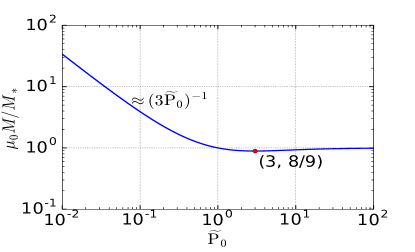
Figure 1: The relation between the normalized peak pressure $\widetilde{P}_{0}$ and the compactness of the horizonless object $\mu_{0}$, given by eq. (15). When $\mu_{0}M/M_{*}\geq 1$ or $\mu_{0}M/M_{*}=8/9$, the peak pressure is unique for each $\mu_{0}M/M_{*}$; when $8/9<\mu_{0}M/M_{*}<1$, each $\mu_{0}M/M_{*}$ corresponds to two different peak pressures (the solution corresponding to the larger pressure is unstable); when $\mu_{0}M/M_{*}<8/9$, the TOV equation with a relativistic EoS $P=\rho/3$ has no solution because, to support gravity, a static configuration requires a local sound speed greater than $c$.

Figure 2: The normalized mass and pressure profiles for $M_{*}/M=10^{-8}$ and $\mu_{0}=10^{-8}$ (solid), $10^{-7}$ (dashed), $10^{-6}$ (dotted).

Shown in Fig. (2) are the mass and pressure profiles for $M_{*}/M=10^{-8}$ and $\mu_{0}=10^{-8},10^{-7},10^{-6}$. The energy density at the bottom of the stellar debris is (in CGS units)

$$\rho(r=r_{0})\approx\frac{M_{*}c^{2}}{4\pi r_{\rm S}^{3}\mu_{0}},$$ (16)

corresponding to a radiation temperature of $T(r=r_{0})\approx 2.9\times 10^{8}(M_{*}/M_{\rm\odot})^{1/4}M_{8}^{-3/4}\mu_{0,-7}^{-1/4}\rm\ K$ (or 25 keV). At this temperature, a small fraction of the radiation could be converted to electron-positron pairs at the bottom of the stellar debris.

Note that it is physically impossible for a horizonless object with compactness $\mu_{0}$ to support a layer of stellar debris of mass $M_{*}>9\mu_{0}M/8$ with a relativistic EoS $P=\rho/3$. For example, in the gravastar model, $r_{0}-r_{\rm S}$ is on the order of Planck length $\sim 10^{-33}\rm\ cm$, so the stellar debris has to switch to the EoS of exotic matter quickly enough to avoid the formation of an event horizon. To avoid going into details of the state transition from baryonic to exotic matter, we consider in this paper only models with $\mu_{0}\gg M_{*}/M$.

3.2 Emission from the photosphere

In this subsection, we go back to CGS units and discuss the emission from the stellar debris on the hard surface of the CMO as viewed by an observer at infinity. We consider the situation where $\mu_{0}\gg M_{*}/M$ (but $\mu_{0}$ is not necessarily much less than 1). The baryonic gas and radiation do not affect the spacetime outside the hard surface, which is given by the Schwarzschild metric for a slowly or non-rotating CMO. We define the function $\mu(r)$ as

$$\mu(r)\equiv-g_{\rm tt}(r)=1-\frac{r_{\rm S}}{r},$$ (17)

where $r_{\rm S}\equiv 2GM/c^{2}$. When $M_{*}\sim 1M_{\rm\odot}$ of baryonic gas falls onto the CMO in nearly the radial direction, the gas collides with the surface at a locally measured Lorentz factor $\mu_{0}^{-1/2}$. The high-density gas downstream of the shock is dominated by radiation pressure, which is given by

$$P_{\rm sh}=\frac{\mu_{0}^{-1/2}-1}{3}\rho_{\rm 0,sh}c^{2},$$ (18)

where $\rho_{\rm 0,sh}$ is the local baryonic mass density right after the shock. Then the stellar debris settles down adiabatically into quasi-hydrostatic equilibrium. When the spacetime outside the CMO hard surface is not affected by the existence of the baryonic gas, the $4\pi r^{3}P$ term in the TOV equation can be ignored. The pressure is dominated by radiation, i.e. $P=P_{\rm rad}+P_{\rm g}\approx P_{\rm rad}$. We denote the local baryonic mass density as $\rho_{0}$, so the total energy density is $\rho=\rho_{0}c^{2}+3P_{\rm g}/2+3P_{\rm rad}\approx\rho_{0}c^{2}+3P$. The TOV equation can then be simplified to

$$\frac{{\mathrm{d}}P}{{\mathrm{d}}r}=-\mu(r)^{-1}\frac{GM\rho_{0}}{r^{2}}\left(1+\frac{4P}{\rho_{0}c^{2}}\right).$$ (19)

If the internal energy per baryon is roughly conserved, we have $P/\rho_{0}\simeq P_{\rm sh}/\rho_{\rm 0,sh}$ and the pressure scale height of the stellar debris at $r=r_{0}$ is

$$H=\mu_{0}\frac{2r_{0}^{2}}{r_{\rm S}}\frac{P_{\rm sh}/(\rho_{\rm 0,sh}c^{2})}{1+4P_{\rm sh}/(\rho_{\rm 0,sh}c^{2})}\simeq\mu_{0}\frac{2r_{0}^{2}}{r_{\rm S}}\frac{1-\sqrt{\mu_{0}}}{4-\sqrt{\mu_{0}}}.$$ (20)

Note that $H$ denotes the scale height in Schwarzschild coordinates; the physical (locally measured) scale height is $H\mu_{0}^{-1/2}$. In the limit $r_{0}\rightarrow r_{\rm S}$ ($\mu_{0}\ll 1$), we get $H\simeq(r_{0}-r_{\rm S})/2$, and in the limit $r_{0}\gg r_{\rm S}$ ($\mu_{0}\approx 1$), we get $H\simeq r_{0}/3$. In reality, part of the internal energy is used to do work against “gravity” (when $\mu_{0}\gtrsim 10^{-6}$, we have $H\mu_{0}^{-1/2}\gtrsim$ solar radius), so the scale height will be smaller (but this has little effect on the analysis since we already have $H<r_{0}-r_{\rm S}$). In addition, part of the internal energy could be used to drive a wind, which might carry a fraction of the total mass $M_{*}$ away at the local escape velocity, so the scale height will be even smaller. We note that the fractional wind mass loss is small ($\ll 1$) because the extra energy taken away by the wind makes the rest of the gas even more bound. We conclude that the pressure or density scale height is roughly a factor of a few smaller than $r_{0}-r_{\rm S}$.

If the total mass of the stellar debris is $M_{*}=\xi M_{\rm\odot}$ ($\xi\lesssim 1$), the Thomson depth of the whole layer is

$$\tau_{0}\simeq\frac{\kappa_{\rm T}M_{*}}{4\pi r_{0}^{2}}\simeq 6.0\times 10^{4}\xi\eta^{-2}M_{8}^{-2},$$ (21)

where we have used the Thomson opacity for solar metallicity, $\kappa_{\rm T}=0.34\rm\ cm^{2}\ g^{-1}$. The photospheric radius $r_{\rm ph}$ (or $\mu_{\rm ph}\equiv\mu(r_{\rm ph})$) where the Thomson scattering optical depth is order unity is larger than $r_{0}+H$ (due to the large total optical depth). For an observer at infinity, the diffusion time across the entire layer of stellar debris is roughly given by

$$\begin{split}t_{\rm dif,\infty}&\simeq\tau_{0}\int_{r_{0}}^{r_{\rm ph}}\frac{{\mathrm{d}}r}{c}\mu^{-1}\simeq\frac{\tau_{0}\eta r_{\rm S}}{c}.\end{split}$$ (22)

During a time $t_{\rm dif,\infty}$, an amount of radiation energy (viewed at infinity) $(1-\mu_{0}^{1/2})M_{*}c^{2}$ diffuses outwards, which gives a diffusive luminosity

$$L_{\rm dif,\infty}\simeq\frac{(1-\mu_{0}^{1/2})M_{*}c^{2}}{t_{\rm dif,\infty}}\simeq(1-\mu_{0}^{1/2})\eta^{-1}L_{\rm Edd},$$ (23)

where the Eddington luminosity is $L_{\rm Edd}\equiv 4\pi cGM/\kappa_{\rm T}=1.5\times 10^{46}M_{8}\rm\ erg\ s^{-1}$. From eq. (23), we find that $L_{\rm dif,\infty}\simeq L_{\rm Edd}$ when either $\mu_{0}\ll 1$ or $\mu_{0}\approx 1$. Including gravitational redshift, the diffusive flux in the local rest frame at $\mu(r)$ is $\simeq L_{\rm Edd}\mu^{-1}$, which means that the radiation force on the baryon-photon mixture balances gravity.

Photons emitted at the photosphere at radius $r_{\rm ph}$, or $\mu_{\rm ph}\equiv\mu(r_{\rm ph})$, may not escape to infinity. The maximum polar angle $\theta_{\rm m}$ up to which photons emitted at $r_{\rm ph}$ can escape to infinity is given by

$$\begin{split}\theta_{\rm m}=&\pi/2\mbox{, if $r_{\rm ph}>1.5r_{\rm S}$,}\\ \theta_{\rm m}=&\mathrm{sin}^{-1}\frac{3\sqrt{3}\mu_{\rm ph}^{1/2}}{2r_{\rm ph}/r_{\rm S}}\mbox{, if $r_{\rm ph}\leq 1.5r_{\rm S}$.}\end{split}$$ (24)

The luminosity seen by an observer at infinity is the fraction of $L_{\rm dif,\infty}$ that escapes, i.e.

$$L_{\rm\infty}=L_{\rm dif,\infty}\frac{\int_{0}^{\rm\theta_{\rm m}}I(\theta)\cos\theta\sin\theta{\mathrm{d}}\theta}{\int_{0}^{\pi/2}I(\theta)\cos\theta\sin\theta{\mathrm{d}}\theta},$$ (25)

where $L_{\rm dif,\infty}=8\pi^{2}r_{\rm ph}^{2}\int_{0}^{\pi/2}I(\theta)\cos\theta\sin\theta{\mathrm{d}}\theta\simeq L_{\rm Edd}$. The intensity is nearly angle independent $I(\theta)\simeq I$, so we have

$$L_{\rm\infty}\simeq L_{\rm Edd}\sin^{2}\theta_{\rm m}.$$ (26)

For any given angle, the spectrum is nearly a blackbody $I_{\nu}\simeq B_{\nu}(T_{\rm ph})$ (e.g. Broderick & Narayan, 2006), so we have $I\simeq\sigma_{\rm SB}T_{\rm ph}^{4}/\pi$, where $\sigma_{\rm SB}$ is the Stefan-Boltzmann constant and $T_{\rm ph}$ is the local radiation temperature at the photosphere. Therefore, the radiation temperature at infinity is

$$\begin{split}T_{\rm\infty}&=T_{\rm ph}\mu_{\rm ph}^{1/2}=\left(\frac{L_{\rm Edd}}{4\pi r_{\rm ph}^{2}\sigma_{\rm SB}}\right)^{1/4}\mu_{\rm ph}^{1/4}\\ &\simeq 3.9\times 10^{5}\left(\frac{r_{\rm S}}{r_{\rm ph}}\right)^{1/2}M_{8}^{-1/4}\mu_{\rm ph}^{1/4}\rm\ K.\end{split}$$ (27)

The duration of the emission from the stellar debris is given by energy conservation

$$\Delta t_{\rm\infty}=(1-\mu_{0}^{1/2})\frac{\xi M_{\rm\odot}c^{2}}{L_{\rm\infty}}\simeq 1.2\times 10^{8}\frac{\xi(1-\mu_{0}^{1/2})}{M_{8}\sin^{2}\theta_{\rm m}}\rm\ s.$$ (28)

Note that in the limit $\mu_{\rm ph}\ll 1$ (and $\eta\approx 1$), the duration of the transient emission in eq. (28) is longer than the diffusion time given by eq. (22) by a factor $\mu_{\rm ph}^{-1}$. This is because photons emitted at the photosphere tend to be lensed back $\mu_{\rm ph}^{-1}$ times before escaping (a photon can escape only when $\theta\leq\theta_{\rm m}$).

In the upper panel of Fig. (3), we show in red lines the g-band ($\simeq 4800\rm\ \AA$) flux density as a function of the photospheric radius $r_{\rm ph}$, for three different CMO masses, $M=10^{7.5}$, $10^{8.5}$ and $10^{9.5}\rm\ M_{\rm\odot}$, at redshift $z=0.5$. The limiting flux for the Pan-STARRS1 3$\pi$ survey (PS1, thick green line) and the Large Synoptic Survey Telescope 3$\pi$ survey (LSST, thin green line) are calculated by assuming the source to be at least 1.5 mag brighter than the 5$\sigma$ flux limit for a single exposure ($M_{\rm AB}=22.0$ and 23.4 mag for PS1 and LSST respectively, see section 4 for details of the two telescopes). We also show in red lines the blackbody temperature for an observer at infinity as a function of $r_{\rm ph}$.

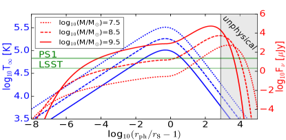
Figure 3: For an observer at infinity, the emission from the layer of stellar debris on the hard surface has a blackbody spectrum with luminosity given by eq. (26) and temperature given by eq. (27). The duration of the emission is given by eq. (28). In the Upper Panel, we show in red lines the g-band flux density as a function of the photospheric radius $r_{\rm ph}$, for three different CMO masses, $M=10^{7.5}\rm\ M_{\rm\odot}$ (dotted), $10^{8.5}\rm\ M_{\rm\odot}$ (dashed) and $10^{9.5}\rm\ M_{\rm\odot}$ (solid), at redshift $z=0.5$. The limiting flux for Pan-STARRS1 3$\pi$ survey (PS1, thick green line) and LSST (thin green line) are calculated by assuming the source to be 1.5 mag brighter than the 5$\sigma$ sensitivity for a single exposure. For CMOs heavier than $10^{7.5}M_{\rm\odot}$, the photospheric radius must be smaller than $7.6\times 10^{2}r_{\rm S}$ (otherwise the entire baryonic layer is Thomson thin), so the grey shaded region is unphysical. We also show in blue lines the radiation temperature for an observer at infinity as a function of $r_{\rm ph}$. In the Lower Panel, we show the duration of the emission $\Delta t_{\infty}$ as a function of $r_{\rm ph}$ when the total mass of the stellar debris is $M_{*}=0.5M_{\rm\odot}$ ($\xi=0.5$). The grey/blue regions denote the timescales over which PS1/LSST are complete, with the upper bound given by the survey lifespan and the lower bound given by the cadence (see section 4 for details of the two telescopes). We only show the parameter space $r_{\rm ph}/r_{\rm S}-1\lesssim 1$, because in this regime $\Delta t_{\infty}$ is only a function of $r_{\rm ph}$ but not $r_{0}$ (since $\mu_{0}\approx 1$). As we show in section 4, the parameter space $r_{\rm ph}/r_{\rm S}-1\gtrsim 1$ has already been ruled out by PS1.

When $r_{\rm ph}/r_{\rm S}-1\ll 1$, we have $\mu_{\rm ph}\approx r_{\rm ph}/r_{\rm S}-1$, $L_{\rm\infty}\propto\mu_{\rm ph}$ and $T_{\infty}\propto\mu_{\rm ph}^{1/4}$. For $10^{-5}\lesssim r_{\rm ph}/r_{\rm S}-1\ll 1$, the g-band frequency is in the Rayleigh-Jeans regime, so the flux density decreases slowly as $F_{\nu}\propto\mu_{\rm ph}^{1/4}$. For $\mu_{\rm ph}\lesssim 10^{-5}$, the g-band frequency slowly shifts into the Wien tail, so the flux density drops faster. On the other hand, for $r_{\rm ph}/r_{\rm S}-1\gg 1$, the temperature decreases rapidly as $T_{\infty}\propto r_{\rm ph}^{-1/2}$, but the luminosity stays constant at $L_{\rm Edd}$. Therefore, the flux density first increases as $F_{\rm\nu}\propto r_{\rm ph}^{3/2}$ in the Rayleigh-Jeans regime and then decreases exponentially in the Wien regime.

Note that the optical depth for Thomson scattering at the photosphere is of order unity, so this gives an upper limit for the photospheric radius,

$$4\pi r_{\rm ph}^{2}<\kappa_{\rm T}M_{*},$$ (29)

which means

$$\frac{r_{\rm ph}}{r_{\rm S}}<7.6\times 10^{2}\xi^{1/2}M_{7.5}^{-1}.$$ (30)

For $\xi\lesssim 1$ and the CMO mass range $M>10^{7.5}M_{\rm\odot}$ considered in this paper, the photospheric radius of the stellar debris layer must be smaller than $7.6\times 10^{2}r_{\rm S}$, so the grey shaded region in the upper panel of Fig. (3) is unphysical. For CMOs with mass $M<10^{7.5}M_{\rm\odot}$, the emission from the stellar debris may peak in the non-observable far UV (if $r_{\rm ph}/r_{\rm S}-1\lesssim 1$), so one does not obtain strong constraints on the radius of the hard surface. In addition, stars get tidally disrupted before reaching close to the Schwarzschild radius, so the actual accretion rate is uncertain due to the complexities of accretion disk physics.

In the lower panel of Fig. (3), we show the emission duration $\Delta t_{\infty}$ as a function of $r_{\rm ph}$ for the same stellar mass $M_{*}=0.5M_{\rm\odot}$ ($\xi=0.5$) and three CMO masses. From eq. (28), we see that $\Delta t_{\infty}$ is a function of both the hard surface radius $r_{0}$ (or $\mu_{0}$) and the photospheric radius $r_{\rm ph}$. As we show in section 4, observations from PS1 have already ruled out the parameter space $r_{\rm ph}/r_{\rm S}-1\gtrsim 1$, so here we only show the parameter space $r_{\rm ph}/r_{\rm S}-1\lesssim 1$, where $\Delta t_{\infty}$ is only a simple function of $r_{\rm ph}$ (because $\mu_{0}\ll 1$). We note that $\Delta t_{\rm\infty}\propto\mu_{\rm ph}^{-1}$ in the limit of $\mu_{\rm ph}\ll 1$. Therefore, if the CMO is compact enough, the duration may become longer than the average time interval between two stellar disruption events and persistent emission from CMOs could be searched for.

To link the observational constraints on the photospheric radius $r_{\rm ph}$ to the physical limits on the hard surface radius $r_{0}$, we need to calculate the baryonic density profile of the stellar debris layer. The detailed density profile of the stellar debris could in principle be obtained by considering the radiation transfer and gravity with appropriate EoS and boundary conditions (e.g. Paczynski & Anderson, 1986; Wielgus et al., 2016). For the purpose of this paper, we only need to consider the baryonic density profile in the optically thick region in the limit $\mu_{\rm ph}\ll 1$. The system reaches hydrostatic equilibrium roughly on the light-crossing timescale $\sim r_{\rm S}/c$ (or a logarithmic factor larger), which is much smaller than the diffusion time, so the evolution of the stellar debris can be considered as adiabatic and we have $P(\mu)\propto[\rho_{0}(\mu)]^{4/3}$ (it is more convenient to use $\mu$ instead of the radial coordinate $r$). From section 3.1, we know $P(\mu)\propto\mu^{-2}$, so the baryonic density profile is $\rho_{0}(\mu)\propto\mu^{-3/2}$. The normalization is given by the total mass $M_{*}=\int_{r_{0}}^{r_{1}}4\pi r^{2}\rho_{0}(r)\mu^{-1/2}{\mathrm{d}}r$, so we have

$$\rho_{0}(\mu)=\frac{M_{*}}{4\pi r_{\rm S}^{3}\mu_{0}^{1/2}}\left(\frac{\mu}{\mu_{0}}\right)^{-3/2}.$$ (31)

From the rest mass density and temperature (eq. 16), we get the ratio between the (non-relativistic) electron degeneracy pressure and gas pressure $P_{\rm deg}/P_{\rm g}\simeq 2\times 10^{-7}(M_{*}/M_{\rm\odot})^{5/12}M_{8}^{-5/4}\mu_{0,-7}^{-1/12}(\mu/\mu_{0})^{-1/2}$. The ratio between gas pressure and radiation pressure is $P_{\rm g}/P_{\rm rad}\simeq 10^{-8}(M_{*}/M_{\rm\odot})^{1/4}M_{8}^{-3/4}\mu_{0,-7}^{1/4}$. Therefore, the pressure is completely dominated by radiation. The Thomson optical depth above a certain radius $\mu(r)$ is

$$\tau(\mu)=\frac{\kappa_{\rm T}}{4\pi r_{\rm S}^{2}}\int_{r}^{r_{1}}4\pi r^{2}\rho_{0}(r)\mu^{-1/2}{\mathrm{d}}r=\frac{\kappa_{\rm T}M_{*}}{4\pi r_{\rm S}^{2}}\frac{\mu_{0}}{\mu}.$$ (32)

Therefore, the relation between the photospheric radius $r_{\rm ph}$ and the hard surface radius $r_{0}$, in the limit $\mu_{\rm ph}\ll 1$, is

$$\mu_{\rm ph}\simeq\mu_{0}\frac{\kappa_{\rm T}M_{*}}{4\pi r_{\rm S}^{2}}.$$ (33)

For a given CMO mass $M$, as long as $\mu_{0}>4\pi r_{\rm S}^{2}/(\kappa_{\rm T}M_{*})$, the photospheric radius is at $r_{\rm ph}/r_{\rm S}-1\gtrsim 1$. As shown in Fig. (3), the g-band flux density increases roughly as $r_{\rm ph}^{3/2}$ in this regime. Instead of solving for the detailed baryonic density profile when $r_{\rm ph}/r_{\rm S}-1\gtrsim 1$, we take a conservative limit

$$\frac{r_{\rm ph}}{r_{\rm S}}-1=\mbox{min}\left[\mu_{0}\tau_{0},\ \mbox{max}\left(0.3,~{}\frac{r_{0}}{r_{\rm S}}-1\right)\right],$$ (34)

where $\tau_{0}=\kappa_{\rm T}M_{*}/(4\pi r_{0}^{2})\simeq 6.0\times 10^{4}\xi\eta^{-2}M_{8}^{-2}$. Eq. (34) and $\mu_{\rm ph}=1-r_{\rm S}/r_{\rm ph}$, as well as eqs. (26), (27) and (28), will be used in section 4 to calculate a lower limit on the observed the flux density for a CMO of given mass at a given redshift. One more point to note is that, when considering $\eta\gg 1$, we discard the (very few) high mass CMOs that give $\tau_{0}\leq 10$, to make sure that the radiation field is well thermalized.

4 Observations

In this section, we assume the total baryonic mass of the stellar debris layer to be $M_{*}=\xi M_{\rm\odot}=0.5M_{\rm\odot}$. For a given CMO of mass $M$ and redshift $z$, the flux density at frequency $\nu$ on the Earth is

$$F_{\nu}=\frac{15}{\pi^{4}}\frac{L_{\rm\infty}}{4\pi D_{\rm L}^{2}}\frac{x^{4}/\nu}{\mathrm{e}^{x}-1},$$ (35)

where $x=h\nu(1+z)/(kT_{\rm\infty})$, $h$ is the Planck constant, $k$ is the Boltzmann constant, and $D_{\rm L}(z)$ is the luminosity distance. For a survey with limiting flux $F_{\nu}^{\rm lim}$, we can calculate the limiting redshift $z^{\rm lim}$ by solving $F_{\nu}(z)=F_{\nu}^{\rm lim}$. If we know the mass function of CMOs, $\Psi(M,z)$ (comoving number density of CMOs of different masses at a given redshift), we can calculate the expected detectable event rate within a solid angle $\Delta\Omega$ on the sky

$$\dot{N}_{\rm det}=\int_{M_{\rm min}}^{M_{\rm max}}\mathrm{d}M\dot{N}(M)\int_{0}^{z_{\rm lim}}\mathrm{d}z\Psi(M,z)\frac{\mathrm{d}V}{\mathrm{d}\Omega\mathrm{d}z}\Delta\Omega,$$ (36)

where $\dot{N}(M)$ is the stellar disruption rate for a given CMO of a certain mass, $M_{\rm min}=10^{7.5}M_{\rm\odot}$ is the minimum mass we consider, $M_{\rm max}=10^{9}M_{\rm\odot}$ is the maximum mass we consider, and $\mathrm{d}V/(\mathrm{d}\Omega\mathrm{d}z)$ is the comoving volume per unit redshift per steradian.

We use the CMO mass function $\Psi(M,z)$ by Shankar et al. (2009), who integrate from the low-redshift CMO mass function backwards over cosmic time with the growth/accretion rate empirically derived from AGN luminosity function and a prescribed radiation efficiency. We ignore the (small) contribution from CMOs at $z>5$, due to large uncertainties on the mass function at high redshift. We have also tried the mass function given by Merloni & Heinz (2008), who use the same method as Shankar et al. (2009), and the differences are negligible. The CMO mass function can also be derived by linking their growth to the properties of host dark matter haloes. For instance, in Hopkins et al. (2008), the CMO masses are assumed to be proportional to the host spheroidal mass, as the host dark matter haloes grow through major mergers. Various CMO mass function models are reviewed by Kelly & Merloni (2012). At redshift $z<5$, they agree to within a factor $\lesssim 3$ in the range $10^{7.5}$-$10^{9}M_{\rm\odot}$ and they all have rapid drop-offs above $\sim 10^{9}M_{\rm\odot}$.

If we know $\Psi(M,z)$ well enough, the question comes down to the stellar disruption rate $\dot{N}$ per CMO, which is defined as the sum of the rates of the following three possibilities: (1) the star passes within the tidal disruption radius $r_{\rm T}$; (2) the specific angular momentum of the orbit is less than $2r_{\rm S}c$ (corresponding to a Newtonian parabolic orbit with pericenter distance of $r_{\rm p}=4r_{\rm S}$); (3) the star directly collides with the surface at radius $r_{0}$. These rates depend on the stellar phase-space distribution and the galactic gravitational potential (and other factors mentioned in section 1). If various CMO-host-galaxy correlations (e.g. Kormendy & Ho, 2013) are used, such as $M$-$\sigma$ (velocity dispersion) and $M$-$L_{\rm bulge}$ (bulge luminosity), we can quantify the stellar disruption rate $\dot{N}$ purely as a function of the CMO mass.

The disruption rate has been extensively calculated for different samples of elliptical galaxies (e.g. Magorrian & Tremaine, 1999; Wang & Merritt, 2004; Stone & Metzger, 2016). We note that previous authors chose the critical pericenter distance to be $r_{\rm p}=r_{\rm T}$, so when $r_{\rm T}<\mathrm{max}(r_{0},4r_{\rm S})$, the size of the “loss cone” and hence the disruption rate were underestimated. However, for a given CMO mass and stellar phase-space distribution, $\dot{N}$ depends weakly on the critical pericenter distance $r_{\rm p}$ (roughly as $r_{\rm p}^{1/4}$), so the error on the derived disruption rate is small.

Typically, the disruption rate per CMO as a function of the CMO mass can be described as a power-law,

$$\dot{N}=\dot{N}_{0}M_{6.5}^{-\delta},$$ (37)

but the parameters $\dot{N}_{0}$ and $\delta$ depend strongly on the galaxy sample. There is a bimodal distribution of central surface brightness profiles in early-type galaxies (e.g. Lauer et al., 2007). The disruption rates in cusp galaxies (brightness power-law index $\gamma>0.2$) are a factor of $\sim 10$ higher than in core galaxies ($\gamma<0.2$) with the same CMO mass. The power-law indexes $\delta$ derived from only cusp or core galaxies in Lauer et al. (2007) are $\delta\simeq 0.25$, but the power-law is significantly steeper, $\delta\sim 0.4$-0.5, when the entire sample is considered (Stone & Metzger, 2016). This is because core galaxies (with lower $\dot{N}$) generally host more massive CMOs than cusp galaxies (with larger $\dot{N}$). Other factors, e.g. non-spherical and time-dependent galactic potential, binary CMOs, massive perturbers, add further uncertainties on the disruption rates. It is currently not possible to calculate the disruption rates as a function of CMO mass (for recent discussions, see Vasiliev & Merritt, 2013; Merritt, 2013; Kochanek, 2016).

On the observational side, several dozen TDE flares have recently been discovered in surveys from optical to X-ray wavelengths, and the TDE rate is found to be $\sim 10^{-5}\rm\ galaxy^{-1}yr^{-1}$ (Donley et al., 2002; Gezari et al., 2008; Wang et al., 2012; van Velzen & Farrar, 2014; Holoien et al., 2016). As pointed out by Stone & Metzger (2016), there is a factor of $\sim 10$ disagreement between the observational and theoretical TDE rates, which could be due to either observational incompleteness (e.g. dust extinction or incomplete wavelength coverage), over-estimate of the brightness of most TDEs (e.g. Guillochon & Ramirez-Ruiz, 2015), or missing physics in TDE rate calculations (e.g. time-dependent gravitational potential). French et al. (2016) show that optical-UV TDEs favor post starburst galaxies with CMO mass in the range $10^{5.5}$-$10^{7.5}\rm\ M_{\rm\odot}$, and hence normal star-forming and early-type galaxies may have a much lower TDE rate. This makes the tension between observational and theoretical TDE rates even stronger. Larger samples in the future will help to illuminate this puzzle.

In the following, we take a conservative estimate for the observed TDE rate, $\dot{N}_{0}=1\times 10^{-5}\rm\ M_{\rm\odot}\ yr^{-1}$, and leave the power-law index $\delta\in[0.2,0.5]$ as a free parameter. With the detectable event rate $\dot{N}_{\rm det}$ from eq. (36), we need the effective monitoring time $t_{\rm eff}$ to calculate the expected number of detections for a given survey. If the transient emission has duration $(1+z)\Delta t_{\rm\infty}$ (eq. 28) and the survey has total lifespan $t_{\rm tot}$ and cadence $t_{\rm cad}$, the effective monitoring time is

$$t_{\rm eff}(M,z)=\frac{t_{\rm tot}}{t_{\rm cad}}\mbox{min}[(1+z)\Delta t_{\infty},t_{\rm cad}]-(1+z)\Delta t_{\infty}.$$ (38)

Note that in eq. (38) we have assumed: (1) the time interval between any two consecutive exposures is always $t_{\rm cad}$; (2) detection(s) of the transient emission must be preceded and followed by non-detections, i.e. only the cases with “off-on-off” are considered as positive signals but cases with “on-off” or “off-on” are discarded in order to be conservative. Therefore, for a certain hard surface radius $\eta=r_{0}/r_{\rm S}$, the expected number of detections is

$$\begin{split}N_{\rm det}=&\ \int_{M_{\rm min}}^{M_{\rm max}}\mathrm{d}M\dot{N}(M)\\ &\times\int_{0}^{z_{\rm lim}(M,\eta)}\mathrm{d}z\Psi(M,z)t_{\rm eff}(M,z)\frac{\mathrm{d}V}{\mathrm{d}\Omega\mathrm{d}z}\Delta\Omega.\end{split}$$ (39)

In Fig. (4), we show the expected number of detections for two different surveys as a function of the hard surface radius $r_{0}$. Solid lines are for g-band observations by the Pan-STARRS1 3$\pi$ survey (PS1, Kaiser et al., 2010; Inserra et al., 2013; Chambers et al., 2016), and dashed lines are for future g-band observations by the Large Synoptic Survey Telescope 3$\pi$ survey (LSST, Ivezic et al., 2008). Different line colors represent different disruption rate power-law slopes ($\delta$ in eq. 37). Both surveys cover 3/4 of the sky, but since low Galactic-latitude regions have significant dust extinction, we use sky area $\Delta\Omega=2\pi$. For a single exposure, PS1 and LSST have g-band 5-$\sigma$ flux limit of 22.0 and 23.4 in AB magnitude, and we only consider sources 1.5 mag brighter than the 5-$\sigma$ limits for the calculation of the number of detectable events.

PS1 3$\pi$ survey has a cadence of $t_{\rm cad}\simeq$ 3 months and total operation time of $t_{\rm tot}\simeq$ 3.5 years (so far). LSST 3$\pi$ survey will have a cadence of $t_{\rm cad}\simeq$ 3 days and total lifespan of $t_{\rm tot}\simeq$ 10 years. The transient searching data products (from image subtraction) of PS1 have been released to the public (Huber et al., 2015; Flewelling et al., 2016). If CMOs have a hard surface, stellar disruption events produce transients that are distinct from traditionally known ones (e.g. supernovae, ANG, variable stars, etc.), because they have thermal spectra with year-long smooth lightcurves. Currently, no such transients have been reported.

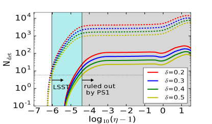
Figure 4: Expected number of stellar disruption events detectable by Pan-STARRS1 (PS1, solid lines) and LSST (dashed lines) as a function of the hard surface radius $r_{0}=\eta r_{\rm S}$. (Note that this plot considers $r_{0}$ along the abscissa, whereas Fig. 3 considers the photospheric radius $r_{\rm ph}$.) Different colors represent different disruption rate power-law slopes ($\delta$ in eq. 37 varying from 0.2 to 0.5). Non-detection throughout the survey lifespan rules out the region above $N_{\rm det}=5.81$ (thin horizontal dotted line) at 99.7% confidence level. For the conservative disruption rate power-law index $\delta=0.5$, observations by PS1 have ruled out the grey shaded region $\eta-1>10^{-4.4}$. Future observations by LSST will be able to improve the limit to $\sim 10^{-6}$. The sharp drop at the smallest $\eta$ is caused by the duration of transient emission approaching the survey lifespan. The flat part in the middle is when $r_{\rm ph}/r_{\rm S}-1$ approaches order of unity and we simply take $r_{\rm ph}/r_{\rm S}-1=0.3$ as a conservative limit in eq. (34) (larger $r_{\rm ph}$ gives higher g-band flux density). The rising part at $\eta-1\gtrsim 1$ is caused by the radiation temperature decreasing with $r_{\rm ph}$ when $r_{\rm ph}/r_{\rm S}-1\gtrsim 1$ (see the upper pannel of Fig. 3). The drop when $\eta-1$ approaches 30 is caused by the duration of the transient emission being shorter than the survey cadence. We only consider the parameter space $1<\eta<30$ in this paper (the upper limit arises from the fact that TDEs from $\gtrsim 10^{6}M_{\rm\odot}$ CMOs have been observed).

The actual number of detections follows a Poisson distribution with expectation value $N_{\rm det}$, so non-detection rules out the region above the horizontal thin dotted line with $N_{\rm det}=5.81$ in Fig. 4 at confidence level $1-\mathrm{exp}(-5.81)=99.7\%$. For instance, for the conservative case $\delta=0.5$, any hard surface above $r_{0}/r_{\rm S}-1=10^{-4.4}$ can be ruled out by PS1. The lower limit depends on the slope of the stellar disruption rate and ranges from $10^{-4.8}$ to $10^{-4.4}$ when $\delta$ goes from 0.2 to 0.5. With the same argument presented in this paper, future observations by LSST may be able to rule out $r_{0}/r_{\rm S}-1\gtrsim 10^{-6}$ (limited by the duration of the transient emission). We also note that only the information from g-band is used, and if we combine g-band limits with other bands (urizy), the constraints are slightly stronger.

5 Discussion

The main conclusions of this work can be found in the abstract and Figs. (3) and (4). We discuss possible issues in the analysis above.

(1) We have assumed that all CMOs have a universal $\eta=r_{0}/r_{\rm S}$ (the ratio of CMO hard surface radius $r_{0}$ to the event horizon radius $r_{\rm S}$). However, the existing data does not rule out the possibility that a small fraction of CMO might have $\eta-1>10^{-4.4}$. In the future LSST era, with a much more accurate determination of the rate of stellar disruptions by CMOs, one should be able to place a much stronger limit on $\eta-1$ without making the assumption that all CMOs have the same $\eta$.

(2) We have ignored the spin of CMOs, which will modify the shape of the hard surface and spacetime above the surface (and hence the emergent radiation from the stellar debris). Note that the scale height of the layer of stellar debris is a factor of a few smaller than $r_{0}-r_{\rm S}$ in the non-spinning case. And as long as the spin is relatively slow (spin parameter $a/M\lesssim 0.2$), most of the baryonic mass is within the light cylinder and the structure of the stellar debris layer is not strongly affected by rotation. The emission from the photosphere is still determined by the fraction of the diffusive flux escaping to infinity, so observations can rule out a similar range of $\eta$ as shown in Fig. (4) and the conclusion will be similar for CMOs with $a/M\lesssim 0.2$.

(3) The situation close to the photosphere in the strong-gravity regime is complicated: (i) the radiation field is highly anisotropic; (ii) baryons and radiation cannot be treated as a single fluid; (iii) the system is not adiabatic due to energy flowing in from below and out from above; (iv) there might be large-scale convective motion or wind. One caveat of this paper is that the lightcurve of the transient emission is likely not flat. The hydrodynamics of the collision between the star and the hard surface can affect the initial lightcurve on a timescale of a few times $r_{\rm S}/c$ or possibly as large as $\mu_{\rm ph}^{-1}r_{\rm S}/c$ (when $\mu_{\rm ph}\ll 1$). Then, since the flux of photons escaping to infinity is smaller than the diffusive flux arriving at the photosphere from deeper layers, the radiation pressure at the photosphere rises with time causing a larger escaping flux and also pushing the photosphere to slightly larger radii. On a timescale longer than the photon diffusion time through the entire layer (see eq. 22), the photosphere slowly shrinks and the escaping flux decreases with time until the radiation energy content is depleted. Solving the full radiation-hydrodynamical structure of the stellar debris layer from optically thick to thin regions is left for future work. We discuss in Appendix A the validity and limitations of the TOV equation for describing the structure of the stellar debris layer.

(4) We were unable to provide a strong constraint on $\eta$ for CMOs of mass $<10^{7.5}M_{\odot}$, due to the following two reasons: (i) the emission from the layer of stellar debris on the possible hard surface may peak in the non-observable far UV (if $r_{\rm ph}/r_{\rm S}-1\sim 1$); (ii) main-sequence stars are tidally disrupted before reaching close to $r_{\rm S}$. The radiation produced (e.g. by shocks and the accretion disk) before the gas falls onto the CMO makes it very hard for observations to constrain the emission we have calculated in this work. The actual accretion rate onto the CMO is also uncertain due to the complexities of accretion disk physics.

(5) We have assumed that baryons and radiation associated with the stellar debris are incorporated into the CMO’s pre-existing exotic material (the material that forms the hard surface with which the star collides) on a timescale $t_{\rm in}$ much longer than the duration of the transient radiation from stellar disruption, $\Delta t_{\infty}$, given by eq. (28). If $t_{\rm in}$ were to be less than $\sim r_{\rm S}/c$, the layer of stellar debris is converted to the exotic matter before baryons can reach hydrostatic equilibrium, and in this case very little radiation will escape to infinity. If $r_{\rm S}/c\ll t_{\rm in}<\Delta t_{\infty}$, the debris has sufficient time to reach hydrostatic equilibrium and its stratification is correctly described in section 3.1. However, the transient radiation from this stratified debris does not last for the full time duration $\Delta t_{\infty}$ (calculated in section 3.2), but is terminated earlier ($t_{\rm in}$) when the transformation of the debris to the exotic matter is completed.

(6) CMOs are growing in mass $M$ and size $r_{0}$ due to gas accretion over cosmic time. To avoid the formation of an event horizon, the mass of the baryonic layer on the hard surface must not exceed $9\mu_{0}M/8$ (see Fig. 1). Therefore, the transformation of radiation-baryon mixture to exotic matter must occur on a timescale $t_{\rm in}\lesssim\mu_{0}M/\dot{M}$ ($\dot{M}$ being the accretion rate). This assumption was implicitly made by Broderick et al. when they considered the consequences of accretion onto a possible hard surface in Sgr A* and M87* (e.g. Broderick et al., 2015). Furthermore, they assumed, based on an erroneous reasoning from the short dynamical time ($\sim r_{\rm S}/c$), that the system can be described to be in equilibrium such that the rate of radiation energy escaping to infinity is equal to the rate of mass-energy falling onto the hard surface, i.e. $L_{\infty}\simeq\dot{M}c^{2}$. However, we point out that the dynamical time being short only means that the baryonic layer on the hard surface is in hydrostatic equilibrium, but it does not imply a balance between the rate of in-falling and escaping energy. The luminosity at infinity is equal to the accretion rate when the timescale for radiation to escape from the hard surface is shorter than the timescale over which the accretion rate is roughly constant. For Sgr A*, the accretion rate likely varies on timescales of $t_{\rm acc}<Mc^{2}/L_{\rm Edd}\simeq 3.8\times 10^{8}\rm\ yr$. If the radiation from the accreted gas is released at radius $r$ where $\mu(r)\approx r/r_{\rm S}-1\ll 1$, then only a small fraction $\mu$ of the radiation escapes and the rest follows a highly curved trajectory that brings it back to the hard surface. Therefore, photons bounce on the hard surface $\sim\mu^{-1}$ times before escaping to infinity. Thus, the time it takes for photons to escape from the hard surface is $t_{\rm esc}\sim\mu^{-1}r_{\rm S}/c$. For Sgr A* we have $t_{\rm acc}/t_{\rm esc}\sim 10^{14}\mu(t_{\rm acc}/10^{8}\rm\ yr)$, and hence if $\mu\ll 10^{-14}$ then $L_{\infty}\ll\dot{M}c^{2}$. It follows from this result that for Sgr A* a hard surface at radius $r_{0}/r_{\rm S}-1\ll 10^{-14}$ cannot be ruled out. Moreover, if transformation of ordinary matter to whatever exotic matter makes up the hard surface occurs on a short timescale $t_{\rm in}\lesssim r_{\rm S}/c$, very little radiation will escape from the CMO and the object would be indistinguishable from a BH in its electromagnetic signal. As pointed out by Abramowicz et al. (2002), the approach of Broderick et al., and the work presented here, supports the existence of the event horizon but does not provide a firm proof; these works do, however, severely constrain the location of the hard surface to be extremely close to the Schwarzschild radius, with $r_{0}/r_{\rm S}-1\lesssim 10^{-4}$ for CMOs of $M>10^{7.5}M_{\rm\odot}$ in other galaxies, and $\lesssim 10^{-14}$ for Sgr A*.

6 acknowledgments

We thank Edward Robinson, Emil Mottola and James Guillochon for useful discussions. We also thank the anonymous referee for useful comments. WL was funded by the Named Continuing Fellowship at the University of Texas at Austin. RN was supported in part by NSF grant AST1312651, NASA grant TCAN NNX14AB47G, and the Black Hole Initiative at Harvard University, which is supported by a grant from the John Templeton Foundation.

Appendix A

We show that matter is well coupled to radiation in the optically thick part of the layer, but not when the optical depth drops below $\sim 10$.

Consider an electron (associated with a proton) moving through an isotropic radiation field. The distance it travels before being forced to change direction by Compton scattering can be estimated by

$$d_{\rm sc}\sim\frac{m_{p}c^{2}}{\sigma_{\rm T}\rho},$$ (40)

where $\rho$ is the radiation energy density, given by

$$\rho(\mu)\simeq\frac{M_{*}c^{2}}{4\pi r_{\rm S}^{3}\mu_{0}}\left(\frac{\mu}{\mu_{0}}\right)^{-2}.$$ (41)

Putting eq. (41) into eq. (40), we obtain

$$d_{\rm sc}\sim\frac{\mu r_{\rm S}}{\tau(\mu)}\sim\mu^{1/2}\lambda\ll\lambda,$$ (42)

where $\tau(\mu)=\kappa_{T}M_{*}\mu_{0}/(4\pi r_{\rm S}^{2}\mu)$ is the optical depth above $\mu(r)$ and $\lambda\sim\mu^{1/2}r_{\rm S}/\tau(\mu)$ is the local Thomson mean free path. The radiation temperature at location $\mu(r)$ is $kT(\mu)\simeq 25(M_{*}/M_{\rm\odot})^{1/4}M_{8}^{-3/4}\mu_{0,-7}^{1/4}\mu_{-7}^{-1/2}\rm\ keV$, so the thermal speed of protons is non-relativistic. Therefore, baryons diffuse very slowly and are well coupled to the local radiation field (which dominates the energy density). This coupling breaks down as we approach the photosphere and $\tau(\mu)$ becomes less than about 10. Furthermore, the radiation field and the pressure tensor become highly anisotropic for $\tau\lesssim 10$, and the TOV equation no longer provides a good description of the structure of the layer above this point.

References

- Abbott et al. (2016) Abbott, B. P., Abbott, R., Abbott, T. D., et al. 2016, Physical Review Letters, 116, 221101
- Abramowicz et al. (2002) Abramowicz, M. A., Kluźniak, W., & Lasota, J.-P. 2002, A&A, 396, L31
- Alexander (2005) Alexander, T. 2005, Physics Reports, 419, 65
- Arcavi et al. (2014) Arcavi, I., Gal-Yam, A., Sullivan, M., et al. 2014, ApJ, 793, 38
- Broderick & Narayan (2007) Broderick, A. E., & Narayan, R. 2007, Classical and Quantum Gravity, 24, 659
- Broderick & Narayan (2006) Broderick, A. E., & Narayan, R. 2006, ApJL, 638, L21
- Broderick et al. (2009) Broderick, A. E., Loeb, A., & Narayan, R. 2009, ApJ, 701, 1357
- Broderick et al. (2015) Broderick, A. E., Narayan, R., Kormendy, J., et al. 2015, ApJ, 805, 179
- Buchdahl (1959) Buchdahl, H. A. 1959, Phys. Rev., 116, 1027
- Chambers et al. (2016) Chambers, K. C., Magnier, E. A., Metcalfe, N., et al. 2016, arXiv:1612.05560
- Doeleman et al. (2008) Doeleman, S. S., Weintroub, J., Rogers, A. E. E., et al. 2008, Nature, 455, 78
- Doeleman et al. (2012) Doeleman, S. S., Fish, V. L., Schenck, D. E., et al. 2012, Science, 338, 355
- Donley et al. (2002) Donley, J. L., Brandt, W. N., Eracleous, M., & Boller, T. 2002, AJ, 124, 1308
- Flewelling et al. (2016) Flewelling, H. A., Magnier, E. A., Chambers, K. C., et al. 2016, arXiv:1612.05243
- French et al. (2016) French, K. D., Arcavi, I., & Zabludoff, A. 2016, ApJL, 818, L21
- Gezari et al. (2008) Gezari, S., Basa, S., Martin, D. C., et al. 2008, ApJ, 676, 944
- Gezari et al. (2012) Gezari, S., Chornock, R., Rest, A., et al. 2012, Nature, 485, 217
- Guillochon & Ramirez-Ruiz (2015) Guillochon, J., & Ramirez-Ruiz, E. 2015, ApJ, 809, 166
- Holoien et al. (2014) Holoien, T. W.-S., Prieto, J. L., Bersier, D., et al. 2014, MNRAS, 445, 3263
- Holoien et al. (2016) Holoien, T. W.-S., Kochanek, C. S., Prieto, J. L., et al. 2016, MNRAS, 455, 2918
- Hopkins et al. (2008) Hopkins, P. F., Hernquist, L., Cox, T. J., & Kereš, D. 2008, ApJS, 175, 356-389
- Huber et al. (2015) Huber, M., Chambers, K. C., Flewelling, H., et al. 2015, The Astronomer’s Telegram, 7153,
- Inserra et al. (2013) Inserra, C., Smartt, S. J., Jerkstrand, A., et al. 2013, ApJ, 770, 128
- Ivezic et al. (2008) Ivezic, Z., Tyson, J. A., Abel, B., et al. 2008, arXiv:0805.2366
- Kaiser et al. (2010) Kaiser, N., Burgett, W., Chambers, K., et al. 2010, Proc. SPIE, 7733, 77330E
- Kelly & Merloni (2012) Kelly, B. C., & Merloni, A. 2012, Advances in Astronomy, 2012, 970858
- Kesden (2012) Kesden, M. 2012, Phys. Rev. D, 85, 024037
- Kochanek (2016) Kochanek, C. S. 2016, MNRAS, 461, 371
- Komossa (2015) Komossa, S. 2015, Journal of High Energy Astrophysics, 7, 148
- Kormendy & Ho (2013) Kormendy, J., & Ho, L. C. 2013, ARA&A, 51, 511
- Lauer et al. (2007) Lauer, T. R., Gebhardt, K., Faber, S. M., et al. 2007, ApJ, 664, 226
- Magorrian & Tremaine (1999) Magorrian, J., & Tremaine, S. 1999, MNRAS, 309, 447
- Maoz (1998) Maoz, E. 1998, ApJL, 494, L181
- Mazur & Mottola (2004) Mazur, P. O., & Mottola, E. 2004, Proceedings of the National Academy of Science, 101, 9545
- Merloni & Heinz (2008) Merloni, A., & Heinz, S. 2008, MNRAS, 388, 1011
- Merritt (2013) Merritt, D. 2013, Classical and Quantum Gravity, 30, 244005
- Metzger & Stone (2016) Metzger, B. D., & Stone, N. C. 2016, MNRAS, 461, 948
- Narayan & McClintock (2008) Narayan, R., & McClintock, J. E. 2008, New Astronomy Reviews, 51, 733
- Narayan et al. (1997) Narayan, R., Garcia, M., & McClintock, J. E. 1997, ApJL, 478, L79
- Paczynski & Anderson (1986) Paczynski, B., & Anderson, N. 1986, ApJ, 302, 1
- Rees (1984) Rees, M. J. 1984, ARA&A, 22, 471
- Rees (1988) Rees, M. J. 1988, Nature, 333, 523
- Schunck & Mielke (2003) Schunck, F. E., & Mielke, E. W. 2003, Classical and Quantum Gravity, 20, R301
- Shankar et al. (2009) Shankar, F., Weinberg, D. H., & Miralda-Escudé, J. 2009, ApJ, 690, 20
- Servin & Kesden (2016) Servin, J., & Kesden, M. 2016, arXiv:1611.03036
- Stone & Metzger (2016) Stone, N. C., & Metzger, B. D. 2016, MNRAS, 455, 859
- van Velzen & Farrar (2014) van Velzen, S., & Farrar, G. R. 2014, ApJ, 792, 53
- Vasiliev & Merritt (2013) Vasiliev, E., & Merritt, D. 2013, ApJ, 774, 87
- Wang & Merritt (2004) Wang, J., & Merritt, D. 2004, ApJ, 600, 149
- Wang et al. (2012) Wang, T.-G., Zhou, H.-Y., Komossa, S., et al. 2012, ApJ, 749, 115
- Wielgus et al. (2016) Wielgus, M., Sa̧dowski, A., Kluźniak, W., Abramowicz, M., & Narayan, R. 2016, MNRAS, 458, 3420
- Yunes et al. (2016) Yunes, N., Yagi, K., & Pretorius, F. 2016, Phys. Rev. D, 94, 084002