The NuSTAR Hard X-ray Survey of the Norma Arm Region

Abstract

We present a catalog of hard X-ray sources in a square-degree region surveyed by NuSTAR in the direction of the Norma spiral arm. This survey has a total exposure time of 1.7 Ms, and typical and maximum exposure depths of 50 ks and 1 Ms, respectively. In the area of deepest coverage, sensitivity limits of $5\times 10^{-14}$ and $4\times 10^{-14}$ erg s^-1 cm^-2 in the 3–10 and 10–20 keV bands, respectively, are reached. Twenty-eight sources are firmly detected and ten are detected with low significance; eight of the 38 sources are expected to be active galactic nuclei. The three brightest sources were previously identified as a low-mass X-ray binary, high-mass X-ray binary, and pulsar wind nebula. Based on their X-ray properties and multi-wavelength counterparts, we identify the likely nature of the other sources as two colliding wind binaries, three pulsar wind nebulae, a black hole binary, and a plurality of cataclysmic variables (CVs). The CV candidates in the Norma region have plasma temperatures of $\approx$10–20 keV, consistent with the Galactic Ridge X-ray emission spectrum but lower than temperatures of CVs near the Galactic Center. This temperature difference may indicate that the Norma region has a lower fraction of intermediate polars relative to other types of CVs compared to the Galactic Center. The NuSTAR log$N$-log$S$ distribution in the 10–20 keV band is consistent with the distribution measured by Chandra at 2–10 keV if the average source spectrum is assumed to be a thermal model with $kT\approx 15$ keV, as observed for the CV candidates.

I. Introduction

.pdf

Hard X-ray observations of the Galaxy can be used to identify compact stellar remnants $-$ white dwarfs, neutron stars, and black holes $-$ and probe stellar evolution in different environments. While a number of sensitive surveys of Galactic regions (e.g. Muno et al. 2009; Townsley et al. 2011; Fornasini et al. 2014) have been performed by the Chandra X-ray Observatory, its soft X-ray band (0.5–10 keV) is often insufficient for differentiating between different types of compact objects. The Nuclear Spectroscopic Telescope Array (NuSTAR; Harrison et al. 2013), with its unprecedented sensitivity and angular resolution at hard X-ray energies above 10 keV, provides a unique opportunity to study the X-ray populations in the Galaxy. During the first two years of its science mission, NuSTAR performed surveys of the Galactic Center and the Norma spiral arm in order to compare the X-ray populations in these regions of the Galaxy, which differ with regard to their star formation history and stellar density. The NuSTAR sources found among the old, high-density Galactic Center stellar population are described in Hong et al. (2016), and, in this paper, we present the results from the NuSTAR Norma Arm survey.

In 2011, the Norma Arm Region Chandra Survey (NARCS) observed a 2${}^{\circ}\times 0\fdg 8$ region in the direction of the Norma spiral arm (Fornasini et al. 2014, hereafter F14); the near side of the Norma arm is located at a distance of about 4 kpc while the far Norma arm is at a distance of 10-11 kpc (Vallée, 2008). The Norma region was targeted because its stellar populations are younger than those in the Galactic Center but older than those in the young Carina and Orion star-forming regions observed by Chandra (F14 and references therein). An additional goal of this survey was to identify low-luminosity high-mass X-ray binaries (HMXBs) falling below the sensitivity limits of previous surveys in order to constrain the faint end of the HMXB luminosity function; the evolutionary state of the Norma arm and the large number of OB associations along this line-of-sight (Bodaghee et al., 2012) make it an ideal place to search for HMXBs.

About 300 of the 1130 Chandra sources detected at $\geq 3\sigma$ confidence in the Norma region were found to be spectrally hard in the 0.5–10 keV band, with median energies $>$3 keV. The majority of these sources are expected to be magnetic cataclysmic variables (CVs) and active galactic nuclei (AGN), although some could also be HMXBs, low-mass X-ray binaries (LMXBs), or colliding wind binaries (CWBs). Distinguishing between these types of sources is not possible based on Chandra data alone, especially since most of the Norma X-ray sources have low photon statistics.

Since Chandra’s resolution enables the identification of unique optical/infrared counterparts, spectral identification of the counterparts has helped shed light on the physical nature of some of the Norma X-ray sources (Rahoui et al., 2014). However, not even this information is necessarily sufficient; for example, HMXBs and CWBs both have massive stellar counterparts in the optical/infrared and it can be difficult to differentiate them spectrally in the Chandra band with $<100$ photon counts, as is the case for most NARCS sources. NuSTAR observations, due to their superior sensitivity above 10 keV and in the energy range of the iron K$\alpha$ and K$\beta$ lines, provide critical information to differentiate hard X-ray sources. For example, CWBs can be distinguished from HMXBs because they have thermal spectra that fall off steeply above 10 keV and strong 6.7 keV Fe emission (Mikles et al. 2006 and references therein), and magnetic CVs can be distinguished from non-magnetic CVs by their harder spectra, lower equivalent widths of the 6.7 keV line, and higher line ratios of 7.0/6.7 keV Fe emission (e.g. Xu, Wang & Li 2016).

The first set of observations of the NuSTAR Norma Arm survey were carried out in February 2013 and improved the identification of three NARCS sources (Bodaghee et al. 2014, hereafter B14), discovered one transient (Tomsick et al. 2014, hereafter T14), and permitted the study of the disk wind of the LMXB 4U 1630-472 (King et al., 2014). In this paper, we present a catalog of all point sources detected in the NuSTAR Norma Arm survey. The NuSTAR observations and basic data processing are described in § II and § III. Descriptions of our source detection technique, aperture photometry, and spectral analysis are found in § IV, § V, and § V.7 respectively. In § VI, we discuss the physical nature of NuSTAR detected sources and compare the Norma X-ray populations to those seen in the Galactic Center region.

II. Observations

II.1. NuSTAR

NuSTAR observations of the Norma arm region began in February 2013, and were completed in June 2015. During this period, NuSTAR performed 61 observations in the Norma region, shown in Figure 1; every pointing consists of data from two co-aligned focal plane modules (FPM), A and B, each of which has a field-of-view (FOV) of $13^{\prime}\times 13^{\prime}$.

The NuSTAR observations were planned to minimize contamination from stray light and ghost rays. Stray light is the result of zero-bounce photons reaching the detector from bright sources within a few degrees of the FOV, while ghost rays are single-bounce photons from bright sources within about 1^∘ of the FOV. The pattern of stray light contamination is well-understood and can be carefully predicted, while the patterns of ghost rays are more challenging to model (Koglin et al. 2011; Harrison et al. 2013; Wik et al. 2014; Mori et al. 2015; Madsen et al. 2015).

Therefore, rather than observing the whole region surveyed by Chandra, we performed simulations of stray light contamination and focused our observations on three areas of the sky that would be least affected by stray light. Even in these “cleaner” areas, at least one of the focal plane modules was often affected by stray light, so exposure times for more contaminated observations were lengthened to compensate for the fact that we would not be able to combine data from both modules. Seven additional pointings were specifically made at the locations of some of the brightest NARCS sources found to be hard in the Chandra band and for which optical or infrared spectra have been obtained (Rahoui et al. 2014, Corral-Santana et al., in prep). Unfortunately, despite this adopted strategy, the first mini-survey of the Norma region was highly contaminated by ghost rays because a black hole binary in the region, 4U 1630-472, serendipitously went into outburst while the NuSTAR observations were taking place (B14). Having learned about the spatial extent of ghost ray contamination, later observations in proximity of 4U 1630-472 were timed to occur only when it was in quiescence.

Finally, in addition to the observations dedicated to the Norma survey either as part of the baseline NuSTAR science program or the NuSTAR legacy program, a series of observations were made to regularly monitor the pulsar associated with HESS J1640-465 (Gotthelf et al. 2014, hereafter G14), a very luminous TeV source which resides within the Norma survey area. When combining all such observations taken prior to March 2015, they yield a total exposure of 1 Ms over a 100 arcmin² field, which we call the “deep HESS field”. While the detailed analysis of the pulsar’s braking index is discussed in Archibald et al. (2016), here we present the other NuSTAR sources detected in the deep HESS field.

Table LABEL:tab:obs lists all the NuSTAR observations included in our analysis. Although the sources in the first mini-survey (King et al. 2014; B14; T14), HESS J1640-465 (G14), and IGR J16393-4643 (Bodaghee et al. 2016, hereafter B16) have been analyzed separately and in more detail by others, we include these sources in our analysis to measure the photometric properties of all sources in a consistent way, allowing us to calculate the number-flux (log$N$-log$S$) distribution of NuSTAR Norma Region (NNR) sources.

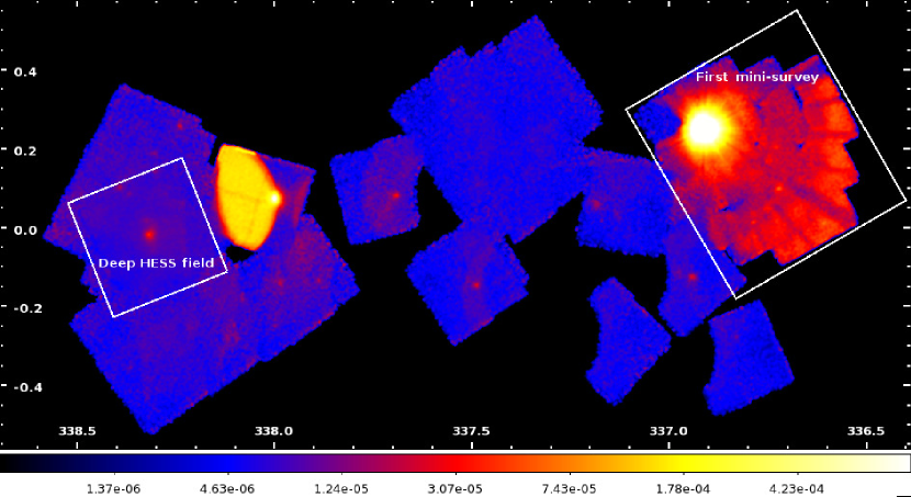
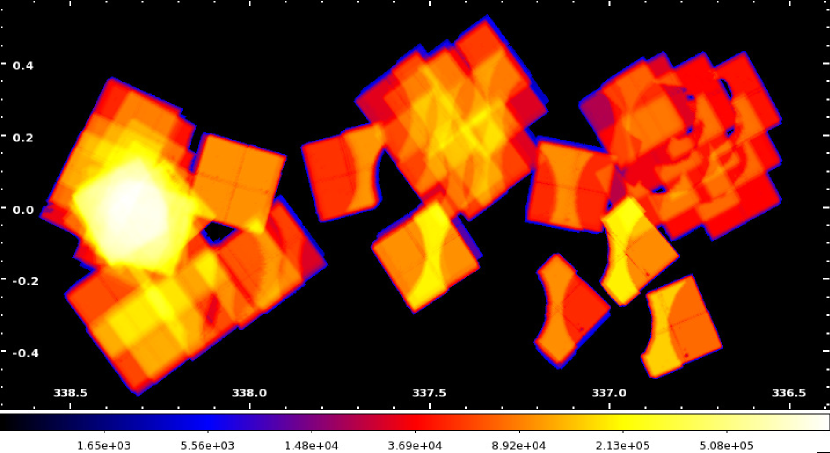
Figure 1.— The top panel shows the smoothed 3–40 keV count rate mosaic (units of counts per second) and the bottom shows the 3–40 keV exposure map without vignetting correction (units of seconds). The mosaics have been cleaned of most contamination from ghost rays and stray light; some residual ghost ray contamination can be seen in the first mini survey (upper right of the mosaic) while one wedge of stray light around ($\ell$, $b$) = (338^∘, 0.08^∘), which is due to GX 340+0, is not removed since a bright source, IGR J16393-4643, is embedded in it.

II.2. Chandra

In this study, we make extensive use of information from the Norma Arm Region Chandra Survey (NARCS) catalog as well as the soft ($<10$ keV) X-ray spectra of some of the NARCS sources. The analysis of these Chandra observations and the details of the spectral extraction are provided in F14. We also use two other archival Chandra observations that cover part of the area surveyed by NuSTAR: ObsID 7591 provides an additional epoch for a transient source (NuSTAR J164116-4632.2, discussed in § V.5), and ObsID 11008 provides spatially resolved observations of NARCS sources 1278 and 1279 (Rahoui et al., 2014), which are blended in the NARCS and NuSTAR Norma observations. For reference, we provide information about all these relevant archival Chandra observations in Table 2.

Furthermore, in this study we make use of Chandra observations which were triggered to follow-up four transient sources discovered by NuSTAR. These Chandra observations were used to constrain their soft X-ray spectra and better localize their positions so as to be able to search for optical and infrared counterparts. The follow-up observations of one of these transients, NuSTAR J163433-4738.7, are discussed in T14, and the others are presented in § V.5 and listed in Table 3.

III. NuSTAR Data Processing and Mosaicking

The raw data of each observation was processed using CALDB v20150612 and the standard NuSTAR pipeline v1.3.1 provided under HEASOFT v6.15.1 to produce event files and exposure maps for both focal plane modules. We made exposure maps with and without vignetting corrections to be used in different parts of our analysis.

Next, we cleaned the event files of stray light contamination by filtering out X-ray events in stray light affected regions. Table LABEL:tab:obs indicates whether stray light removal occurred in either FPMA or FPMB as well as the source responsible for the stray light. In one exceptional case, we did not remove stray light seen in FPMA and FPMB of observation 30001008002, since a bright source, IGR J16393-4643, is located within the stray light regions caused by GX 340+0 and 4U 1624-49. We also excised the most significant ghost rays from observations from the first mini-survey, defining the ghost ray pattern regions in the same way as B14. One observation, 30001012002, was performed to follow-up NuSTAR J163433-4738.7, a transient source discovered in the first mini-survey; this observation helped to characterize the outburst duration of this transient (T14), but it was so extensively contaminated by ghost rays that it was not included in our analysis. Finally, a few observations show additional contamination features such as sharp streaks, listed in Table LABEL:tab:obs, which were also removed.

To improve the astrometric accuracy of the NuSTAR observations, we calculated the shifts between the positions of bright NuSTAR sources and their Chandra counterparts in NARCS observations which were astrometrically registered using infrared counterparts in the VISTA Variables in the Via Lactea (VVV; Minniti et al. 2010) survey (Fornasini et al., 2014). The positions of bright sources, which could be easily identified in raw images, were determined using the IDL gcntrd tool, which makes use of the DAOPHOT “FIND” centroid algorithm. This source localization was done independently for each FPM of each observation and was used to apply translational shifts to event files and exposure maps. In performing astrometric corrections, we limited ourselves to using sources with $>100$ net counts in each individual observation and FPM and located on-axis. For on-axis sources with this number of counts, we expect the statistical error on the centroid to be $<6^{\prime\prime}$ based on simulations (Brian Grefenstette, personal communication, May 7, 2014). NARCS 999 is very bright, with $>10,000$ net counts, and therefore the statistical uncertainties of the astrometric corrections derived from this source are $<2^{\prime\prime}$ at 90% confidence; the other sources used for astrometric corrections have $100-300$ net counts, and their associated statistical uncertainties are expected to be $5-6^{\prime\prime}$ at 90% confidence. Table 4 lists the applied boresight shifts and the bright sources used for astrometric correction. We were only able to apply these astrometric corrections to 23 out of 60 observations (43 out of 117 modules) due to the dearth of bright X-ray sources in our survey. Our inability to astrometrically correct all the observations does not significantly impact the results of our photometric and spectral analysis since the radii of the source regions we use are significantly larger than the expected shifts. The boresight shifts range from 1^′′ to 14^′′; 20% of the shifts are larger than 8^′′, which is more than expected based on NuSTAR’s nominal accuracy of $\pm$8^′′ at 90% confidence (Harrison et al., 2013), but is not unexpected given that the statistical errors on the source positions may be as high as 6^′′. Checking each shifted and un-shifted image by eye and comparing the locations of NuSTAR sources with their Chandra counterparts in shifted and un-shifted mosaic images, we confirm that these boresight shifts constitute an improvement over the original NuSTAR positions.

We re-projected the event files of each observation onto a common tangent point and merged all the observations and both FPM together to maximize photon statistics. We then generated mosaic images on the common sky grid in the 3–78, 3–10, 3–40, 10–20, 10–40, 20–40, and 40–78 keV bands. To create mosaic exposure maps, we combined the individual exposure maps by adding exposure values at the location of each sky pixel in the mosaic image; we made exposure maps both without vignetting corrections and with vignetting corrections evaluated at 8, 10, and 20 keV. We used the exposure maps without vignetting corrections when we calculated the source significance and net counts, since these calculations require comparing the exposure depth in the source and background region apertures and the background is dominated by non-focused emission. Instead, when calculating sensitivity curves (§ VI.2), we used exposure maps with vignetting corrections since the source emission is focused by the telescope mirrors. When calculating the source fluxes, vignetting corrections are taken into account through the ancillary response file (ARF). An exposure-corrected NuSTAR mosaic image in the 3–40 keV band and exposure map without vignetting correction are shown in Figure 1. As can be seen, the typical exposure depth of the Norma survey is 30–100 ks while the exposure of the deep field is 1 Ms.

IV. Source Detection

IV.1. Generating trial maps

To identify sources in the NuSTAR Norma survey, we employed a technique that was specifically developed for the NuSTAR surveys. This technique, which we refer to as the “trial map” technique, is described in detail by Hong et al. (2016), so we only provide a brief explanation here. The NuSTAR Galactic Center region survey (Hong et al., 2016), and the NuSTAR extragalactic surveys (Civano et al. 2015; Mullaney et al. 2015; Lansbury et al., submitted) all use this technique as the basis for their detection method. As a result of NuSTAR’s point spread function (PSF) being larger and its background being higher and more complex compared to other focusing X-ray telescopes such as Chandra and XMM-Newton, the utility of typical detection algorithms, such as wavdetect (Freeman et al., 2002), is limited when applied to NuSTAR data. One way of dealing with this problem is to add an additional level of screening to the results of conventional algorithms, calculating the significance of detections by independent means and setting a significance detection threshold. The trial map technique is more direct, skipping over the initial step of using a detection algorithm such as wavdetect.

To make a trial map, for each sky pixel, we calculate the probability of acquiring more than the total observed counts within a source region due to a random background fluctuation. For each pixel, the source and background regions are defined as a circle and an annulus, respectively, centered on that pixel. The mean background counts expected within the source region are estimated from the counts in the background region scaled by the ratio of the areas and exposure values of the source and background regions. Using background regions that are symmetric around the central pixel helps to account for spatial variations of the background. In making trial maps, we plot the inverse of the random chance probability, which is the number of random trials required to produce the observed counts simply by random background fluctuations, such that brighter sources with higher significance have higher values in the maps.

We generated trial maps using three different source region sizes with radii of $9\farcs 5$, 12^′′, and 17^′′ (corresponding to 15, 22, and 30% enclosures of the PSF, respectively) and six different energy bands (3–78, 3–10, 10–40, 40–78, 10–20, 20–40 keV). The source region sizes we used are slightly larger than those used in the analysis of the NuSTAR Galactic Center survey since the smaller sizes are especially suited for picking out relatively bright sources in areas of diffuse emission, but in the Norma region there is no evident diffuse emission apart from stray light and ghost rays. The inner and outer radii of the background regions are 51^′′ (corresponding to 70% of the PSF) and 85^′′ (equal to 5/3 of the inner radius), respectively, in all cases . Figure 2 shows trial maps made using the 22% PSF enclosure and the 3–10, 10–20, and 20–40 keV bands; the three energy bands are combined into a three-color image so that spectral differences between sources can be seen.

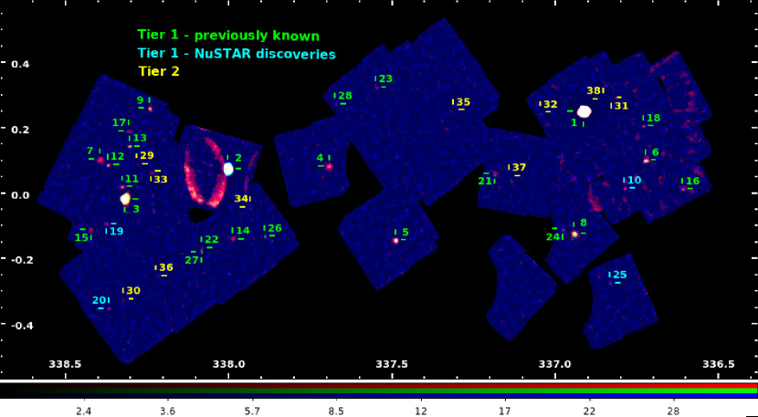
Figure 2.— Composite trial map showing the 3–10 keV band in red, 10–20 keV band in green, and 20–40 keV band in blue. The colors are scaled by the logarithmic trial map values. Tier 1 sources are labeled in green, if they were observed by NARCS or were previously well-studied, or cyan, if they were discovered by the NuSTAR Norma survey. Tier 2 sources are labeled in yellow. The streaks in the vicinity of NNR 2 are due to stray light which has not been removed because NNR 2 is partially embedded in it. The small streaks seen in the area covered by the first mini-survey are due to ghost rays from NNR 1.

IV.2. Detection Thresholds and Source Selection

When considering how to set detection thresholds for our trial maps, we excluded the observations from the first mini-survey and observation 30001008002 since they have significantly higher levels of stray light and ghost ray contamination than the rest of the survey; in the remainder of this paper, we will refer to this subset of observations as the “clean” sample. Figure 3 shows the fractional distributions of the values from the “clean” trial maps using source region sizes of 22% PSF enclosures. As can be seen, the distribution for the 40–78 keV band is very close to that expected for a Poissonian distribution of random background fluctuations, and in fact no sources are clearly visible in the “clean” trial maps.

Following the procedure described in Hong et al. (2016) to establish detection thresholds, we began by cross-correlating each trial map with the NARCS source catalog. Figure 4 shows the maximum trial map value within 10^′′ of the locations of NARCS sources detected at $>3\sigma$ in the 2–10 keV band as a function of Chandra photon flux. Above Chandra fluxes of $6\times 10^{-6}$ cm^-2 s^-1, more than 1/3 of NARCS sources have trial map values which are significantly higher than the bulk of NARCS sources clustered between trial map values of 10^0.3 to 10³. For Chandra fluxes lower than $2\times 10^{-6}$ cm^-2 s^-1, the distribution of trial map values are uncorrelated with source flux, having a linear Pearson correlation coefficient $|p|<0.04$ for all trial maps.

For a source to be considered for the final catalog, we require that it exceed the detection threshold in at least two trial maps. If all 18 trial maps were independent of each other, the expected number of false sources ($N_{\mathrm{F}}$) would be equal to $N_{\mathrm{can}}C(18,2)p^{16}(1-p)^{2}$, where $N_{\mathrm{can}}$ is the number of NARCS sources included in a NuSTAR counterpart search, $C(i,j)$ is a binomial coefficient, and $p$ is the fraction of false sources to be rejected in each map (Hong et al., 2016). However, the trial maps are not completely independent given that their energy ranges overlap. Thus, to at least partly account for the fact that some of the trial maps are correlated, we set a stringent limit on the expected number of false sources, setting $N_{\mathrm{F}}$=0.5. Since the long-term variability of NARCS sources is unknown, we search for NuSTAR detections among all NARCS sources. Thus, in the “clean” map regions, $N_{\mathrm{can}}$=579; limiting $N_{\mathrm{F}}$ to 0.5 requires a rejection percentage $p=99.76$%. Making a cumulative distribution function of the trial map values of uncorrelated NARCS sources lying in the gray area of Figure 4, we determine the corresponding trial value threshold for each trial map; the detection thresholds range from 10^5.2 in the 20–40 keV band with 15% PSF enclosures to 10^10.3 in the 3–10 keV band for 30% PSF enclosures.

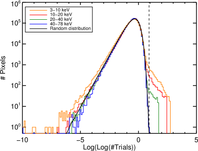
Figure 3.— Distribution of trial map values in different energy bands for 22% PSF enclosures. The x-axis is shown in a double logarithmic scale. The 40–78 keV distribution closely matches the random distribution expected due to Poissonian fluctuations of the background; this is consistent with the fact that among the “clean” observations included in creating this plot, only one source is detected in the 40–78 keV band. The vertical dashed line shows the detection threshold set for the 3–10 keV band trial map. The excess of high trial map values relative to the 40–78 keV band distribution is due to the presence of sources, stray light, and ghost rays; the excess of low trial map values result from the vicinity of bright sources, which effectively increase the local background.

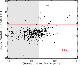
Figure 4.— Trial map value in the 3–10 keV band using 22% PSF enclosures versus Chandra 2–10 keV photon flux for NARCS sources in the surveyed NuSTAR area. Fluxes of sources in the gray region are uncorrelated with the trial map values and used to set the detection threshold, which is shown by the red horizontal line. Sources above the horizontal line in at least two trial maps are tier 1 sources, while bright sources below that line but to the right of the vertical dashed line are tier 2 candidates.

Having established detection thresholds for each trial map, we first searched for any Chandra sources detected by NuSTAR. We cross-correlated all NARCS sources detected at $>3\sigma$ in the 2–10 keV Chandra band with the trial maps of the full set of observations, including those with significant background contamination. We considered all NARCS sources that exceed the detection threshold in at least two trial maps as tier 1 candidate sources. All sources with 2–10 keV Chandra flux $>6\times 10^{-6}$ cm^-2 s^-1 that are not tier 1 sources are considered tier 2 candidate sources, regardless of their trial map values. Although for tier 2 sources, we do not expect to be able to retrieve significant spectral information, we can at least check for significant variability between the Chandra and NuSTAR observations and place upper limits on the flux above 10 keV. We also performed a blind search for NuSTAR sources that were not detected in NARCS; we consider any clusters of pixels that exceed the detection threshold in at least three trial maps as additional tier 1 candidate sources.

We then inspected all the candidate sources. First, we checked whether NuSTAR sources matched to Chandra counterparts are unique matches. We find 13 cases in which multiple NARCS sources were associated with a single NuSTAR detection due to NuSTAR’s much larger PSF; however, in all these cases, one NARCS source was more clearly centered on the NuSTAR position and was also significantly brighter, demonstrating the more likely association. We then visually inspect all tier 1 candidate sources without NARCS associations to ensure they are not associated with artifacts due to stray light, ghost rays, or the edges of the fields of view (FoVs). Based on this visual inspection, we exclude three candidate sources located at the edges of the FoVs, the stray light region near NNR 2, and 21 candidates without a clear point-like morphology that are located in the first mini-survey area contaminated by ghost rays. In addition, since tier 2 candidate sources do not exceed the trial map detection thresholds, in order for them to be included in our final catalog, we require that their aperture photometry have a signal-to-noise ratio (S/N)$>3\sigma$ in at least one of the 3–10, 3–40, or 10–20 keV energy bands (see § V.2 for details). In total, after these different screenings, 28 tier 1 candidates and 10 tier 2 candidates are included in our final source list, shown in Table LABEL:tab:srclist.

To determine the best position of tier 1 NuSTAR sources, we applied the DAOPHOT “FIND” algorithm in the proximity of each source in the 3–10 keV trial map with 22% PSF enclosure; we found that using the centroid algorithm on the trial maps rather than the mosaic images yielded better results, allowing the algorithm to converge for all tier 1 sources with lower statistical errors. When applying the centroid algorithm, we used the 3–10 keV, 22% PSF trial map since all the tier 1 sources are clearly discernible in this map. The tier 2 sources are not bright enough for the centroid algorithm to yield reliable results, so we simply adopt the Chandra positions for these sources. The offsets between tier 1 sources and their Chandra counterparts vary from $0\farcs 9$ to 14^′′, excluding two extended sources (NNR 8 and 21) whose Chandra positions were determined subjectively by eye. The offsets of four NuSTAR point sources from their Chandra counterparts are larger than the 90% NuSTAR positional uncertainties. We estimated the NuSTAR positional uncertainty for each tier 1 source as the quadrature sum of statistical and systematic uncertainties. We calculated the statistical error by performing Gaussian fits to histograms of the spatial count distributions in the X and Y directions in a $25\times 25$ pixel image cutout centered on the source position. These statistical errors are approximate since the NuSTAR PSF has non-Gaussian wings, but comparison of the errors derived using the Gaussian approximation to those derived from the accurate PSF simulations performed for some of the brighter sources (see §III) indicates this approximation is accurate to 10%. For the systematic uncertainty, we assumed the nominal $8^{\prime\prime}$ astrometric accuracy (Harrison et al., 2013) for sources located in observations which were not astrometrically corrected and the uncertainties calculated in §III for sources in astrometrically-corrected observations. Looking carefully at the four sources with the largest offsets, the similarity between their fluxes and/or spectral properties in the 2–10 keV band between Chandra and NuSTAR suggests that they are true counterparts despite the large positional offsets. The fact that 17% of the NuSTAR offsets exceed the 90% positional uncertainties suggests that the NuSTAR positional uncertainty is slightly underestimated. Large offsets between NuSTAR positions and soft X-ray counterparts are also seen in the NuSTAR serendipitous survey, where Lansbury et al. (2016) find that the 90% positional accuracy of NuSTAR varies from 12^′′ for the most significant detections to 20^′′ for the least significant detections. The large NuSTAR offsets in the serendipitous survey suggest that the 90% NuSTAR systematic uncertainty is larger than 8^′′, which would help to explain some of the large offsets seen for sources in the Norma survey.

Table LABEL:tab:srclist provides information about the detection, position, and Chandra counterparts of all NuSTAR Norma region (NNR) sources. The tier 1 sources include five sources not detected in NARCS; one of them is the well-known LMXB 4U 1630-472 (Kuulkers et al., 1997) while the others are new transient sources discussed in § V.5.

V. Aperture Photometry

V.1. Defining source and background regions

For photometry and spectral extraction, we used circular source regions and, whenever possible, annular background regions centered on the source positions provided in Table LABEL:tab:srclist. At energies below 20 keV, the NuSTAR background is not uniform as it is dominated by non-focused emission, which exhibits spatial variations due to shadowing of the focal plane (Harrison et al., 2013). Using aperture regions that are symmetric about the source position helps to compensate for this non-uniformity. We performed our photometric analysis with two different source extraction regions with 30^′′ and 40^′′ radii (corresponding to roughly 50% and 60% PSF enclosures, respectively), to assess possible systematic errors associated with aperture selection. The default background regions are annuli with 60^′′ inner radii and 90^′′ outer radii. For NNR 8 and 21, which appear extended and are not fully contained within the default source regions, we adopted radii of 45^′′ and 60^′′ for the small and large circular source regions, respectively, and annular background regions with 80^′′ inner radii and 110^′′ outer radii. We adjusted the centers of the aperture regions for NNR 8 and 21 by 8^′′ and $5^{\prime\prime}$, respectively, so that they were more centered with respect to the full extended emission rather than the peak of the emission .

For about 1/3 of sources, it was necessary to modify the background aperture regions. In order to prevent contamination to the background from other sources, it is preferable for background regions not to extend within 60^′′ of any tier 1 source. In addition, above 20 keV, as the relative contribution of the internal background becomes more significant, the background is fairly uniform across any given detector but differs between detectors (Harrison et al. 2013; Wik et al. 2014), so it is advantageous for the background region to be located on the same detector as the source region. Furthermore, when a source is located close to the edge of the field of view, using an annular background region may not sample a statistically large enough number of background counts. Finally, although we removed the most significant patches of stray light and ghost ray contamination from NuSTAR observations, non-uniform low-level contamination remains. Thus, we modified the background region in situations where the default background region comes within 60^′′ of any tier 1 source, the low-level contamination from stray light or ghost rays appears to differ significantly between the source and default background regions, or $>50\%$ of the annular background region falls outside the observation area or on a detector different from the one where the source is located. In these cases, we adopted a circle with a 70^′′ radius for the background region and placed it in as ideal a location as possible following these criteria:

• i. Keeping the region as close to the source as possible to minimize variations due to background inhomogeneities, but at least 60^′′ away from the source and any tier 1 sources.
  ii. Maximizing the fraction of the background region area that falls on the same detector as the source region.
  iii. Placing the background region at a location that exhibits a similar level of low-level stray light or ghost ray contamination as the source region.

For a given source, background aperture regions were defined for each observation and FPM individually since stray light and ghost ray contamination as well as the fraction of the default annular background that lies on a given detector varies depending on the observation and the module. Furthermore, if a source fell close to the edge of an observation, such that $>$50% of the area of a 40^′′ radius source region was outside the observation area, that observation was not used to extract photometric or spectral information for the source. Thus, the exposure value at the location of a source in the mosaicked exposure map may be higher than the effective exposure for the source based only on observations used for photometric analysis; the latter effective exposure is the value reported in Table LABEL:tab:srclist. Table LABEL:tab:phot provides the results of our aperture photometry and includes flags that indicate which sources required modified background regions.

The only exceptions to this method of defining background regions are NNR 22 and 27. These sources are only separated by 47^′′ and thus contaminate each other’s default background regions although they do not suffer from any additional background problems. Therefore, since annular background regions are preferable for minimizing vignetting effect, we simply redefined their background regions as an annulus with an 80^′′ inner radius and 110^′′ outer radius centered in between the two sources. Due to their proximity, the photometric and spectral properties of these sources as derived from 40^′′ radius circular apertures are less reliable than those from the 30^′′ radius apertures.

V.2. Net counts and source significance

Having defined aperture regions, we extracted the source and background counts for each source in each observation. We then calculated the expected number of background counts ($\langle c_{\mathrm{bkg}}\rangle$) in each source region by multiplying the counts in the background region by the ratio $(A_{\mathrm{src}}E_{\mathrm{src}})/(A_{\mathrm{bkg}}E_{\mathrm{bkg}})$, where $A_{\mathrm{src}}$ and $A_{\mathrm{bkg}}$ are the areas, in units of pixels, and $E_{\mathrm{src}}$ and $E_{\mathrm{bkg}}$ are the exposures (without vignetting corrections) of the source and background regions, respectively. Then for each source, we summed the source counts ($C_{\mathrm{src}}$), total background counts ($C_{\mathrm{bkg}}$), background counts expected in the source region ($\langle C_{\mathrm{bkg}}\rangle$), and exposures across all observations and modules in 7 different energy bands: 3–78, 3–40, 40–78, 3–10, 10–40, 10–20, and 20–40 keV. The 1$\sigma$ errors in the total counts were calculated using the recommended approximations for upper and lower limits in Gehrels (1986). Then, the net source counts ($C_{\mathrm{net}}$) were calculated by subtracting the total expected background counts in the source region from the total source counts.

In each energy band, we then calculated the signal-to-noise ratio (S/N) of the photometric measurements from the probability that the source could be generated by a noise fluctuation of the local background using the following equation from Weisskopf et al. (2007):

$$P(\geq C_{\mathrm{src}}|C_{\mathrm{bkg}};C_{\mathrm{net}}=0)=\\ \sum_{c=C_{\mathrm{src}}}^{C_{\mathrm{bkg}}+C_{\mathrm{src}}}\frac{(C_{\mathrm{bkg}}+C_{\mathrm{src}})!}{c!(C_{\mathrm{bkg}}+C_{\mathrm{src}}-c)!}\left(\frac{f}{1+f}\right)^{c}\left(1-\frac{f}{1+f}\right)^{C_{\mathrm{bkg}}+C_{\mathrm{src}}-c}$$ (1)

where $f=\langle C_{\mathrm{bkg}}\rangle/C_{\mathrm{bkg}}$. Using this probability, we define the S/N as the equivalent Gaussian significance in units of the standard deviation (e.g., $P=0.0013$ corresponds to S/N$=3\sigma$). These S/N measurements are used to select which tier 2 sources to include in our catalog, but not to set detection thresholds for tier 1 sources, which are determined by the trial maps. Only five sources have photometric measurements with S/N$\geq 3\sigma$ above 20 keV. Therefore, we focus the remainder of our analysis on the 3–40, 3–10, and 10–20 keV energy bands. Of the tier 2 source candidates, we only included those with S/N$\geq 3\sigma$ in at least one of these three energy bands, using either of the two source aperture regions, in our final source list. Table LABEL:tab:phot provides the significance of each source in our final catalog in these three energy bands, the net counts in the 3–40 keV band, and additional photometric properties described in the following sections. We estimate that local spatial variations of the background could affect the S/N values reported in this table by $\pm 0.4\sigma$, and change the measured net counts and fluxes by $\pm 5$%, variations which are smaller than the statistical uncertainties of the photometric measurements.

V.3. Photon and energy fluxes

In § V.7, we describe how we derived fluxes from spectral modeling, but for all sources we also derived fluxes in a model-independent way since the spectral fitting of faint sources is prone to significant uncertainty. For each source and background region in each observation and module, we used nuproducts to extract a list of photon counts as a function of energy and generate both an ARF and a response matrix file (RMF); the ARFs are scaled by the PSF energy fraction enclosed by the aperture region. We first calculated the source photon flux within each observation and module in the 3–10 and 10–20 keV bands by dividing the counts in each channel by the corresponding ARF, summing all these values within the given energy band, and then dividing by the source region exposure; the estimated background contribution, scaled from the photon flux measured in the background region, was subtracted. These photon flux measurements assume a quantum efficiency of 1, which is a decent approximation for the NuSTAR CdZnTe detectors, which have a quantum efficiency of 0.98 over the vast majority of the NuSTAR energy range (Bhalerao, 2012). If the significance of a source in a particular observation was $<1\sigma$, then we calculated a 90% confidence upper limit to its photon flux by converting the probability distribution of true source counts (from Equation A21 in Weisskopf et al. 2007) to a photon flux distribution using the source region effective area.

For the five transient sources which were detected by NuSTAR but not by NARCS, we looked at lightcurves of their 3–10 keV photon fluxes to check whether they are detected at $>2\sigma$ confidence in individual NuSTAR observations. We found that NNR 1 is only detected in ObsIDs 40014008002 and 40014009001, NNR 10 is only detected in ObsID 40014007001 (which is consistent with T14), and NNR 19 is only detected in ObsIDs 30002021005, 30002021007, 30002021009, 30002021011, and 30002021013. Excluding the observations in which the transient sources are not detected, we re-evaluated their 3–40 keV net counts and source significance as described in § V.2, and continued to exclude these observations for these sources when determining their other average photometric and spectral properties. Thus, the photometric and spectral properties derived for NNR 1, 10, 19, and 25 should be considered as their average properties during high flux states.

For each source, we then computed average 3–10 and 10–20 keV photon fluxes by combining the count lists and ARFs from different observations and modules. These measurements are presented in Table LABEL:tab:phot. We also calculate the average 3–10 and 10–20 keV energy flux for each source using the same model-independent method but with the additional step of multiplying the source counts in each channel by the channel energy. Fluxes derived using the two different source region sizes are in $1\sigma$ agreement with one another, except for three sources which are located in regions of diffuse emission or ghost rays and thus do not appear as exactly point-like. Comparing the model-independent fluxes with those we derived from spectral modeling (see § V.7) for tier 1 sources, we find they are in good agreement when using the smaller aperture regions, but show a significant number of discrepancies at $>2\sigma$ confidence when using the larger aperture regions. In the larger aperture regions, while the net number of source counts is higher, so is the background/source count ratio, which is why in most cases the source significance derived from the larger aperture regions is slightly lower; as a result, accurate background subtraction is more important when using the larger aperture regions and it is not surprising that our crude subtraction method, which assumes a spectrally flat background, for the model-independent fluxes leads to discrepancies with the spectral fluxes.

V.4. X-ray variability

NuSTAR’s high time resolution allows us to characterize the timing properties of detected sources over a range of timescales. NuSTAR’s time resolution is good to $\sim 2$ ms rms, after being corrected for thermal drift of the on-board clock, and the absolute accuracy is known to be better than $<3$ ms (Mori et al. 2014; Madsen et al. 2015). For our timing studies, all photon arrival times were converted to barycentric dynamical time (TDB) using the NuSTAR coordinates of each point source.

To characterize the source variability on $\sim\mathrm{hourly}$ timescales we used the Kolmogorov-Smirnov (KS) statistic to compare the temporal distributions of X-ray events extracted from source and background apertures in the $3-20$ keV energy band. The background light curve acts as a model for the count rate variations expected in the source region due to the background. The maximal difference between the two cumulative normalized light curves gives the probability that they are drawn from the same distribution, i.e. that the light curve in the source region is consistent with that expected from the background plus a source with constant flux. Any source with a KS statistic lower than $0.05\%$ in any observation is flagged as short-term variable by an “s” in Table LABEL:tab:phot. For each source, we ran the KS test independently for each of the observations in which it was covered. Since the KS test is applied 160 times in total, the adopted threshold corresponds to $\lesssim 1$ spurious detection. We identify two sources as variable using the KS test. An examination of the lightcuves of these sources, NNR 2 (presented in B16) and NNR 15 (Figure 5), shows clear variability on $\sim$hourly timescales.

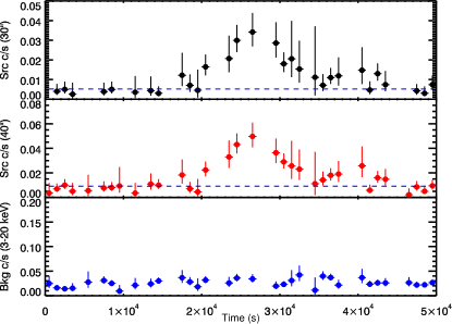
Figure 5.— Light curve of NNR 15 in the NuSTAR 3–20 keV band from ObsID 40014016001, FPMA and FPMB combined, as measured from an aperture region with a 30^′′ radius (top) and a 40^′′ radius (middle). The light curve exhibits evident short-term variability. The bottom panel displays the light curve extracted from the background aperture region; the blue dashed lines in the top two panels show the mean background count rate scaled by the source region area. The light curves display the average count rate in each 1 ks time interval; note that during some of these time intervals, the effective exposure time is less than 1 ks due to Earth occultations or periods of poor data quality.

We checked for variability of the NNR sources on week to year timescales by comparing the flux detected between repeated NuSTAR observations. Sources were flagged as long-term variable with an “l” in Table LABEL:tab:phot if their $3-10$ keV photon flux differed by $>3\sigma$ based on their flux measured uncertainties; given the number of flux comparisons performed, this $3\sigma$ threshold should result in $\lesssim 1$ spurious detection. NNR 1, 10, 11, 19, and 29 were found to be variable using this criterion. In addition, we compared Chandra and NuSTAR fluxes to check for variability on year timescales. For all sources with sufficient photon statistics, we compared the joint spectral fits to Chandra and NuSTAR data (see § V.7 for details), and identified sources with normalizations that differed at the $>90$% confidence level. Since we performed these joint fits for 24 sources, we would expect as many as two spurious detections of variability, but we made the criterion more stringent by requiring that for a source to be considered variable between the Chandra and NuSTAR observations, its Chandra and NuSTAR normalizations must be inconsistent regardless of which of three different spectral models is adopted. This more selective criterion is only met by NNR 4, 11, and 27. For fainter sources (NNR 29-38), we considered a range of spectral models that would be consistent with their quantile values, and assessed whether their 2–10 keV Chandra flux was incompatible with their average 3–10 keV NuSTAR flux at $>90$% confidence, regardless of the spectral model assumed. NNR 28, 35, and 36 are found to be variable by this criterion. In Table  7, we provide maximum photon fluxes and the ratio of maximum and minimum fluxes for all NuSTAR sources that demonstrate X-ray variability; the transient sources, NNR 1, 10, 19, 20, and 25, which are detected by NuSTAR but not detected in NARCS, are flagged as long-term variable and included in this table as well.

We searched for a periodic signal from those NuSTAR sources with sufficient counts to detect a coherent timing signal, determined as follows. The ability to detect pulsations depends strongly on the source and background counts and number of search trials. For a sinusoidal signal, the aperture counts (source plus background) necessary to detect a signal of pulsed fraction $f_{p}$ is $N=2S/f^{2}_{p}$, where $S$ is the power associated with the single trial false detection probability of a test signal $\wp=e^{-S/2}$; $S$ is distributed as $\chi^{2}$ with two degrees of freedom (van der Klis, 1989). In practice, for a blind search, we need to take into account the number of frequencies tested $N_{trials}=T_{span}/f_{Nyq}$, when $T_{span}$ is the data span and $f_{Nyq}=250$ Hz, the effective NuSTAR Nyquist frequency. In computing $N$ we must allow for the reduced sensitivity of the search due to background contamination in the source aperture ($N_{b}$); the minimum detectable pulse fraction $f_{p}({\mathrm{min}})$ is then increased by $(N_{s}+N_{b})/N_{s}$.

We computed the detectability in individual observations for each source in our sample and considered those suitable for a pulsar search, with $f_{p}({\mathrm{min}})>50\%$ at the $3\sigma$ level. For the three brightest sources in the Norma survey, their timing properties are already presented elsewhere: i) the quasi-periodic oscillations of the black hole binary 4U 1630- 472 (NNR 1) were extensively studied using the Rossi X-ray Timing Explorer (Tomsick & Kaaret 2000; Dieters et al. 2000; Seifina, Titarchuk & Shaposhnikov 2014), ii) the high mass X-ray binary pulsar HMXB IGR J16393-4643 (NNR 2) with a period of 904 seconds, whose spin-up rate was determined from recent NuSTAR observations (B16), and iii) the NuSTAR-discovered 206 ms pulsar PSR J1640$-$4631 (NNR 3) associated with the TeV source HESS J1640$-$465 (G14;Archibald et al. 2016).

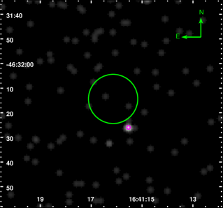
(a) NNR 19, Chandra ObsID 16170

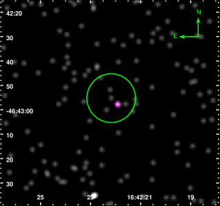
(b) NNR 20, Chandra ObsID 16171

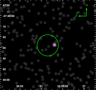
(c) NNR 25, Chandra ObsID 17242

Figure 6.— Chandra follow-up observations of NuSTAR transients in the 0.5–10 keV band (see Table 3). NuSTAR source positions are shown with 90% confidence error circles in green, and the locations of the nearest Chandra sources are indicated with 90% confidence error circles in magenta. The NuSTAR and Chandra positional uncertainties are provided in Tables LABEL:tab:srclist and 8, and are approximately 10^′′ and 0$\farcs$7, respectively, for all three sources.

For NNR 4, 5, 8, and 21, we extracted event lists in the $3-20$ keV band from $r=40^{\prime\prime}$ radius apertures and searched for periodic signals between 4 ms and 100 seconds. For each source, we evaluated the power at each frequency (oversampling by a factor of two) using the unbinned $Z^{2}_{n}$ test statistic (Buccheri et al., 1983) summed over $n=1,2,3,5$ harmonics, to be sensitive to both broad and narrow pulse profiles. We repeated our search for an additional combination of energy ranges $3<E<25$ keV, $3<E<10$ keV, $10<E<25$ keV, $10<E<40$ keV, and aperture size $r<20^{\prime\prime}$ and $r<30^{\prime\prime}$. For all these searches, no significant signals were detected. For NNR 5 and 8, we can constrain the pulsed fraction of X-ray emission to be $<45\%$ and $<48\%$, respectively, at the $3\sigma$ confidence. We also performed periodic searches for longer periods, with special attention to NNR 4 for which Chandra detected a 7150 second period, but we were unable to pick out any signals that could clearly be attributed to the NuSTAR sources due to the artifacts introduced by NuSTAR’s orbital occultations to the Fourier power spectrum.

V.5. Chandra follow-up of NuSTAR discoveries

As discussed in § II, we triggered Chandra follow-up observations for the four sources discovered by NuSTAR, NNR 10, 19, 20, and 25. NNR 10, 19, and 25 were not detected by NARCS despite its much higher sensitivity compared to the NuSTAR Norma survey, indicating these are transient sources. NNR 20 falls outside the area surveyed by Chandra, but our follow-up Chandra observations show that its flux is also highly variable.

The analysis of the Chandra follow-up of NNR 10 is presented in T14, while the analysis of the other three observations, which are listed in Table 3, is described here. The archival Chandra observation 7591 (see Table 2, which provides additional coverage of NNR 19) was also subjected to the same analysis. The Chandra observations were processed using CIAO version 4.7 adopting standard procedures. Then we used wavdetect to determine the positions of Chandra sources in the vicinity of the NuSTAR sources. The statistical uncertainties of the Chandra positions were calculated using the parametrization in Equation 5 of Hong et al. (2005); the 90% statistical uncertainty was then combined with Chandra’s $0\farcs 64$ systematic uncertainty in quadrature. Since NNR 19 was also detected in an archival Chandra observation, we averaged the positions determined from ObsIDs 7591 and 16170. The Chandra positions and uncertainties are reported in Table 8. The Chandra follow-up observations of NNR 9, 20, and 25 are shown in Figure 6, where green circles indicate the NuSTAR source positions and magenta circles show the locations of the nearest Chandra sources.

The closest Chandra source to NNR 19 is located at a distance of $13\farcs 2$, which is outside of the 90% confidence NuSTAR error circle. However, as noted in Table LABEL:tab:srclist, a few of the NARCS counterparts have similarly large offsets, suggesting that in some cases the systematic NuSTAR positional uncertainties may be underestimated. The fact that only three days elapsed between the NuSTAR and Chandra observations of NNR 19 strengthens the case that these sources are indeed associated. Furthermore, this Chandra source was detected in 2007 in Chandra ObsID 7591, but undetected in 2011 in ObsID 12508; the fact that this Chandra source is a transient boosts the probability that it is the counterpart of NNR 19.

The only Chandra source in the vicinity of NNR 20 lies within the NuSTAR error circle but is only detected at 2.9$\sigma$ confidence. NNR 20 was not covered by previous Chandra observations, including NARCS, so before our follow-up observation (ObsID 16171), we did not know whether this source was a transient or not; based on its NuSTAR 3–10 keV flux, we would have expected to detect at least 10 counts from its Chandra counterpart if it was persistent. Thus, even if it is not definite that the weak Chandra detection is truly the counterpart of NNR 20, the lack of any brighter Chandra sources proves NNR 20 is a variable source.

Follow-up observations of NNR 25 were performed 34 days after the NuSTAR observations, and a Chandra source is clearly detected within the NuSTAR error circle. This Chandra source was not detected during the 2011 NARCS observations; its transient nature boosts the probability that it is the true counterpart of the transient NNR 25. As was done by F14 for all the NARCS sources, we searched for infrared counterparts to the NuSTAR-discovered sources in the VVV survey. We did not find any infrared counterparts to NNR 19, 20, or 25 within the 95% uncertainty of the Chandra-derived positions.

In order to extract photometric and spectral information for each Chandra counterpart, we defined source aperture regions as circles with $2\farcs 5$ radii and background regions as annuli with 15^′′ inner radii and 44^′′ outer radii. As the counterpart of NNR 19 was at a larger angular offset from the Chandra aimpoint in ObsID 7591, and the Chandra PSF increases in size with angular offset, the circular source region used for this observation had a 5^′′ radius. For each source in each Chandra observation, we calculate the net 0.5–10 keV counts, detection significance, and quantile values (see § V.6), which are provided in Table 8.

V.6. Hardness ratio and quantile analysis

Since spectral fitting can be unreliable or impractical for faint sources, we use hardness ratios and quantile values (Hong, Schlegel & Grindlay, 2004) to probe and compare the spectral properties of NuSTAR sources. In order to reduce the level of background contamination and prevent the hardness ratios and quantile values from being skewed towards the values of the NuSTAR background, we opted to use the aperture regions with smaller radii to derive these spectral parameters. The hardness ratio for each source is calculated as $(H-S)/(H+S)$, where $H$ is the counts in the hard (10–20 keV) band and $S$ is the counts in the soft (3–10 keV) band. The NuSTAR hardness ratios are listed in Table LABEL:tab:phot.

While hardness ratios are the most widely used proxy for spectral hardness of faint X-ray sources, they are subject to selection effects associated with having to choose two particular energy bands and they do not yield meaningful information for sources which have zero net counts in one of the two energy bands. Therefore, we also calculated quantile values for each source in the 3–40 keV band; these values are the median energy $E_{50}$, $E_{25}$ and $E_{75}$, the energies below which 25% and 75% of the source counts reside, respectively. The latter energies were combined into a single quantile ratio ($QR$) which is a measure of how broad or peaked the spectrum is and is defined as $QR=3(E_{25}-E_{\mathrm{min}})/(E_{75}-E_{\mathrm{min}})$, where $E_{\mathrm{min}}$ is the lower bound of the energy band, 3 keV for NuSTAR and 0.5 keV for Chandra. The NuSTAR median energy and $QR$ value of each source is provided in Table LABEL:tab:phot and shown in Figure 7(a). The gridlines in this figure indicate where a source with a particular blackbody, bremsstrahlung, or power-law spectrum would fall in the NuSTAR quantile space; gridlines which are roughly vertical represent different temperatures ($kT$) or photon indices ($\Gamma$) while roughly horizontal gridlines represent different values of the absorbing column density along the line-of-sight to the source ($N_{\mathrm{H}}$).

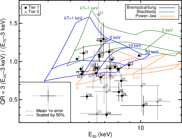
(a) NuSTAR quantile diagram.

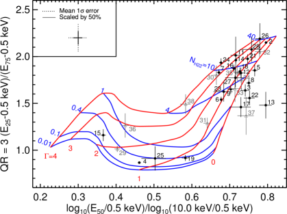
(b) Chandra quantile diagram.

Figure 7.— Quantile diagrams showing the quantile ratio on the y-axis and the median energy on the x-axis (or median energy “normalized” by the Chandra 0.5–10 keV band for the lower panel). Quantile values of tier 1 sources are shown with black circles and those of tier 2 sources are shown with gray trinagles. Comparing the positions of sources in the quantile diagrams to the spectral model gridlines provides a rough measurement of their spectral parameters. The Chandra quantiles are very sensitive to the amount of absorption suffered by a source, while the NuSTAR quantiles are more useful for separating sources with different spectral slopes. To improve the legibility of the plots, 1$\sigma$ error bars have been scaled down by 50%. As a visual aide, the corner boxes in each plot show the mean 1$\sigma$ uncertainty for the tier 1 sources and the same mean error scaled by 50%. (a) The NuSTAR 3–40 keV background has $E_{50}=$ 10–15 keV and $QR$ = 0.4–0.6, which is why several tier 2 sources, which are most affected by the background, are found near that position in the diagram. Grids representing absorbed bremsstrahlung, blackbody, and power-law models are shown in blue, green, and orange, respectively. Roughly vertical grid lines represent different values of the temperature ($kT$) or photon index ($\Gamma$). Primarily horizontal grid lines represent $N_{\mathrm{H}}=10^{22},10^{23},5\times 10^{23}$ cm^-2 from bottom to top. (b) A grid of a power-law spectral model attenuated by interstellar absorption is overlaid. Red (primarily vertical) lines represent values of the photon index $\Gamma=0,1,2,3,$ and 4 from right to left. Blue (primarily horizontal) lines represent values of the hydrogen column density $N_{\mathrm{H}}=0.01$, 0.1, 0.4, 1, 4, 10, and 40 in units of $10^{22}$ cm^-2 from bottom to top.

Figure 7(b) shows the quantile values of the Chandra counterparts of the NuSTAR sources in the 0.5–10 keV band. Most of these values are taken from the NARCS catalog (F14). The quantile values for Chandra counterparts of NNR 19 and 25 were derived using the aperture regions described in § V.5; the values for NNR 19 derived from ObsIDs 7591 and 16170 were combined in a weighted average. The Chandra counterpart of NNR 20 only has 3 counts, which are too few for quantile analysis; however, all three photons have energies $>4$ keV, indicating that this source is subject to significant absorption since Chandra’s effective area peaks below 2 keV. Finally, we did not adopt the NARCS catalog quantile values for extended sources, because they were derived using aperture regions whose position and extent were determined by eye and which removed embedded point sources not distinguishable with NuSTAR. Therefore, we recalculated the quantile values for extended sources using circular aperture regions with 45^′′-radii centered on the NuSTAR-determined positions of NNR 8 and 21; these Chandra quantiles are weighted averages of values derived from ObsIDs 12528 and 12529 for the counterpart of NNR 8 and ObsIDs 12523 and 12526 for the counterpart of NNR 21.

As can be seen in Figure 7, the Chandra quantiles can easily differentiate between foreground sources and those subject to high levels of absorption due to gas along the line-of-sight. The integrated column density of neutral and molecular hydrogen due to the interstellar medium along the line-of-sight in the Norma region varies from $4-9\times 10^{22}$ cm^-2, as derived from the sum of $N_{\mathrm{HI}}$ measured by the Leiden/Argentine/Bonn survey (Kalberla et al., 2005) and $N_{\mathrm{H_{2}}}$ estimated from the MWA CO survey (Bronfman et al., 1989) using the $N_{\mathrm{H_{2}}}/I_{\mathrm{CO}}$ factor from Dame, Hartmann & Thaddeus (2001); since these surveys have 0.5^∘ resolution, the interstellar $N_{\mathrm{HI+H_{2}}}$ values we derive are averages over 0.25 deg² regions, so it is possible that the interstellar absorption is actually higher or lower along particular lines-of-sight due to the clumpy nature of molecular clouds. Thus, the sources whose X-ray spectra show column densities in excess of these values may be located behind dense molecular clouds or suffer from additional absorption due to gas or dust local to the X-ray source. The NuSTAR quantiles are not particularly sensitive to $N_{\mathrm{H}}$, but instead are able to separate sources with intrinsically soft and hard spectra, regardless of their level of absorption. Thus, the combination of quantile values in the Chandra and NuSTAR bands allows us to learn a fair amount about the spectral properties of sources which are too faint for spectral fitting and provide a check on spectral fitting results which can depend on the choice of binning for low photon statistics.

V.7. Spectral Analysis

For all tier 1 sources with $>$100 net counts in the 40^′′ radius aperture in the 3–40 keV band, we perform spectral analysis using XSPEC version 12.8.2 (Arnaud, 1996), jointly fitting the NuSTAR and Chandra data when it is available. All spectral parameters were tied together for these joint fits, except for a cross-normalization factor between the Chandra and NuSTAR observations which was left as a free parameter to account for source variability and differences in instrumental calibrations (measured to be consistent to 10% precision, Madsen et al. 2015). We also included a cross-normalization constant between NuSTAR FPMA and FPMB in our models; for most sources, due to limited photon statistics, the errors on this normalization constant are large and the constant is consistent with 1.0 to better than 90% confidence. Thus, for the NuSTAR sources detected with lowest significance (i.e., with trial map values $<10^{15}$), we fixed the FPMA/B normalization constant to 1. To maximize the number of counts per spectral bin, we used the larger aperture source regions to extract information for spectral fitting; however, for NNR 22 and 27, which are only separated by 47^′′, we extracted spectral information from 30^′′ source regions to limit the blending of the two sources. The spectra of the Chandra counterparts were extracted as described in F14 for NARCS sources and § V.5 for the counterparts of NuSTAR discoveries; however, for the extended counterparts of NNR 8 and 21, we defined aperture regions as 60^′′-radius circles centered on the NuSTAR-derived position in order to match the NuSTAR extraction region.

The Chandra and NuSTAR spectra were grouped into bins of $>2-10\sigma$ confidence, depending on the net counts of each source. For the three brightest sources which have been carefully analyzed in other papers, we adopt simplified versions of the best-fitting models found in King et al. (2014), B16, and G14, in order to easily measure their observed and unabsorbed fluxes in the 3–10 and 10–20 keV bands which we use to calculate the log$N$-log$S$ distribution of our survey (§ VI.3). For other tier 1 sources, we fit absorbed power-law, bremsstrahlung, and collisionally-ionized models; we employed the tbabs absorption model with solar abundances from Wilms, Allen & McCray (2000) and photoionization cross-sections from Verner et al. (1996). When Fe line emission was clearly visible between 6.4 and 7.1 keV, we also included a Gaussian line in the spectral models. Due to NuSTAR’s 0.4 keV resolution at 6–7 keV enegies, multiple Fe lines would appear blended in our spectra, especially given the low photon statistics. Thus, measurements of the Fe line parameters should be interpreted as the average energy of the Fe line complex and the combined equivalent width of the Fe lines. If Fe line emission was not evident, the source spectrum was first fit without a Gaussian component. Then, having determined which of the three spectral models best fit the spectrum, a Gaussian component was added in order to place constraints on the strength of Fe line emission that may not be visible due to poor photon statistics. The central energy of this Gaussian component was constrained to be between 6.3 and 7.1 keV and its width was fixed to zero; we tested the effect of fixing the width to values as high as 0.1 keV, but the impact on the results was negligible. Then the 90% upper limit on the line normalization was used to calculate the 90% upper limit on the Fe line equivalent width. In addition, when significant residuals remained at soft energies, we introduced a partial covering model (pcfabs) to test if it provides a significant improvement of the chi-squared statistic. Including this component substantially improved $\chi^{2}$ for NNR 4 and 6, but for NNR 6 the $N_{\mathrm{H}}$ of the partial absorber could not be well constrained and the covering fraction was found to be consistent with 1.0 to 90% confidence. Thus, since the spectral quality of NNR 6 was not good enough to constrain the additional pcfabs component, we did not include it in our final model fit for NNR 6.

The results of our spectral analysis can be found in Table LABEL:tab:spectra, and the spectra and fit residuals are shown in Figure 8 and the appendix. As can be seen, spectra with $<300$ NuSTAR counts cannot place strong constraints on the spectral parameters. However, we nonetheless include these results to be able to compare non-parametric fluxes with spectrally derived fluxes, and as a reference to aid the design of future NuSTAR surveys.

We used the model fit with the best reduced chi-square statistic to determine observed energy fluxes for each source in the 2–10, 3–10, and 10–20 keV bands and conversion factors from photon fluxes to unabsorbed energy fluxes, which are listed in Table 10. These conversion factors are used to calculate the log$N$-log$S$ distribution for unabsorbed fluxes (see § VI.3). The faintest tier 1 source, NNR 28, does not have enough counts to permit spectral fitting; based on its quantile values, it has $N_{\mathrm{H}}\approx 10^{23}$ cm^-2 and $\Gamma\approx 1.8$. Fixing the parameters of an absorbed power-law model to these values while allowing the Chandra and NuSTAR normalizations to vary independently, we fit the unbinned spectra of NNR 28 using the C-statistic (Cash, 1979) and find a goodness of fit lower than 28%. The observed and unabsorbed fluxes of NNR 28 measured from these fits are included in Table 10.

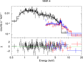
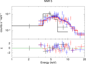
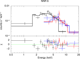
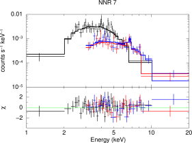
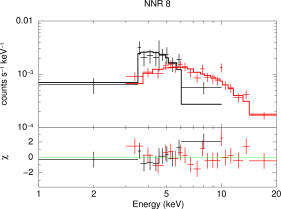
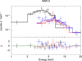
Figure 8.— Example Chandra and NuSTAR spectra with residuals of best-fitting model. Chandra data is shown in black, NuSTAR FPMA data is shown in red, and FPMB data is shown in blue. Additional spectra are shown in the appendix at the end of the paper. Spectral analysis results can be found in Table LABEL:tab:spectra.

To ensure that these results were not significantly dependent on the binning that was chosen, we compared the best-fitting parameters with those derived by fitting unbinned spectra using the C-statistic and the locations of sources in the quantile diagrams; no significant discrepancies were found except for sources with strong Fe lines, which is to be expected since the quantile grids do not account for the presence of Fe lines. However, for NNR 17, our analysis yields a harder spectrum than is found by B14. This source lies in the ghost ray pattern of 4U 1630-472, making background subtraction particularly challenging. The background region we selected contains higher ghost ray contamination than the background chosen by B14; we consider our selection more appropriate given that this source resides in a region of high ghost ray contamination. Since the spectrum of 4U 1630-472 is dominated by a blackbody component with $kT\approx 1.4$ keV, the fact that B14 measured a softer spectrum for NNR 17 than we do, with $\Gamma=3.7\pm 0.5$ rather than 2.0${}^{+1.0}_{-0.8}$, suggests that the background contribution from ghost rays may have been underestimated by B14. The photon index we measure is also more consistent with the hard photon index indicated by the Chandra quantiles (see Figure 7(b)).

VI. Discussion

VI.1. Classification of NuSTAR Sources

The X-ray spectral and timing properties of the NuSTAR sources, as well as information about their optical and infrared counterparts, can help identify their physical nature. The three brightest sources in the NuSTAR Norma survey are well-studied and classified; 4U 1630-472 (NNR 1) is a black hole LMXB (e.g. Barret, McClintock & Grindlay 1996; Klein-Wolt, Homan & van der Klis 2004), IGR J16393-4643 (NNR 2) is a neutron star HMXB (Bodaghee et al. 2006; B16), and HESS J1640-465 (NNR 3) is a pulsar and associated pulsar wind nebula (G14;Archibald et al. 2016). Here we present the most likely classifications of the fainter NuSTAR sources and their hard X-ray properties.

VI.1.1 Colliding wind binaries

Two of the NuSTAR sources in the Norma region are likely colliding wind binaries (CWBs), NNR 7 and 14.

NNR 7 actually consists of two Chandra sources blended together due to NuSTAR’s PSF. In Chandra ObsID 11008, where these two sources are resolved, they exhibit very similar spectral properties ($N_{\mathrm{H}}$ and $kT$ values are consistent at ¡1$\sigma$ level), but the 0.5–10 keV flux of NARCS 1279 is 2 times higher than the flux of NARCS 1278. These sources are blended in Chandra ObsIDs 12508 and 12509 because they are far off-axis, and the combined flux of the two sources is a factor of 3 higher in these later observations. Spectroscopic follow-up of the near-IR counterparts of both of these Chandra sources revealed they are Wolf-Rayet stars of spectral type WN8 (Rahoui et al., 2014). These stars belong to the young massive cluster Mercer 81 (Mercer et al., 2005) located at a distance of 11$\pm$2 kpc (Davies et al., 2012). The Chandra spectra of these sources were better fit by thermal plasma models than power-law models, suggesting that these sources were more likely to be CWBs than HMXBs with compact objects accreting from the powerful Wolf-Rayet stellar winds.

The NuSTAR data provides even stronger support for the CWB hypothesis for NNR 7. Joint fitting of the Chandra (from NARCS) and NuSTAR spectra of these blended sources reveal that they fall off steeply above 1  keV and show prominent Fe line emission, primarily due to Fe XXV based on its 6.76$\pm$0.1  keV line energy (House, 1969). The spectra are best fit by an apec thermal model with $kT=3.2^{+0.8}_{-0.5}$ keV and a metal abundance of 0.5$\pm$0.3 solar, or a steep power-law model with $\Gamma=3.4^{+0.4}_{-0.3}$ and Fe line emission with $650\pm 20$ eV equivalent width. These spectral properties rule out the possibility that NNR 7 could be an accreting HMXB, since accreting HMXBs have harder power-law spectra and Fe I K$\alpha$ emission at 6.4 keV, typically with equivalent widths $<100$ eV (Torrejón et al., 2010). Elshamouty, Heinke & Chouinard (2016) found that, in quiescence, one neutron star HMXB, V0332+53 exhibits a soft spectrum ($\Gamma\approx 4$ or $kT_{\mathrm{BB}}\approx 0.4$ keV) without prominent Fe lines; if this spectrum is typical of quiescent HMXBs, then we can also rule out the possibility that NNR 7 is a quiescent HMXB given its hard spectrum and prominent Fe emission. The unabsorbed 0.5–10 keV flux of NNR 7 based on the combined NARCS and NuSTAR spectrum is $1.20^{+0.04}_{-0.12}\times 10^{-12}$ erg cm^-2 s^-1. Adopting the 0.5–10 keV flux ratio for NARCS 1278 and 1279 and the bolometric luminosities of their Wolf-Rayet counterparts calculated by Rahoui et al. (2014), we find that their respective X-ray luminosities are $5\times 10^{33}$ erg s^-1 and $1.2\times 10^{34}$ erg s^-1, and they have $L_{X}/L_{\mathrm{bol}}=1.3\times 10^{-6}$ and $8\times 10^{-7}$, respectively.

Isolated high-mass stars are known to be X-ray emitters, but their spectra typically have $kT\sim 0.5$ keV and their 0.5–10 keV luminosities follow the scaling relation $L_{X}/L_{\mathrm{bol}}\approx 10^{-7}$ (e.g. Berghoefer et al. 1997; Sana et al. 2006). The harder X-ray emission and higher $L_{X}/L_{\mathrm{bol}}$ exhibited by NNR 7 have been observed from the wind-wind shocks in CWBs (Zhekov & Skinner 2000; Portegies Zwart, Pooley & Lewin 2002) and the magnetically channeled shocks of high-mass stars with $\sim$kG fields (Gagné et al. 2005; Petit et al. 2013). For NNR 7, a CWB nature is more likely given the strength of the Fe line at 6.7 keV; magnetic high-mass stars tend to exhibit weak Fe XXV line emission (Schulz et al. 2000; Schulz et al. 2003), while the Fe XXV lines in CWB spectra can have equivalent widths as large as $\sim 1-2$ keV (Viotti et al. 2004; Mikles et al. 2006). The X-ray spectrum of NNR 7 exhibits substantial absorption corresponding to $N_{\mathrm{H}}=1.1\pm 0.2\times 10^{23}$ cm^-2, which is in excess of the integrated interstellar absorption along the line-of-sight ($N_{\mathrm{HI+H_{2}}}=7.8\times 10^{22}$ cm^-2). The excess absorption measured in the X-ray spectrum of NNR 7 could either be due to inhomogeneities in the ISM or local absorption, which is observed in some CWBs, such as $\eta$ Carinae (Hamaguchi et al., 2007). Finally, X-ray variability is more common in CWBs than isolated high-mass stars (Corcoran, 1996). The X-ray flux variations displayed by CWBs are primarily associated with the orbital period of the binary and can be as large as a factor of $\approx 20$ (Pittard et al. 1998; Corcoran 2005). Thus, the X-ray variability exhibited by NNR 7 provides further evidence of its CWB origin.

NNR 14 shares many similarities with NNR 7 and is also likely to be a CWB. The near-IR spectrum of the counterpart of NNR 14 shows emission lines typical of a Wolf-Rayet star of spectral type WN7 in the $K$-band, but the $H$-band spectrum lacks the emission lines expected for this spectral type. Overall, the near-IR spectrum may be consistent with an O3I star (Corral-Santana et al., in prep). Its X-ray spectrum is well fit by an apec thermal model with $kT=2.1^{+0.9}_{-0.5}$ keV or a power-law with $\Gamma=4.1^{+1.2}_{-0.9}$ and Fe line emission centered at 6.59${}^{+0.08}_{-0.06}$ keV (consistent with Fe XXV 6.7  keV emission) with a very high equivalent width of $1.8\pm 0.5$ keV, making it very similar to the CWB candidate CXO J174536.1-285638 (Mikles et al., 2006). Furthermore, NNR 14 exhibits a very high X-ray absorbing column ($N_{\mathrm{H}}=2.9^{+0.9}_{-0.7}\times 10^{23}$ cm^-2) that is well in excess of the integrated interstellar column density along the line-of-sight ($N_{\mathrm{HI+H_{2}}}=8\times 10^{22}$ cm^-2); this amount of absorption local to the X-ray source is larger than for NNR 7 but still within the range observed in CWBs (Hamaguchi et al., 2007). NNR 14 is coincident with G338.0-0.1, an HII region most likely located at a distance of 14.1 kpc (Wilson et al. 1970; Kuchar & Clark 1997; Jones & Dickey 2012). It would not be surprising for NNR 14 and G338.0-0.1 to be physically associated since HII regions are photoionized by high-mass stars and the extreme $N_{\mathrm{H}}$ along the line-of-sight to NNR 14 indicates it is likely located in the far Norma arm or beyond. Thus, adopting a distance of 14 kpc for NNR 14, its unabsorbed 3–10 keV luminosity is $10^{34}$ erg s^-1, which is within the typical range for CWBs.

VI.1.2 Supernova remnants and pulsar wind nebulae

In addition to HESS J1640-465, there are three other extended sources in the NuSTAR Norma survey, NNR 5, 8, and 21.

Jakobsen et al. (2014) identified the Chandra counterpart of NNR 5 as a pulsar wind nebula (PWN) candidate due to its bow-shock, cometary morphology and hard power-law spectrum. Although an AGN or LMXB origin cannot be ruled out, these possibilities were disfavored due to the lack of significant X-ray variability, both on short-term timescales during the NuSTAR observation and on long-term timescales between the Chandra and NuSTAR observations, separated by three years. Our search for pulsations in the NuSTAR data did not yield a detection that would have secured a PWN origin, but our search was only sensitive to high pulsed fractions $>45$%. A joint spectral fit to the NuSTAR and Chandra data, covering the point source and extended emission in both data sets, yielded a higher $N_{\mathrm{H}}$ value and steeper photon index than measured by Jakobsen et al. (2014). Our best fit photon index of $\Gamma=2.3\pm 0.3$ for a power-law model is possible for a pulsar/PWN ($\Gamma\sim 1-2$; Kargaltsev & Pavlov 2008), which is consistent with the earlier results, derived using Chandra and XMM-Newton data. However, the $N_{\mathrm{H}}$ value we measure (2.7${}^{+1.0}_{-0.8}\times 10^{23}$ cm^-2) is higher than the integrated interstellar absorption along the line-of-sight ($N_{\mathrm{H}}=8\times 10^{22}$ cm^-2), indicating that NNR 5 is likely on the far side of the Galaxy and may be associated with the star-forming complexes located at $\sim 10$ kpc; this source may be subject to additional local absorption or lie within or behind molecular clouds.

The source NNR 8 is a region of extended emission with a centrally peaked morphology coincident with the CTB 33 supernova remnant (SNR) and HII complex located at a distance of $\sim$11 kpc and visible at radio wavelengths (Sarma et al., 1997). While NNR 8 may be associated with this complex, it notably does not overlap nearby SNR G337.0-0.1, as shown in Figure 9. This hard X-ray diffuse emission was discovered in an XMM-Newton field containing the soft gamma-ray repeater (SGR) 1627-41 (here NNR 24) and is attributed by Esposito et al. (2009) to either a galaxy cluster or a PWN. The joint Chandra and NuSTAR spectrum of NNR 8 is well-fit by an absorbed power-law model with a typical pulsar/PWN index of $\Gamma=1.8\pm 0.2$. In contrast, an absorbed bremsstrahlung model yields a temperature of $kT=25^{+22}_{-9}$ keV in the 0.5–20 keV band, which is higher than expected for most galaxy clusters (Maughan et al., 2012). No pulsations were detected from NNR 8, but our search was only sensitive to periodic signals with very high pulsed fractions ($>48$%), leaving open the possibility of a pulsar embedded in diffuse PWN emission.

Assuming NNR 8 is a PWN, we can estimate the spin down energy loss of the pulsar from correlations based on the PWN X-ray luminosity and photon index. Since the high $N_{\mathrm{H}}$ (1.4${}^{+0.7}_{-0.5}\times 10^{23}$ cm^-2) measured from the X-ray spectrum of NNR 8 indicates that it lies on the far side of the Galaxy and it is reasonable to expect a PWN to be in the vicinity of star-forming regions, we adopt the 11 kpc distance of the far Norma arm and CTB 33 for NNR 8 and calculate its unabsorbed 2–10 keV luminosity to be $1.0\times 10^{34}$ erg s^-1. Using the correlation between 2–10 keV luminosity and spin down energy loss from Possenti et al. (2002), we estimate the pulsar $\dot{E}\approx 7\times 10^{36}$ erg s^-1. The pulsar spin-down luminosity can also be estimated from the PWN photon index using correlations derived by Gotthelf (2003); the photon index of NNR 8 yields $\dot{E}\approx 1.4\times 10^{37}$ erg s^-1, which is consistent with the value determined from the correlation of $L_{X}$ and $\dot{E}$ given the statistical uncertainties of the X-ray luminosity and photon index of NNR 8. The fact that these estimates of $\dot{E}$ are consistent provides additional support in favor of a PWN origin for this source.

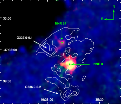
Figure 9.— NuSTAR image of the region around NNR 8. The 3–10 keV band is shown in red, 10–20 keV in green, and 20–40 keV in blue. White contours show the radio continuum emission of the CTB 33 complex from Sarma et al. (1997). Green points denote the positions of NuSTAR sources. G337.0-0.1 is a confirmed supernova remnant while G336.9-0.2 is an HII region. It has been suggested that the magnetar, NNR 24, is associated with this SNR (Brogan et al., 2000). However, the extended emission of NNR 8 is clearly not coincident with G337.0-0.1 and its origin may be an unassociated PWN.

The extended emission of NNR 21 is associated with SNR G337.2+0.1, located at a distance of $\sim 14$ kpc. Using Chandra observations, Jakobsen (2013) found that the radial profile of the SNR exhibits a central compact source, suggesting a pulsar powering a PWN, as well as excess emission at a radius of $\approx 1\farcm 8$, attributable to the SNR shell. The dearth of NuSTAR photons from the central point source does not allow for a significant detection of a pulsar signal, so we cannot confirm the PWN origin of NNR 21. XMM-Newton observations of this SNR revealed that it has a non-thermal spectrum which steepens further from the central core (Combi et al. 2006, hereafter C06), as is seen in many plerionic SNRs (e.g. IC 443, 3C 58, G21.5-0.9; Bocchino & Bykov 2001 and references therein). Spectral fitting of the NuSTAR and Chandra data results in a higher column density ($N_{\mathrm{H}}=2.6^{+0.9}_{-0.7}\times 10^{23}$ cm^-2) and steeper photon index ($\Gamma=2.6^{+0.5}_{-0.4}$) than measured by C06 for the pulsar/PWN (central source and extended emission combined). The Chandra/NuSTAR-derived photon index, while consistent at the 90% confidence level with the XMM measured value ($\Gamma=1.82\pm 0.45$), is steeper than expected for a pulsar/PWN. We find that the unabsorbed 2–10 keV luminosity of NNR 21 is $3\times 10^{34}$ erg s^-1, and thus the $L_{X}-\dot{E}$ correlation from Possenti et al. (2002) yields a spin-down luminosity estimate of $\dot{E}\approx 1.5\times 10^{37}$ erg s^-1. The spin-down luminosity that is estimated using the $\Gamma-\dot{E}$ correlation from Gotthelf (2003) is in good agreement if it is based on the XMM-derived $\Gamma=1.8$ ($\dot{E}\approx 1.4\times 10^{37}$ erg s^-1), but it is at odds if the Chandra/NuSTAR-derived $\Gamma$ is adopted ($\dot{E}>1.7\times 10^{38}$ erg s^-1).

Comparing our power-law fits of NNR 21 with the results of C06, the Chandra/NuSTAR-derived $N_{\mathrm{H}}$ is statistically higher than the $N_{\mathrm{H}}=1.15\pm 0.27\times 10^{23}$ cm^-2 measured by C06 for the whole PWN, but it is consistent at better than 90% confidence with the value C06 measure for the outer region of the PWN ($N_{\mathrm{H}}=1.62\pm 0.56\times 10^{23}$ cm^-2), which excludes the central 12^′′-radius region; this central region has a much lower column density of $5.9\pm 1.5\times 10^{22}$ cm^-2. Even if we compare the results of our apec model fits with C06, the Chandra/NuSTAR-derived $N_{\mathrm{H}}$ is more consistent with the $N_{\mathrm{H}}$ value that C06 measure for the outer region rather than the whole PWN. One possible explanation for these spatial and temporal $N_{\mathrm{H}}$ variations is that the outer region of the PWN is interacting with a molecular cloud. This scenario would naturally explain the higher $N_{\mathrm{H}}$ measured in the outer region of the PWN compared to the central region by C06, and the increase in the average $N_{\mathrm{H}}$ measured for the whole PWN between the 2004 XMM observation and the 2011 Chandra observation could be attributed to a larger fraction of the PWN interacting with the dense interstellar medium as the PWN expands. Additional X-ray observations to obtain spatially resolved spectroscopy of NNR 21 are required to better understand the origin of the spectral variations exhibited by this SNR.

VI.1.3 Magnetars

A known magnetar and a magnetar candidate are present in the NuSTAR Norma survey. NNR 24 is a known soft gamma-ray repeater, SGR 1627-41, which was discovered by the Burst and Transient Source Experiment (BATSE) when the source went into outburst in 1998 June (Woods et al., 1999). It has been suggested that this SGR is associated with the young SNR G337.0-0.1 in the CTB 33 complex (Hurley et al., 1999), shown in Figure 9. SGR 1627-41 last went into outburst in 2008 (Esposito et al., 2008) and it was found to have returned to quiescence by 2011 in NARCS observations (An et al., 2012). The cross-normalization constant from fitting the NuSTAR and Chandra spectra is consistent with 1.0 at 90% confidence, indicating that the magnetar persists in quiescence and has not significantly decreased in flux since 2011. We measure a photon index of $5.0^{+2.2}_{-1.4}$ which is steeper but still consistent with that measured by An et al. (2012) at 90% confidence. Assuming a distance of 11 kpc, based on the association with the CTB 33 complex, we find that NNR 24 has unabsorbed luminosities of $2.3\times 10^{33}$ erg s^-1 in the 3–10 keV band and $5.2\times 10^{31}$ erg s^-1 in the 10–20 keV band.

NNR 10, a transient source, may also be a magnetar. The long-term variability and spectral analysis of this source is described in detail in T14, and our spectral analysis yields consistent results. The flux of NNR 10 varies by more than a factor of 20 over a three-week period, with the peak of activity lasting between 11 hours and 1.5 days and having a soft spectrum with $\Gamma=4.1^{+0.9}_{-0.8}$ or $kT=3^{+2}_{-1}$ keV for a bremsstrahlung model. The high $N_{\mathrm{H}}$ measured from the X-ray spectrum of NNR 10 suggests that this source is located at $\gtrsim 10$ kpc and thus has a peak $L_{X}\gtrsim 10^{34}$ erg s^-1 in the 2–10 keV band. As argued by T14, NNR 10 is most likely either a shorter than average outburst from a magnetar or an unusually bright flare from a chromospherically active binary.

VI.1.4 Black hole binary candidate

Among the remaining NuSTAR Norma sources not discussed in § VI.1.1- VI.1.3, NNR 15 stands out as the only source showing clear short-timescale variability in the NuSTAR band and also having the lowest median energy. As can be seen in Figure 5, NNR 15 displays flaring behavior in the 3–20 keV band; during one flare lasting about 15 ks, the source flux increases by a factor of $>$6, and during a smaller flare lasting about 7 ks, the flux increases by a factor of $>$2. This source also shows variability on year-long timescales since the 3–10 keV flux measured in 2013 NuSTAR observations is a factor of 2 higher than the Chandra flux measured from 2011 observations. The NuSTAR and Chandra spectra are well-fit by an absorbed power-law model with very low $N_{\mathrm{H}}$, indicating that the source must reside within a few kiloparsecs, and $\Gamma=2.6\pm 0.4$ (or $kT=2.9^{+1.0}_{-0.7}$ keV for a bremsstrahlung model). No Fe line is visible in the spectrum, but due to the limited photon statistics, we can only constrain the equivalent width of a potential Fe line feature to be $<1.7$ keV, a loose constraint that does not help to distinguish between different types of X-ray sources. Assuming a distance of 2 kpc, NNR 15 has an average unabsorbed 3–20 keV luminosity of $1.5\times 10^{32}$ erg s^-1. Its optical/infrared counterpart has been identified as a mid-GIII star (Rahoui et al., 2014).

Based on these properties, we identify NNR 15 as a black hole LMXB candidate in quiescence, although an active binary (AB) or CV origin cannot be entirely ruled out. In quiescence, ABs typically have $L_{X}=10^{29-31.5}$ erg s^-1 and $kT<2$ keV (Dempsey et al., 1993) but they can exhibit flares with peak luminosities of $\sim 10^{32}$ erg s^-1 and $kT\approx 10$ keV (Franciosini, Pallavicini & Tagliaferri, 2001). However, AB flares tend to have very short rise times and long decay times (Pandey & Singh, 2012), whereas the flares seen in NNR 15 appear to have more symmetric profiles. CVs have $L_{X}=10^{29-33}$ erg s^-1 and $kT=1-25$ keV (e.g. Eracleous, Halpern & Patterson 1991; Muno et al. 2004), with magnetic CVs being more luminous and spectrally harder than non-magnetic CVs (Barlow et al. 2006; Landi et al. 2009), so their properties are consistent with NNR 15. However, the flaring exhibited by NNR 15 is not typically seen in CVs. Non-magnetic CVs have outbursts that last several days and have recurrence times of weeks to months; intermediate polars (IPs) have outbursts of similar duration but which are very rare (Hellier, Mukai & Beardmore 1997; Szkody et al. 2002), and polars exhibit flares with $\sim$hour-long durations but they tend to be very soft ($kT<1$  keV; Choi, Dotani & Agrawal 1999; Still & Mukai 2001; Traulsen et al. 2010). The properties of NNR 15 are reminiscent of the quiescent state of V404 Cyg, a well-known LMXB hosting a black hole (BH; Makino et al. 1989; Casares, Charles & Naylor 1992; Shahbaz et al. 1996). Recent NuSTAR observations of V404 Cyg in quiescence show that, in the 3–25 keV band, its power-law spectrum has $\Gamma=2.35\pm 0.2$ and it exhibits flux variations of up to a factor of 10 over periods of a few hours (Rana et al., 2016). Given the similarities between the X-ray spectra and light curves of NNR 15 and V404 Cyg, NNR 15 is most likely a BH LMXB, although it may be a CV or an AB. To order-of-magnitude accuracy, it is estimated that $\sim 1000$ quiescent BH LMXBs reside in the Galaxy (Tanaka, 1996); the primary source of uncertainty in this estimate is our limited knowledge of the typical recurrence timescale of BH transients. Making the simplifying assumption that quiescent BH binaries trace the stellar mass distribution of Galaxy and using the estimate of the stellar mass enclosed in the Norma survey area by F14, we would expect $\sim 4$ BH LMXBs to reside in the survey area. Thus, it is at least plausible that one BH binary would be detected in the NuSTAR Norma survey.

VI.1.5 Cataclysmic variables and active galactic nuclei

Based on NARCS results, we expect that the majority of NuSTAR Norma sources should be a mixture of CVs and AGN. CVs typically have thermal spectra with $kT\approx 1-30$ keV although IPs can display even higher temperatures ($kT\approx 30-50$ keV; Landi et al. 2009), while AGN exhibit power-law spectra with $\Gamma\approx 1.5-2$ (Tozzi et al. 2006; Sazonov et al. 2008). The remaining 17 tier 1 sources (NNR 4, 6, 9, 11–13, 16–20, 22, 23, 25–28) have bremsstrahlung temperatures and photon indices consistent with being either CVs or AGN. With the NuSTAR, Chandra, and infrared data available for these sources, there are three primary ways to distinguish CVs and AGN:

• i. If the absorbing column density inferred from X-ray spectral fitting or Chandra quantiles is significantly lower than the integrated interstellar $N_{\mathrm{H}}$ along the line-of-sight to the source, it is a Galactic source.

• ii. If the source does not have a point-like infrared counterpart with $>98$% reliability in the VVV survey, it may be an AGN or a Galactic source with a K or M main-sequence companion, which would fall below the VVV sensitivity limits ($Ks<18$ mag) if located at $\gtrsim 2$ kpc. Since the energy bands used by the Wide-Field Infrared Survey Explorer (WISE; Wright et al. 2010) can be more useful than the $J$, $H$, or $K$ bands for identifying AGN (Stern et al. 2012; Mateos et al. 2012), we also searched for counterparts to the NuSTAR sources in the AllWISE catalog (Cutri & et al., 2013). The BH binary candidate NNR 15 and four tier 2 sources (NNR 29, 30, 31, and 38) have WISE matches located within the 95% positional uncertainty of their Chandra counterparts. The counterparts of NNR 15, 29, and 30 have been idenfitied as low-mass stars through spectroscopic follow-up (Rahoui et al., 2014), and the other WISE counterparts have $W1-W2<0.1$, far below the typical value of $W1-W2\geq 0.8$ for X-ray luminous AGN (Stern et al., 2012); furthermore, the near-IR spectra of the counterparts of NNR 31 and 38 indicate they are Galactic sources (Corral-Santana et al., in prep). Thus, none of the NNR sources with WISE counterparts are AGN, but we cannot rule out the possibility that some AGN are undetected by WISE. For instance, in the NuSTAR serendipitous survey, which has comparable sensitivity limits to the NuSTAR Norma survey, about 25% of NuSTAR sources at Galactic latitudes $|b|>10^{\circ}$, which are likely to be AGN, do not have a WISE counterpart (Lansbury et al., submitted).

• iii. If the source exhibits strong unshifted Fe emission, it is more likely to be a CV than an AGN. Both magnetic and non-magnetic CVs often exhibit Fe emission; in some sources, individual Fe lines at 6.4, 6.7, and 6.97 keV with equivalent widths of 100–200 eV can be seen, while in others, a broad component centered around 6.7 keV with an equivalent width of up to a few keV is seen, likely resulting from the blending of multiple Fe lines due to low energy resolution (e.g. Mukai & Shiokawa 1993; Ezuka & Ishida 1999; Baskill, Wheatley & Osborne 2005; Bernardini et al. 2012; Xu, Wang & Li 2016). Both type I and type II AGN often exhibit red-shifted Fe emission, with the neutral Fe line typically being strongest, except in some highly ionized AGN where the He-like and H-like Fe lines can rival the neutral Fe line in strength; Fe line emission from AGN typically has equivalent widths $<100$ eV, but they can be higher in Compton-thick AGN (Page et al. 2004; Iwasawa et al. 2012; Ricci et al. 2014). The Fe lines in X-ray binaries also tend to have equivalent widths $\lesssim 100$ eV, so the strength of Fe line emission can also help discriminate between CVs and LMXBs (Hirano et al. 1987; Nagase 1989).

Seven of the tier 1 sources (NNR 4, 6, 9, 12, 18, 19, 25) fulfill at least one of the three criteria listed above and are most likely CVs. NNR 4 meets all three criteria and there is strong evidence that it is an IP, a CV in which the white dwarf (WD) magnetic field is strong enough ($B\approx 10^{6-7}$ G) to truncate the accretion disk and channel the accreting material onto the magnetic poles. The X-ray spectrum of NNR 4 shows low absorption ($N_{\mathrm{H}}<4\times 10^{21}$ cm^-2), indicating it is a Galactic source residing at a distance of $\lesssim 2$ kpc. The joint fitting of the Chandra and NuSTAR spectra provides evidence for partial-covering absorption, which is frequently observed in IPs as some of the X-rays produced in the accretion column pass through the accretion curtain on their way to the observer (de Martino et al. 2004; Bernardini et al. 2012). The near-IR counterpart of NNR 4 is variable and displays emission lines often produced in the accretion streams of IPs (Rahoui et al., 2014). Furthermore, this source also exhibits Fe line emission centered at 6.65${}^{+0.10}_{-0.06}$ keV line with high equivalent width ($0.9^{+0.2}_{-0.1}$ keV), and a 7150 second period detected by Chandra, both of which are typical for IPs (Scaringi et al. 2010). NNR 4 exhibits flux variations on month-year timescales, which is more typical for non-magnetic CVs and polars than IPs (Ramsay et al., 2004), but the flux only varies by a factor $<2$, so the case for this source being an IP remains strong. Assuming a distance of 2 kpc, the unabsorbed 3–10 keV luminosity of NNR 4 is $2-4\times 10^{32}$ erg s^-1, which is within the luminosity range of IPs (Muno et al. 2004 and references therein).

Sources NNR 6, 9, and 12 all have strong Fe emission centered between 6.4 and 6.8 keV and equivalent widths of $1.3\pm 0.4$, $0.4\pm 0.2$, and $1.2\pm 0.4$ keV, respectively, strongly indicating that these sources are CVs since both AGN and X-ray binaries tend to have much weaker Fe emission and the Fe emission from AGN is likely to be redshifted. These large equivalent widths are likely due to multiple Fe lines being blended due NuSTAR’s low energy resolution. Both NNR 6 and 9 are best-fit by thermal models with high plasma temperatures ($kT>15$ keV), which are more typical of magnetic rather than non-magnetic CVs (Landi et al. 2009; Xu, Wang & Li 2016). The lack of flux variations for NNR 6 and 9 suggest they are most likely IPs. In addition, NNR 6 has a low-mass (late GIII) stellar counterpart (Rahoui et al., 2014), lending further support to a CV origin for this source. The nature of NNR 12 is less certain, because its softer spectrum ($kT=6^{+3}_{-1}$ keV for an apec model) is typical for both non-magnetic and magnetic CVs. NNR 21 is likely located at a distance $>10$ kpc given its high $N_{\mathrm{H}}$, so its 3–10 keV luminosity is likely $\gtrsim 2\times 10^{33}$ erg s^-1; this high luminosity coupled with the lack of flux variability suggests this source is also probably an IP.

Another likely IP candidate is NNR 13. This source displays one of the hardest spectra of all the NuSTAR Norma sources, having $kT>21$ keV or $\Gamma=1.0\pm 0.5$. Its very hard spectrum and constant flux over long timescales is typical of IPs.

The nature of NNR 18 is discussed in B14; our spectral analysis yields consistent results, finding a high $N_{\mathrm{H}}$ of $1.9^{+0.9}_{-0.6}\times 10^{23}$ cm^-2 and $\Gamma=2.6^{+1.0}_{-0.8}$. Assuming a distance of $>10$ kpc based on the high $N_{\mathrm{H}}$ value, NNR 18 has an unabsorbed 3–10 keV luminosity $\gtrsim 5\times 10^{33}$ erg s^-1. NNR 18 has an early MIII counterpart and exhibited mild X-ray variability on short timescales in Chandra observations. As discussed by B14, these properties are consistent with an IP or an LMXB. Another possibility is that this source is a hard-spectrum symbiotic binary (SB) hosting a WD or a symbiotic X-ray binary (SyXB) hosting a NS (Luna et al., 2013); the compact objects in SBs and SyXBs accrete material from the wind of a red giant companion, which is typically of spectral type M or K (Morihana et al., 2016). Hard-spectrum SBs and SyXBs display X-ray luminosities between $10^{32}$ and $10^{34}$ erg s^-1 (Masetti et al. 2002; Smith et al. 2008; Nespoli, Fabregat & Mennickent 2010), and variability on short and long timescales (Luna & Sokoloski 2007; Corbet et al. 2008). An IP origin is favored for NNR 18 based on its low levels of variability, while its estimated luminosity and the M giant spectral type of its counterpart favors an SB or SyXB origin.

NNR 19 and 25 show low absorption in their X-ray spectra, indicating they are Galactic sources and probably located at a distance of a few kpc. Both sources are transients which were not detected in NARCS, but they are detected in follow-up Chandra observations taken 3 and 34 days after the NuSTAR observations, respectively. The flux of NNR 25 increased by a factor of $\geq 4$ in the couple of years between the NARCS and NuSTAR observations and remained high for at least 34 days. NNR 19 was detected at a consistent flux level in multiple NuSTAR observations that span $\approx$100 days. About 250 days before it is first detected by NuSTAR, the 90% confidence upper limit for its 3–10 keV photon flux is $2\times 10^{-6}$ cm^-2 s^-1 (a factor 4 below its peak flux), and about 40 days after it is detected by NuSTAR, its flux falls below $4\times 10^{-6}$ cm^-2 s^-1. Thus, we find that the flux of NNR 19 increased by a factor of $\geq 4$ and remained high for a period between 100 and 400 days. In addition, NNR 19 was detected in the archival Chandra ObsID 7591, demonstrating that this transient experienced an outburst in 2007, during which its flux was a factor of $\geq 7$ higher than the upper limit measured by NARCS in 2011. The spectra of NNR 19 and 25 have $kT=11^{+18}_{-4}$ keV ($\Gamma=1.7^{+0.3}_{-0.4}$) and $kT>6$ keV ($\Gamma=1.8\pm 0.7$), respectively. The temporal and spectral properties of NNR 19 and 25 most closely resemble those of polars, CVs with magnetic fields so strong ($B>10^{7}$ G) that the white dwarf magnetosphere inhibits the formation of an accretion disk. Thus, compared to other CVs, polar X-ray emission is very sensitive to changes in the mass transfer rate, and they exhibit flux variations of factors $\geq 4$ as they transition between low and high accretion states on $\sim$month-year timescales (Ramsay et al. 2004; Worpel et al. 2016), very similar to the behavior of NNR 19 and 25. No IR counterparts in the VVV survey are found for NNR 19 or 25 within the 90% positional uncertainty determined from Chandra. While the variability and spectra of NNR 19 and 25 would also be consistent with hard-spectrum SBs or SyXBs, the lack of a counterpart with $Ks<18$ mag rules out the possibility that these sources have red giant companions, which should be visible out to $\gtrsim 10$ kpc. In contrast, it is possible for main-sequence K or M-type stars located at distances of a few kiloparsecs to fall below the VVV survey sensitivity.

The nine remaining tier 1 sources (NNR 11, 16, 17, 20, 22, 23, 26, 27, 28) are well-fit either by thermal models with $kT=4-30$ keV or power-law models with $\Gamma\approx 2$, consistent with the spectra of CVs, SBs, SyXBs, LMXBs, or AGN; the uncertainties in the spectral parameters for many of these sources are quite large since they are among the faintest in our survey. All of these sources have high absorption, that is equal to or in excess of the ISM column density through the Galaxy, and they lack IR counterparts, so it is difficult to determine whether they are Galactic or extragalactic. The lack of counterparts does rule out the possibility that these sources are SBs or SyXBs since their red giant companions should be visible through most of the galaxy given the sensitivity of the VVV survey ($Ks<18$ mag). Based on the log$N$-log$S$ distribution of AGN measured in the COSMOS survey (Cappelluti et al., 2009) and accounting for Galactic absorption, conversion from the 2–10 keV to the 3–10 keV band, and the sensitivity curve of the NuSTAR Norma survey (see § VI.2), we estimate that about five AGN are present in this survey. Therefore, roughly half of the remaining tier 1 sources may be AGN. The other half are probably CVs since quiescent LMXBs are expected to be relatively rare (Tanaka, 1996). Additional NuSTAR or XMM observations are required to distinguish between the possible CV or AGN origin of these nine sources by measuring the strength of Fe line emission and better constraining their spectral hardness. The 3–10 keV fluxes of NNR 11, 20, and 28 vary by factors of $>5$ between the NARCS and NuSTAR observations. Such long-term variability is common for AGN, polars, and non-magnetic CVs (Orio, Covington & Ögelman 2001; Markowitz & Edelson 2004; Ramsay et al. 2004; Baskill, Wheatley & Osborne 2005), so it does not help us discriminate betwen Galactic and extragalactic sources but it at least excludes an IP origin for these three sources.

The ten tier 2 sources included in our catalog do not have enough NuSTAR counts to meaningfully constrain their spectral properties, but their distribution in the Chandra quantile diagram is very similar to the distribution of the 17 tier 1 sources described in this subsection; two are foreground sources while the rest are heavily absorbed and have $\Gamma<2$. Seven of these tier 2 sources (NNR 29, 30, 31, 34, 35, 36, and 38) have reliable IR counterparts, three of which (NNR 29, 30, and 36) have been spectrally identified as low-mass stars (Rahoui et al., 2014). These seven sources are likely to be a mixture of CVs, SBs, and SyXBs like the majority of identified tier 1 sources. Sources NNR 29 and 36 display such low absorption that they are likely located within a few kpc and thus have 3–10 keV luminosities $\lesssim 3\times 10^{31}$ erg s^-1, so they could also be active binaries given their low luminosity (Strassmeier et al., 1993). An AGN origin cannot be ruled out for NNR 34 and 35, which have VVV counterparts but are not detected by WISE. NNR 32, 33, and 37 lack IR counterparts and are heavily absorbed, and could be AGN or Galactic sources. Based on the log$N$-log$S$ derived for AGN and CVs in the Norma region by F14, a 1:2 ratio of AGN to CVs/ABs is expected in the 2–10 keV flux range of these tier 2 sources (4$\times 10^{-14}<f_{X}<1\times 10^{-13}$ erg cm^-2 s^-1). Such a ratio is plausible among tier 2 sources given the current constraints we can place on their physical nature. However, it is odd that none of the sources which may be AGN are detected by WISE with $W1-W2\geq 0.8$, since the majority of AGN discovered in the NuSTAR serendipitous survey have these properties (Lansbury et al., 2016). The fact that our AGN candidates either lack IR counterparts or have only VVV, but not WISE, counterparts indicates that, if they truly are AGN, they are likely to have low-luminosities ($L_{X}\lesssim 10^{43}$ erg s^-1).

VI.1.6 On the search for low-luminosity high-mass X-ray binaries

As discussed in §I, one of reasons the Norma arm was targeted by Chandra and NuSTAR was to search for low-luminosity HMXBs with fluxes below the sensitivity limits of previous surveys. A key criterion for identifying an HMXB candidate is to find a source with a high-mass stellar counterpart, which should be visible in the infrared through the whole Galaxy in the VVV survey. Of the Norma sources detected by NuSTAR, only two, NNR 7 and 14, have high-mass stellar counterparts and their broadband X-ray spectra indicate they are CWBs (see §VI.1.1). However, there are three Chandra sources, NARCS 239, 1168, and 1326, with high-mass stellar counterparts (Rahoui et al., 2014) which were not detected by the NuSTAR Norma survey. The $2-10$ keV Chandra fluxes of these sources ($f_{X}\approx 7-8\times 10^{-14}$ erg cm^-2 s^-1; F14) are comparable to the sensitivity limit of the NuSTAR survey (see §VI.2), and thus it is not surprising that they are not detected. In the Chandra band, these three sources have harder spectra than NNR 7 and 14, residing in a region of quantile space consistent with $\Gamma\approx 2$ power-law spectra (F14), which are typical of accreting HMXBs.

Future spectroscopic observations of the infrared counterparts of these Chandra sources will confirm whether these systems are HMXBs and help to estimate better distances to these sources. Once we determine how many of these HMXB candidates, if any, are truly HMXBs, the constraints provided by the Norma surveys on the faint end of the HMXB luminosity function will be presented in a future paper. By extrapolating the measured slope of the HMXB luminosity function above $10^{34}$ erg s^-1 to lower luminosities, F14 predicted that at least a few HMXBs should be detected in the Norma region with $f_{X}>7\times 10^{-14}$ erg cm^-2 s^-1. Thus, if the three HMXB candidates are confirmed, the number of HMXBs in the Norma region would be consistent with a continuation of the HMXB luminosity function slope to lower luminosities, but if none of these sources prove to be HMXBs, it would imply that the HMXB luminosity function flattens substantially at $L_{X}<10^{34}$ erg s^-1.

VI.2. Survey sensitivity

To compute the sky coverage for the NuSTAR Norma survey, we used the same method employed for NARCS, which is taken from Georgakakis et al. (2008). For a given detection probability threshold, $P_{\mathrm{thresh}}$, we determined the minimum number of total counts required for a detection ($C_{\mathrm{lim}}$) at each position in the image, such that $P(\geq C_{\mathrm{lim}})$ = $P_{\mathrm{thresh}}$. To this end, we made background maps in the 3–10 keV and 10–20 keV bands by removing the counts within 60^′′ (90^′′) radius circular regions centered on the point (extended) source positions listed in Table LABEL:tab:srclist, and then filling in these regions by randomly distributing the expected background counts determined from the local background. Using these background maps, we calculated the mean expected background counts ($\langle C_{\mathrm{bkg}}\rangle$) in circular regions centered on each pixel with radii equal to the 15, 22, and 30% PSF enclosures, which are the cell sizes we used for source detection (see § IV). The probability that the observed counts will exceed $C_{\mathrm{lim}}$ within a particular region is

$$P(\geq C_{\mathrm{lim}})=\gamma(C_{\mathrm{lim}},\langle C_{\mathrm{bkg}}\rangle)$$ (2)

where $\gamma(a,x)$ is the lower incomplete gamma function, defined as

$$\gamma(a,x)=\frac{1}{\Gamma(a)}\int_{0}^{x}e^{-t}t^{a-1}dt$$ (3)

Calculating $C_{\mathrm{lim}}$ requires setting $P(\geq C_{\mathrm{lim}})=P_{\mathrm{thresh}}$, and inverting Equation 2 numerically.

Then we computed the probability of detecting a source of a given flux $f_{X}$ at each pixel, given by

$$P_{f_{X}}(\geq C_{\mathrm{lim}})=\gamma(C_{\mathrm{lim}},C_{\mathrm{src}})$$ (4)

and $C_{\mathrm{src}}=f_{X}t_{\mathrm{exp}}A_{\mathrm{src}}\epsilon+\langle C_{\mathrm{bkg}}\rangle$, where $t_{\mathrm{exp}}$, $A_{\mathrm{src}}$, and $\epsilon$ are the exposure time, mean effective area, and unabsorbed energy flux to observed photon flux conversion factor, respectively. For $\epsilon$, we used the mean ratio of photon flux to energy flux measured for tier 1 sources in a given energy band. To estimate the effective area at each pixel location, we made vignetting-corrected exposure maps, and by comparing the ratio of the vignetting-corrected exposure over the uncorrected exposures to the effective areas of tier 1 sources, we derived a linear relation to convert the exposure ratio at a given location to the effective area for the average source spectrum. These relations were derived using vignetting corrections evaluated at 8 keV for the 3–10 keV band and at 10 keV for the 10–20 keV band; they were also calibrated for the three different cell sizes.

There are a few possible sources of systematic error in our calculation of the sky coverage curves. Different $\epsilon$ values and effective area to exposure ratio relations were derived based on non-parametric and modeling-derived fluxes to account for systematic errors associated with flux calculation methods; the sky coverage curves derived using these different fluxes vary by about 0.1 dex. Another potential source of systematic error arises from our use of the average source spectrum as representative for the NuSTAR Norma sources; based on the spread of spectral properties they exhibit, a systematic error of roughly 0.1 dex on the sky coverage could result from the choice of a representative source spectrum. Finally, the calculated sky coverage includes all the observations shown in Figures 1 and 2, but, as can be seen, a significant wedge of stray light and some residual ghost rays are present, especially in the 3–10 keV band. This contamination effectively reduces our sky coverage, because even though there were about 20 clusters of pixels in these regions which exceeded our detection threshold, we ascribed most of them to artifacts associated with stray light and ghost rays rather than true sources; the only exceptions which we included in our final source list (NNR 2, 6, 10, 16, 18) were either very bright sources, had bright ($\gtrsim 10^{-5}$ photons cm^-2 s^-1) Chandra counterparts, or had a clear point-like morphology. Since the contaminated areas only make up about 2% of the total survey area, their inclusion in our sky coverage does not significantly impact our log$N$-log$S$ results.

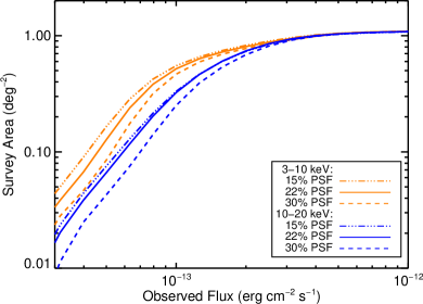
Figure 10.— Sky coverage of the NuSTAR Norma Region survey for different energy bands and PSF enclosure fractions. The curves in this plot use a photon flux to energy flux conversion factor based the spectral modeling of tier 1 sources.

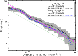
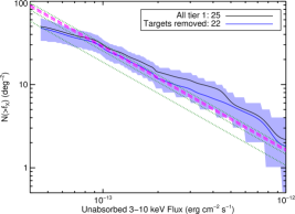
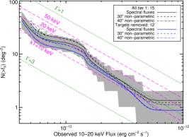
Figure 11.— All: The log$N$-log$S$ distributions shown in black include all tier 1 sources exceeding the detection threshold in a given energy band; the gray band shows the 1$\sigma$ errors on the log$N$-log$S$ distribution. The log$N$-log$S$ distributions shown in blue exclude NNR 2, 4, and 5, which were specifically targeted by NuSTAR. The green dotted (magenta dashed) lines show the NARCS log$N$-log$S$ converted from unabsorbed 2–10 keV into the given bands assuming power-law spectral models with $\Gamma=3$, 2, and 1 (thermal models with $kT$=10, 20 and 50 keV). When converting the NARCS distribution into the observed 3–10 or 10–20 keV bands, a column density of $N_{\mathrm{H}}=10^{23}$ cm^-2 is used, the mean of measured $N_{\mathrm{H}}$ values for the NuSTAR sources; varying $N_{\mathrm{H}}$ between $0.7-2.0\times 10^{23}$ cm^-2 does not significantly change the conversion factor. Top left: The log$N$-log$S$ distribution in the 3–10 keV band, calculated using observed fluxes derived from spectral fitting, as well as non-parametric fluxes calculated from aperture photometry using 30^′′ and 40^′′ radius regions. Top right: The log$N$-log$S$ distribution in the 3–10 keV band calculated using unabsorbed fluxes derived from spectral fitting. The blue band shows the $1\sigma$ errors on the distribution shown in blue. Bottom: Same as top except the log$N$-log$S$ distributions are shown as a function of observed 10–20 keV flux.

The sky coverage was calculated as the sum of probabilities in Equation 4 over all pixels multiplied by the solid angle per pixel. We repeated this calculation for a range of fluxes to produce a sensitivity curve for each of the three detection cell sizes in both the 3–10 keV and 10–20 keV bands. Figure 10 shows the sky coverage for different energy bands and cell sizes. We used the sensitivity curves for the 22% PSF enclosures to calculate the log$N$-log$S$ distribution and sensitivity limits of our survey in the 3–10 keV and 10–20 keV bands, because all but one of the 26 (17) tier 1 sources which were detected in the 3–10 keV (10–20 keV) band were detected in the 22% PSF trial maps, and the 22% PSF sky coverage represents a rough average of the different PSF fraction curves. The deep field of the NuSTAR Norma survey has an area of about 0.04 deg² and sensitivity limits of $4\times 10^{-14}$ erg cm^-2 s^-1 ($5\times 10^{-14}$ erg cm^-2 s^-1) in the observed (unabsorbed) 3–10 keV band and $4\times 10^{-14}$ erg cm^-2 s^-1 in the 10–20 keV band. The shallow survey has an area of $\sim$1 deg² with sensitivity limits of $1\times 10^{-13}$ erg cm^-2 s^-1 ($1.5\times 10^{-13}$ erg cm^-2 s^-1) in the observed (unabsorbed) 3–10 keV band and $1.5\times 10^{-13}$ erg cm^-2 s^-1 in the 10–20 keV band.

VI.3. Log$N$-log$S$ distribution

Since many of the NuSTAR Norma sources have fluxes approaching our sensitivity limits, when calculating the number-count distribution for our survey, it is important to consider the effect of Poisson fluctuations of the source and background counts on the measured source flux. Thus, rather than assigning a single flux value to each source, we determine its flux probability distribution by computing the source count distribution from Equation A21 in Weisskopf et al. (2007) and converting counts to energy fluxes. The number count distribution is then equal to the sum of the flux probability distributions of individual sources, divided by the sensitivity curve calculated in § VI.2.

We compute log$N$-log$S$ distributions in the 3–10 keV and 10–20 keV bands, both for observed and unabsorbed fluxes; in order to check for systematic errors, we perform these calculations using both the modeling-derived and non-parametric fluxes. When constructing the distribution in a given energy band, we only included the sources that exceed the detection threshold in that particular energy band. In addition, in order to compare the NuSTAR number-count distribution with that derived from NARCS, we excluded extended sources, and for sources that are blended in NuSTAR observations but resolved with Chandra, we estimate the NuSTAR fluxes of individual sources by assuming the ratio of fluxes (see comments in Table LABEL:tab:spectra) of the two sources is the same in NuSTAR as it is in the Chandra 2–10 keV band. Thus, NNR 8 is excluded from the sample of sources used in the number-count distribution, the fluxes of the point sources at the center of the extended sources, NNR 3 and 21, are estimated to be 30% and 20% of the total respectively, and the fraction of NNR 7’s flux attributed to NARCS 1278 and 1279 is 30% and 70%, respectively.

We calculated the statistical errors of the log$N$-log$S$ distribution using the bootstrapping method. We account for the errors associated with our sample size as well as the distribution of fluxes within that sample by generating new samples of sources from our original list used to calculate the log$N$-log$S$ distribution. For each new sample, we draw the sample size ($N_{\mathrm{sample}}$) from a Poisson distribution with mean equal to the original sample size, and then randomly select $N_{\mathrm{sample}}$ sources from the original list. We generate 10,000 new samples and calculate the resulting log$N$-log$S$ distribution for each of them. Then we use the simulated distributions to determine the 1$\sigma$ upper and lower confidence bounds of the measured log$N$-log$S$ distribution. The 1$\sigma$ statistical errors are comparable in size to the systematic errors associated with the sensitivity curves, which are discussed in §VI.2.

In addition to the possible sources of systematic error already discussed, there is a simplification in our log$N$-log$S$ calculation which could bias our measurements. As described in §IV.2, we require that a source exceed the detection threshold in two or three trial maps in order to be included in our source list, but our log$N$-log$S$ calculation does not explicitly account for this criterion. This criterion helps to screen out spurious detections which may occur in a given trial map but are unlikely to correlate across different energy bands or aperture sizes; however, it is an easy criterion for a real source to pass, since it is very likely for a real source exceeding the threshold in one trial map to exceed it in at least another trial map with the same energy band but a different PSF enclosure fraction. Thus, we do not expect our detection criterion to substantially alter the sensitivity curves or, in turn, the log$N$-log$S$ distribution. To gauge the magnitude of the possible bias due to our choice of sensitivity curve, we produced different versions of the log$N$-log$S$ distribution in the 3–10 keV and 10–20 keV bands, adopting sensitivity curves for different PSF enclosures, and testing the effect of limiting the source subsample to tier 1 sources exceeding the threshold in the trial map with both the same energy band and PSF enclosure as the sensitivity curve rather than just the same energy band. The resulting variations in our log$N$-log$S$ results are smaller than the statistical uncertainties.

Figure 11 shows the resulting log$N$-log$S$ distributions for the NuSTAR Norma region. In these panels, magenta and green lines show the log$N$-log$S$ distribution measured by NARCS converted from the unabsorbed 2–10 keV band to the NuSTAR bands assuming different spectral models, thermal models with $kT=10$, 20, and 50 keV and power-law models with $\Gamma=1$, 2, and 3; when converting to observed energy fluxes, a typical $N_{\mathrm{H}}$ value of 10²³ cm^-2 is used. The log$N$-log$S$ distributions shown in black include all tier 1 sources that exceed the detection threshold in a given energy band, while the blue distributions exclude the sources that were specifically targeted by NuSTAR and detected (NNR 2, 4, and 5), which could unnaturally inflate the log$N$-log$S$ distribution. As shown in the top panel, there is little difference between the NARCS distributions converted using different spectral models into the observed 3–10 keV band, which is not surprising given its large amount of overlap with the Chandra 2–10 keV band. Regardless of how the source energy fluxes are calculated, the NuSTAR distribution is consistent with the NARCS distribution at 1$\sigma$ confidence, exhibiting a similar slope of $\alpha\approx-1.24$. The NuSTAR distribution only deviates significantly from the NARCS distribution at low fluxes. This discrepancy may be due to the Eddington bias or variance in the spatial density of sources, given that the sources with the lowest fluxes are only detected in the deep HESS field, which is only 100 arcmin² in size.

The middle panel of Figure 11 shows the log$N$-log$S$ distribution calculated using the unabsorbed 3–10 keV fluxes from spectral fitting. Although this distribution is still largely consistent with the NARCS distribution at 1$\sigma$ confidence when the sources specifically targeted by NuSTAR are removed (shown in blue), the NuSTAR distribution is slightly higher than the Chandra distribution above $>3\times 10^{-13}$ erg cm^-2 s^-1. The fact that this excess is only seen using unabsorbed 3–10 keV fluxes but not the observed 3–10 keV fluxes suggests that, for some sources, we measure $N_{\mathrm{H}}$ values that are too high and thus overcorrect for absorption.

The bottom panel of Figure 11 shows the log$N$-log$S$ distributions calculated using modeling-derived and non-parametric fluxes in the observed 10–20 keV band. Since there is very little difference between the observed and unabsorbed 10–20 keV fluxes, the log$N$-log$S$ distribution in the unabsorbed 10–20 keV band is not shown. Although the 10–20 keV NuSTAR distributions deviate from a simple power-law due to the small number of sources (16) detected in this hard X-ray band, overall the slope is still consistent with the NARCS slope. The normalizations of the different NARCS distributions extrapolated into the 10–20 keV band are distinct depending on the spectral model assumed; for the NuSTAR and NARCS normalizations to be consistent, the average spectrum of Norma sources must either have $kT=10-20$ keV or $\Gamma=2$. This average spectrum is indeed consistent with the individual spectral fits of most of the NuSTAR sources and their locations in the NuSTAR quantile space.

VI.4. Comparison to the Galactic Center NuSTAR population

Comparing the log$N$-log$S$ distributions of sources in the Norma region and the 1${}^{\circ}\times 0.6^{\circ}$ Galactic Center (GC) region surveyed by NuSTAR, the number density of NuSTAR sources is $\approx 2$ times higher in the GC (Hong et al., 2016), which is to be expected since the stellar density in the vicinity of the GC is higher than the stellar density along the line-of-sight of the Norma region. The power-law slope of the number-count distribution is also steeper in the GC ($\alpha\approx-1.4$; Hong et al. 2016), which is consistent with the trend that is seen for Chandra sources in the GC and the field in the 0.5–8 keV band (Muno et al., 2009). In order for the normalizations of the GC NuSTAR and Chandra number-count distributions to be consistent, the typical spectrum of GC sources must either have $kT=20-50$ keV or $\Gamma\approx 1.5$, which is harder than the typical spectrum of Norma sources.

Hong et al. (2016) argue that $40-60$% of NuSTAR GC sources are magnetic CVs, primarily IPs, given their very hard X-ray spectra ($\Gamma\lesssim 1.5$) and the presence of strong Fe emission. All but two of the Norma CV candidates have softer spectra ($\Gamma>1.5$, $kT\lesssim 20$  eV). The spectral differences between the NuSTAR populations in the Norma and GC regions are mirrored in the differences between the Galactic Ridge X-ray emission (GRXE; Revnivtsev et al. 2006a; Revnivtsev, Molkov & Sazonov 2006b; Revnivtsev et al. 2009) and the central hard X-ray emission (CHXE) discovered by NuSTAR in the GC (Perez et al., 2015). The lower temperatures of the Norma CV candidates are consistent with the thermal spectra of the GRXE, whose hot component has a temperature of $kT\approx 15$ keV (Türler et al. 2010; Yuasa, Makishima & Nakazawa 2012), while the high temperatures of GC CVs resemble the $kT>25$ keV emission observed in the inner few parsecs of the Galaxy (Perez et al. 2015; Hong et al. 2016).

However, it is unclear why the X-ray populations in the GC and the disk are different. Under the assumption that most of the sources contributing to the CHXE and GRXE are IPs, the differences in their typical X-ray temperatures have been attributed to differences in their WD masses, with WDs in the GC CVs having masses $\gtrsim 0.8M_{\odot}$ (Perez et al. 2015; Hong et al. 2016) and those in the disk CVs having masses $\approx 0.6M_{\odot}$ (Krivonos et al. 2007; Türler et al. 2010; Yuasa, Makishima & Nakazawa 2012). However, the mean WD mass among all CVs has been measured to be $0.83\pm 0.23M_{\odot}$ (Zorotovic, Schreiber & Gänsicke, 2011), and the X-ray inferred masses of confirmed field IPs are consistent with this higher value of $\approx 0.8M_{\odot}$ (Hailey et al., 2016). The discrepancy between the measured WD masses for field CVs and the lower masses inferred from the temperature of the GRXE suggests that it may be incorrect to assume that the GRXE is dominated by IPs (Hailey et al., 2016). Thus, it may be similarly incorrect to attribute the temperature differences between the NuSTAR CV candidates in the GC and Norma regions to differences in their WD masses.

In fact, as discussed in § VI.1.5, a significant fraction of the Norma CV candidates may not be IPs but rather a mixture of polars, non-magnetic CVs, hard-spectrum SBs, and SyXBs. These types of sources have softer spectra than IPs, and thus the difference in the average temperatures of Norma and GC sources may be explained by variations in the relative fractions of different types of CVs and symbiotic binaries. It is unclear what physical processes would drive variations in the relative fractions of different types of compact object binaries in these two Galactic regions, but investigating these issues further will first require confirmining the true nature of the CV candidates.

The clearest ways of distinguishing different types of CVs and SBs is by measuring the relative flux ratios of their Fe emission lines (Xu, Wang & Li, 2016) or measuring both their spin and orbital periods (Scaringi et al., 2010), but since most of the Norma CV candidates are quite faint, it will be difficult to obtain X-ray spectra or light curves with enough photons to make such measurements with current telescopes. Monitoring the long-term X-ray and infrared variability of the CV candidates, and determining the spectral types of their counterparts more accurately to estimate distances and luminosities will help to identify the nature of these sources.

VII. Conclusions

• 1. We have detected 28 hard X-ray sources in a square-degree region in the direction of the Norma spiral arm surveyed by NuSTAR, which are designated as tier 1 sources. Twenty-three of these sources were previously detected in observations of the Norma Arm Region Chandra survey, one was a well-studied black hole transient (4U 1630-472), and four were newly discovered transients that we followed up and localized with Chandra. Out of 28 sources, 16 of them are detected above 10 keV. In addition, we found ten NARCS sources with 2–10 keV fluxes $>6\times 10^{-6}$ cm^-2 s^-1 that did not exceed our formal detection threshold for NuSTAR but which displayed significant X-ray emission (S/N$>3$) in at least one of three energy bands, which are designated as tier 2 sources. We have provided photometric information for these sources in our catalog but do not include them in our calculation of the log$N$-log$S$ distribution since they do not meet our detection thresholds.

• 2. The log$N$-log$S$ distribution of NuSTAR sources in the 3–10 keV band is consistent with the distribution of 2–1  keV Chandra sources in the Norma region.

• 3. The NuSTAR log$N$-log$S$ distribution in the 10–20 keV band is consistent with the 2–10 keV Chandra distribution if the average spectrum of the NuSTAR sources can be described by a power-law model with $\Gamma=2$ or a single temperature apec model with a plasma temperature between 10 and 20 keV. The broadband (3–40 keV) energy quantiles of the NuSTAR sources show that the majority of sources have photon indices of $\Gamma=2-3$ for a power-law model or $kT=5-30$ keV for a bremsstrahlung model, which are consistent with the spectral parameters required for good agreement between the 10–20 keV and 2–10 keV log$N$-log$S$ distributions.

• 4. We fit the joint Chandra and NuSTAR spectra of all sources with $>100$ counts in the 3–40 keV band, but find that $>300$ NuSTAR counts are required to provide meaningful constraints on spectral model parameters. We find good agreement between the spectral parameters from our fits and the location of sources in the quantile diagrams.

• 5. Four of the sources detected in the NuSTAR Norma Arm Region survey are previously well-studied sources: NNR 1 is the black hole LMXB 4U 1630-472, NNR 2 is the supergiant HMXB IGR J16393-4643, NNR 3 is the PWN and luminous TeV source HESS J1640-465, and NNR 24 is the magnetar SGR J1627-41. Based on the X-ray variability, spectral fits, and infrared counterpart information for each source, we determined the most likely nature of the fainter sources in our survey, which are summarized in Table 11. Sources NNR 5, 8, and 21 are PWN candidates, NNR 7 and 14 are likely colliding wind binaries, NNR 10 is a possible magnetar, and NNR 15 is a quiescent black hole LMXB candidate. The other sources are primarily CV candidates, a mixture of IPs, polars, non-magnetic CVs, and symbiotic binaries. We estimate that five background AGN are present among the tier 1 NuSTAR sources.

• 6. Compared to the NuSTAR sources that are detected in the Galactic Center region, the sources in the Norma region have softer spectra on average. Even restricting the comparison to the CV candidates in these two regions, the Norma CVs exhibit lower plasma temperatures than those in the GC. The $kT\approx 15$ keV temperatures of Norma CV candidates resemble the hot component of the GRXE spectrum.

• 7. If most of the Norma CV candidates are IPs, then their plasma temperatures indicate the white dwarfs in these systems have masses of $\approx 0.6M_{\odot}$, which are lower than the WD masses of $\gtrsim 0.8M_{\odot}$ estimated for the GC IPs. However, we argue that it is more likely that the fraction of IPs relative to polars, non-magnetic CVs, and symbiotic binaries is lower among Norma CV candidates than in the GC region. Since IPs have the hardest X-ray spectra of all these types of sources, a lower fraction of IPs in the Norma region would result in lower plasma temperatures for the average source.

• 8. In order to understand the nature of the hard X-ray sources in the Norma region and why they differ from the hard X-ray sources in the GC region, it is necessary to continue monitoring the X-ray variability of the Norma CV candidates, better characterize the variability and spectral types of their infrared counterparts, and obtain higher quality spectra, especially at Fe line energies, for the brighter sources. Follow-up multiwavelength observations of the candidate PWN, CWBs, and quiescent black hole binary would be useful in furthering our understanding of compact stellar remnants and the evolution of massive stars.

In this appendix, we present the Chandra and NuSTAR spectra of sources NNR 10–27 and residuals for the best-fitting spectral models listed in Table LABEL:tab:spectra. Our spectral analysis is described in § V.7. The spectra of NNR 1, 2, and 3 are shown in King et al. 2014, B16, and G14, respectively, while the spectra of sources NNR 4–9 are shown in Figure 8. In the figures below, Chandra data is shown in black, NuSTAR FPMA data is shown in red, and FPMB data is shown in blue. For NNR 19, black points show the Chandra spectrum from ObsID 7591 while orange points shows the Chandra spectrum from ObsID 16170. For NNR 21, black points denote the Chandra spectrum for the point source and extended emission combined while orange points display the point source contribution alone.

Table 1NuSTAR Observations of the Norma Arm Region

ObsID	Pointing (J2000)			Start Time	Exposure	SL Removal	SL	Other
	R.A. (∘)	Dec. (∘)	PA (∘)	(UT)	(ks)	(FPM)	Source	Contamination
(1)	(2)	(3)	(4)	(5)	(6)	(7)	(8)	(9)
Wide Shallow Survey
First mini-survey
40014001001	248.4829	-47.7204	160.1494	2013-02-24 01:46	18.4			Ghost rays from 4Ub in AB
40014002001	248.3623	-47.6444	160.1471	2013-02-24 11:31	19.5			Ghost rays from 4Ub in AB
40014003001	248.2407	-47.5669	160.1266	2013-02-21 20:31	20.8			Ghost rays from 4Ub in AB
40014004001	248.5977	-47.6374	160.1231	2013-02-22 07:46	19.5			Ghost rays from 4Ub in AB
40014005001	248.4775	-47.5622	160.1304	2013-02-22 17:31	21.3			Ghost rays from 4Ub in AB
40014006001	248.3529	-47.4868	160.1393	2013-02-23 04:46	18.9			Ghost rays from 4Ub in AB
40014007001	248.7099	-47.5554	160.1350	2013-02-23 14:31	22.7			Ghost rays from 4Ub in AB
40014008002	248.5845	-47.4826	160.1196	2013-02-20 23:32	16.6			Ghost rays from 4Ub in AB
40014009001	248.4670	-47.4038	160.1198	2013-02-21 10:46	14.7			Ghost rays from 4Ub in AB
Later observations
40014011002	250.0712	-46.4909	280.7063	2013-06-20 00:06	21.5	AB	4Ua
40014012001	250.0006	-46.4546	280.7266	2013-06-20 14:21	19.7	AB	4Ua
40014013001	249.9200	-46.4004	281.4251	2013-06-21 03:16	20.5	A	4Ua
40014014001	250.2358	-46.3989	285.7049	2013-06-21 17:46	16.4			1.5′ streak in AB
40014015001	250.0770	-46.3706	285.7091	2013-06-22 08:21	19.2
40014016001	250.2620	-46.5441	285.6937	2013-06-23 21:21	19.6	AB	4Ua
40014017001	250.1762	-46.5238	285.6774	2013-06-23 11:51	24.2	AB	4Ua
40014018001	249.9326	-46.3469	286.8740	2013-06-24 00:51	23.8
40014019001	250.1520	-46.3873	286.8743	2013-06-24 15:21	25.6
40014021002	249.1106	-47.1553	168.0928	2014-03-09 21:56	29.1	AB	GX, 4Ua
40014022001	249.0348	-46.9577	168.0985	2014-03-10 15:31	28.4	AB	GX, 4Ua
40014023001	249.2029	-47.1072	168.1000	2014-03-11 07:41	28.8	AB	GX, 4Ua
40014024001	248.8388	-46.9903	168.1169	2014-03-11 23:46	28.1	AB	GX, 4Ua
40014025001	248.8796	-47.0734	168.1144	2014-03-12 17:36	29.1	AB	GX, 4Ua
40014026001	249.1206	-46.9073	168.0941	2014-03-13 11:26	30.2	AB	GX, 4Ua
40014027001	249.1610	-47.0090	168.1171	2014-03-14 03:31	30.2	AB	GX, 4Ua
40014028002	249.0277	-47.1640	168.1544	2014-03-18 12:36	29.6	AB	GX, 4Ua
40014029001	249.9367	-46.8984	168.2590	2014-03-19 04:41	29.2	AB	GX, 4Ua
40014030001	250.2174	-46.7179	168.3050	2014-03-19 20:46	27.3	B	4Ua
40014031001	250.5222	-46.7773	168.3521	2014-03-20 13:01	30.0	B	4Ua
40014032001	250.4317	-46.7896	168.4181	2014-03-21 05:01	30.9	B	4Ua
40014033002	250.4849	-46.6649	168.2038	2014-03-24 10:41	31.5	B	4Ua
40014034001	250.2701	-46.8265	168.1849	2014-03-25 02:46	31.2	AB	GX, 4Ua
40014035001	250.0454	-46.8714	168.1523	2014-03-25 18:56	39.2	AB	GX, 4Ua
30001008002	249.8301	-46.6567	295.0558	2014-06-26 02:21	50.4
30001012002	248.6712	-47.6364	171.9830	2013-03-23 08:31	16.3	A	GX	Ghost rays from 4Ub in AB
30001016002	248.5333	-47.3795	164.6452	2014-03-06 22:56	21.3	AB	GX, 4Ua
30001017002	248.8967	-47.3836	210.3881	2014-05-12 21:31	49.0	AB	GX, 4Ua
30001033002	249.4897	-46.9015	145.8254	2015-01-28 05:16	51.8	AB	GX, 4Ua
30160001002	249.3137	-47.5723	267.7851	2015-06-11 14:46	49.4	AB	GX, 4Ua
30160002002	248.9436	-47.5918	261.9558	2015-06-07 23:46	97.1	AB	GX, 4Ua
30160003002	249.0412	-47.8404	244.4634	2015-05-31 11:11	76.7	AB	GX, 4Ua
40001022002	249.5341	-47.2183	164.5577	2014-03-07 11:51	100.6	AB	GX, 4Ua
Deep HESS Field
30002021002	250.1049	-46.5763	353.7407	2013-09-29 6:56	62.8	AB	GX, 4Ua	SL of unknown origin in A
30002021003	250.1324	-46.5412	353.7551	2013-09-30 16:31	20.8	A	4Ua	SL of unknown origin in A
30002021005	250.2036	-46.5095	161.2653	2014-02-38 23:16	99.5	AB	4Ua
30002021007	250.2027	-46.5145	161.2702	2014-03-06 01:51	35.9	AB	4Ua
30002021009	250.2175	-46.5088	166.7254	2014-03-14 21:21	32.5	AB	4Ua
30002021011	250.2296	-46.5012	179.7925	2014-04-11 13:11	22.5	AB	4Ua
30002021013	250.1923	-46.5268	227.3736	2014-05-25 01:56	21.6
30002021015	250.1802	-46.5601	289.9801	2014-06-23 12:51	29.2	A	4Ua
30002021017	250.1814	-46.5644	295.1336	2014-06-25 13:31	22.0
30002021019	250.1913	-46.5447	295.1661	2014-06-28 01:20	19.5
30002021021	250.1762	-46.5687	295.1179	2014-06-30 01:41	19.8
30002021023	250.1892	-46.5586	311.5738	2014-07-11 02:21	22.1
30002021025	250.1569	-46.5398	330.9082	2014-08-10 05:36	21.9	A	IGR, 4Ua	6′ streak in B
30002021027	250.1477	-46.5524	344.3607	2014-09-11 10:56	20.0	AB	GX, 4Ua
30002021029	250.1247	-46.5392	356.5397	2014-10-11 01:01	22.1	AB	4Ua
30002021031	250.1400	-46.5260	15.7729	2014-11-05 07:56	4.3	AB	4Ua
30002021033	250.2058	-46.4950	129.7677	2015-01-08 04:46	4.2
30002021034	250.2115	-46.4858	129.7237	2015-01-12 18:16	16.7
30002031036	250.2188	-46.5018	154.4146	2015-02-16 02:41	31.8	AB	4Ua, 4Ub
Notes: (4) Position angle (east of North). (7) Focal plane module(s) from which stray light background photons from sources in column 8 were removed. (8) Stray light background sources: GX = GX 340+0, 4Ua = 4U 1624-49, 4Ub = 1630-472, IGR = IGR J16318-4848. Although additional stray light from IGR J16320-4751 was present in some of the first mini-survey observations, and stray light from 4U 1624-49 and GX 340+0 was present in observation 30001008002, this stray light background was not removed since real sources could be seen in the raw data residing in the stray light-contaminated regions. The contamination in observations 30002021002A, 30002021003A, 30002021036B, and 30001012002 was so extensive that these observations were not included in our analysis.

Table 2Archival Chandra observations used in this study

Chandra	Pointing (J2000)		Start Time	Exposure	References
ObsID	R.A. (∘)	Dec. (∘)	(UT)	(ks)
(1)	(2)	(3)	(4)	(5)	(6)
7591	250.187126	-46.520108	2007-05-11 11:01	28.8	Lemiere et al. 2009
11008	250.134287	-46.393394	2010-06-19 22:10	39.6	Rahoui et al. 2014
Norma Arm Region Chandra Survey (NARCS)					Fornasini et al. 2014
12507	250.373201	-46.662951	2011-06-06 10:15	18.8
12508	250.155011	-46.530604	2011-06-06 15:57	18.5
12509	249.937805	-46.397816	2011-06-06 21:22	19.4
12510	250.180190	-46.812896	2011-06-09 12:29	19.9
12511	249.961646	-46.681456	2011-06-17 11:15	19.3
12512	249.743370	-46.550407	2011-06-27 04:52	20.5
12513	249.984947	-46.965904	2011-06-27 11:00	20.2
12514	249.767582	-46.829470	2011-06-10 16:07	19.8
12515	249.550110	-46.695978	2011-06-10 22:04	19.5
12516	249.790838	-47.111874	2011-06-11 03:46	19.5
12517	249.572205	-46.978413	2011-06-11 09:28	19.5
12518	249.354673	-46.844540	2011-06-11 15:10	19.5
12519	249.594334	-47.262081	2011-06-13 04:25	19.3
12520	249.375577	-47.128273	2011-06-13 10:13	19.0
12521	249.157932	-46.994022	2011-06-13 15:46	19.0
12522	249.396933	-47.410725	2011-06-13 21:20	19.0
12523	249.178061	-47.276529	2011-06-14 02:53	19.0
12524	248.960334	-47.141940	2011-06-14 08:27	19.5
12525	249.198427	-47.559064	2011-06-14 14:08	19.5
12526	248.979417	-47.424468	2011-06-14 19:50	19.0
12527	248.761625	-47.289491	2011-06-15 19:36	19.3
12528	248.998831	-47.707016	2011-06-16 01:24	19.0
12529	248.779750	-47.572056	2011-06-16 06:58	19.0
12530	248.561776	-47.436667	2011-06-16 12:31	19.3
12531	248.798050	-47.854617	2011-06-16 18:09	19.5
12532	248.578823	-47.719259	2011-06-16 23:51	19.5
12533	248.360823	-47.583518	2011-06-17 05:32	19.5

• (6) References in which archival observations were previously presented and analyzed.

Table 3Chandra follow-up observations of NuSTAR transients

Chandra	Source	Pointing (J2000)		Start Time	Exposure	Delay between NuSTAR & Chandra
ObsID	No.	R.A. (∘)	Dec. (∘)	(UT)	(ks)	observations (days)
(1)	(2)	(3)	(4)	(5)	(6)	(7)
16170	19	250.315079	-46.540562	2014-03-17 05:44	4.9	3
16171	20	250.591644	-46.716049	2014-10-20 06:31	4.9	210
17242	25	248.999542	-47.807671	2015-07-04 10:26	9.8	34

• Notes: (2) NNR source that triggered the Chandra observation.

• (7) Time elapsed between NuSTAR observation where source is detected and Chandra follow-up observation. These times vary significantly because some of these sources were obvious in the raw images while others required mosaicking and careful photometric analysis to determine that they were significant detections.

Table 4Boresight Corrections

ObsID	Total shift	R.A. Shift	Dec. Shift	Reference Source
	(′′)	(′′)	(′′)	(NARCS ID)
(1)	(2)	(3)	(4)	(5)
30001008002A	5.5	-6.5	3.25	999
30001008002B	6.9	-0.1	6.7	999
30001033002A	5.6	-1.9	-5.4	750
30001033002B	3.2	-2.1	-2.8	750
30002021002B	4.2	6.0	0.0	1321
30002021003B	10.8	13.7	-5.2	1321
30002021005A	4.5	5.0	-2.9	1321
30002021005B	3.7	-5.3	0.5	1321
30002021007A	4.2	3.1	-3.6	1321
30002021007B	3.7	-5.4	-0.8	1321
30002021009A	1.7	-0.3	-1.7	1321
30002021009B	4.4	-6.1	1.2	1321
30002021011A	4.3	-4.4	3.1	1321
30002021011B	4.7	-6.9	0.3	1321
30002021013A	7.9	8.2	5.5	1321
30002021013B	6.1	1.8	6.0	1321
30002021015A	4.5	3.7	3.7	1321
30002021015B	6.0	0.6	5.9	1321
30002021017A	2.2	2.1	1.6	1321
30002021017B	2.9	4.1	0.6	1321
30002021019A	7.1	10.0	-1.6	1321
30002021019B	10.0	11.2	6.4	1321
30002021021A	1.8	-0.6	-1.8	1321
30002021021B	7.2	9.4	3.2	1321
30002021023A	1.2	1.8	0.1	1321
30002021023B	7.9	-6.2	-6.6	1321
30002021025A	7.7	11.2	0.0	1321
30002021025B	9.3	13.3	1.0	1321
30002021027A	0.6	0.9	0.1	1321
30002021027B	8.7	11.7	-3.2	1321
30002021029A	10.2	12.1	-5.9	1321
30002021029B	5.9	5.9	-4.3	1321
30002021031A	9.3	10.9	5.5	1321
30002021031B	7.2	0.8	7.2	1321
30002021033A	7.2	1.3	-7.1	1321
30002021033B	14.4	-20.6	-2.6	1321
30002021034A	10.5	-8.7	-8.7	1321
30002021034B	9.8	10.8	6.3	1321
30002021036A	5.7	-8.4	-0.1	1321
40001022002A	4.9	-5.9	-2.9	786
40001022002B	6.4	-9.5	0.3	786
40014017001A	9.0	6.9	-7.7	1321
40014017001B	7.7	6.6	6.2	1321

• Notes: The 90% confidence statistical uncertainties of the astrometric corrections are estimated to be $<2^{\prime\prime}$ for NARCS 999 and $5-6^{\prime\prime}$ for all other NARCS sources.

• (2) Angular distance between original pointing and boresight corrected pointing.

• (5) NARCS ID of source used to determine astrometric correction.

Table 5Source List

Src	R.A.	Dec.	$\ell$	b	Unc.	Source	NARCS	Offset	Exp.	No. Trials	Band	EEF	No.
No.	(J2000 ∘)		(J2000 ∘)		(′′)	Name	ID	(′′)	(ks)	(10X)	(keV)	(%)	Det.
(1)	(2)	(3)	(4)	(5)	(6)	(7)	(8)	(9)	(10)	(11)	(12)	(13)	(14)
Tier 1
1	248.5070	-47.3923	336.9119	0.2506	8	4U 1630-472	$-$	$-$	63	1596934.6	3-78	30	18
2	249.7733	-46.7041	338.0014	0.0746	3⋆	IGR J16393-4643	999	2	101	15406.9	3-78	30	18
3	250.1813	-46.5272	338.3198	-0.0173	6⋆	CXOU J164043.5-463135	1321a	2	1039	1180.9	3-78	30	17
4	249.4627	-46.9299	337.6914	0.0821	6⋆	CXOU J163750.8-465545	750	3	96	141.2	3-10	30	10
5	249.5112	-47.2327	337.4885	-0.1451	6⋆	CXOU J163802.6-471358	786	1	200	132.6	3-10	30	14
6	248.4812	-47.6342	336.7224	0.0993	8	CXOU J163355.1-473804	78	4	43	92.3	3-78	30	13
7	250.1214	-46.3929	338.3930	0.1026	8	CXOU J164029.5-462329	1278/9b	7	215	77.6	3-10	30	6
8	248.9483	-47.6217	336.9445	-0.1241	9	CXOU J163547.0-473739	365c	22∗	94	64.9	3-78	30	12
9	249.8060	-46.4027	338.2412	0.2586	8	CXOU J163912.9-462357	1024	13	87	45.4	3-10	30	12
10	248.6407	-47.6439	336.7881	0.0138	8	NuSTAR J163433-4738.7	$-$	$-$	45†	40.6	3-10	30	6
11	250.1467	-46.4991	338.3251	0.0191	9	CXOU J164035.5-462951	1301	7	1123	34.9	3-10	30	10
12	250.1143	-46.4226	338.3676	0.0865	9	CXOU J164027.8-462513	1276	9	654	31.1	3-10	30	10
13	249.9911	-46.4329	338.3035	0.1432	9	CXOU J163957.8-462549	1181	8	208	28.4	3-78	30	12
14	249.9943	-46.8584	337.9869	-0.1410	9	CXOU J163957.2-465126	1180	14	69	28.0	3-10	30	6
15	250.3823	-46.5145	338.4208	-0.1127	9	CXOU J164130.8-463048	1379	10	39	27.7	3-10	30	6
16	248.4639	-47.7762	336.6102	0.0115	10	CXOU J163350.9-474638	72	6	37	21.8	3-78	30	11
17	249.9421	-46.4023	338.3039	0.1888	9	CXOU J163946.1-462359	1137	8	161	19.4	3-10	30	6
18	248.3743	-47.5569	336.7301	0.2048	9	CXOU J163329.5-473332	38	9	37	18.4	3-78	30	6
19	250.3176	-46.5373	338.3743	-0.0943	9	NuSTAR J164116-4632.2	$-$	13	424†	15.7	3-10	30	5
20	250.5927	-46.7153	338.3652	-0.3538	9	NuSTAR J164222-4642.9	$-$	4	123	14.9	3-10	30	8
21	248.9882	-47.3188	337.1864	0.0601	12	CXOU J163555.4-471907	402/4d	18∗	47	14.8	3-10	30	3
22	250.1156	-46.8060	338.0812	-0.1684	10	CXOU J164027.6-464814	1273	7	66	13.4	3-10	20	4
23	249.0619	-46.8736	337.5493	0.3228	11	CXOU J163614.2-465222	454	7	86	12.8	3-10	30	6
24	248.9650	-47.5894	336.9760	-0.1106	11	CXOU J163551.8-473523	391	3	187	12.8	3-78	30	4
25	249.0020	-47.8078	336.8313	-0.2763	10	NuSTAR J163600-4748.4	$-$	6	77	11.8	3-78	30	5
26	249.8911	-46.9254	337.8899	-0.1330	9	CXOU J163933.2-465530	1090	7	58	10.8	3-78	30	9
27	250.1304	-46.8142	338.0817	-0.1814	13	CXOU J164031.0-464845	1291	6	121	9.9	10-20	30	3
28	249.2382	-46.8161	337.6730	0.2722	11	CXOU J163657.1-464903	585	6	26	8.5	3-10	20	2
Tier 2
29	250.0101	-46.5335	338.23700	0.0666	$-$	CXOU J164002.4-463200	1203	$-$	212	8.7	3-10	30	0
30	250.5191	-46.7281	338.32231	-0.3243	$-$	CXOU J164204.5-464341	1408	$-$	177	7.2	3-10	30	0
31	248.3784	-47.4266	336.82764	0.2912	$-$	CXOU J163330.8-472535	40	$-$	11	6.0	3-78	30	0
32	248.6447	-47.2967	337.04544	0.2468	$-$	CXOU J163434.7-471748	139	$-$	20	5.6	10-20	30	0
33	250.0287	-46.4872	338.28012	0.0878	$-$	CXOU J164006.8-462913	1216	$-$	434	5.3	3-10	30	0
34	249.8351	-46.8352	337.93184	-0.0443	$-$	CXOU J163920.4-465006	1039	$-$	29	5.1	3-10	30	0
35	248.9010	-47.0967	337.31056	0.2536	$-$	CXOU J163536.2-470548	325	$-$	115	4.6	10-20	20	0
36	250.3453	-46.7582	338.22112	-0.2546	$-$	CXOU J164122.8-464529	1374	$-$	178	4.4	3-10	30	0
37	248.9518	-47.3590	337.14012	0.0512	$-$	CXOU J163548.4-472132	373	$-$	89	3.6	40-78	15	0
38	248.4062	-47.4119	336.85116	0.2874	$-$	CXOU J163337.4-472442	52	$-$	21	2.3	3-10	30	0
Notes: (1) NuSTAR Norma Region (NNR) source ID. (2)-(5) Right ascension, declination, Galactic longitude, and Galactic latitude of source determined from centroid algorithm for tier 1 sources and adopting Chandra positions from Fornasini et al. (2014) for tier 2 sources. (6) 90% confidence positional uncertainty, including statistical and systematic uncertainties summed in quadrature. In most cases, the 90% confidence systematic uncertainty is 8′′; however for sources that were used to derive astrometric corrections (⋆), the 90% systematic uncertainty is estimated based on simulations (2′′ for NARCS 999 and 6′′ for all sources marked with a ⋆). Uncertainties for tier 2 sources are not provided since the positions of these sources are simply set to the Chandra positions. (7) NARCS source name or other commonly used name for source. For NuSTAR discoveries, a NuSTAR name is provided. (8) NARCS catalog ID number. (9) Angular distance between the source positions in NuSTAR and Chandra observations. For tier 2 sources, no offset is shown since the Chandra-determined position in adopted for the NuSTAR analysis. (10) Total NuSTAR exposure, including both modules (FPMA and FPMB) and all observations used in measuring photometric properties of the source (see § V for details). (11) The maximum value from the trial maps at the location of the source; this value is the number of random trials required to produce the observed counts from a random background fluctuation. For extended sources, this is the maximum trial map value within 30′′ of the listed source location. (12) The energy band of the trial map in which the maximum trial value for the source is measured. (13) The PSF enclosed energy fraction of the trial map in which the maximum trial value for the source is measured. (14) The total number of trial maps in which the source exceeds the detection threshold. There are 18 trial maps in total, using six different energy bands and three different PSF enclosure fractions. (15) Tier 1 sources are those detected in at least two trial maps. Tier 2 sources are NARCS sources with 2–10 keV fluxes $>6\times 10^{-6}$ ph cm-2 s-1 which do not meet the NuSTAR detection threshold requirements but have S/N$>3$ in the 3–10, 10–20, or 3–40 keV bands (S/N values can be found in Table LABEL:tab:phot). (a) Point source embedded in extended emission. We treat it as a point source and leave the detailed analysis of the extended emission to Gotthelf et al. (2014). (b) Blend of two Chandra sources, which are also blended in NARCS but resolved in Chandra ObsID 11008 (Rahoui et al., 2014). (c) Extended source. (d) In Chandra, point source 402 is resolved within extended emission (404), but in NuSTAR the two are not distinguishable so we treat it as extended source. (∗) These large offsets are due to the fact that the positions for these extended sources were determined by eye in NARCS. (†) For these transients sources, the exposure times listed only include observations in which the source was detected at $>2\sigma$ level.

Table 5Source List (continued)

Table 6Photometry

Source	S/N	S/N	S/N	Net Counts	Ph. Flux (10-6 cm-2 s-1)		En. Flux (10-14 erg cm-2 s-1)		Hardness	$E_{50}$	$QR$	Var. Flag		Aperture
No.	3–40 keV	3–10 keV	10–20 keV	3–40 keV	3–10 keV	10–20 keV	3–10 keV	10–20 keV	Ratio	(keV)		NuST.	Chan.	Flag
(1)	(2)	(3)	(4)	(5)	(6)	(7)	(8)	(9)	(10)	(11)	(12)	(13)	(14)	(15)
Tier 1
1	134534.5	142889.4	15742.0	3214900$\pm$18000	598180$\pm$340	19112$\pm$55	473890$\pm$270	38210$\pm$110	-0.9246	5.3245	1.0334	l	$-$	pcm
	130019.1	138317.1	15422.4	4079200$\pm$2000	603320$\pm$300	19060$\pm$49	477130$\pm$240	38119$\pm$100	$\pm$0.0008	$\pm$0.0006	$\pm$0.0004
2	616.4	350.0	648.6	37360$\pm$200	1634$\pm$14	1710$\pm$14	1748$\pm$14	3954$\pm$32	-0.112	9.83	1.077	sp∗	slp	pcm
	581.4	331.0	614.8	46720$\pm$240	1623$\pm$13	1694$\pm$13	1737$\pm$13	3914$\pm$29	$\pm$0.006	$\pm$0.03	$\pm$+0.006
3	144.2	128.5	84.4	9590$\pm$120	50.1$\pm$0.8	21.5$\pm$0.5	46.4$\pm$0.7	48.7$\pm$1.2	-0.41$\pm$0.01	8.0$\pm$0.1	0.90$\pm$+0.02	sp∗		pcm
	153.3	140.4	87.4	13550$\pm$150	57.9$\pm$0.8	23.3$\pm$0.5	53.3$\pm$0.7	52.7$\pm$1.2
4	21.3	24.6	6.5	556$\pm$32	49.1$\pm$2.7	7.6$\pm$1.3	40.3$\pm$2.2	18.8$\pm$3.2	-0.72$\pm$0.06	6.4$\pm$0.1	0.92$\pm$+0.10	l	slp	pcm
	20.3	23.3	5.9	723$\pm$40	50.8$\pm$2.7	7.8$\pm$1.4	41.8$\pm$2.2	19.7$\pm$3.4
5	23.0	22.9	9.6	842$\pm$42	23.6$\pm$1.3	6.4$\pm$0.8	21.6$\pm$1.2	13.7$\pm$2.0	-0.55$\pm$0.06	7.8$\pm$0.3	0.93$\pm$+0.06			p
	21.4	21.3	9.1	1087$\pm$55	24.0$\pm$1.4	6.9$\pm$0.9	22.0$\pm$1.2	14.7$\pm$2.2
6	14.3	12.8	6.9	359$\pm$29	77.8$\pm$7.7	18.0$\pm$3.2	67.7$\pm$6.2	40.0$\pm$7.1	-0.63$\pm$0.09	6.5$\pm$0.2	0.91$\pm$+0.14			pc
	13.4	11.7	7.3	464$\pm$38	76.0$\pm$8.0	21.2$\pm$3.3	67.6$\pm$6.5	46.4$\pm$7.5
7	17.5	20.6	1.7	621$\pm$40	37.4$\pm$2.2	1.1$\pm$0.8	29.6$\pm$1.7	1.7${}^{+2.0}_{-1.7}$	-0.92$\pm$0.08	5.5$\pm$0.2	0.90$\pm$+0.06			pc
	17.0	19.6	3.0	835$\pm$53	38.1$\pm$2.2	2.3$\pm$1.0	30.6$\pm$1.8	4.4$\pm$2.2
8	24.9	22.3	14.4	884$\pm$41	40.5$\pm$2.3	17.0$\pm$1.4	37.6$\pm$2.0	37.4$\pm$3.3	-0.41$\pm$0.05	8.0$\pm$0.2	0.90$\pm$+0.06			e
	21.9	20.0	12.5	1083$\pm$52	44.9$\pm$2.5	17.6$\pm$1.6	40.7$\pm$2.2	38.3$\pm$3.7
9	13.4	13.3	7.1	303$\pm$26	33.9$\pm$3.2	14.1$\pm$2.5	32.1$\pm$3.0	30.8$\pm$5.6	-0.47$\pm$0.09	7.5$\pm$0.4	1.02$\pm$+0.11			p
	11.9	12.5	5.8	371$\pm$34	37.1$\pm$3.4	12.9$\pm$2.5	33.4$\pm$3.0	28.5$\pm$5.9
10	9.7	10.6	1.7	240$\pm$27	84.0$\pm$9.1	4.0${}^{+3.1}_{-2.8}$	67.3$\pm$7.1	8.0${}^{+7.0}_{-6.3}$	-0.89${}^{+0.14}_{-0.11}$	5.6$\pm$0.3	0.83$\pm$+0.11	l	$-$	p
	6.5	6.9	1.6	220$\pm$35	56.2$\pm$9.1	3.8$\pm$3.1	46.5$\pm$7.1	6.9$\pm$6.9
11	17.1	18.8	6.8	1310$\pm$81	9.8$\pm$0.6	1.9$\pm$0.3	8.3$\pm$0.5	4.1$\pm$0.8	-0.64$\pm$0.07	6.4$\pm$0.1	0.92$\pm$+0.08	l		pcm
	17.1	19.0	6.6	1830$\pm$110	10.9$\pm$0.6	2.1$\pm$0.4	9.4$\pm$0.5	4.6$\pm$0.8
12	12.6	13.9	5.0	687$\pm$58	11.1$\pm$0.9	2.2$\pm$0.5	9.7$\pm$0.8	4.5$\pm$1.2	-0.65$\pm$0.09	6.6$\pm$0.2	1.06$\pm$+0.15			pcm
	12.2	13.7	5.0	929$\pm$79	12.1$\pm$1.0	2.5$\pm$0.6	10.5$\pm$0.8	5.3$\pm$1.4
13	10.5	8.6	6.6	339$\pm$35	10.1$\pm$1.5	5.8$\pm$1.0	9.7$\pm$1.3	13.4$\pm$2.4	-0.34$\pm$0.11	8.9$\pm$0.7	0.95$\pm$+0.11			p
	9.3	7.4	6.1	418$\pm$47	9.5$\pm$1.6	5.9$\pm$1.0	9.2$\pm$1.3	13.5$\pm$2.5
14	7.7	9.9	0.9	159$\pm$23	20.9$\pm$2.5	$<$3.6	17.2$\pm$2.1	$<$8.8	$>$-1	5.7$\pm$0.4	1.11$\pm$+0.19			p
	6.5	9.3	0.3	187$\pm$30	21.6$\pm$2.5	$<$3.2	17.7$\pm$2.1	$<$7.8
15	6.0	7.8	0.6	89$\pm$16	28.6$\pm$4.4	$<$3.9	23.5$\pm$3.6	$<$8.5	$>$-1	5.6$\pm$0.6	0.87$\pm$+0.13	s		p
	6.0	7.5	0.3	125$\pm$22	31.2$\pm$4.6	$<$3.9	24.7$\pm$3.7	$<$9.0
16	9.6	8.5	4.2	287$\pm$32	60.8$\pm$8.9	10.2${}^{+3.0}_{-2.8}$	54.9$\pm$7.1	22.5${}^{+6.7}_{-6.1}$	-0.71$\pm$0.14	6.4$\pm$0.3	0.85$\pm$+0.10			p
	9.4	8.5	3.4	393$\pm$44	65.7$\pm$9.6	8.6$\pm$2.8	60.2$\pm$7.7	18.7$\pm$6.3
17	7.8	8.1	3.0	215$\pm$30	9.0$\pm$1.5	2.5$\pm$1.0	9.2$\pm$1.3	5.0$\pm$2.3	-0.62$\pm$0.15	7.3$\pm$0.5	1.13$\pm$+0.22			p
	7.5	7.3	3.9	292$\pm$40	9.2$\pm$1.7	3.8$\pm$1.1	9.3$\pm$1.4	8.3$\pm$2.6
18	6.3	6.6	1.9	134$\pm$23	47.7$\pm$8.0	3.7${}^{+3.1}_{-2.7}$	38.1$\pm$6.2	5.8${}^{+6.6}_{-5.8}$	-0.78${}^{+0.21}_{-0.20}$	5.9$\pm$0.7	0.54$\pm$+0.09		s	pc
	5.4	5.8	1.5	159$\pm$30	47.8$\pm$8.5	3.3${}^{+3.3}_{-3.1}$	37.5$\pm$6.6	5.6${}^{+7.4}_{-5.6}$
19	10.3	11.7	2.7	399$\pm$41	11.0$\pm$1.1	1.6$\pm$0.6	9.5$\pm$0.9	3.7$\pm$1.5	-0.77$\pm$0.12	6.6$\pm$0.2	1.09$\pm$+0.18	l	$-$	p
	9.0	10.5	2.0	487$\pm$56	11.1$\pm$1.2	1.3$\pm$0.7	9.4$\pm$1.0	3.1$\pm$1.6
20	5.9	6.7	3.3	126$\pm$23	10.0$\pm$1.9	4.5${}^{+1.5}_{-1.3}$	9.4$\pm$1.6	11.7${}^{+3.6}_{-3.3}$	-0.53$\pm$0.17	6.8$\pm$0.6	1.27$\pm$+0.39	l	$-$	p
	6.4	7.1	3.5	191$\pm$31	11.8$\pm$2.0	5.0$\pm$1.4	11.1$\pm$1.7	12.4$\pm$3.3
21	13.4	13.5	6.1	312$\pm$26	46.4$\pm$4.1	12.1$\pm$2.4	39.9$\pm$3.5	26.0$\pm$5.4	-0.58$\pm$0.09	6.7$\pm$0.3	0.79$\pm$+0.11			e
	12.3	12.7	5.5	408$\pm$35	52.3$\pm$4.5	13.4$\pm$2.7	45.4$\pm$3.8	29.9$\pm$6.3
22	6.0	7.4	1.4	96$\pm$18	17.5$\pm$2.7	2.1${}^{+2.2}_{-2.0}$	15.0$\pm$2.3	4.3${}^{+5.2}_{-4.3}$	-0.75${}^{+0.22}_{-0.21}$	6.9$\pm$0.5	1.30$\pm$+0.43			p
	5.9	7.6	1.4	132$\pm$23	20.0$\pm$2.9	2.3$\pm$2.2	17.3$\pm$2.4	4.3${}^{+5.1}_{-4.3}$
23	6.0	5.9	2.7	108$\pm$20	8.4$\pm$1.8	2.6${}^{+1.2}_{-1.1}$	7.6$\pm$1.5	6.0${}^{+2.8}_{-2.5}$	-0.55$\pm$0.20	7.4$\pm$0.9	0.91$\pm$+0.30			p
	4.8	4.9	2.2	122$\pm$26	7.5$\pm$1.9	2.1$\pm$1.1	7.1$\pm$1.6	4.4$\pm$2.6
24	6.7	5.0	4.0	198$\pm$31	6.8$\pm$1.2	2.3$\pm$0.6	5.3$\pm$1.0	4.7$\pm$1.5	-0.37$\pm$0.18	9.0$\pm$2.1	0.35$\pm$+0.10			pcm
	5.4	3.5	3.0	222$\pm$42	5.9$\pm$1.3	1.9$\pm$0.7	4.6$\pm$1.0	3.7$\pm$1.6
25	6.0	5.8	1.4	98$\pm$18	6.4$\pm$1.5	1.4${}^{+0.9}_{-0.8}$	6.4$\pm$1.3	3.8${}^{+2.4}_{-2.1}$	-0.74${}^{+0.25}_{-0.24}$	8.1$\pm$0.9	0.60$\pm$+0.25	l	$-$	p
	6.2	5.5	2.0	144$\pm$24	6.8$\pm$1.6	1.8${}^{+1.0}_{-0.9}$	6.7$\pm$1.3	4.6${}^{+2.4}_{-2.2}$
26	6.0	5.7	4.3	107$\pm$19	11.5$\pm$2.2	6.6$\pm$1.7	9.5$\pm$1.8	16.6$\pm$4.1	-0.25$\pm$0.16	8.3$\pm$0.9	0.55$\pm$+0.16			pcm
	6.1	6.1	4.1	152$\pm$26	13.2$\pm$2.3	6.4$\pm$1.7	11.5$\pm$2.0	14.8$\pm$4.1
27	7.3	6.0	5.3	179$\pm$26	11.0$\pm$2.1	8.5$\pm$1.8	10.0$\pm$1.8	20.3$\pm$4.3	-0.20$\pm$0.14	8.3$\pm$1.1	0.75$\pm$+0.18	l		p
	7.4	6.5	5.0	252$\pm$35	13.9$\pm$2.3	9.1$\pm$1.9	12.4$\pm$2.0	22.5$\pm$4.6
28	3.5	2.7	2.7	32${}^{+11}_{-10}$	15.3${}^{+7.0}_{-5.9}$	11.6${}^{+6.1}_{-4.9}$	11.9${}^{+5.7}_{-4.9}$	28.7${}^{+\ 15.3}_{-12.2}$	-0.17${}^{+0.36}_{-0.30}$	10.3$\pm$4.1	0.42$\pm$+0.26	l		p
	3.0	2.1	2.2	37$\pm$13	11.5${}^{+6.6}_{-5.8}$	10.4${}^{+5.9}_{-4.9}$	9.4${}^{+5.6}_{-4.9}$	25.7${}^{+14.8}_{-12.2}$
Tier 2
29	5.5	6.0	2.3	169$\pm$32	9.1$\pm$1.7	2.3$\pm$1.1	8.1$\pm$1.4	5.0$\pm$2.7	-0.60$\pm$0.20	7.5$\pm$0.8	0.94$\pm$+0.30	l		pcm
	4.7	5.5	3.0	201$\pm$43	9.0$\pm$1.8	3.5$\pm$1.3	8.2$\pm$1.5	7.5$\pm$3.0
30	4.7	6.1	0.9	128$\pm$28	6.6$\pm$1.3	$<$2.4	6.1$\pm$1.1	$<$15.9	$>$-1	6.3$\pm$0.6	0.93$\pm$+0.41			pcm
	3.9	5.8	0.8	147$\pm$39	7.9$\pm$1.5	$<$2.5	6.6$\pm$1.2	$<$6.2
31	4.6	3.9	1.5	29${}^{+9}_{-8}$	37.7${}^{+15.8}_{-13.3}$	10.4${}^{+10.2}_{-7.5}$	35.3${}^{+13.7}_{-11.6}$	23.7$\ {}^{+23.5}_{-17.2}$	-0.61${}^{+0.42}_{-0.34}$	7.0$\pm$2.3	0.67$\pm$+0.44			pc
	4.5	3.7	1.7	38${}^{+11}_{-10}$	29.9${}^{+13.9}_{-12.2}$	12.3${}^{+9.7}_{-7.7}$	33.1${}^{+12.6}_{-11.0}$	28.1${}^{+22.4}_{-17.6}$
32	2.5	1.9	1.9	18${}^{+9}_{-8}$	9.0${}^{+6.4}_{-5.3}$	8.5${}^{+6.2}_{-4.9}$	8.4${}^{+5.6}_{-4.6}$	19.1${}^{+14.6}_{-11.5}$	-0.11${}^{+0.49}_{-0.39}$	10.1$\pm$3.8	0.68${}^{+0.56}_{-0.68}$			p
	3.0	1.6	2.3	32${}^{+12}_{-11}$	10.0${}^{+6.8}_{-5.8}$	11.7${}^{+6.5}_{-5.4}$	8.1${}^{+5.7}_{-4.8}$	26.4${}^{+15.3}_{-12.6}$
33	2.5	3.4	0.5	113$\pm$45	3.2$\pm$1.3	$<$1.6	3.2$\pm$1.0	$<$17.4	$>$-1	6.6$\pm$0.4	1.62$\pm$+0.57		l	p
	2.0	2.8	0.0	125$\pm$63	2.9$\pm$1.4	$<$1.3	3.0$\pm$1.1	$<$3.1
34	3.1	3.3	1.5	46$\pm$15	14.6$\pm$4.7	5.1${}^{+4.2}_{-3.7}$	12.6$\pm$4.1	11.1${}^{+10.0}_{-8.9}$	-0.49${}^{+0.34}_{-0.33}$	6.2$\pm$1.4	0.83$\pm$+0.38			p
	2.4	3.2	0.5	49$\pm$21	17.4$\pm$5.2	$<$7.9	13.9$\pm$4.5	$<$18.7
35	4.1	3.6	3.3	85$\pm$22	5.4$\pm$1.6	3.4${}^{+1.2}_{-1.1}$	4.4$\pm$1.3	8.3${}^{+2.8}_{-2.5}$	-0.25$\pm$0.23	7.4$\pm$1.0	0.82$\pm$+0.37	l		p
	3.6	4.2	1.5	104$\pm$30	6.6$\pm$1.8	1.6$\pm$1.1	5.7$\pm$1.5	3.8$\pm$2.5
36	3.5	1.7	3.2	101$\pm$29	3.3$\pm$1.5	3.5$\pm$1.2	2.1$\pm$1.2	8.4$\pm$2.9	0.17$\pm$0.31	11.8$\pm$3.3	0.48${}^{+0.42}_{-0.48}$	l	sl	p
	4.2	2.4	3.5	168$\pm$41	4.7$\pm$1.7	4.4$\pm$1.3	3.1$\pm$1.4	10.6$\pm$3.2
37	2.2	2.2	1.0	40$\pm$18	3.4$\pm$1.6	1.2${}^{+1.1}_{-1.0}$	2.7$\pm$1.3	3.2${}^{+2.7}_{-2.4}$	-0.56${}^{+0.51}_{-0.44}$	6.5$\pm$2.0	0.32${}^{+0.50}_{-0.32}$			p
	3.4	3.2	1.4	84$\pm$25	6.7$\pm$1.9	1.8${}^{+1.2}_{-1.1}$	5.0$\pm$1.6	4.8${}^{+2.9}_{-2.7}$
38	2.8	3.7	0.5	23${}^{+10}_{-9}$	11.4${}^{+4.3}_{-3.8}$	$<$4.4	10.7${}^{+3.7}_{-3.2}$	$<$11.5	$>$-1	7.1$\pm$1.6	0.61${}^{+0.60}_{-0.61}$			pc
	3.2	3.3	1.6	37$\pm$12	11.4${}^{+4.3}_{-3.9}$	3.6${}^{+2.6}_{-2.2}$	10.0${}^{+3.6}_{-3.2}$	8.9${}^{+6.2}_{-5.1}$
Notes: (2)-(9) The signal-to-noise ratios, net counts, photon flux, and energy flux of the source in the specified energy bands. Values in the top (bottom) row for each entry are based on using source aperture regions with small (large) radius. All other table column values are based on using small aperture regions. (10) The hardness ratio is defined as (H-S)/(H+S), where H represents the net counts in the 10–20 keV band and S represents the net counts in the 3–10 keV band. (11)-(12) Median energy in the 3–40 keV band, and the y-value of the quantile plot, defined as 3(E25-3 keV)/(E75-3 keV). (13) Flags indicating source variability: ‘s’ - short timescale ($<$ few hours) variability, ‘l’ - long timescale (weeks-years) variability, ‘p’ - periodic modulations detected. See V.4 for details. (14) Variability flags from Fornasini et al. (2014): ‘s’ - short timescale ($<$ few hours) variability; within a single observation, KS test probability that the source is constant is $<0.3$%, ‘l’ - long timescale (days-weeks) variability; the 0.5–10, 0.5–2, or 2–10 keV photon flux varies by $>3\sigma$ between NARCS observations, ‘p’ - periodic modulations detected by $Z_{n}^{2}$ test, ‘$-$’ - source not detected in NARCS. (15) ‘p’ - point source region aperture; circle with 30′′/40′′ radius, ‘e’ - extended source aperture; circle with 45′′/60′′ radius, ‘c’ - background region is a circle with 70′′ radius offset from the source rather than an annulus centered on the source, ‘m’ - stray light and background spatial variations require background regions to be modified for each observation. (∗) Periodic variability for NNR 2 detected by Bodaghee et al. (2016), and for NNR 3 by Gotthelf et al. (2014).

Table 6Photometry (continued)

Table 7X-ray Variability

Source	NuSTAR	Maximum 3–10 keV Flux	Variability Amplitude	Criteria for Long-term
No.	Var. Flag	($10^{-6}$ ph cm-2 s-1)	3–10 keV	Var. Detection
(1)	(2)	(3)	(4)	(5)
Tier 1
1	l	641200$\pm$700	$>427500$	$T$, $N$
2	sp	10100$\pm$700	$>34$	$-$
4	l	71${}^{+2}_{-5}$	1.5${}^{+0.1}_{-0.2}$	$CS$
10	l	84$\pm$9	$>56$	$T$, $N$
11	l	26$\pm$4	$>18$	$N$, $CS$
15	s	220$\pm$40	$>6$	$-$
19	l	11$\pm$1	$>7$	$T$, $N$
20	l	10$\pm$2	$>2$	$CS$
25	l	6$\pm$1	$>4$	$T$
27	l	11$\pm$2	2.2${}^{+1.6}_{-0.9}$	$CS$
28	l	15${}^{+7}_{-6}$	11${}^{+8}_{-6}$	$CQ$
Tier 2
29	l	40$\pm$7	6.5$\pm$1.3	$N$
35	l	13$\pm$2	2.5$\pm$0.6	$CQ$
36	l	9${}^{+2}_{-1}$	2.8$\pm$1.4	$CQ$

• (2) NuSTAR variability flag: ‘s’ - short timescale ($<$ few hours) variability, long timescale (weeks-years) variability, ‘p’ - periodic modulations detected. See V.4 for details.

• (3) Maximum 3–10 keV photon flux either from Chandra photometry or NuSTAR photometry (based on 30^′′-radius aperture regions).

• (4) Ratio of maximum to minimum 3–10 keV photon fluxes.

• (5) Criteria by which long-term variability was determined for sources flagged with “l”: $T$ - transient source detected by NuSTAR but falling below the survey sensitivity of NARCS, $N$ - photon flux varies by $>3\sigma$ between different NuSTAR observations, $CS$ - cross-normalization between Chandra and NuSTAR spectra is inconsistent at $>90$% confidence, $CQ$ - Chandra 2–10 keV and NuSTAR 3–10 keV photon fluxes are inconsistent at $>90$% confidence when adopting a range of spectral models consistent with the quantile values of the source

Table 8Properties of Chandra counterparts to NuSTAR discoveries

Source	R.A.	Dec.	Position	Significance	Net counts	$E_{50}$	$QR$
No.	J2000 (∘)		uncertainty (′′)	0.5–10 keV	0.5–10 keV	(keV)
(1)	(2)	(3)	(4)	(5)	(6)	(7)	(8)
19	250.315033	-46.540543	0.68	15	245${}^{+17}_{-16}$	2.9$\pm$0.2	0.92$\pm$0.06
20	250.591644	-46.716049	0.87	2.9	3${}^{+3}_{-2}$	$-^{*}$	$-$
25	248.999542	-47.807671	0.71	6	33${}^{+7}_{-6}$	2.3$\pm$0.4	0.9$\pm$0.3

• (4) 90% statistical and systematic positional uncertainties summed in quadrature.

• (^∗) The Chandra counterpart of NNR 20 has too few counts to perform quantile analysis. The energies of the three photons attributed to this source are 4.2, 5.7, and 7.0 keV; since the Chandra effective area is higher at softer energies, the fact that no photons are detected with energies $<4$ keV suggests that this source is subject to high levels of absorption.

Table 9Spectral Fits

Src	Model	N/C	FPMA/B	$N_{\mathrm{H}}$	$\Gamma$	Ecut	Power-law	$kT_{BB}$	Bbody	$\chi^{2}_{\nu}$/dof	Bin	Comments
No.	tbabs*X	norm	norm	(1022cm-2)		(keV)	norm	(keV)	norm		($\sigma$)
(1)	(2)	(3)	(4)	(5)	(6)	(7)	(8)	(9)	(10)	(11)	(12)	(13)
1	PL +diskbb	$-$	0.978${}^{+0.01}_{-0.02}$	12.47$\pm$0.08	2.15$\pm$0.03	$-$	0.22$\pm$0.02	1.425${}^{+0.002}_{-0.003}$	192$\pm$2	2.68/806	10	See King et al. (2014) for fit including disk reflection and wind absorption.
2	cutoffpl +bbodyrad	0.67${}^{+0.02}_{-0.01}$	1.02${}^{+0.03}_{-0.02}$	46.0$\pm$1.5	-2.5${}^{+0.4}_{-0.5}$	4.05${}^{+0.33}_{-0.06}$	1.3${}^{+1.5}_{-0.1}\times 10^{-5}$	1.56${}^{+0.06}_{-0.08}$	0.75${}^{+0.12}_{-0.08}$	1.14/1096	5,5	See Bodaghee et al. (2016) for fit including cyclotron absorption line.
Src	Model	N/C	FPMA/B	$N_{\mathrm{H}}$	$\Gamma$ or	Norm	Line En.	Line Eq.	Line norm	$\chi^{2}_{\nu}$/dof	Bin	Comments
No.	tbabs*X	norm	norm	(1022cm-2)	$kT$ (keV)	(10-5)	(keV)	(keV)	(10-6)		($\sigma$)
					(14)	(15)	(16)	(17)	(18)
3	PL	3.4${}^{+1.0}_{-0.7}$	1.04${}^{+0.04}_{-0.03}$	12$\pm$2	1.71$\pm$0.06	6.7${}^{+1.0}_{-0.6}$				1.02/263	3,5	Chandra only includes point source while NuSTAR includes extended emission. See Gotthelf et al. (2014) for detailed analysis.
4	PCA*(PL+G)	0.59${}^{+0.10}_{-0.09}$	0.92${}^{+0.15}_{-0.13}$	0.35${}^{+0.11}_{-0.10}$	2.34$\pm$0.22	56${}^{+26}_{-17}$	6.65${}^{+0.10}_{-0.06}$	0.9${}^{+0.2}_{-0.1}$	6.2${}^{+2.4}_{-1.9}$	1.19/154	3,3	pcfabs reduces $\chi^{2}_{\nu}$ by $\approx$0.2. For PL, $N_{\mathrm{H,cvr}}=$ $6^{+2}_{-1}\times 10^{22}$ cm-2, cvrf= $0.77^{+0.06}_{-0.08}$. For BR and AP, $N_{\mathrm{H,cvr}}=$ $5\pm 2\times 10^{22}$ cm-2, cvrf= $0.5\pm 0.1$.
	PCA*(BR+G)	0.57${}^{+0.09}_{-0.08}$	0.90${}^{+0.15}_{-0.12}$	0.14$\pm$0.08	7.9${}^{+2.4}_{-1.7}$	24${}^{+4}_{-3}$	6.65${}^{+0.09}_{-0.06}$	0.8$\pm$0.2	5.6${}^{+2.1}_{-1.8}$	1.20/154	3,3
	PCA*(AP+G)	0.56${}^{+0.04}_{-0.08}$	0.90${}^{+0.16}_{-0.12}$	0.13${}^{+0.09}_{-0.08}$	7.4${}^{+2.1}_{-1.5}$	68${}^{+11}_{-9}$	6.56${}^{+0.12}_{-0.17}$	0.2$\pm$0.1	2.1${}^{+2.2}_{-1.6}$	1.19/154	3,3
5	PL	1.3${}^{+0.5}_{-0.3}$	0.9${}^{+0.3}_{-0.2}$	27${}^{+10}_{-8}$	2.3$\pm$0.3	28${}^{+40}_{-16}$	6.3-7.1	$<0.36$	$<1.3$	1.07/47	3,3
	BR	1.3${}^{+0.5}_{-0.3}$	0.9${}^{+0.3}_{-0.2}$	21${}^{+8}_{-6}$	10${}^{+5}_{-3}$	9${}^{+5}_{-3}$				1.07/47	3,3
	AP	1.2${}^{+0.5}_{-0.3}$	0.9${}^{+0.3}_{-0.2}$	17${}^{+6}_{-5}$	13${}^{+5}_{-3}$	21${}^{+8}_{-7}$				1.15/47	3,3
6	PL+G	1.0$\pm$0.2	0.9${}^{+0.3}_{-0.2}$	5$\pm$1	1.5$\pm$0.3	13${}^{+7}_{-4}$	6.5${}^{+0.3}_{-1.7}$	1.5$\pm$0.5	11${}^{+62}_{-5}$	1.79/27	5,3
	BR+G	1.0${}^{+0.3}_{-0.2}$	0.98$\pm$0.25	4.3${}^{+0.9}_{-1.5}$	$>15$	18${}^{+3}_{-2}$	6.5${}^{+0.4}_{-0.3}$	1.3$\pm$0.4	10${}^{+7}_{-5}$	1.72/27	5,3
	AP+G	1.0$\pm$0.2	1.0${}^{+0.3}_{-0.2}$	4.3${}^{+0.9}_{-0.7}$	$>15$	51${}^{+9}_{-6}$	6.4$\pm$0.4	1.2$\pm$0.5	9${}^{+6}_{-5}$	1.69/27	5,3
7	PL+G	1.0$\pm$0.2	0.8${}^{+0.2}_{-0.1}$	15${}^{+3}_{-2}$	3.4${}^{+0.4}_{-0.3}$	220${}^{+80}_{-90}$	6.76$\pm$0.12	0.65$\pm$0.20	2.1${}^{+1.1}_{-0.9}$	0.92/75	2.5,2.5	apec abundance = 0.5$\pm$0.3. NARCS 1278 flux is 30% of total (Rahoui et al., 2014).
	BR+G	1.0$\pm$0.2	0.9${}^{+0.2}_{-0.1}$	11${}^{+2}_{-1}$	3.4${}^{+0.7}_{-0.6}$	32${}^{+6}_{-7}$	6.76$\pm$0.12	0.5$\pm$0.2	1.8${}^{+1.1}_{-0.9}$	0.93/75	2.5,2.5
	AP	1.0$\pm$0.2	0.9${}^{+0.2}_{-0.1}$	11$\pm$2	3.2${}^{+0.8}_{-0.5}$	100${}^{+30}_{-25}$				0.89/77	2.5,2.5
8	PL	1.0$\pm$0.2	$-$	14${}^{+7}_{-5}$	1.8$\pm$0.2	18${}^{+15}_{-8}$	6.3-7.1	$<0.26$	$<$1.9	1.01/27	3,5	Only FPMA used.
	BR	1.0$\pm$0.2	$-$	12${}^{+5}_{-4}$	25${}^{+22}_{-9}$	15${}^{+5}_{-4}$				1.03/27	3,5
	AP	1.0$\pm$0.2	$-$	10${}^{+4}_{-3}$	$>21$	44${}^{+11}_{-10}$				1.14/27	3,5
9	PL+G	0.9${}^{+0.3}_{-0.2}$	0.9${}^{+0.3}_{-0.2}$	7${}^{+3}_{-2}$	1.5$\pm$0.3	9${}^{+7}_{-4}$	6.5$\pm$1.2	0.6$\pm$0.4	3${}^{+25}_{-2}$	0.84/29	3,2.5
	BR+G	0.9${}^{+0.3}_{-0.2}$	0.9${}^{+0.3}_{-0.2}$	7${}^{+2}_{-1}$	$>15$	11${}^{+6}_{-2}$	6.4${}^{+0.7}_{-0.3}$	0.5$\pm$0.3	3${}^{+8}_{-2}$	0.83/29	3,2.5
	AP+G	0.8${}^{+0.3}_{-0.2}$	0.9$\pm$0.2	7${}^{+2}_{-1}$	$>15$	33${}^{+8}_{-6}$	6.4${}^{+0.5}_{-0.4}$	0.4$\pm$0.2	2.2${}^{+2.7}_{-1.7}$	0.82/29	3,2.5
10	PL	$-$	0.9${}^{+0.6}_{-0.3}$	28	4.1${}^{+0.9}_{-0.8}$	1800${}^{+6400}_{-1400}$	6.3-7.1	$<0.61$	$<4.2$	1.09/10	2	$N_{\mathrm{H}}$ set to values from Tomsick et al. (2014)
	BR	$-$	0.9${}^{+0.6}_{-0.3}$	17	3${}^{+2}_{-1}$	70${}^{+100}_{-40}$				1.14/10	2
	AP	$-$	0.9${}^{+0.6}_{-0.4}$	17	1.9${}^{+5.0}_{-0.7}$	330${}^{+800}_{-290}$				1.77/10	2
11	PL	5${}^{+7}_{-2}$	1.3${}^{+0.9}_{-0.8}$	11${}^{+11}_{-9}$	2.3$\pm$0.4	2.4${}^{+6.1}_{-2.0}$				1.32/42	3,3
	BR	6${}^{+21}_{-3}$	1.3${}^{+1.1}_{-1.0}$	$<14$	10${}^{+6}_{-3}$	0.7${}^{+0.9}_{-0.6}$	6.3-7.1	$<0.35$	$<0.1$	1.27/42	3,3
	AP	17${}^{+15}_{-12}$	1.4${}^{+3.4}_{-0.6}$	$<5$	14${}^{+5}_{-3}$	0.6${}^{+1.6}_{-0.3}$				1.33/42	3,3
12	PL+G	1.1${}^{+0.5}_{-0.3}$	1.0${}^{+0.4}_{-0.3}$	20${}^{+9}_{-6}$	2.4$\pm$0.5	14${}^{+26}_{-9}$	6.78${}^{+0.14}_{-0.12}$	1.2$\pm$0.4	1.7${}^{+1.2}_{-0.8}$	1.14/33	2.5,2.5
	BR+G	1.0${}^{+0.5}_{-0.3}$	1.0${}^{+0.4}_{-0.3}$	16${}^{+7}_{-5}$	9${}^{+8}_{-3}$	5$\pm$2	6.77${}^{+0.13}_{-0.12}$	1.2${}^{+0.5}_{-0.3}$	1.6${}^{+1.2}_{-0.8}$	1.17/33	2.5,2.5
	AP	1.1${}^{+0.5}_{-0.3}$	1.0${}^{+0.4}_{-0.3}$	19${}^{+7}_{-5}$	6${}^{+3}_{-1}$	17${}^{+8}_{-6}$				1.21/36	2.5,2.5
13	PL	1.5${}^{+1.1}_{-0.6}$	1.0${}^{+0.7}_{-0.4}$	9${}^{+17}_{-6}$	1.0$\pm$0.5	0.7${}^{+1.8}_{-0.5}$	6.3$-$7.1	$<2.7$	$<3.4$	1.22/23	2,2
	BR	1.6${}^{+1.1}_{-0.6}$	1.0${}^{+0.7}_{-0.4}$	11${}^{+11}_{-6}$	$>31$	2.9${}^{+2.2}_{-0.4}$				1.25/23	2,2
	AP	1.6$\pm$0.7	1.0${}^{+0.7}_{-0.4}$	13${}^{+24}_{-7}$	$>21$	7${}^{+1}_{-3}$				1.28/23	2,2
14	PL+G	0.7${}^{+0.2}_{-0.1}$	$-$	29${}^{+9}_{-7}$	4.1${}^{+1.2}_{-0.9}$	760${}^{+5700}_{-610}$	6.59${}^{+0.08}_{-0.06}$	1.8$\pm$0.5	6${}^{+3}_{-2}$	1.07/28	3,2.5	Only FPMB used.
	BR+G	0.7${}^{+0.2}_{-0.1}$	$-$	22${}^{+7}_{-5}$	2.4${}^{+1.4}_{-0.9}$	60${}^{+130}_{-30}$	6.59${}^{+0.10}_{-0.06}$	1.7${}^{+0.6}_{-0.4}$	5${}^{+3}_{-2}$	1.08/28	3,2.5
	AP	0.8$\pm$0.2	$-$	25${}^{+7}_{-5}$	2.1${}^{+0.9}_{-0.5}$	190${}^{+240}_{-90}$				1.11/31	3,2.5
15	PL	1.9${}^{+1.4}_{-0.8}$	0.7${}^{+0.4}_{-0.3}$	$<0.4$	2.6$\pm$0.4	13${}^{+6}_{-4}$	6.3-7.1	$<1.7$	$<2.1$	0.75/20	3,2
	BR	1.8${}^{+1.1}_{-0.8}$	0.6${}^{+0.3}_{-0.2}$	$<0.08$	2.9${}^{+1.0}_{-0.7}$	11$\pm$2				0.90/20	3,2
	AP	1.8${}^{+1.1}_{-0.8}$	0.6${}^{+0.3}_{-0.2}$	$<0.10$	2.9${}^{+0.8}_{-0.7}$	28${}^{+9}_{-7}$				0.82/19	3,2
16	PL	1.6${}^{+0.7}_{-0.5}$	0.7${}^{+0.3}_{-0.2}$	19${}^{+6}_{-5}$	2.9${}^{+0.6}_{-0.5}$	130${}^{+240}_{-80}$				1.05/24	3,2.5	Harder spectrum than found by Bodaghee et al. (2014) due to different background regions.
	BR	1.6${}^{+0.6}_{-0.5}$	0.7${}^{+0.3}_{-0.2}$	14${}^{+4}_{-3}$	5${}^{+3}_{-1}$	25${}^{+14}_{-8}$	6.3-7.1	$<0.8$	$<4.8$	0.95/24	3,2.5
	AP	1.2${}^{+0.5}_{-0.4}$	0.7$\pm$0.2	13$\pm$3	6${}^{+4}_{-2}$	58${}^{+27}_{-15}$				1.06/24	3,2.5
17	PL	1.1${}^{+1.2}_{-0.5}$	0.8${}^{+0.6}_{-0.4}$	21${}^{+32}_{-16}$	2.0${}^{+1.0}_{-0.8}$	6${}^{+65}_{-5}$	6.3-7.1	$<1.0$	$<1.3$	0.94/13	2,2
	BR	1.1${}^{+1.3}_{-0.5}$	0.8${}^{+0.6}_{-0.4}$	16${}^{+24}_{-12}$	$>6$	3${}^{+6}_{-2}$				0.95/13	2,2
	AP	1.1${}^{+1.3}_{-0.5}$	0.8${}^{+0.6}_{-0.4}$	14${}^{+17}_{-10}$	$>8$	9${}^{+9}_{-5}$				0.94/13	2,2
18	PL	1.1${}^{+0.6}_{-0.5}$	0.8${}^{+0.7}_{-0.4}$	19${}^{+9}_{-6}$	2.6${}^{+1.0}_{-0.8}$	50${}^{+260}_{-40}$				1.87/13	3,2
	BR	1.1${}^{+0.6}_{-0.4}$	0.8${}^{+0.7}_{-0.4}$	16${}^{+7}_{-4}$	6${}^{+11}_{-3}$	16${}^{+19}_{-6}$	6.3-7.1	$<0.9$	$<3$	1.81/13	3,2
	AP	1.0${}^{+0.5}_{-0.4}$	0.8${}^{+0.8}_{-0.4}$	13${}^{+7}_{-3}$	9${}^{+24}_{-6}$	33${}^{+51}_{-8}$				1.97/13	3,2
19	PL	1.0$\pm$0.3	1.2${}^{+0.6}_{-0.4}$	1.7${}^{+0.8}_{-0.6}$	1.7${}^{+0.3}_{-0.4}$	4$\pm$2				1.66/25	3,3	N/C=0.8${}^{+0.3}_{-0.2}$ for Chandra Obs 7591.
	BR	1.0${}^{+0.4}_{-0.2}$	1.1${}^{+0.6}_{-0.3}$	1.4${}^{+0.5}_{-0.4}$	13${}^{+18}_{-5}$	4.0${}^{+0.8}_{-0.6}$				1.44/25	3,3
	AP	1.0$\pm$0.3	1.1${}^{+0.6}_{-0.3}$	1.4${}^{+0.5}_{-0.4}$	11${}^{+18}_{-4}$	12$\pm$2	6.3-7.1	$<1.3$	$<2.4$	1.44/25	3,3
20	PL	1	1	70${}^{+130}_{-50}$	2.6${}^{+2.1}_{-1.4}$	52${}^{+15000}_{-50}$	6.3-7.1	$<0.6$	$<6.4$	1.26/11	2,2	If the cross-normalization constant between Chandra and NuSTAR is left as a free parameter, $N/C>2$ at 90% confidence.
	BR	1	1	60${}^{+90}_{-40}$	$>3$	8${}^{+80}_{-5}$				1.31/11	2,2
	AP	1	1	50${}^{+50}_{-30}$	$>6$	18${}^{+27}_{-8}$				1.30/11	2,2
21	PL	0.9$\pm$0.2	$-$	26${}^{+9}_{-7}$	2.6${}^{+0.5}_{-0.4}$	120${}^{+200}_{-70}$	6.3-7.1	$<0.5$	$<4.6$	1.01/47	3,3	Only FPMB used. Point source (NARCS 402) flux is 20$\pm$5% of total.
	BR	0.9$\pm$0.2	$-$	20${}^{+7}_{-5}$	8${}^{+5}_{-2}$	31${}^{+15}_{-9}$				1.04/47	3,3
	AP	0.8$\pm$0.2	$-$	17${}^{+5}_{-4}$	10${}^{+7}_{-3}$	71${}^{+22}_{-16}$				1.13/47	3,3
22	PL	1.7${}^{+1.5}_{-0.8}$	1	13${}^{+12}_{-7}$	2.0${}^{+1.3}_{-1.2}$	5.1${}^{+41}_{-4.4}$				1.92/10	2,2
	BR	1.6${}^{+1.4}_{-0.8}$	1	11${}^{+10}_{-5}$	$>4$	3${}^{+6}_{-1}$				1.91/10	2,2
	AP	1.8${}^{+1.3}_{-0.7}$	1	13${}^{+13}_{-5}$	5${}^{+23}_{-3}$	12${}^{+24}_{-6}$	6.3-7.1	$<3.8$	$<4.4$	1.67/10	2,2
23	PL	1.7${}^{+2.1}_{-0.9}$	1	7${}^{+65}_{-5}$	1.8${}^{+2.0}_{-0.8}$	1.6${}^{+340}_{-1.3}$				0.83/6	2,2
	BR	1.7${}^{+2.0}_{-0.9}$	1	6${}^{+49}_{-4}$	$>4$	1.5${}^{+14.5}_{-0.9}$				0.75/6	2,2
	AP	1.7${}^{+2.0}_{-0.9}$	1	7${}^{+29}_{-5}$	$>5$	4.6${}^{+13}_{-2.6}$	6.3-7.1	$<3.9$	$<2.9$	0.64/6	2,2
24	PL	0.7$\pm$0.3	1	28${}^{+12}_{-8}$	5.0${}^{+2.2}_{-1.4}$	1180${}^{+41220}_{-1070}$	6.3-7.1	$<16$	$<6.2$	1.25/23	2,2
	BR	0.7$\pm$0.3	1	20${}^{+8}_{-6}$	1.7${}^{+1.3}_{-0.7}$	50${}^{+290}_{-30}$				1.33/23	2,2
	AP	0.7$\pm$0.3	1	24${}^{+7}_{-6}$	1.4${}^{+0.8}_{-0.4}$	160${}^{+500}_{-110}$				1.32/23	2,2
25	PL	1.3${}^{+1.3}_{-0.6}$	$-$	3.1${}^{+3.8}_{-2.8}$	1.8$\pm$0.7	1.9${}^{+4.2}_{-1.5}$				1.14/8	2,2	Only FPMA used.
	BR	1.3${}^{+1.7}_{-0.6}$	$-$	2.3${}^{+3.0}_{-2.2}$	$>6$	1.7${}^{+1.1}_{-1.0}$				1.05/8	2,2
	AP	1.3${}^{+1.7}_{-0.6}$	$-$	2.3${}^{+2.9}_{-2.1}$	$>6$	5$\pm$3	6.3-7.1	$<2.1$	$<1.8$	1.02/8	2,2
26	PL	1.3${}^{+2.8}_{-0.7}$	1	30${}^{+35}_{-23}$	1.5${}^{+1.0}_{-0.9}$	2.8${}^{+30}_{-2.5}$	6.3-7.1	$<1.2$	$<1.9$	1.57/10	2,2
	BR	1.3${}^{+2.6}_{-0.6}$	1	28${}^{+31}_{-21}$	$>9$	3.5${}^{+5.5}_{-2.5}$				1.58/10	2,2
	AP	1.3${}^{+2.5}_{-0.6}$	1	28${}^{+28}_{-19}$	$>13$	11${}^{+12}_{-8}$				1.59/10	2,2
27	PL	4.4${}^{+5.9}_{-3.5}$	1	$<23$	0.9${}^{+0.8}_{-0.4}$	0.18${}^{+2.68}_{-0.09}$	6.3-7.1	$<1.1$	$<0.5$	0.85/8	2,2
	BR	6.3${}^{+6.2}_{-5.2}$	1	$<27$	$>23$	0.7${}^{+6.0}_{-0.3}$				0.95/8	2,2
	AP	7.4${}^{+10.2}_{-2.7}$	1	$<34$	$>20$	1.4${}^{+13.8}_{-0.7}$				1.08/8	2,2
Notes: Errors provided are 90% confidence intervals, except for errors on the line equivalent widths which are 1$\sigma$ confidence intervals. (2) For sources NNR 1-3, which have been analyzed in more detail in other papers, we present the results of simplified models, used to derive the fluxes and conversion factors in Table 10. For all other sources, we present fits using power-law (PL), bremsstrahlung (BR), and collisionally-ionized apec models (AP). Some models include a Gaussian line (G) or partial covering absorption (PCA). The best-fitting model for each source is written in bold text. (3) Multiplicative constant included in all spectral models. The constant is set to 1.0 for Chandra and, if enough spectral bins are available, it is allowed to vary independently for NuSTAR FPMA and FPMB. N/C provides the ratio of the NuSTAR FPMA constant relative to Chandra. (4) Ratio of the FPMA to FPMB fitting constants, providing the cross-calibration of the two NuSTAR modules. For sources with insufficient photon statistics, this ratio is set to 1.0. (11) Reduced $\chi^{2}$ statistic and degrees of freedom for the best-fitting model. (12) Minimum significance of bins for Chandra, NuSTAR spectra. (16-18) The central energy, equivalent width, and normalization of a Gaussian model accounting for iron line emission. In cases where an iron line is clearly visible in the spectrum, a Gaussian line (G) is included in the model; otherwise, we provide the results of the best-fit models without a Gaussian line and an upper limit to the Fe line equivalent width derived by adding a Gaussian component as described in § V.7.

Table 9Spectral Fits (continued)

Table 10Spectrally derived fluxes

	Ph. Flux (10-6cm-2s-1)			Abs. Flux (10-14erg cm-2s-1)			Ph. flux to unabs. flux (10-9erg/ph)
Src	Chandra	NuSTAR	NuSTAR	Chandra	NuSTAR	NuSTAR	Chandra	NuSTAR	NuSTAR
No.	2-10 keV	3-10 keV	10-20 keV	2-10 keV	3-10 keV	10-20 keV	2-10 keV	3-10 keV	10-20 keV
(1)	(2)	(3)	(4)	(5)	(6)	(7)	(8)	(9)	(10)
1	$-$	614000$\pm$300	19950${}^{+30}_{-50}$	$-$	490300${}^{+200}_{-300}$	39590${}^{+60}_{-100}$	$-$	12.2	20.9
2	2200${}^{+200}_{-500}$	1500${}^{+100}_{-300}$	1700${}^{+500}_{-700}$	2500${}^{+300}_{-600}$	1700${}^{+200}_{-300}$	4000${}^{+1000}_{-2000}$	27.0	24.7	26.3
3	19${}^{+0.2}_{-0.3}$	56.0${}^{+0.3}_{-1.9}$	22.8${}^{+0.1}_{-0.8}$	16$\pm$2	52.1${}^{+0.2}_{-1.8}$	51.3${}^{+0.3}_{-1.9}$	14.4	12.6	23.4
4	101${}^{+3}_{-7}$	43${}^{+1}_{-4}$	7.0${}^{+0.4}_{-0.7}$	71${}^{+2}_{-6}$	36${}^{+1}_{-3}$	15.3${}^{+0.8}_{-1.6}$	9.3	9.7	22.3
5	16${}^{+2}_{-4}$	21.8${}^{+0.4}_{-3.6}$	7.1${}^{+0.2}_{-1.4}$	15${}^{+1}_{-4}$	20.6${}^{+0.3}_{-3.4}$	15.7${}^{+0.3}_{-3.0}$	26.5	19.0	24.1
6	82${}^{+3}_{-7}$	68${}^{+4}_{-9}$	21${}^{+2}_{-5}$	68${}^{+3}_{-7}$	63${}^{+3}_{-8}$	47${}^{+4}_{-11}$	9.9	10.2	22.7
7	42${}^{+1}_{-3}$	36${}^{+1}_{-3}$	1.7${}^{+0.2}_{-0.4}$	32${}^{+1}_{-3}$	29.1${}^{+0.9}_{-2.5}$	3.3${}^{+0.4}_{-0.8}$	14.3	11.7	20.7
8	43${}^{+3}_{-7}$	40.3${}^{+0.6}_{-6.4}$	16.6${}^{+0.3}_{-2.6}$	39${}^{+3}_{-6}$	37.8${}^{+0.5}_{-5.8}$	37.5${}^{+0.8}_{-6.0}$	15.7	13.4	23.5
9	43$\pm$3	33${}^{+2}_{-3}$	12.5${}^{+0.9}_{-1.1}$	37$\pm$3	31$\pm$2	28$\pm$2	11.2	10.9	22.9
10	$-$	55${}^{+3}_{-24}$	3.6${}^{+0.3}_{-2.1}$	$-$	44${}^{+2}_{-19}$	7.5${}^{+0.7}_{-4.4}$	$-$	23.2	23.0
11	2.6${}^{+0.6}_{-1.1}$	10.3${}^{+0.2}_{-4.1}$	2.15${}^{+0.03}_{-0.98}$	2.0${}^{+0.6}_{-0.9}$	9.0${}^{+0.2}_{-3.5}$	4.65${}^{+0.06}_{-2.13}$	9.8	10.0	22.0
12	10.4${}^{+0.8}_{-3.9}$	10.4${}^{+0.2}_{-3.1}$	2.35${}^{+0.03}_{-0.8}$	9${}^{+2}_{-3}$	9.7${}^{+0.1}_{-2.8}$	5.18${}^{+0.06}_{-1.70}$	20.7	15.6	23.5
13	6.4${}^{+0.9}_{-2.8}$	8.4${}^{+0.2}_{-3.4}$	5.8${}^{+0.1}_{-2.4}$	6${}^{+1}_{-3}$	8.27${}^{+0.09}_{-3.38}$	13.5${}^{+0.2}_{-5.5}$	12.5	11.9	23.7
14	28.3${}^{+0.9}_{-4.1}$	20${}^{+1}_{-4}$	1.1${}^{+0.2}_{-0.4}$	23.5${}^{+0.9}_{-3.7}$	16.9${}^{+0.9}_{-3.4}$	2.4${}^{+0.4}_{-0.8}$	48.5	22.5	23.1
15	25$\pm$4	30${}^{+3}_{-5}$	3.6${}^{+0.5}_{-0.9}$	14${}^{+3}_{-2}$	23${}^{+3}_{-4}$	8${}^{+1}_{-2}$	5.9	7.8	21.7
16	41${}^{+2}_{-7}$	69${}^{+4}_{-13}$	9.1${}^{+0.9}_{-2.2}$	34${}^{+2}_{-6}$	60${}^{+3}_{-11}$	19${}^{+2}_{-5}$	16.0	13.1	21.8
17	8${}^{+2}_{-3}$	9.5${}^{+0.5}_{-2.8}$	3.6${}^{+0.2}_{-1.1}$	7${}^{+2}_{-3}$	9.0${}^{+0.4}_{-2.6}$	8.2${}^{+0.5}_{-2.6}$	20.3	15.9	23.8
18	26${}^{+1}_{-11}$	31${}^{+3}_{-12}$	5.1${}^{+0.6}_{-2.5}$	22${}^{+1}_{-10}$	28${}^{+2}_{-11}$	11${}^{+1}_{-5}$	17.0	13.9	22.2
19	15${}^{+3}_{-4}$	10.1${}^{+0.4}_{-1.8}$	1.9${}^{+0.3}_{-0.9}$	11${}^{+2}_{-3}$	8.8${}^{+0.4}_{-1.7}$	4.2${}^{+0.7}_{-2.0}$	7.8	9.0	21.8
20	7.3${}^{+0.2}_{-5.5}$	7.3${}^{+0.1}_{-5.2}$	4.4${}^{+0.2}_{-2.5}$	7.8${}^{+0.2}_{-5.8}$	7.79${}^{+0.09}_{-5.52}$	9.7${}^{+0.6}_{-5.6}$	80.5	52.4	28.3
21	49${}^{+1}_{-15}$	43.4${}^{+0.9}_{-12.2}$	11.5${}^{+0.4}_{-4.2}$	43.9${}^{+0.8}_{-14.1}$	40.0${}^{+0.6}_{-11.3}$	25${}^{+1}_{-9}$	27.9	19.1	23.9
22	8.4${}^{+0.5}_{-4.9}$	13.4${}^{+0.1}_{-9.2}$	1.7${}^{+0.3}_{1.6}$	7.1${}^{+0.4}_{-4.6}$	12.0${}^{+0.1}_{-8.3}$	3.6${}^{+0.8}_{-3.3}$	14.9	12.7	21.8
23	6${}^{+1}_{-4}$	7.9${}^{+0.1}_{-4.9}$	1.9${}^{+0.2}_{-1.8}$	5${}^{+1}_{-3}$	7.1${}^{+0.1}_{-4.7}$	4.3${}^{+0.6}_{-4.0}$	11.1	10.7	22.3
24	9.8${}^{+0.2}_{-3.0}$	6.3${}^{+0.7}_{-2.4}$	0.16${}^{+0.03}_{-0.09}$	6.9${}^{+0.2}_{-2.3}$	4.7${}^{+0.5}_{-1.8}$	0.32${}^{+0.06}_{-0.18}$	78.9	25.8	22.5
25	8${}^{+1}_{-5}$	7.6${}^{+0.1}_{-3.7}$	1.8${}^{+0.2}_{-1.6}$	6${}^{+1}_{-4}$	6.7${}^{+0.2}_{-3.3}$	4.0${}^{+0.6}_{-3.5}$	8.4	9.4	22.1
26	6.1${}^{+0.7}_{-3.0}$	7.8${}^{+0.2}_{-4.2}$	5.4${}^{+0.1}_{-3.1}$	6.3${}^{+0.8}_{-3.1}$	8.0${}^{+0.1}_{-4.2}$	12.4${}^{+0.2}_{-7.1}$	23.9	19.7	25.0
27	3.0${}^{+0.2}_{-2.0}$	10.1${}^{+0.6}_{-5.7}$	6.2${}^{+0.3}_{-4.2}$	2.4${}^{+0.2}_{-1.6}$	9.5${}^{+0.4}_{-5.2}$	14.3${}^{+0.7}_{-9.6}$	8.1	9.4	23.2
28∗	2.1$\pm$0.7	24.9${}^{+0.1}_{-4.6}$	8.79${}^{+0.06}_{-2.07}$	1.8$\pm$0.6	22.6${}^{+0.1}_{-4.1}$	19.8${}^{+0.1}_{-4.7}$	13.1	11.8	23.2

• Notes: These fluxes and conversion factors are determined from spectral fitting. The NuSTAR fluxes represent the average of the FPMA and FPMB fluxes. Errors provided are 1$\sigma$ confidence intervals.

• (^∗) Due to the poor photon statistics of NNR 28, it was not possible to perform spectral fitting in the same way as for the other sources. Adopting an absorbed power-law model for this source with $\Gamma=1.8$ and $N_{\mathrm{H}}=10^{23}$ cm^-2, we determined the Chandra and NuSTAR fluxes using the C-statistic (see § V.7 for more details).

Table 11Classification of NuSTAR Norma region sources

Source No.	Classification
	Tier 1 - Confirmed
1	BH LMXB
2	NS HMXB
3	pulsar/PWN
	Tier 1 - Candidate
4	CV (IP)
5	bow shock PWN
6	CV (IP)
7	CWB
8	young PWN
9	CV (IP)
10	magnetar or AB
11	CV (polar or non-magnetic) or AGN
12	CV (IP)
13	CV (IP)
14	CWB
15	BH LMXB
16	CV or AGN
17	CV or AGN
18	CV (IP), SB, SyXB
19	CV (polar)
20	CV (polar or non-magnetic) or AGN
21	PWN/SNR
22	CV or AGN
23	CV or AGN
25	CV (polar)
26	CV or AGN
27	CV or AGN
28	CV (polar or non-magnetic) or AGN
	Tier 2 - Tentative
29	Galactic
30	Galactic
31	Galactic
32	Galactic or AGN
33	Galactic or AGN
34	Galactic or AGN
35	Galactic or AGN
36	Galactic
37	Galactic or AGN
38	Galactic

• Notes: Classifications of NNR sources are discussed in § VI.1. The classifications of NNR 1, 2, and 3 are robust, while all other classifications for tier 1 sources should be considered candidate identifications (see § VI.1 for details). For candidate CVs, we provide in parenthesis the most likely CV type when possible. For tier 2 sources we provide only tentative classifications of these sources as Galactic or extragalactic AGN.

References

- An et al. (2012) An, H., Kaspi, V. M., Tomsick, J. A., Cumming, A., Bodaghee, A., Gotthelf, E. V., & Rahoui, F., 2012, ApJ, 757, 68
- Archibald et al. (2016) Archibald, R. F., et al., 2016, ApJ, 819, L16
- Arnaud (1996) Arnaud, K. A., 1996, in Astronomical Data Analysis Software and Systems V, ed. G. H. Jacoby, J. Barnes, Vol. 101, 17
- Barlow et al. (2006) Barlow, E. J., Knigge, C., Bird, A. J., J Dean, A., Clark, D. J., Hill, A. B., Molina, M., & Sguera, V., 2006, MNRAS, 372, 224
- Barret, McClintock & Grindlay (1996) Barret, D., McClintock, J. E., & Grindlay, J. E., 1996, ApJ, 473, 963
- Baskill, Wheatley & Osborne (2005) Baskill, D. S., Wheatley, P. J., & Osborne, J. P., 2005, MNRAS, 357, 626
- Berghoefer et al. (1997) Berghoefer, T. W., Schmitt, J. H. M. M., Danner, R., & Cassinelli, J. P., 1997, A&A, 322, 167
- Bernardini et al. (2012) Bernardini, F., de Martino, D., Falanga, M., Mukai, K., Matt, G., Bonnet-Bidaud, J.-M., Masetti, N., & Mouchet, M., 2012, A&A, 542, A22
- Bhalerao (2012) Bhalerao, V., 2012, Ph.D. thesis, Caltech
- Bocchino & Bykov (2001) Bocchino, F., & Bykov, A. M., 2001, A&A, 376, 248
- Bodaghee et al. (2016) Bodaghee, A., et al., 2016, ApJ, 823, 146
- Bodaghee et al. (2014) Bodaghee, A., et al., 2014, ApJ, 791, 68
- Bodaghee et al. (2012) Bodaghee, A., Tomsick, J. A., Rodriguez, J., & James, J. B., 2012, ApJ, 744, 108
- Bodaghee et al. (2006) Bodaghee, A., Walter, R., Zurita Heras, J. A., Bird, A. J., Courvoisier, T. J.-L., Malizia, A., Terrier, R., & Ubertini, P., 2006, A&A, 447, 1027
- Brogan et al. (2000) Brogan, C. L., Frail, D. A., Goss, W. M., & Troland, T. H., 2000, ApJ, 537, 875
- Bronfman et al. (1989) Bronfman, L., Alvarez, H., Cohen, R. S., & Thaddeus, P., 1989, ApJS, 71, 481
- Buccheri et al. (1983) Buccheri, R., et al., 1983, A&A, 128, 245
- Cappelluti et al. (2009) Cappelluti, N., et al., 2009, A&A, 497, 635
- Casares, Charles & Naylor (1992) Casares, J., Charles, P. A., & Naylor, T., 1992, Nature, 355, 614
- Cash (1979) Cash, W., 1979, ApJ, 228, 939
- Choi, Dotani & Agrawal (1999) Choi, C.-S., Dotani, T., & Agrawal, P. C., 1999, ApJ, 525, 399
- Civano et al. (2015) Civano, F., et al., 2015, ApJ, 808, 185
- Combi et al. (2006) Combi, J. A., Albacete Colombo, J. F., Romero, G. E., & Benaglia, P., 2006, ApJ, 653, L41
- Corbet et al. (2008) Corbet, R. H. D., Sokoloski, J. L., Mukai, K., Markwardt, C. B., & Tueller, J., 2008, ApJ, 675, 1424
- Corcoran (1996) Corcoran, M. F., 1996, in Revista Mexicana de Astronomia y Astrofisica Conference Series, ed. V. Niemela, N. Morrell, P. Pismis, S. Torres-Peimbert, Vol. 5, 54
- Corcoran (2005) Corcoran, M. F., 2005, AJ, 129, 2018
- Cutri & et al. (2013) Cutri, R. M., & et al. 2013, VizieR Online Data Catalog, 2328
- Dame, Hartmann & Thaddeus (2001) Dame, T. M., Hartmann, D., & Thaddeus, P., 2001, ApJ, 547, 792
- Davies et al. (2012) Davies, B., de La Fuente, D., Najarro, F., Hinton, J. A., Trombley, C., Figer, D. F., & Puga, E., 2012, MNRAS, 419, 1860
- de Martino et al. (2004) de Martino, D., Matt, G., Belloni, T., Chiappetti, L., Haberl, F., & Mukai, K., 2004, Nuclear Physics B Proceedings Supplements, 132, 693
- Dempsey et al. (1993) Dempsey, R. C., Linsky, J. L., Fleming, T. A., & Schmitt, J. H. M. M., 1993, ApJS, 86, 599
- Dieters et al. (2000) Dieters, S. W., et al., 2000, ApJ, 538, 307
- Elshamouty, Heinke & Chouinard (2016) Elshamouty, K., Heinke, C., & Chouinard, R., 2016, MNRAS, 463, 78
- Eracleous, Halpern & Patterson (1991) Eracleous, M., Halpern, J., & Patterson, J., 1991, ApJ, 382, 290
- Esposito et al. (2008) Esposito, P., et al., 2008, MNRAS, 390, L34
- Esposito et al. (2009) Esposito, P., et al., 2009, ApJ, 690, L105
- Ezuka & Ishida (1999) Ezuka, H., & Ishida, M., 1999, ApJS, 120, 277
- Fornasini et al. (2014) Fornasini, F. M., et al., 2014, ApJ, 796, 105
- Franciosini, Pallavicini & Tagliaferri (2001) Franciosini, E., Pallavicini, R., & Tagliaferri, G., 2001, A&A, 375, 196
- Freeman et al. (2002) Freeman, P. E., Kashyap, V., Rosner, R., & Lamb, D. Q., 2002, ApJS, 138, 185
- Gagné et al. (2005) Gagné, M., Oksala, M. E., Cohen, D. H., Tonnesen, S. K., ud-Doula, A., Owocki, S. P., Townsend, R. H. D., & MacFarlane, J. J., 2005, ApJ, 628, 986
- Gehrels (1986) Gehrels, N., 1986, ApJ, 303, 336
- Georgakakis et al. (2008) Georgakakis, A., Nandra, K., Laird, E. S., Aird, J., & Trichas, M., 2008, MNRAS, 388, 1205
- Gotthelf (2003) Gotthelf, E. V., 2003, ApJ, 591, 361
- Gotthelf et al. (2014) Gotthelf, E. V., et al., 2014, ApJ, 788, 155
- Hailey et al. (2016) Hailey, C. J., et al., 2016, ApJ, 826, 160
- Hamaguchi et al. (2007) Hamaguchi, K., et al., 2007, ApJ, 663, 522
- Harrison et al. (2013) Harrison, F. A., et al., 2013, ApJ, 770, 103
- Hellier, Mukai & Beardmore (1997) Hellier, C., Mukai, K., & Beardmore, A. P., 1997, MNRAS, 292, 397
- Hirano et al. (1987) Hirano, T., Hayakawa, S., Nagase, F., Masai, K., & Mitsuda, K., 1987, PASJ, 39, 619
- Hong et al. (2016) Hong, J., et al., 2016, ApJ, 825, 132
- Hong, Schlegel & Grindlay (2004) Hong, J., Schlegel, E. M., & Grindlay, J. E., 2004, ApJ, 614, 508
- Hong et al. (2005) Hong, J., van den Berg, M., Schlegel, E. M., Grindlay, J. E., Koenig, X., Laycock, S., & Zhao, P., 2005, ApJ, 635, 907
- House (1969) House, L. L., 1969, ApJS, 18, 21
- Hurley et al. (1999) Hurley, K., Kouveliotou, C., Woods, P., Mazets, E., Golenetskii, S., Frederiks, D. D., Cline, T., & van Paradijs, J., 1999, ApJ, 519, L143
- Iwasawa et al. (2012) Iwasawa, K., et al., 2012, A&A, 537, A86
- Jakobsen (2013) Jakobsen, S. J., 2013, Master’s thesis, Niels Bohr Institute, Copenhagen University
- Jakobsen et al. (2014) Jakobsen, S. J., Tomsick, J. A., Watson, D., Gotthelf, E. V., & Kaspi, V. M., 2014, ApJ, 787, 129
- Jones & Dickey (2012) Jones, C., & Dickey, J. M., 2012, ApJ, 753, 62
- Kalberla et al. (2005) Kalberla, P. M. W., Burton, W. B., Hartmann, D., Arnal, E. M., Bajaja, E., Morras, R., & Pöppel, W. G. L., 2005, A&A, 440, 775
- Kargaltsev & Pavlov (2008) Kargaltsev, O., & Pavlov, G. G., 2008, in 40 Years of Pulsars: Millisecond Pulsars, Magnetars and More, ed. C. Bassa, Z. Wang, A. Cumming, V. M. Kaspi, Vol. 983, 171
- King et al. (2014) King, A. L., et al., 2014, ApJ, 784, L2
- Klein-Wolt, Homan & van der Klis (2004) Klein-Wolt, M., Homan, J., & van der Klis, M., 2004, Nuclear Physics B Proceedings Supplements, 132, 381
- Koglin et al. (2011) Koglin, J. E., et al., 2011, in Society of Photo-Optical Instrumentation Engineers (SPIE) Conference Series, Vol. 8147, 81470J
- Krivonos et al. (2007) Krivonos, R., Revnivtsev, M., Churazov, E., Sazonov, S., Grebenev, S., & Sunyaev, R., 2007, A&A, 463, 957
- Kuchar & Clark (1997) Kuchar, T. A., & Clark, F. O., 1997, ApJ, 488, 224
- Kuulkers et al. (1997) Kuulkers, E., Parmar, A. N., Kitamoto, S., Cominsky, L. R., & Sood, R. K., 1997, MNRAS, 291, 81
- Landi et al. (2009) Landi, R., Bassani, L., Dean, A. J., Bird, A. J., Fiocchi, M., Bazzano, A., Nousek, J. A., & Osborne, J. P., 2009, MNRAS, 392, 630
- Lansbury et al. (2016) Lansbury, G. B., et al., 2016, arXiv:1612.06389
- Luna & Sokoloski (2007) Luna, G. J. M., & Sokoloski, J. L., 2007, ApJ, 671, 741
- Luna et al. (2013) Luna, G. J. M., Sokoloski, J. L., Mukai, K., & Nelson, T., 2013, A&A, 559, A6
- Madsen et al. (2015) Madsen, K. K., et al., 2015, ApJS, 220, 8
- Makino et al. (1989) Makino, F., Wagner, R. M., Starrfield, S., Buie, M. W., Bond, H. E., Johnson, J., Harrison, T., & Gehrz, R. D., 1989, IAU Circ., 4786
- Markowitz & Edelson (2004) Markowitz, A., & Edelson, R., 2004, ApJ, 617, 939
- Masetti et al. (2002) Masetti, N., et al., 2002, A&A, 382, 104
- Mateos et al. (2012) Mateos, S., et al., 2012, MNRAS, 426, 3271
- Maughan et al. (2012) Maughan, B. J., Giles, P. A., Randall, S. W., Jones, C., & Forman, W. R., 2012, MNRAS, 421, 1583
- Mercer et al. (2005) Mercer, E. P., et al., 2005, ApJ, 635, 560
- Mikles et al. (2006) Mikles, V. J., Eikenberry, S. S., Muno, M. P., Bandyopadhyay, R. M., & Patel, S., 2006, ApJ, 651, 408
- Minniti et al. (2010) Minniti, D., et al., 2010, New Astronomy, 15, 433
- Mori et al. (2014) Mori, K., et al., 2014, ApJ, 793, 88
- Mori et al. (2015) Mori, K., et al., 2015, ApJ, 814, 94
- Morihana et al. (2016) Morihana, K., Tsujimoto, M., Dubath, P., Yoshida, T., Suzuki, K., & Ebisawa, K., 2016, PASJ
- Mukai & Shiokawa (1993) Mukai, K., & Shiokawa, K., 1993, ApJ, 418, 863
- Mullaney et al. (2015) Mullaney, J. R., et al., 2015, ApJ, 808, 184
- Muno et al. (2004) Muno, M. P., et al., 2004, ApJ, 613, 1179
- Muno et al. (2009) Muno, M. P., et al., 2009, ApJS, 181, 110
- Nagase (1989) Nagase, F., 1989, PASJ, 41, 1
- Nespoli, Fabregat & Mennickent (2010) Nespoli, E., Fabregat, J., & Mennickent, R. E., 2010, A&A, 516, A94
- Orio, Covington & Ögelman (2001) Orio, M., Covington, J., & Ögelman, H., 2001, A&A, 373, 542
- Page et al. (2004) Page, K. L., O’Brien, P. T., Reeves, J. N., & Turner, M. J. L., 2004, MNRAS, 347, 316
- Pandey & Singh (2012) Pandey, J. C., & Singh, K. P., 2012, MNRAS, 419, 1219
- Perez et al. (2015) Perez, K., et al., 2015, Nature, 520, 646
- Petit et al. (2013) Petit, V., et al., 2013, MNRAS, 429, 398
- Pittard et al. (1998) Pittard, J. M., Stevens, I. R., Corcoran, M. F., & Ishibashi, K., 1998, MNRAS, 299, L5
- Portegies Zwart, Pooley & Lewin (2002) Portegies Zwart, S. F., Pooley, D., & Lewin, W. H. G., 2002, ApJ, 574, 762
- Possenti et al. (2002) Possenti, A., Cerutti, R., Colpi, M., & Mereghetti, S., 2002, A&A, 387, 993
- Rahoui et al. (2014) Rahoui, F., Tomsick, J. A., Fornasini, F. M., Bodaghee, A., & Bauer, F. E., 2014, A&A, 568, A54
- Ramsay et al. (2004) Ramsay, G., Cropper, M., Wu, K., Mason, K. O., Córdova, F. A., & Priedhorsky, W., 2004, MNRAS, 350, 1373
- Rana et al. (2016) Rana, V., et al., 2016, ApJ, 821, 103
- Revnivtsev, Molkov & Sazonov (2006) Revnivtsev, M., Molkov, S., & Sazonov, S., 2006, MNRAS, 373, L11
- Revnivtsev et al. (2009) Revnivtsev, M., Sazonov, S., Churazov, E., Forman, W., Vikhlinin, A., & Sunyaev, R., 2009, Nature, 458, 1142
- Revnivtsev et al. (2006) Revnivtsev, M., Sazonov, S., Gilfanov, M., Churazov, E., & Sunyaev, R., 2006, A&A, 452, 169
- Ricci et al. (2014) Ricci, C., Ueda, Y., Paltani, S., Ichikawa, K., Gandhi, P., & Awaki, H., 2014, MNRAS, 441, 3622
- Sana et al. (2006) Sana, H., Rauw, G., Nazé, Y., Gosset, E., & Vreux, J.-M., 2006, MNRAS, 372, 661
- Sarma et al. (1997) Sarma, A. P., Goss, W. M., Green, A. J., & Frail, D. A., 1997, ApJ, 483, 335
- Sazonov et al. (2008) Sazonov, S., Krivonos, R., Revnivtsev, M., Churazov, E., & Sunyaev, R., 2008, A&A, 482, 517
- Scaringi et al. (2010) Scaringi, S., et al., 2010, MNRAS, 401, 2207
- Schulz et al. (2003) Schulz, N. S., Canizares, C., Huenemoerder, D., & Tibbets, K., 2003, ApJ, 595, 365
- Schulz et al. (2000) Schulz, N. S., Canizares, C. R., Huenemoerder, D., & Lee, J. C., 2000, ApJ, 545, L135
- Seifina, Titarchuk & Shaposhnikov (2014) Seifina, E., Titarchuk, L., & Shaposhnikov, N., 2014, ApJ, 789, 57
- Shahbaz et al. (1996) Shahbaz, T., Bandyopadhyay, R., Charles, P. A., & Naylor, T., 1996, MNRAS, 282, 977
- Smith et al. (2008) Smith, R. K., Mushotzky, R., Mukai, K., Kallman, T., Markwardt, C. B., & Tueller, J., 2008, PASJ, 60, S43
- Stern et al. (2012) Stern, D., et al., 2012, ApJ, 753, 30
- Still & Mukai (2001) Still, M., & Mukai, K., 2001, ApJ, 562, L71
- Strassmeier et al. (1993) Strassmeier, K. G., Hall, D. S., Fekel, F. C., & Scheck, M., 1993, A&AS, 100, 173
- Szkody et al. (2002) Szkody, P., et al., 2002, AJ, 123, 413
- Tanaka (1996) Tanaka, Y., 1996, in Roentgenstrahlung from the Universe, ed. H. U. Zimmermann, J. Trümper, H. Yorke, 85
- Tomsick et al. (2014) Tomsick, J. A., et al., 2014, ApJ, 785, 4
- Tomsick & Kaaret (2000) Tomsick, J. A., & Kaaret, P., 2000, ApJ, 537, 448
- Torrejón et al. (2010) Torrejón, J. M., Schulz, N. S., Nowak, M. A., & Kallman, T. R., 2010, ApJ, 715, 947
- Townsley et al. (2011) Townsley, L. K., et al., 2011, ApJS, 194, 1
- Tozzi et al. (2006) Tozzi, P., et al., 2006, A&A, 451, 457
- Traulsen et al. (2010) Traulsen, I., Reinsch, K., Schwarz, R., Dreizler, S., Beuermann, K., Schwope, A. D., & Burwitz, V., 2010, A&A, 516, A76
- Türler et al. (2010) Türler, M., Chernyakova, M., Courvoisier, T. J.-L., Lubiński, P., Neronov, A., Produit, N., & Walter, R., 2010, A&A, 512, A49
- Vallée (2008) Vallée, J. P., 2008, ApJ, 681, 303
- van der Klis (1989) van der Klis, M., 1989, in NATO Advanced Science Institutes (ASI) Series C, ed. H. Ögelman, E. P. J. van den Heuvel, Vol. 262, 27
- Verner et al. (1996) Verner, D. A., Ferland, G. J., Korista, K. T., & Yakovlev, D. G., 1996, ApJ, 465, 487
- Viotti et al. (2004) Viotti, R. F., Antonelli, L. A., Rossi, C., & Rebecchi, S., 2004, A&A, 420, 527
- Weisskopf et al. (2007) Weisskopf, M. C., Wu, K., Trimble, V., O’Dell, S. L., Elsner, R. F., Zavlin, V. E., & Kouveliotou, C., 2007, ApJ, 657, 1026
- Wik et al. (2014) Wik, D. R., et al., 2014, ApJ, 792, 48
- Wilms, Allen & McCray (2000) Wilms, J., Allen, A., & McCray, R., 2000, ApJ, 542, 914
- Wilson et al. (1970) Wilson, T. L., Mezger, P. G., Gardner, F. F., & Milne, D. K., 1970, A&A, 6, 364
- Woods et al. (1999) Woods, P. M., et al., 1999, ApJ, 519, L139
- Worpel et al. (2016) Worpel, H., Schwope, A. D., Granzer, T., Reinsch, K., Schwarz, R., & Traulsen, I., 2016, arXiv:1605.00927
- Wright et al. (2010) Wright, E. L., et al., 2010, AJ, 140, 1868
- Xu, Wang & Li (2016) Xu, X.-j., Wang, Q. D., & Li, X.-D., 2016, ApJ, 818, 136
- Yuasa, Makishima & Nakazawa (2012) Yuasa, T., Makishima, K., & Nakazawa, K., 2012, ApJ, 753, 129
- Zhekov & Skinner (2000) Zhekov, S. A., & Skinner, S. L., 2000, ApJ, 538, 808
- Zorotovic, Schreiber & Gänsicke (2011) Zorotovic, M., Schreiber, M. R., & Gänsicke, B. T., 2011, A&A, 536, A42