ZFIRE: the evolution of the stellar mass Tully-Fisher relation to redshift $2.0<z<2.5$ with MOSFIRE

Abstract

Using observations made with MOSFIRE on Keck I as part of the ZFIRE survey, we present the stellar mass Tully-Fisher relation at $2.0<z<2.5$. The sample was drawn from a stellar mass limited, $K_{s}-$band selected catalog from ZFOURGE over the CANDELS area in the COSMOS field. We model the shear of the H$\alpha$ emission line to derive rotational velocities at $2.2\times$ the scale radius of an exponential disk ($V_{2.2}$). We correct for the blurring effect of a two-dimensional PSF and the fact that the MOSFIRE PSF is better approximated by a Moffat than a Gaussian, which is more typically assumed for natural seeing. We find for the Tully-Fisher relation at $2.0<z<2.5$ that $\mathrm{log}V_{2.2}=$$(2.18\pm 0.051)$$+$$(0.193\pm 0.108)$$(\mathrm{log}M/M_{\odot}-10)$ and infer an evolution of the zeropoint of $\Delta\mathrm{M}/$$\mathrm{M_{\odot}}$$=-0.25\pm 0.16$ dex or $\Delta\mathrm{M}/$$\mathrm{M_{\odot}}$$=-0.39\pm 0.21$ dex compared to $z=0$ when adopting a fixed slope of 0.29 or 1/4.5, respectively. We also derive the alternative kinematic estimator $S_{0.5}$, with a best-fit relation $\mathrm{log}S_{0.5}=$$(2.06\pm 0.032)$$+$$(0.211\pm 0.086)$$(\mathrm{log}M/M_{\odot}-10)$, and infer an evolution of $\Delta\mathrm{M}/$$\mathrm{M_{\odot}}$$=-0.45\pm 0.13$ dex compared to $z<1.2$ if we adopt a fixed slope. We investigate and review various systematics, ranging from PSF effects, projection effects, systematics related to stellar mass derivation, selection biases and slope. We find that discrepancies between the various literature values are reduced when taking these into account. Our observations correspond well with the gradual evolution predicted by semi-analytic models.

1. Introduction

A major goal for galaxy evolution models is to understand the interplay between dark matter and baryons. In the current $\Lambda$CDM paradigm, galaxies are formed as gas cools and accretes into the centers of dark matter haloes. The gas maintains its angular momentum, settling in a disk at the center of the gravitational potential well (Fall & Efstathiou 1980) where it forms stars. This process can be disrupted by galaxy mergers, gas inflows, AGN and star formation feedback, which can affect the shape, star-formation history and kinematics of galaxies (e.g. Hammer et al. 2005).

From studies at $z=0$ of the kinematic properties of disk galaxies a correlation has emerged between disk rotational velocity and, initially, luminosity. This relation is now named the Tully-Fisher relation, first reported by Tully & Fisher (1977), and originally used as a distance indicator. At $z=0$ the Tully-Fisher relation is especially tight if expressed in terms of stellar mass instead of luminosity (Bell & de Jong 2001). If studied at high redshift, it can be an important test of the mass assembly of galaxies over time, as it describes the relation between angular momentum and stellar mass, and the conversion of gas into stars versus the growth of dark matter haloes by accretion (e.g. Fall & Efstathiou 1980; Mo et al. 1998; Sales et al. 2010). With the increasing success of multiwavelength photometric surveys to study galaxy evolution, much insight has already been obtained into the structural evolution of galaxies to high redshift (e.g. Franx et al. 2008; van der Wel et al. 2014a; Straatman et al. 2015), and their stellar mass growth and star-formation rate histories (e.g. Whitaker et al. 2012; Tomczak et al. 2014, 2015). The study of galaxy kinematics at $z>1$ has been lagging behind, because of the faint magnitudes of high redshift galaxies and the on-going development of sensitive near-IR multiobject spectrographs needed for efficient follow-up observations.

In the past few years, studies of the Tully-Fisher relation at $0<z<1$ were performed with the multiplexing optical spectrographs DEIMOS on Keck I (Kassin et al. 2007; Miller et al. 2011) and LRIS on Keck II (Miller et al. 2012), and optical Integral Field Unit (IFU) spectrographs such as VLT/GIRAFFE (Puech et al. 2008), but beyond $z>1$ progress has been comparatively slow because of the reliance on mostly single-object integral field spectrographs, such as SINFONI (Cresci et al. 2009; Gnerucci et al. 2011; Vergani et al. 2012) on the VLT. These studies resulted in contrary estimates of a potential evolution of the stellar mass zeropoint of the Tully-Fisher relation with redshift (Glazebrook 2013). For example, studies by Puech et al. (2008); Vergani et al. (2012); Cresci et al. (2009); Gnerucci et al. (2011) and Simons et al. (2016) indicate evolution already at $z\geqslant 0.6$. At $z=0.6$ this amounts to $\Delta\mathrm{M}/$$\mathrm{M_{\odot}}$$\sim-0.3$ dex (Puech et al. 2008). At $z\sim 2$ $\Delta\mathrm{M}/$$\mathrm{M_{\odot}}$$\sim-0.4$ dex (Cresci et al. 2009; Simons et al. 2016) and at $z=3$ $\Delta\mathrm{M}/$$\mathrm{M_{\odot}}$$\sim-1.3$ dex (Gnerucci et al. 2011). At the same time e.g., Miller et al. (2011, 2012) find no significant evolution up to $z=1.7$.

Part of the inferred evolution however, or lack thereof, could be explained by selection bias, for example by preferentially selecting the most dynamically evolved galaxies at each redshift. This acts as a progenitor bias, (van Dokkum & Franx 2001), where the high redshift sample is an increasingly biased subset of the true distribution, leading to an underestimate of the evolution. Dynamically evolved galaxies could make up only a small fraction of the total population at high redshift, as irregular, dusty and dispersion dominated galaxies become more common towards higher redshifts (e.g. Abraham & van den Bergh 2001; Kassin et al. 2012; Spitler et al. 2014) and in a recent publication, Tiley et al. (2016) showed that the inferred evolution is indeed larger for more rotationally supported galaxies. Similarly, previous surveys at the highest redshift at $z>2$ tend to be biased towards the less dust-obscured or blue star-forming galaxies, such as Lyman Break galaxies, and often required previous rest-frame UV selection or a spectroscopic redshift from optical spectroscopy (e.g. Förster Schreiber et al. 2009; Gnerucci et al. 2011). As a consequence these samples may not be representative of massive galaxies at high redshift, which are more often reddened by dust-obscuration (e.g. Reddy et al. 2005; Spitler et al. 2014).

The different results between these studies could also be due to systematics arising from the different methodologies used to derive stellar mass, rotational velocity, and the different types of spectral data (one-dimensional long-slit spectra versus two-dimensional IFU data). As Miller et al. (2012) note, a striking discrepancy exists between their long-slit results (no evolution) and IFU studies by Puech et al. (2008); Vergani et al. (2012) and Cresci et al. (2009) ($\Delta\mathrm{M}/$$\mathrm{M_{\odot}}$$=0.3-0.4$ dex). Sample size may also play a role: the highest redshift studies are based on small samples of only 14 galaxies at $z=2.2$ (Cresci et al. 2009) and 11 galaxies at $z=3$ (Gnerucci et al. 2011).

At face value, a non-evolving Tully-Fisher relation would be a puzzling result. In the framework of hierarchical clustering at fixed velocity the mass of a disk which is a fixed fraction of the total mass of an isothermal halo is predicted to change proportionately to the inverse of the Hubble constant (Mo et al. 1998; Glazebrook 2013). The average properties of galaxies also evolve strongly with redshift. For example, the average star-formation rate of star-forming galaxies at fixed stellar mass tends to increase with redshift (e.g. Tomczak et al. 2015), as does their gas fraction (e.g. Papovich et al. 2015). At the same time their average size tends to be smaller (e.g. van der Wel et al. 2014a), which would by itself imply higher velocities at fixed stellar mass. Yet semi-analytic models predict only a weak change in the stellar mass zeropoint, with most of the evolution occuring along the Tully-Fisher relation (e.g., Somerville et al. 2008; Dutton et al. 2011; Benson 2012).

It is clear that more studies with larger numbers of galaxies are needed to shed light on the observationally key epoch at $z\sim 2$. In this study we use new spectra of galaxies at $2.0<z<2.5$ from the ZFIRE survey (Nanayakkara et al. 2016). These were obtained from the newly installed MOSFIRE instrument on Keck I, a sensitive near-IR spectrograph whose multiplexing capability allows batch observations of large numbers of galaxies at the same time to great depth. The primary aim of ZFIRE is to spectroscopically confirm and study galaxies in two high redshift cluster clusters, one in the UDS field (Lawrence et al. 2007) at $z=1.62$ (Papovich et al. 2010) and one in the COSMOS field (Scoville et al. 2007) at $z=2.095$ (Spitler et al. 2012; Yuan et al. 2014). However, ZFIRE also targets many foreground and background galaxies at redshifts $1.5<z<4.0$. With ZFIRE the H$\alpha$ (rest-frame vacuum $6564.614\mathrm{\AA}$) emission line is observed for a large number of galaxies at $z\sim 2$, which can be used for studies of galaxy kinematics. In a recent paper Alcorn et al. (2016) derived velocity dispersions and virial masses and investigated environmental dependence. In this paper, we use the rich data set over the COSMOS field to study the Tully-Fisher relation at $2.0<z<2.5$. Our aim is to provide improved constraints on the evolution of the stellar mass Tully-Fisher relation with redshift.

In Section 2 we describe our data and sample of galaxies, in Section 3 we describe our analysis, in Section 4 we derive the Tully-Fisher relation at $2<z<2.5$ and in Section 5 we discuss our results in an evolutionary context. Throughout, we use a standard cosmology with $\mathrm{\Omega_{\Lambda}=0.7}$, $\mathrm{\Omega_{m}=0.3}$ and $H_{0}=70$ km/s/Mpc. At $2<z<2.5$, $1\arcsec$ corresponds to $\sim 8$ kpc.

2. Observations and selections

2.1. Observations

2.1.1 Spectroscopic data

This study makes use of data obtained with the Multi-Object Spectrometer for InfraRed Exploration (MOSFIRE; McLean et al. 2010) on Keck-I on Mauna Kea in Hawaii. The observations over COSMOS were carried out in 6 pointings with a $6.1\arcmin\times 6.1\arcmin$ field of view. The observations were conducted on December 24-25, 2013 and February 10-13, 2014. Galaxies were observed in 8 masks in the $K-$band, which covers $1.93-2.45\micron$, and can be used to measure H$\alpha$ and [NII] emission lines for galaxies at $z\sim 2$. Two $H-$band masks were also included in the observations. The $H-$band coverage is $1.46-1.81\micron$, covering $H\beta$ and [OIII]. For this work, we limit the analysis to the H$\alpha$ emission line data in the $K-$band. Further details on the $H-$band masks can be found in Nanayakkara et al. (2016).

The total exposure time was 2 hours for each $K-$band mask. A $0.7\arcsec$ slit width was used, yielding a spectral resolution of $R=3610$. At $z=2.2$, the median redshift of the sample of galaxies in this study, this corresponds to $\sim 26$ km/s per pixel. The seeing conditions were $0.65-1.10\arcsec$, with a median of $0.7\arcsec$. We used a standard two-position dither pattern (ABBA). Before and after science target exposures, we measured the spectrum of an A0V type standard star in 0.7″ slits to be used for telluric corrections and standard stars to be used for flux calibration in a slit of width 3″to minimize slit loss. Each individual mask also contained a star for monitoring purposes, such as measuring the seeing conditions.

The raw data were reduced using a slightly modified version of the publicly available 2015A data reduction pipeline developed by the MOSFIRE instrument team, resulting in two-dimensional spectra that were background subtracted, rectified and wavelength calibrated to vacuum wavelengths, with a typical residual of $<0.1\mathrm{\AA}$ (Nanayakkara et al. 2016). To make up for the lack of skylines at the red end of the $K-$band, we used both night sky lines and a Neon arc lamp for wavelength calibration.

Based on the standard star, we applied a telluric correction and flux calibration to the two-dimensional spectra, similar to the procedure used by (Steidel et al. 2014), and using our own custom IDL routines. We subsequently scaled the flux values to agree with the photometric $K_{s}-$band magnitudes from the FourStar (Persson et al. 2013) Galaxy Evolution Survey (ZFOURGE; Straatman et al. 2016), resulting in a final median uncertainty of 0.08 magnitude (see also Nanayakkara et al. 2016).

Figure 1.— Two example Keck MOSFIRE spectra (inverted grayscale) at $z=2.175$ and $z=2.063$, with H$\alpha$$\lambda 6565$ clearly visible at $\lambda=20843.2\mathrm{\AA}$ (top) and $\lambda=20109.6\mathrm{\AA}$ (bottom). Other lines are visible as well, most notably [NII]$\lambda\lambda 6550,6585$ and [SII]$\lambda\lambda 6718,6733$.

In Figure 1 we show two example spectra at $z=2.175$ and $z=2.063$, with strong H$\alpha$ emission at observed frame $\lambda=20843.2\mathrm{\AA}$ and $\lambda=20109.6\mathrm{\AA}$, respectively. Other lines are visible in the spectrum as well, most notably [NII]$\lambda\lambda 6550,6585$ and [SII]$\lambda\lambda 6718,6733$.

2.1.2 Continuum subtraction

From each two-dimensional spectrum we extracted spectral image stamps of $300\mathrm{\AA}$ wide (46 pixels) centered on the H$\alpha$ emission lines. Night sky emission was masked using the publicly available night sky spectra taken during May 2012 engineering, at wavelengths where the sky spectrum exceeds $10^{-24}$ ergs/s/$\mathrm{cm^{2}/arcsec^{2}}$. We also masked $40\mathrm{\AA}$ wide boxes centered on the H$\alpha$ line and the [NII] doublet. We subtracted the continuum using the following method: for each pixel row (one row corresponding to a one-dimensional spectrum with a length of $300\mathrm{\AA}$) we determined the median flux and the standard deviation. Next we iteratively rejected pixels at $>2.5\sigma$ from the median and recalculated both values. We repeated this a total of three times. The final median flux was our estimate of the continuum in that particular pixel row, which was then subtracted accordingly.

2.1.3 PSF determination

The galaxies in this study are small ($<0.7\arcsec$, see Section 4.1), so the PSF needs to be properly characterized. Not only the FWHM of the PSF needs to be tracked, but even the detailed shape of the PSF can have a noticeable effect on the smoothing of the H$\alpha$ line and its rotation profile. A simple Gaussian is often assumed, but this leads to underestimating the shear of the emission line – and hence the velocity – if the true PSF has stronger wings. Because the Tully-Fisher relation is very steep (e.g. Bell & de Jong 2001; Reyes et al. 2011), a small change in velocity could lead to significant offsets.

Figure 2.— Left: surface brightness profile of the two-dimensional $K_{s}-$band image PSF (dots) as a function of radius, with the best-fit Moffat (solid red line) and Gaussian (dashed green line). The Gaussian is quite steep, whereas the Moffat gives a better approximation of the flux at large radii. Right: a simulated one-dimensional spectral PSF, obtained from integrating the two-dimensional $K_{s}-$band PSF and the best-fits in a 0.7″ virtual slit. The second order moment of the Moffat is close to that of the actual PSF, but that of the Gaussian is much smaller.

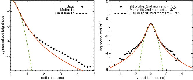
We first attempted to derive the PSF from the collapsed spectra of the monitor stars, which received the same exposure as the galaxies in the masks. The collapsed spectra were obtained by averaging over the flux in the wavelength direction, after masking skylines. The intensity profile had a very steep profile, which was superficially well fit by a Gaussian profile. Although adopting a Gaussian profile is common (e.g. Kriek et al. 2015), this was unexpected, because the MOSFIRE PSF in deep $K_{s}-$band imaging (Marchesini; private communication) clearly has strong wings, which generally are better fit with a Moffat profile (see Figure 2). Even small wings are important, because the effect of the PSF on convolution does not scale with the amount of flux in the wings, but with the second order moment of the PSF (Franx et al. 1989). Even a few percent flux in the wings can have a significant effect, due to the $r^{2}$ weighting. For illustration, we calculate the second moment for a simulated spectral PSF derived from a deep MOSFIRE image at FWHM$=0.6\arcsec$ seeing. The image PSF was created by median stacking 5 unsaturated bright stars, after background subtraction and normalization. First we measured the brightness profile of this two-dimensional PSF as a function of radius and fitted both a Moffat and a Gaussian function, as shown in the left panel of Figure 2. To reproduce the one-dimensional spectral PSFs, we integrated the two-dimensional image PSF and its two model fits within a 0.7″ virtual slit. Finally, we calculated the second order moments, $F_{2}$ for the PSF, $G_{2}$ for the Gaussian model and $M_{2}$ for the Moffat model. As shown in the right panel of Figure 2, the true PSF ($F_{2}=3.8$) is severely underestimated by a Gaussian approximation ($G_{2}=3.1$), whereas a Moffat fit produces good correspondence ($M_{2}=3.7$).

Figure 3.— Examples of spatial profiles of MOSFIRE PSFs. The solid and dashed curves are theoretically derived Moffat and Gaussian intensity profiles, respectively. They are shown at logarithmic scale in the left panel. A Moffat is a good representation of the original MOSFIRE PSF, but sky subtraction in the reduction process leaves negative imprints on each sides, which will subtract the strong wings. This makes the reduced PSF appear Gaussian. This is illustrated by the two examples of spatial profiles of monitor stars in the middle and right panels, with best and worst seeing, respectively. The black datapoints represent the star spectra collapsed in the wavelength direction. The solid and dashed lines are the reconstructed Moffat PSFs and the one-dimensional Gaussian fits, showing that they are nearly indistinguishable in one dimension.

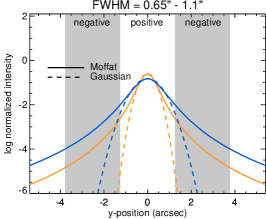
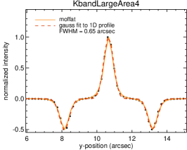
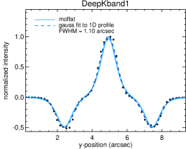
Clearly it is important to account for the flux in the wings of the PSF. However, it turns out to be rather difficult to reconstruct the true shape of the PSF accurately from the spatial profile of a monitor star spectrum. The reason is that standard reduction of the ABBA dither pattern results in one positive and two negative imprints each $2.52\arcsec$ apart, meaning the PSF wings are largely subtracted out and the resulting profile is too steep. The problem is seeing dependent and becomes worse if the seeing is larger. We therefore proceeded to reconstruct the true PSF separately for every mask (with seeing varying from 0.65 to 1.1″). As the central regions of the PSFs are still well approximated by a Gaussian, we used Gaussian fits to the collapsed spectra of the monitor stars to characterize the seeing FWHM for each of the 8 $K-$band masks. We then reconstructed the approximate true PSF by first integrating a two-dimensional Moffat ($\beta=2.5$) PSF over the width of a $0.7\arcsec$ wide virtual slit and subtracting 1/2 times the intensity offset by $2.52\arcsec$ on either side to simulate the reduction process. Because the FWHM of a Gaussian fit to the resulting spectral PSF is 12% broader than the original Moffat FWHM, we scaled the FWHM of the two-dimensional Moffat to match the simulated spectral PSF to the observations. Figure 3 illustrates two extreme cases of best and worst seeing for our data.

We verified the effect of using a Gaussian or Moffat profile in our modelling by calculating rotational velocities using either the Moffat PSFs derived above, or Gaussian fits to the collapsed star spectra. The mean velocity is 4% smaller if a Gaussian is assumed, with up to 15% effects for some individual cases.

2.2. Target sample selection

The primary ZFIRE sample was designed to spectroscopically confirm a large cluster of galaxies at $z=2.095$ (Spitler et al. 2012; Yuan et al. 2014) within the COSMOS field (Scoville et al. 2007). The sample was optimized by focusing mostly on near-IR star-forming galaxies, with strong expected signatures such as H$\alpha$ emission. Star-forming galaxies as part of the cluster were selected based on their rest-frame $U-V$ and $V-J$ colors, with photometric redshifts between $2.0<z<2.2$. $K$-band magnitudes of $K<24$ were priority sources, but fainter sources could be included as well. Non star-forming galaxies were prioritized next and lastly, field galaxies (not necessarily at the cluster redshift) could be used as fillers for the mask. In total 187 unique sources were listed for $K-$band observations. 36 of these were observed in two different masks and 2 in three different masks, leading to a total of 224 spectra.

Spectroscopic targets were originally obtained from the photometric redshift catalogs of ZFOURGE. These were derived from ultra-deep near-IR $K_{s}-$band imaging ($\sim 25.5$ mag). FourStar has a total of 6 near-IR medium bandwidth filters ($J_{1},J_{2},J_{3},H_{s},H_{l}$), that accurately sample the rest-frame $4000\mathrm{\AA}$/Balmer break at redshifts $1.5<z<4$. We combined these with a wealth of already public multiwavelength data at $0.3-24\micron$ to derive photometric redshifts, using the EAZY software (Brammer et al. 2008). These redshifts were used as a prior for the MOSFIRE masks. The typical redshift uncertainty is $1-2\%$ for galaxies at $1.0<z<2.5$ (Straatman et al. 2016).

For this work we make use of the ZFOURGE stellar masses. These were calculated by fitting Bruzual & Charlot (2003) stellar template models, using the software FAST (Kriek et al. 2009), assuming a (Chabrier 2003) initial mass function, exponentially declining star formation histories, solar metallicities and a Calzetti et al. (2000) dust law. Galaxy sizes, axis-ratios and position angles are obtained from the size catalog of galaxies from the 3D-HST/CANDELS survey (van der Wel et al. 2014a; Skelton et al. 2014). These were crossmatched to ZFOURGE by looking for matches within $<0.7\arcsec$. The sizes were derived by fitting two-dimensional Sérsic (Sersic 1968) surface brightness profiles to HST/WFC3/F160W images, using the software GALFIT (Peng et al. 2010).

From the original $N=224$ ZFIRE $K_{s}$-band sample, we first selected 151 unique galaxies with $2.0<z_{spec}<2.5$, where we used spectroscopic redshifts derived from one-dimensional collapsed spectra (Nanayakkara et al. 2016). Using the F160W position angles, we determined offsets with respect to the MOSFIRE masks: $\Delta\alpha=PA-\alpha_{mask}$, with PA the position angle of the major axis of the galaxy and $\alpha_{mask}$ the slit angle from the mask. We refined the sample by selecting only galaxies with $|\Delta\alpha|<40^{\circ}$ to minimize slit angle corrections, resulting in a sample of 81 galaxies. Some were included in more than one mask, and we have 102 spectra in total that follow these criteria. The H$\alpha$ emission was inspected by eye for contamination from sky lines, and we only kept those instances that were largely free from skylines, removing 25. Out of the remaining 77 spectra, 29 have very low SNR and were also omitted. We also looked for signs of AGN, by crossmatching with radio and X-ray catalogs (Cowley et al. 2016). This revealed one AGN, which we removed. Finally, we removed 5 spectra without corresponding HST/WFC3/F160W imaging. The final high quality sample contains 42 spectra of 38 galaxies, and these form the basis for the kinematic analysis which we discuss next.

3. Analysis

3.1. H$\alpha$ rotation model

We modeled the rotation curves by fitting two-dimensional ($\lambda,r$) intensity models. We used the empirically motivated arctan function to model the velocity curve (Courteau 1997; Willick 1999; Miller et al. 2011):

$$v(r)=V_{0}+\frac{2}{\pi}V_{a}\mathrm{arctan}\left(\frac{r-r_{0}}{r_{t}}\right)$$ (1)

with $v(r)$ the velocity at radius $r$, $V_{0}$ the central velocity, $V_{a}$ the asymptotic velocity, $r_{0}$ the dynamic center and $r_{t}$ the turnover, or kinematic, scale radius. $r_{t}$ is a transitional point between the rising and flattening of the arctan curve.

For relatively small proper motion if viewed on a cosmological scale, we can express the velocity as function of the wavelength difference with respect to the central wavelength $\lambda_{0}$ as:

$$\frac{v}{c}=\frac{\Delta\lambda}{\lambda_{0}}=\frac{\lambda-\lambda_{0}}{\lambda_{0}}$$ (2)

Therefore we initially fit our model in wavelength space, and then afterwards convert the offset in $\lambda$ to velocity. In terms of wavelength, Equation 1 becomes:

$$\lambda(r)=\lambda_{0}+\frac{2}{\pi}\lambda_{a}\mathrm{arctan}\left(\frac{r-r_{0}}{r_{t}}\right)$$ (3)

We also model the spatial intensity of the emission, assuming an exponential disk:

$$I(r)=I_{0}\mathrm{exp}\left[\frac{-(r-r_{0})}{R_{s}}\right]$$ (4)

with $I(r)$ the intensity at radius $r$ and $I_{0}$ the central intensity. $r_{0}$ is the same in Equations 1, 3 and 4, and the coordinates $(\lambda_{0},r_{0})$ represent the velocity centroid of the galaxy in H$\alpha$. $R_{s}$ is the scalelength of an exponential disk. At a given $r$, the intensity as a function of wavelength is modelled by a Gaussian profile, centered on $\lambda(r)$:

$$I(\lambda,r)=I(r)\mathrm{exp}\left[-\frac{(\lambda-\lambda(r))^{2}}{2(\sigma^{2}+\sigma_{instr}^{2})}\right]$$ (5)

with $\sigma$ the velocity dispersion and $\sigma_{instr}$ the instrumental broadening. $\sigma_{instr}=2.4\mathrm{\AA}$ was obtained from a Gaussian fit to a skyline. We allowed $\sigma$ to vary in the fit, but assumed it to be independent of radius.

With Equations 3 to 5 we built a two-dimensional model of the H$\alpha$ emission line, which was then smoothed with the PSF derived in Section 2.1.3. To avoid undersampling effects, we built the initial model on a grid with $3\times$ the spatial and wavelength resolution of the spectra. We also used a $3\times$ refined PSF. After convolving we rebinned the model by a factor $1/3$. We also subtracted half the intensity of the model at $\pm 14$ pixels to reproduce the dithering pattern. Parameters that can vary in the model are $\lambda_{0},\lambda_{a},r_{0},r_{t},I_{0},R_{s}$ and $\sigma$.

3.2. Fitting procedure

We fit the intensity model to $100\mathrm{\AA}$ wide spectral image stamps, centered on the H$\alpha$ emission line. We used the Python scipy optimize.curve_fit algorithm, which is based on the Levenberg-Marquardt algorithm. This algorithm can be used to solve non-linear least squares minimization problems. The Levenberg-Marquardt algorithm can find local minima, but these are not necessarily the global minima, i.e. the best fits, that we are looking for. Therefore, we assessed each galaxy’s spectral image stamp individually and we chose initial parameters for the model to be a reasonable match to the observed H$\alpha$ emission.

In addition to the H$\alpha$ stamps, we extracted corresponding images from the error spectra that are available for each observation. The error spectra represent standard errors on the flux in each pixel. The error stamps were matched by wavelength location to the H$\alpha$ spectral image stamps, and we included these as weight arrays in the fit. We did not mask sky lines or pixels with low SNR, but simply used the (much) smaller weights from the error images at those locations.

Figure 4.— Best-fit models. For each subsequent panel from left to right: the spectral image stamps, the best-fit model, the residual after subtracting the best-fit model. The blue dashed curves are the model arctan functions.

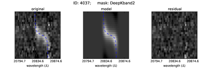
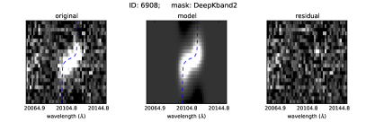
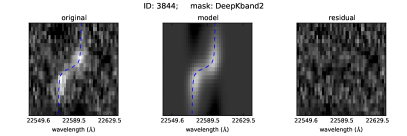
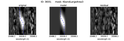
In Figure 4 we show the initial guesses and best-fit models for four example galaxies. The best-fit models are good representations of the H$\alpha$ emission, with small residuals. We also show the unconvolved arctangent functions constructed from the best-fit parameters using Equation 3. In Appendix A we show the spectral image stamps and best fits for the whole sample with additional radial velocity profiles derived from the emission in individual rows of each spectrum.

We estimated uncertainties on the parameters $\lambda_{0},\lambda_{a},r_{0},r_{t},I_{0},R_{s}$ and $\sigma$, by applying a Monte Carlo procedure. For every source, we subtracted the best-fit two-dimensional model from the spectral image stamp, obtaining the residual images shown Figure 4. We then shifted the residual pixels by a random number of rows and columns, preserving local pixel-to-pixel correlations. The magnitude of the shift was drawn from a Gaussian distribution centered on zero, allowing negative values, i.e., shifting in the opposite direction, and with a standard deviation of two pixels. The number of rows and columns to be shifted were generated independently from each other. We then added the best-fit model back to the shifted residual and re-ran our fitting procedure. We repeated this process 200 times, obtaining for each parameter a distribution of values. We calculated the standard deviations for each parameter and used these as the uncertainties.

3.3. Velocities

We measured the velocities from Equation 1 at 2.2 times the scale radius ($R_{s}$) of the exponential brightness profile. We chose $r=2.2R_{s}$ as this is the radius where the rotation curve of a self-gravitating ideal exponential disc peaks (Freeman 1970). It is also a commonly adopted parameter in literature (e.g. Miller et al. 2011). Its main advantage is that it gives a consistent approximation of the rotational velocity across the sample, while avoiding extrapolations towards large radii and low SNR regions of the spectrum.

We corrected the velocities for inclination using:

$$v^{\prime}_{2.2}=\frac{v_{2.2}}{\mathrm{sin}(i)}$$ (6)

with

$$i=\mathrm{cos^{-1}}\sqrt{\frac{(b/a)^{2}-q_{0}^{2}}{1-q_{0}^{2}}}$$ (7)

We adopt here the convention that $i=0^{\circ}$ for galaxies viewed face-on and $i=90^{\circ}$ for edge-on galaxies. We used the axis-ratio’s ($b/a$) derived with GALFIT from van der Wel et al. (2014a). Uncertainties on the axis-ratio were propagated and added to the velocity uncertainty from the Monte Carlo procedure.

$q_{0}\simeq 0.1-0.2$ represents the intrinsic flattening ratio of an edge-on galaxy. Following convention we adopt $q_{0}=0.19$ (Pizagno et al. 2007; Haynes & Giovanelli 1984). It has been shown that galaxies with $9<\mathrm{log}M/M_{\odot}<10$ at $z>1$ have a higher fraction of more elongated systems (e.g. van der Wel et al. 2014b). We note that using the axis-ratio’s to derive the inclination may therefore lead to underestimated corrections for some of the galaxies in our sample, as 9/21 have $\mathrm{log}M/M_{\odot}<10$.

3.4. Two-dimensional PSF and projection effects

When considering slit spectra, with one spatial dimension, we need to account for systematic effects due to the two-dimensional nature of the PSF smoothing as well as any mismatch between the slit angle and kinematic angle, here assumed to be the F160W position angle. The main effect is that two-dimensional smoothing will effectively lead to an underestimation of the line-of-sight motion captured in one-dimensional spectra, as a flux component from lower velocity regions is mixed in. The effect depends on the apparent size of the galaxy relative to the size of the PSF and the size of the slit, i.e., mixing occurs even for an infinitely thin slit if the seeing is significant, and vice versa.

To assess this effect, we generated a suite of 500 emission-line models (Bekiaris et al. 2016) of infinitely thin galaxies with similar sizes and velocities to our sample. We projected these onto the MOSFIRE 2D space, using various inclination angles ($0^{\circ}<i<90^{\circ}$) and slit angles relative to the major axes ($0^{\circ}<|\Delta\alpha|<45^{\circ}$), a finite slit width of $0.7\arcsec$, and a 2D Moffat PSF with FWHM$=0.5\arcsec$ and $\beta=2.5$. This PSF results in a Gaussian approximation of the seeing of $0.6\arcsec$ in 1D. In the simulations $R_{s}$ was varied between 1 and 5 kpc, $\sigma$ between 20 and 100 km/s and $V_{a}$ between 100 and 400 km/s. $r_{t}$ was defined as $R_{s}/3$, typical of the galaxies in this study. We added noise based on the noise spectrum of observed galaxy 4037 and scaled to match the typical H$\alpha$ SNR of the galaxies in our sample with a median of SNR$=25$ (see Section 3.5 for details on how we derive SNR). We included two negative imprints to simulate the ABBA pattern. The Bekiaris et al. (2016) models are part of a fitting code designed to diagnose IFU data and are therefore an excellent sanity check on methods used for single-slit modeling.

Figure 5.— Results of simulating 500 MOSFIRE spectra, with a 0.6$\arcsec$ PSF and typical SNR. We show the offset between input and measured velocity as a function of inclination, $|\Delta\alpha|$ and input $R_{s}$. The red lines are the running median and $1\sigma$ percentiles. There is a slight trend with inclination, indicating mixing of light plays a role, no trend with input $R_{s}$, and a strong trend with slit mismatch.

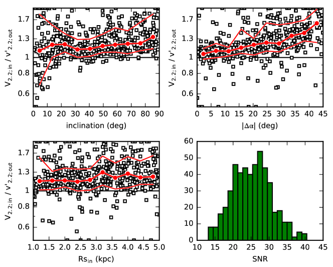
We measured the rotational velocity in the same way as for the observed spectra, including the correction for inclination angle. The ratio between $V_{2.2;in}$ (the actual rotational velocity) and $v^{\prime}_{2.2;out}$ (the measured rotational velocity) is shown in Figure 5. There is a slight trend with inclination, with on one side larger scatter for face-on galaxies, due to the general difficulties of measuring at small inclination. On the other side we find, as expected, an increase in both the scatter as well as the ratio $V_{2.2;in}/v^{\prime}_{2.2;out}$ for very inclined galaxies, that suffer the most from 2D smoothing effects. There is a strong trend of increasing $V_{2.2;in}/v^{\prime}_{2.2;out}$ towards higher $|\Delta\alpha|$, but we do not find a significant trend with input radius. In general the result is that the recovered velocities are too small by a median factor of 1.19, depending on $|\Delta\alpha|$, with a scatter of 0.24.

We found similar results for different seeing values or a factor 2 lower SNR. Given that there is a clear trend with slit angle mismatch, we derived a $|\Delta\alpha|-$dependent correction to our velocities, using the median offset in $V_{2.2;in}/v^{\prime}_{2.2;out}$ in a five degree bin around the value of $|\Delta\alpha|$ associated with each spectrum. We propagated the scatter around the median offset into the velocity uncertainty already derived from the Monte Carlo procedure. From hereon we use the symbol $V_{2.2}$ for the final slit angle and projection corrected velocities.

3.5. Results

Figure 6.— $K_{s}$-band magnitude and effective F160W radius $R_{e}$ stacked histograms of 38 galaxies in the high quality sample. For 18 spectra of 16 galaxies the fits were poorly constrained or could not be fit with an exponential brightness profile. The remaining 22 galaxies were used to derive the Tully-Fisher relation. The removed galaxies have fainter $K_{s}$-band magnitudes and smaller sizes on average, which resulted in a selection bias towards larger and/or brighter galaxies.

Table 1Results

ID	mask	seeing	$\mathrm{z_{centroid}}$	$V_{a}$	$r_{t}$	$R_{s}$	$\mathrm{SNR_{H\alpha}}$
		($\arcsec$)		(km/s)	($\arcsec$)	($\arcsec$)
1814	KbandLargeArea4	0.65	2.1704$\pm$0.00016	60.6$\pm$83.0	6.5e-10$\pm$1.3e-01	0.09$\pm$0.03	46
2715	mask2	0.67	2.0824$\pm$0.00004	52.3$\pm$90.5	8.2e-07$\pm$1.6e-01	0.16$\pm$0.03	22
2723	mask2	0.67	2.0851$\pm$0.00004	102.1$\pm$105.7	2.7e-06$\pm$1.6e-04	0.13$\pm$0.03	12
2765	mask1	0.71	2.2279$\pm$0.00008	242.6$\pm$83.2	3.5e-01$\pm$1.7e-01	0.24$\pm$0.03	36
3074	mask1	0.71	2.2267$\pm$0.00005	117.8$\pm$114.4	2.6e-02$\pm$2.6e-02	0.37$\pm$0.05	16
3527	KbandLargeArea4	0.65	2.1890$\pm$0.00004	87.9$\pm$3.2	1.6e-03$\pm$3.4e-04	0.23$\pm$0.01	71
3598	mask2	0.67	2.2279$\pm$0.00006	145.3$\pm$19.5	1.3e-01$\pm$3.6e-02	0.34$\pm$0.05	11
3633	DeepKband2	0.80	2.0991$\pm$0.00008	170.7$\pm$22.2	7.9e-02$\pm$2.8e-02	0.44$\pm$0.09	20
3655	KbandLargeArea3	1.09	2.1263$\pm$0.00003	110.0$\pm$31.5	2.2e-01$\pm$1.7e-01	0.35$\pm$0.06	41
3680	mask3	0.68	2.1753$\pm$0.00005	132.7$\pm$31.7	1.2e-01$\pm$6.4e-02	0.19$\pm$0.04	10
3714	mask3	0.68	2.1761$\pm$0.00005	81.1$\pm$76.7	2.1e-02$\pm$1.2e-02	0.22$\pm$0.01	33
3844	DeepKband2	0.80	2.4404$\pm$0.00001	177.5$\pm$181.8	1.2e-01$\pm$1.3e-01	0.70$\pm$0.02	16
4010	KbandLargeArea4	0.65	2.2216$\pm$0.00011	56.2$\pm$24.9	6.4e-09$\pm$2.3e-01	0.21$\pm$0.05	18
4037	DeepKband2	0.80	2.1750$\pm$0.00004	212.2$\pm$212.9	1.5e-01$\pm$1.5e-01	0.33$\pm$0.04	16
$-$	mask2	0.67	2.1747$\pm$0.00005	190.8$\pm$23.5	8.9e-02$\pm$3.0e-02	0.34$\pm$0.03	20
4099	mask3	0.68	2.4391$\pm$0.00002	51.1$\pm$52.0	1.3e-02$\pm$1.2e-02	0.28$\pm$0.03	15
4645	DeepKband1	1.10	2.1011$\pm$0.00005	184.7$\pm$27.7	1.7e-01$\pm$4.6e-02	0.26$\pm$0.03	3
4930	DeepKband2	0.80	2.0974$\pm$0.00002	70.4$\pm$27.6	1.5e-01$\pm$1.9e-01	0.24$\pm$0.03	14
5630	KbandLargeArea4	0.65	2.2427$\pm$0.00003	152.1$\pm$61.9	2.2e-01$\pm$2.2e-01	0.27$\pm$0.02	26
5870	mask4	0.66	2.1036$\pm$0.00006	51.7$\pm$8.6	3.2e-06$\pm$1.0e-02	0.20$\pm$0.05	18
6908	DeepKband2	0.80	2.0633$\pm$0.00002	145.8$\pm$17.1	8.3e-02$\pm$3.4e-02	0.30$\pm$0.02	19
$-$	mask1	0.71	2.0632$\pm$0.00004	144.4$\pm$142.5	4.1e-02$\pm$3.6e-02	0.33$\pm$0.05	26
8108	mask2	0.67	2.1622$\pm$0.00005	230.9$\pm$54.0	1.5e-01$\pm$5.8e-02	0.15$\pm$0.03	21
9420	mask3	0.68	2.0633$\pm$0.00016	344.0$\pm$337.2	4.2e-01$\pm$4.0e-01	0.28$\pm$0.05	5
ID	mask	$\sigma$	$v_{2.2}$	$V_{2.2}$	$V_{2.2;in}/v^{\prime}_{2.2;out}$	$\mathrm{sin}(i)$	$\alpha_{mask}$
		(km/s)	(km/s)	(km/s)		(deg)
1814	KbandLargeArea4	47.2$\pm$10.6	60.6$\pm$15.7	115.5$\pm$29.0	1.20$\pm$0.14	0.63	2.0
2715	mask2	57.0$\pm$5.6	52.3$\pm$11.5	72.2$\pm$15.3	1.11$\pm$0.08	0.81	-47.3
2723	mask2	69.4$\pm$6.1	102.1$\pm$7.4	283.4$\pm$46.2	1.36$\pm$0.23	0.49	-47.3
2765	mask1	83.6$\pm$11.0	150.2$\pm$29.4	242.0$\pm$68.0	1.26$\pm$0.31	0.78	134.0
3074	mask1	79.4$\pm$11.7	115.4$\pm$14.3	144.9$\pm$19.1	1.10$\pm$0.07	0.87	134.0
3527	KbandLargeArea4	68.4$\pm$4.1	87.7$\pm$3.3	107.2$\pm$7.5	1.09$\pm$0.07	0.89	2.0
3598	mask2	75.8$\pm$12.8	128.9$\pm$19.4	184.8$\pm$36.1	1.39$\pm$0.20	0.97	-47.3
3633	DeepKband2	52.2$\pm$4.9	161.9$\pm$19.3	202.9$\pm$29.1	1.19$\pm$0.12	0.95	-62.0
3655	KbandLargeArea3	27.3$\pm$10.5	90.5$\pm$10.9	288.2$\pm$39.6	1.10$\pm$0.09	0.35	59.0
3680	mask3	0.0$\pm$17.4	108.9$\pm$19.5	154.9$\pm$38.6	1.24$\pm$0.26	0.87	14.8
3714	mask3	70.2$\pm$4.4	78.9$\pm$7.4	130.9$\pm$15.6	1.19$\pm$0.11	0.72	14.8
3844	DeepKband2	52.8$\pm$4.5	168.6$\pm$3.1	251.5$\pm$22.8	1.10$\pm$0.11	0.73	-62.0
4010	KbandLargeArea4	104.6$\pm$9.8	56.2$\pm$14.1	72.8$\pm$18.1	1.10$\pm$0.11	0.85	2.0
4037	DeepKband2	21.9$\pm$8.9	185.1$\pm$9.2	283.0$\pm$29.4	1.10$\pm$0.11	0.72	-62.0
$-$	mask2	61.0$\pm$12.8	176.5$\pm$12.2	270.4$\pm$30.8	1.10$\pm$0.11	$-$	-47.3
4099	mask3	25.8$\pm$5.2	50.4$\pm$7.7	86.8$\pm$20.3	1.24$\pm$0.26	0.72	14.8
4645	DeepKband1	0.0$\pm$7.8	151.1$\pm$16.3	164.8$\pm$21.4	1.05$\pm$0.08	0.97	2.0
4930	DeepKband2	50.0$\pm$5.1	57.8$\pm$12.0	70.9$\pm$21.9	1.23$\pm$0.26	1.00	-62.0
5630	KbandLargeArea4	65.9$\pm$10.4	117.8$\pm$21.8	163.3$\pm$34.9	1.37$\pm$0.19	0.99	2.0
5870	mask4	21.1$\pm$10.1	51.7$\pm$6.9	74.9$\pm$11.6	1.10$\pm$0.11	0.76	-63.0
6908	DeepKband2	46.1$\pm$7.8	134.0$\pm$11.0	324.9$\pm$46.7	1.36$\pm$0.18	0.56	-62.0
$-$	mask1	86.9$\pm$11.3	139.3$\pm$22.0	298.0$\pm$53.7	1.20$\pm$0.15	$-$	134.0
8108	mask2	45.6$\pm$16.8	168.8$\pm$21.8	190.9$\pm$27.8	1.11$\pm$0.08	0.98	-47.3
9420	mask3	36.7$\pm$23.8	212.9$\pm$40.7	257.2$\pm$51.6	1.19$\pm$0.11	0.99	14.8

• Columns explained from left to right.

• ID: galaxy ID; mask: observing mask; seeing: measured gaussian seeing; $\mathrm{z_{cenroid}}$: redshift based on kinematic center; $V_{a}$: best-fit $V_{a}$; $r_{t}$ best-fit $r_{t}$; $R_{s}$: best-fit $R_{s}$; $\mathrm{SNR_{H\alpha}}$: signal-to-noise of the H$\alpha$ emission line; $\sigma$: best-fit intrinsic velocity dispersion; $v_{2.2}$: velocity derived at $2.2R_{s}$; $V_{2.2}$: velocity after correcting for inclination, projection effects and slit misalignment; $V_{2.2;in}/v^{\prime}_{2.2;out}$: median input versus output ratio of emission line models for the given $|\Delta\alpha|$; $\mathrm{sin}(i)$: inclination correction; $\alpha_{mask}$: slit angle.

• The final velocity was derived from $v_{2.2}$ as $V_{2.2}=(v_{2.2}/\mathrm{sin}(i))(V_{2.2;in}/v^{\prime}_{2.2;out})$.

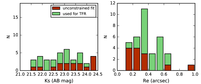
The best-fit parameters of the rotation model and their uncertainties, along with $v_{2.2}$ and $V_{2.2}$, are shown in Table 1. Of the 42 spectra in the high quality sample, we obtained good fits for 24 (of 22 galaxies), while for 18 spectra we obtained poorly constrained fits, with large random uncertainties ($>30\%$) on the velocities. We therefore removed these 18 spectra (of 16 galaxies) from the sample. To evaluate if removing the failed fits introduces biases relative to the target sample we show the distribution of the $K_{s}-$band magnitudes and sizes in Figure 6. The $K_{s}-$band magnitudes for the good fits are brighter than those of the full target sample (median $K_{s}=22.8$ versus median $K_{s}=23.5$) and the galaxies are slightly larger (median $R_{e}=0.40\arcsec$ versus $R_{e}=0.26\arcsec$). So removing these galaxies does bias the sample to somewhat brighter and larger galaxies.

The 22 galaxies for which we will derive the Tully-Fisher relation have high velocities and velocity dispersions, with a median $V_{2.2}=164$ km/s, $\sigma=53$ km/s and $V/\sigma=3$$.5$. We note that these dispersions could be slightly overestimated, e.g., the dispersion reflects mixing of velocity gradients on scales smaller than the seeing.

In case of high SNR the uncertainties are not dominated by random errors and the Monte Carlo procedure would result in relatively small errors. Because it is unlikely that we can derive velocities with more than 10% accuracy, we impose a minimum error of 10% of the measured velocities for all sources.

Figure 7.— Left: $R_{e}=1.678*R_{s}$ in the $K-$band from our fits versus $R_{e}$ in the HST/WFC3/F160W-band measured by van der Wel et al. (2014a), for 25 spectra. The dotted line indicates the one-to-one relation. Right: $\Delta R_{e}/R_{e;FIT}=(R_{e;FIT}-R_{e;3DHST})/R_{e;FIT}$ as a function of $R_{e,FIT}$. The bootstrapped median and $1\sigma$ error on the median (excluding any GALFIT bad fits indicated by red crosses) are shown as the solid and dashed blue lines, respectively.

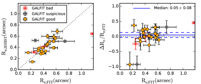
At high redshift measuring the kinematic profile of a galaxy is more difficult due to the smaller angular scales for distant galaxies, and seeing effects and SNR play a larger role. We therefore verified our size measurements. We converted the best-fit $R_{s}$ derived from the $K-$band spectra to effective radius ($R_{e}$), using $R_{e}=1.678R_{s}$ (valid for exponential disks), and compared this with the effective radii from HST/WFC3/F160W image reported by van der Wel et al. (2014a). On average we find good agreement, with some scatter, and we derived a bootstrapped median $\Delta R_{e}/R_{e}=0.05\pm 0.08$ (Figure 7). The most prominent outliers, with $|\Delta R_{e}/R_{e}|>0.5$, occur for two small galaxies, that have $R_{s}<25\%$ of the seeing. One additionally has a very irregular morphology, and was flagged by van der Wel et al. (2014a) as a suspicious GALFIT result.

We note that 7/25 fits resulted in very small $r_{t}$, with $r_{t}<0.02\arcsec$. This is clearly much less than the resolution of a pixel: $0.18\arcsec$. To investigate the potential impact of small $r_{t}$ on the velocities, we re-fit these spectra limiting $r_{t}$ to $r_{t}>0.02\arcsec$, obtaining a median velocity that is 10% higher. This may indicate that the velocities are underestimated for sources with small $r_{t}$, but without knowing the true $r_{t}$, the effect is difficult to quantify.

The total SNR is included in Table 1. We measured the SNR within $5R_{s}$ above and below the center of the line, but never beyond $1.26\arcsec$ to avoid the negative imprints of the emission line in the spectrum. We also defined a wavelength region within which to measure SNR, defined by the maximum shear of the line, plus a buffer of $3FWHM_{\lambda}=3(2\sqrt{2\mathrm{ln}2})\sqrt{\sigma^{2}+\sigma_{instr}^{2}}\mathrm{\AA}$. The SNR within these limits was calculated by summing the flux and summing the squares of the equivalent pixels in the noise spectrum, and dividing the first by the square root of the latter.

Two galaxies were included in two masks (4037 and 6908 in Table 1). As they were observed under different seeing conditions and have different SNR and slit-angle, they provide a useful check on consistency. Encouragingly, we find that these galaxies have velocities, redshifts and scale parameters that agree between masks within their uncertainties. We averaged their velocities to derive the Tully-Fisher relation in the next Section.

4. The Tully-Fisher relation at $2.0<z<2.5$

4.1. Tully-Fisher sample

Figure 8.— HST/WFC3/F160W images of the galaxies in our Tully-Fisher sample. The green box shows the dimensions and orientation of the slit compared to the galaxies. The dotted line indicates the PA of the major axis.

Table 2Full sample

ID	R.A.	Decl	$\mathrm{K_{s}}$	F160W	$\mathrm{M/10^{10}}$	SFR	$R_{e}$	GALFIT	$b/a$	$n_{sersic}$	P.A.
	(deg)	(deg)	(AB mag)	(AB mag)	$\mathrm{(M_{\odot})}$	$\mathrm{(M_{\odot}/yr)}$	($\arcsec$)	flaga			(deg)
1814	150.1680908	2.2112861	23.0	23.3	0.6	17.5	0.31$\pm$0.01	0	0.79$\pm$0.02	0.6	-17.6
2715	150.0895386	2.2235634	22.6	23.0	0.8	34.4	0.52$\pm$0.02	1	0.61$\pm$0.03	0.6	-37.9
2723	150.1172638	2.2238791	21.5	22.0	7.8	66.4	0.14$\pm$0.00	0	0.88$\pm$0.02	4.5	-13.6
2765	150.119339	2.2241209	21.9	22.5	2.4	101.1	0.29$\pm$0.01	0	0.64$\pm$0.01	1.8	-73.9
3074	150.1209106	2.2288201	22.2	22.6	1.4	30.9	0.69$\pm$0.04	0	0.51$\pm$0.02	2.3	-59.2
3527	150.1825714	2.2358665	21.9	22.5	2.1	168.8	0.39$\pm$0.01	0	0.48$\pm$0.01	1.0	-9.5
3598	150.1120911	2.2368469	22.9	23.7	2.3	69.9	0.59$\pm$0.05	0	0.30$\pm$0.03	1.1	-10.0
3633	150.1249237	2.236979	22.1	22.7	2.5	150.5	0.51$\pm$0.02	1	0.37$\pm$0.02	0.9	-84.5
3655	150.1691284	2.2383816	21.9	22.4	2.1	127.3	0.56$\pm$0.01	0	0.94$\pm$0.01	1.1	44.7
3680	150.063446	2.237031	24.0	24.1	0.2	16.9	0.34$\pm$0.02	0	0.51$\pm$0.04	0.9	-10.2
3714	150.0707703	2.2381561	22.7	23.3	1.5	23.1	0.33$\pm$0.01	0	0.71$\pm$0.02	0.7	-6.3
3844	150.1094666	2.2400432	22.4	23.0	1.5	65.2	0.64$\pm$0.02	2	0.69$\pm$0.02	0.2	-68.3
4010	150.1798706	2.2423265	23.0	23.5	1.1	131.2	0.28$\pm$0.01	0	0.55$\pm$0.02	0.4	-5.8
4037	150.0981293	2.2428052	22.2	23.1	4.9	95.7	0.39$\pm$0.01	0	0.71$\pm$0.02	0.6	-54.8
4099	150.0718231	2.243396	23.1	23.7	2.2	57.5	0.46$\pm$0.04	0	0.71$\pm$0.03	1.7	-10.6
4645	150.0743256	2.2516196	23.6	23.8	0.3	14.1	0.33$\pm$0.01	0	0.32$\pm$0.03	0.5	-0.5
4930	150.0559387	2.2557058	23.5	23.8	0.3	15.3	0.41$\pm$0.02	2	0.09$\pm$0.02	0.2	87.6
5630	150.2009735	2.2665324	22.9	23.3	0.9	111.3	0.44$\pm$0.03	0	0.24$\pm$0.02	2.4	-34.9
5870	150.0609436	2.2696433	23.1	23.5	0.8	15.2	0.38$\pm$0.02	0	0.67$\pm$0.02	0.7	-71.0
6908	150.0834198	2.2857671	21.7	22.2	3.0	138.9	0.51$\pm$0.01	0	0.84$\pm$0.01	0.4	-25.6
8108	150.0622711	2.3044007	23.8	24.1	0.5	16.3	0.31$\pm$0.02	2	0.27$\pm$0.03	0.2	-37.3
9420	150.0947418	2.3236084	23.6	24.0	0.7	17.1	0.60$\pm$0.03	0	0.24$\pm$0.03	0.5	36.3

• Columns explained from left to right.

• ID: galaxy ID; R.A.: right ascension; Decl: declination; K_s: total FourStar/K${}_{s}-$band magnitude; F160W: total HST/WFC3/F160W magnitude; M: stellar mass; SFR: star-formation rate; $R_{e}$: effective radius from van der Wel et al. (2014a); GALFIT flag: quality flag provided by van der Wel et al. (2014a); $b/a$: axis ratio: $n_{sersic}$: sersic index; P.A.; position angle of the major axis.

• 0: good fit; 1: suspicious fit; 2: bad fit (van der Wel et al. 2012).

Figure 9.— Rest-frame $U-V$ colours, stellar masses and ZFOURGE $K_{s}$-band magnitudes for the 22 galaxies used here to derive the Tully-Fisher relation (green), the ZFIRE target sample (lightblue), and a parent sample drawn from ZFOURGE with $2<z<2.5$ and $M/M_{\odot}>10^{9}$ (gray). The gray histograms were reduced by a factor of three for reasons of visibility. The 22 galaxies of this study have a large range in $U-V$, stellar mass and brightness.

Figure 10.— Left: UVJ diagram of the ZFIRE sample (open symbols) and the 22 galaxies studied in this work (squares). The underlying histogram is the full distribution of $2.0<z<2.5$ galaxies with $M>10^{9}$ $\mathrm{M_{\odot}}$from ZFOURGE. This diagram separates quiescent galaxies from star-forming galaxies based on their rest-frame $U-V$ and $V-J$ colors, obtained from ZFOURGE photometry. The 22 galaxies in the sample span the full range in color typical of star-forming galaxies (region below the red line). Middle: stellar mass versus the logarithm of SFR. The orange line shows the median SFR as function of stellar mass of star-forming galaxies at $2.0<z<2.5$ (Tomczak et al. 2015). Most of the galaxies in the sample are above the SFR-stellar mass relation at that redshift (Tomczak et al. 2015). Right: stellar mass versus effective radius, with the size-mass relation at $2.0<z<2.5$ for star-forming galaxies shown as a blue line. The dashed lines are the corresponding 16th and 84th percentiles. Open square datapoints are flagged as suspicious or bad fits in the catalogs of van der Wel et al. (2014a).

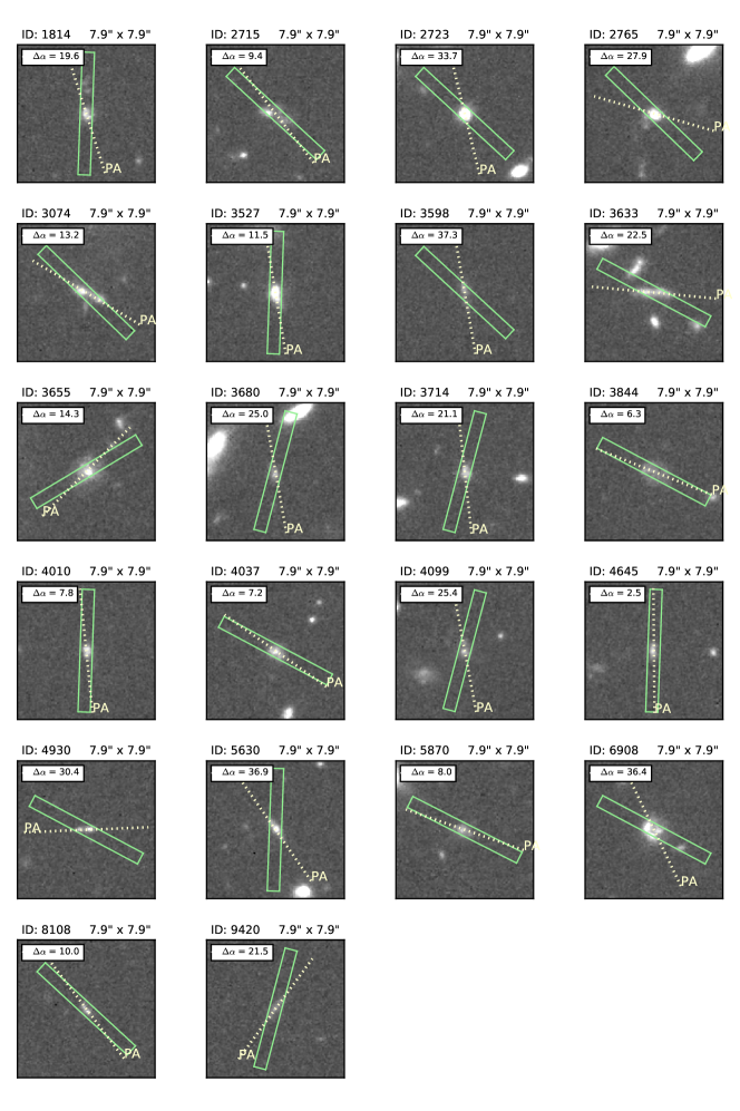
We show F160W images of the remaining 22 galaxies in the Tully-Fisher sample in Figure 8, and illustrate the orientation of their major axis and the MOSFIRE slits. Physical properties of the sample are shown in Table 2, Figure 9 and Figure 10. We also compare with the primary 187 ZFIRE targets as well as with the general population of galaxies at this redshift obtained from ZFOURGE. For the ZFOURGE sample we selected galaxies with stellar mass $M/M_{\odot}>10^{9}$. The 19 galaxies in our sample cover the full range of the star-forming region of the UVJ diagram (below the red line), but they have higher star-formation rates (SFRs) compared to the SFR-stellar mass relation for star-forming galaxies at $2.0<z<2.5$ (Tomczak et al. 2015). They lie at the bright, high-mass end of the general galaxy population. They have a large spread in size (Figure 10), including even a massive compact galaxy with effective size $R_{e}=0.14\arcsec$, but on average they are larger than predicted by the size-mass relation at $2.0<z<2.5$ (van der Wel et al. 2014a).

Of the 22 galaxies, 6 are spectroscopically confirmed to be part of the $z=2.095$ galaxy cluster. However, due to the small number of cluster galaxies in this sample, a study of the effects of environment on the evolution of the Tully-Fisher relation is not feasible here. Alcorn et al. (2016) measured the velocity dispersions of a larger sample of ZFIRE cluster galaxies and found no evidence for environmental effects at this redshift.

4.2. The Tully-Fisher relation

Table 3Tully-Fisher variables

ID	$V_{2.2;TF}$	$S_{05;TF}$	$\sigma_{TF}$
	(km/s)	(km/s)	(km/s)
1814	115.5$\pm$29.0	94.4$\pm$18.5	47.2$\pm$10.6
2715	72.2$\pm$15.3	76.5$\pm$8.3	57.0$\pm$5.6
2723	283.4$\pm$46.2	212.1$\pm$31.0	69.4$\pm$6.1
2765	242.0$\pm$68.0	190.4$\pm$43.5	83.6$\pm$11.0
3074	144.9$\pm$19.1	129.6$\pm$12.9	79.4$\pm$11.7
3527	107.2$\pm$10.7	102.1$\pm$6.3	68.4$\pm$4.1
3598	184.8$\pm$36.1	151.1$\pm$23.0	75.8$\pm$12.8
3633	202.9$\pm$29.1	152.7$\pm$19.4	52.2$\pm$4.9
3655	288.2$\pm$39.6	205.6$\pm$27.8	27.3$\pm$10.5
3680	154.9$\pm$38.6	109.5$\pm$27.3	0.0$\pm$17.4
3714	130.9$\pm$15.6	116.2$\pm$9.2	70.2$\pm$4.4
3844	251.5$\pm$25.2	185.5$\pm$17.1	52.8$\pm$4.5
4010	72.8$\pm$18.1	116.6$\pm$10.5	104.6$\pm$9.8
4037	276.7$\pm$42.6	200.0$\pm$29.7	41.5$\pm$15.6
4099	86.8$\pm$20.3	66.6$\pm$13.4	25.8$\pm$5.2
4645	164.8$\pm$21.4	116.5$\pm$15.1	0.0$\pm$7.8
4930	70.9$\pm$21.9	70.8$\pm$11.5	50.0$\pm$5.1
5630	163.3$\pm$34.9	132.9$\pm$22.1	65.9$\pm$10.4
5870	74.9$\pm$11.6	57.0$\pm$8.5	21.1$\pm$10.1
6908	311.5$\pm$71.2	230.1$\pm$48.4	66.5$\pm$13.7
8108	190.9$\pm$27.8	142.5$\pm$19.4	45.6$\pm$16.8
9420	257.2$\pm$51.6	185.5$\pm$36.1	36.7$\pm$23.8

• $V_{2.2;TF}$, $S_{05;TF}$ and $\sigma_{TF}$ were used to generate Figure 11. For sources with observations in multiple masks, they are average values.

Figure 11.— Left: Stellar mass versus velocity and the best-fit Tully-Fisher relation for galaxies at $2.0<z<2.5$: $\mathrm{log}V_{2.2}=$$(2.18\pm 0.051)$$+$$(0.193\pm 0.108)$$(\mathrm{log}M/M_{\odot}-10)$ (blue line). For comparison, the dashed purple line is the $z\sim 2.2$ result from (Cresci et al. 2009). The dash-dotted and dotted lines are the $z=0$ results from Reyes et al. (2011) and Bell & de Jong (2001), respectively. The green and orange lines are the best-fit results with the slope fixed to the respective slopes at $z=0$. The scatter in velocity around the relation is 0.19 dex. Right: Stellar mass versus $S_{0.5}=\sqrt{0.5V_{2.2}^{2}+\sigma^{2}}$. The scatter in $S_{0.5}$ is smaller than in velocity: 0.16 dex. We derive a best-fit relation $\mathrm{log}S_{0.5}=(2.07\pm 0.03)+(0.224\pm 0.060)(\mathrm{log}M/M_{\odot}-10)$ (red line), with a steeper slope than at $0.1<z<1.2$ (dash-dotted line; Kassin et al. 2007). The solid red line is the best-fit with the slope fixed to match the relation of Kassin et al. (2007). The red dotted line shows the same result if we remove the smoothing and slit misalignment corrections and assume a Gaussian PSF (velocities 4% smaller).

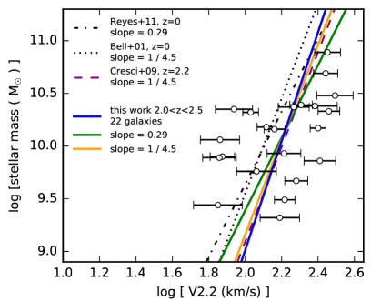
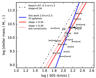
The Tully-Fisher relation is the relation between rotational velocity and stellar mass. We show our rotation measurements (also shown in Table 3) versus stellar mass in the left panel of Figure 11, using the stellar masses taken from the ZFOURGE catalogs and averaging values if galaxies were observed in two masks. We performed a linear regression to the data following:

$$\mathrm{log}V_{2.2}=B+A(\mathrm{log}M/M_{\odot}-10)$$ (8)

The Tully-Fisher relation is by convention shown in diagrams with stellar mass on the y-axis. However, the dominant uncertainty here is that in velocity and therefore we performed regression with $V_{2.2}$ as the dependent variable. This is also a method very commonly used in literature which acts against Malmquist bias (Bamford et al. 2006; Weiner et al. 2006b; Kelly 2007).

We obtain from the fit $B=$$(2.18\pm 0.051)$ and $A=$$(0.193\pm 0.108)$. We derived the uncertainties by bootstrapping the sample 1000 times, and taking the standard deviation from the bootstrapped distributions of $B$ and $A$. The slope of the Tully-Fisher relation, $(0.193\pm 0.108)$, is consistent with previous results at $z=0$. For example, Reyes et al. (2011) find $A=0.29$ and Bell & de Jong (2001) find $A=1/4.5=0.22$. Our study has too few numbers to significantly constrain evolution in the slope between $z=0$ and $2<z<2.5$, but if we fix the slope to that at lower redshift we can study the evolution of the zeropoint. Setting $A=0.29$, we find $B=$$(2.17\pm 0.047)$. Compared to $z=0$ (Reyes et al. 2011), this implies an evolution of the zeropoint (in stellar mass) of $\Delta\mathrm{M}/$$\mathrm{M_{\odot}}$$=-0.25\pm 0.16$ dex. We included here a small correction of -0.05 dex in stellar mass to account for the Kroupa (2001) IMF used by Reyes et al. (2011) instead of the Chabrier (2003) IMF used here. Similarly, we can compare to the $z=0$ result of Bell & de Jong (2001), by setting the slope to 1/4.5. This results in an observed evolution of $\Delta\mathrm{M}/$$\mathrm{M_{\odot}}$$=-0.39\pm 0.21$ dex. These offsets in steller mass are consistent with the findings of Cresci et al. (2009) and Simons et al. (2016) who derived $\mathrm{\Delta M/M_{\sun}}=-0.41\pm 0.11$ dex and $\mathrm{\Delta M/M_{\sun}}=-0.44\pm 0.16$, respectively.

As an additional consistency check, we investigated the effects of sample selection. First we refined the sample even more and we fitted the Tully-Fisher relation only to the galaxies with highest SNR, fixing the slope to $A=0.29$ or 1/4.5. We obtained consistent results with $\Delta\mathrm{M}/$$\mathrm{M_{\odot}}$$=-0.27\pm 0.17$ dex and $\Delta\mathrm{M}/$$\mathrm{M_{\odot}}$$=-0.43\pm 0.23$ dex, respectively, for the 11 galaxies with spectra with SNR$>20$. Then we tested applying a less severe sample selection, including spectra with velocity errors $<50\%$ instead of $<30\%$. This resulted in $\Delta\mathrm{M}/$$\mathrm{M_{\odot}}$$=-0.18\pm 0.16$ dex and $\Delta\mathrm{M}/$$\mathrm{M_{\odot}}$$=-0.29\pm 0.21$ dex, respectively, for a sample of 27 galaxies. This is a rather large difference and we take note that it may be a potential caveat if one selects the brightest (and therefore easiest to fit) galaxies.

Figure 12.— Difference between the observed velocity and the velocity predicted by the best-fit Tully-Fisher relation. We plot against model and observational parameters. From left to right, top to bottom: SNR, log $V_{2.2}$, log stellar mass, best-fit $R_{s}$, best-fit $r_{t}$, best-fit $\sigma$, redshift, inclination, $\Delta\alpha$, Sersic index, SFR, SFR minus predicted SFR at $2.0<z<2.5$ (Tomczak et al. 2015), SSFR, seeing and $R_{s}$ relative to the seeing. We find almost no correlations, except for best-fit $r_{t}$, with a negative offset in $\Delta$log$V_{2.2}$ for fits with $r_{t}\approx 0$.

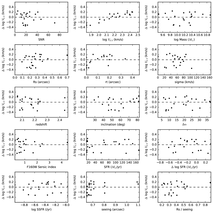
To investigate if there are remaining systematic trends we show in Figure 12 the velocity residuals of the best-fit Tully-Fisher relation with respect to various parameters and properties of the galaxies (such as SFR). We define the residual as $\Delta\mathrm{log}V_{2.2}=\mathrm{log}V_{2.2}-\mathrm{log}V_{TFR}$ with $V_{TFR}$ the rotational velocity predicted from the fit for a specific stellar mass. There are no systematic effects related to Sersic Index, $R_{s}$, stellar mass, SFR, specific SFR (SSFR), or offset from the SFR-stellar mass relation at $2.0<z<2.5$ (Tomczak et al. 2015). In addition there is no clear relation with inclination, PA, or seeing. A few prominent outliers have a negative $\Delta\mathrm{log}V_{2.2}$, i.e., they are located to the left of the Tully-Fisher relation in Figure 11. These have average values of very small $r_{t}$, the kinematic scale radius. As we have shown in Section 3.3, resolution effects may play a role in determining $r_{t}$, and we derive somewhat higher velocities if we limit $r_{t}$ to $r_{t}>0.02\arcsec$ for these spectra, resulting in $\Delta\mathrm{log}M/M_{\odot}=-0.31\pm 0.14$ dex and $\Delta\mathrm{log}M/M_{\odot}=-0.47\pm 0.17$ dex for slopes of 0.29 and 1/4.5, respectively, for the whole sample. We note that a value of zero for $r_{t}$ is possible in the presence of non-circular motion, for example if the galaxy has a bar (Franx & de Zeeuw 1992). We inspected the F160W images, but found no indications of a bar-like morphology.

The scatter of the residual velocities with respect to the Tully-Fisher relation is significant, with $\sigma=0.19$ dex. This is more than at $z=0$, and could partly be due to the low $r_{t}$ outliers. It may also be related to star-forming galaxies at high redshift showing more variety in kinematics, and the increase of non-rotationally supported galaxies (e.g. Kassin et al. 2007). An alternative to the stellar mass-velocity relation is the stellar mass-$S_{0.5}$ relation, with $S_{0.5}=\sqrt{0.5V_{2.2}^{2}+\sigma^{2}}$. This relation was first coined by Weiner et al. (2006a), and Kassin et al. (2007) showed that the scatter decreases significantly if $S_{0.5}$ is used. They also found that it does not evolve significantly between $z=0.1$ and $z=1.2$.

We calculated $S_{0.5}$ for the galaxies in our sample (right panel in Figure 11) and find the scatter is indeed smaller: $\sigma_{rms}=0.15$ dex, similar to what Kassin et al. (2007) derived at $0.1<z<1.2$ (0.16 dex) and to a recent study by Price et al. (2015), using MOSFIRE at $1.4<z<2.6$ (0.17 dex). We derived the best-fit relation to the data with $A$ and $B$ free in the fit and found $\mathrm{log}S_{0.5}=$$(2.06\pm 0.032)$$+$$(0.211\pm 0.086)$$(\mathrm{log}M/M_{\odot}-10)$. Here the slope is steeper than at $0.1<z<1.2$, where Kassin et al. (2007) found that $A=0.34$. This is in agreement with the previous study by Cresci et al. (2009), who did not derive a best-fit to their data, but they do find higher $S_{0.5}$ values towards smaller stellar mass compared to the $0.2<z<1.2$ relation. Keeping the slope fixed at $A=0.34$, we found $B=$($2.03\pm 0.032$). This implies a zeropoint evolution of $\Delta\mathrm{M}/$$\mathrm{M_{\odot}}$$=-0.45\pm 0.13$ dex compared to $0.1<z<1.2$. Price et al. (2015) also find an offset in $\Delta\mathrm{M}/$$\mathrm{M_{\odot}}$ for galaxies at high redshift, implying $\Delta\mathrm{M}/$$\mathrm{M_{\odot}}$$\sim-0.3$ dex, and their data does not indicate a steeper slope. Their offset from $0.1<z<1.2$ is inconsistent with and less than what we find, which could be due to the inclusion of galaxies at $z<2$, their assumption of a Gaussian PSF, and our correction for two-dimensional PSF effects. If we account for the Gauss-Moffat difference and remove the correction for smoothing and slit misalignment, the inferred evolution compared with $z<1.2$ is less: $\Delta\mathrm{M}/$$\mathrm{M_{\odot}}$$=-0.26\pm 0.12$ dex. Both the findings from Price et al. (2015) and ours point towards evolution of the zeropoint of the stellar mass-$S_{0.5}$ relation between $z<1.2$ and $z\gtrsim 2$, but no evolution for the scatter in $S_{0.5}$.

One caveat could be the possible misclassification of mergers as rotating disks in our sample. As Hung et al. (2015) showed using artificially redshifted IFU data, a large fraction of high redshift ($z>1.5$) interacting galaxies would still be kinematically classified as single rotating disks. Inspection of Figure 8 indicates that some of the galaxies here have multiple components with small angular separations, e.g., #1814, #4930, #6908. Such components may contribute differently to the kinematics of the system, but to investigate this in detail is beyond the scope of this paper.

5. Discussion

5.1. Comparison to literature

Figure 13.— The evolution of the stellar mass zeropoint with redshift. The yellow datapoints represent the observed evolution from our survey at $2.0<z<2.5$ for fixed slopes of 0.29 (left panel) or 1/4.5 (right panel). Uncertainties are derived from bootstrap resampling and the horizontal error bar indicates the standard deviation of redshift in our sample. Results from other surveys (as quoted in the corresponding papers) are shown with symbols as indicated in the legend. For studies that do not compare directly with Bell & de Jong (2001) or Reyes et al. (2011) we use gray symbols. The magnitude of the systematic effects that we have corrected for are indicated by arrows, and we have also indicated the magnitude of a factor 2 uncertainty in stellar mass with a vertical errorbar (M). We also show the predictions from semi-analytical models (pink lines).

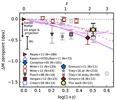
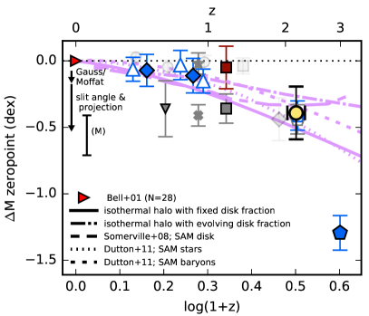
To put our result into context, we show the evolution of the stellar mass zeropoint in Figure 13, and include previous results from literature. These were all derived from the stellar mass-velocity relation, with quite strong discrepancies between different studies at $z>0.5$. However, before comparing with other studies at different redshifts, several major caveats have to be taken into account: studies use different galaxy selections, different methodologies to derive velocity and stellar mass, and different types of spectroscopic observations. We will discuss these first and then review and compare the studies.

The first is selection bias. At $z>2$ star-forming galaxies have different properties on average than at $z=0$. For example, they have higher SFRs, higher gas masses and smaller sizes (e.g. Papovich et al. 2015; van der Wel et al. 2014a). At $z>2$ dust-obscured galaxies are more common, and for these galaxies the H$\alpha$ luminosity is attenuated (e.g. Reddy et al. 2005; Spitler et al. 2014). Samples that are UV or H$\alpha$ selected may therefore not be a complete distribution of star-forming galaxies at high redshift and changes in incompleteness may mimick evolution with redshift. Mergers and galaxies with irregular morphologies are also more common than at $z=0$ (e.g. Abraham & van den Bergh 2001; Mortlock et al. 2013). These galaxies have less ordered velocity fields (e.g. Kassin et al. 2007) higher velocity dispersions relative to circular velocities, and are often excluded from Tully-Fisher samples because it is difficult to describe these galaxies with smooth rotating models (Cresci et al. 2009; Gnerucci et al. 2011). At high redshift the angular extent of galaxies is often small compared to the seeing, which may give the appearance that the galaxy is dispersion dominated if the velocity gradient is unresolved (e.g. Miller et al. 2012). If the selection requires ordered rotation, this leads to biases towards larger galaxies.

Here we have attempted to introduce as little selection bias as possible, but it could not be entirely avoided. As described in Section 3.5, we have excluded galaxies with poor fits, which tended to be galaxies with smaller sizes and fainter magnitudes than the overall photometric sample. Despite the large uncertainties on the velocities of these poor fits, in Section 4.2 we have shown that such a selection may indeed bias the result towards larger average velocities and hence a stronger evolution of the stellar mass zeropoint.

Another caveat when comparing different results from literature is methodology. In many studies the PSF is assumed to be Gaussian, but for our MOSFIRE data a Moffat profile is a better approximation. The difference between using a Gaussian and a Moffat in our modelling leads to a 0.06$-0.08$ dex shift in the stellar mass zeropoint of the Tully-Fisher relation, depending on the slope. In addition, several different possibilities exist to model the velocity field, e.g. the one-dimensional arctan model we used here (and also used by e.g. Miller et al. 2011, 2012) or a two-dimensional integrated mass model (Cresci et al. 2009; Gnerucci et al. 2011). Different choices for the radius at which to evaluate velocity exist as well. In some cases $R_{80}$ is used, encapsulating 80% of the optical light (Reyes et al. 2011). In other cases $V_{max}$ is used, or the asymptotic velocity $V_{a}$ in the arctan model, which is often extrapolated at a radius beyond the optically observed extent of the galaxy (e.g. Weiner et al. 2006b). Most studies in Figure 13 employ $V_{max}$. We prefer $V_{2.2}$, because it is more robust, and it is used in several other studies (e.g. Miller et al. 2011, 2012). The relation Reyes et al. (2011) derived for $V_{80}$, which is close to $V_{max}$, implies a 4% increase in velocities relative to $V_{2.2}$, or a $\sim 0.06$$-0.08$ dex effect on the inferred stellar mass zeropoint. Lastly, uncertainty on the stellar mass has to be taken into account. We derived our stellar mass from fitting to SEDs obtained from photometry, which depends on several assumptions of the stellar population models. Differences between a Salpeter (1955), Kroupa (2001), Diet Salpeter (Bell et al. 2003) and Chabrier (2003) IMF are $0.05-0.3$ dex. In addition, different stellar populations models can produce stellar masses different by a factor of 2 (e.g. the review of Conroy 2013). Also, fitting models to SEDs versus applying M/L ratios based on ($g-r$) colors (Bell et al. 2003; Puech et al. 2008) can amount to up to a factor of 2 differences (Reyes et al. 2011).

Another important issue is simply that the datasets between surveys are of a different kind, such as single-slit data versus integral field spectroscopy. For example, Cresci et al. (2009), who use IFS, employ a three-dimensional method, by modelling a datacube with x,y and $\lambda$ dimensions. This kind of modelling already includes effects from the two-dimensional PSF and projection, whereas (y,$\lambda$) modelling of single-slit data using a one-dimensional PSF (as performed in this study and by Conselice et al. (2005); Kassin et al. (2007); Miller et al. (2011, 2012) at high redshift) results in systematically underestimating the velocity.

In summary, methodology and data sets can introduce significant velocity offsets. Reviewing the studies at different redshifts with this in mind we can try to understand these discrepancies. For example, there exist clear differences between Puech et al. (2008) and other studies (e.g. Conselice et al. 2005; Kassin et al. 2007; Miller et al. 2011) at $z\sim 0.5$ of $0.3-0.4$ dex. There is also a strong apparent evolution between $z=1.7$ (Miller et al. 2012, based on one-dimensional modeling of single-slit data) and our results at $z=2.2$. This can at least in part be explained if we take into account our slit misalignment and projection corrections (see Section 3.4). For example, Weiner et al. (2006a) already speculated velocities may become underestimated for larger $|\Delta\alpha|$ and based on this Kassin et al. (2007) select sources with $|\Delta\alpha|<40^{\circ}$, but do not correct for slit misalignment. In Section 3.4 however we showed that the effects of slit misalignment are still strong even for $|\Delta\alpha|<40^{\circ}$. Miller et al. (2011) and Miller et al. (2012) apply a correction for slit misalignment (Miller et al. 2011, Equation 4), but if we apply the same to our simulations, we still find a residual $V_{2.2;in}/v^{\prime}_{2.2;out}=1.1$, independent of $|\Delta\alpha|$. We show the median correction applied to our data in both panels of Figure 13. It is likely that a similar correction is applicable to all single-slit studies based on one-dimensional modeling, but we also note that such corrections are dependent on slitwidth as well as the angular size of a galaxy. The effect may thus be smaller at $z<2$. Encouragingly, Harrison et al. (2017) derive a similar median correction of 7% on circular velocites measured in virtual single slits projected on IFU data of $z\sim 0.9$ galaxies. The differences at $z=0.6$ with the result from Puech et al. (2008) may further be explained by a different conversion from light to stellar mass (M/L ratios versus SED fitting).

The effects of sample selection on the observed evolution have been shown by Tiley et al. (2016), who measured the stellar mass Tully-Fisher relation both for a parent sample of more general properties, e.g., H$\alpha$ detected, non-zero rotation with $<30\%$ uncertainties, as well as for a subsample of rotation dominated galaxies with $v/\sigma>3$. They found a $\Delta\mathrm{M}/$$\mathrm{M_{\odot}}$$=0.39$ dex difference, with stronger evolution for the rotation dominated sample. The median $V_{2.2}/\sigma$ of our sample is 3.5 and we must keep in mind that our sample may trace the evolution of the more rotationally supported disks. The differences between $0<z<2$ studies and the $z=3$ result of Gnerucci et al. (2011) could be related to their rest-frame UV selection and requirement of optical (rest-UV) spectroscopic redshifts, which tends to be much bluer than near-IR selected samples at $1<z<2$.

Different studies also compare to different $z=0$ relations. The most common references are the results from Bell & de Jong (2001), Pizagno et al. (2005), and Reyes et al. (2011). These are based on different IMF, choice of velocity indicator, and method to derive stellar mass. In most high redshift studies, estimates of the evolution of the Tully-Fisher relation are derived very carefully, but a major factor of uncertainty is the derived slope of the relation at $z=0$. For example, Bell & de Jong (2001) derive a much steeper slope, with $A=1/4.5$, than Pizagno et al. (2005) and Reyes et al. (2011). This is illustrated by Vergani et al. (2012), who find a $-0.36\pm 0.11$ dex evolution compared to Pizagno et al. (2007) and only $-0.05\pm 0.16$ dex compared to Bell & de Jong (2001). Other studies that compare to Bell & de Jong (2001) are those by Conselice et al. (2005), Dutton et al. (2011, based on the results of ()), Cresci et al. (2009) and Gnerucci et al. (2011). Miller et al. (2011), Miller et al. (2012) and Simons et al. (2016) use the $z=0$ relation from Reyes et al. (2011), while Puech et al. (2008) and Tiley et al. (2016) derive the stellar mass Tully-Fisher relation both at $z=0$ and the redshift of their study and compare internally.

Despite potential selection effects and differences in methodogy, our results are consistent with the two other studies at $z\sim 2$ (Cresci et al. 2009; Simons et al. 2016), and suggest that the stellar mass Tully-Fisher relation has evolved since $z\sim 2.2$.

5.2. Interpretation of the evolution of the Tully-Fisher relation

Taking into account the various systematic differences between studies at high redshift, we now discuss the observations in a framework of dark matter halo physics and semi-analytical models. First we calculate the expected disk mass evolution assuming an isothermal dark matter halo and a constant fraction of the total halo mass corresponding to the disk (see also Equation 4 of Mo et al. 1998). Here the evolution scales with the inverse of the Hubble constant: $\sim 1/H(z)$ (solid pink line). In reality it is likely the disk mass fraction evolves over time (e.g., Papovich et al. 2015). We therefore matched the predicted mass growth of a halo of $10^{13}$$\mathrm{M_{\odot}}$ at $z=0$ with the results from Behroozi et al. (2010), who analysed the stellar mass-halo mass relation for galaxies between $z=0.1$ and $z=4$. Here we assumed a zero gas fraction for the disk. This resulted in softer evolution (dash-dotted pink line).

An even more detailed approximation for the evolution of a disk is explored with the semi-analytic models of Somerville et al. (2008) (long dashes) and Dutton et al. (2011) (dotted line for the stellar mass and dashed line for the baryonic disk mass evolution). The key differences between these models is that Somerville et al. (2008) allow for halo contraction and haloes with a mass distribution following the prescription of Navarro et al. (1997) and assume purely stellar disks, whereas Dutton et al. (2011) assume isothermal haloes without contraction and include gas in their models. The semi-analytic models also predict a softer evolution of the stellar mass zeropoint than for a simple isothermal halo. It is also worth noting that Dutton et al. (2011) find a more gradual evolution for the full baryonic disk mass than for the stellar mass only at fixed velocity. The stellar mass growth of a galaxy will be affected by internal feedback processes, which are not addressed here. However, these could further dampen the predicted evolution (Sales et al. 2010).

Our result at $z=2.2$ is consistent with these predictions, if we assume either the slope of Bell & de Jong (2001) or Reyes et al. (2011). There is good agreement between the models and most of the observations, given the uncertainties due to mass derivation and sample selection, with a gradual zeropoint evolution. We note that our median corrections as indicated by the downwards pointing arrows in Figure 13, if applied to single-slit observations at $z<1.7$, could potentially move these datapoints towards a more negative $\Delta\mathrm{M}/$$\mathrm{M_{\odot}}$. This would bring earlier studies into better agreement with each other, but would also lead to a stronger observed evolution than predicted at this redshift. At the same time, if such corrections become less severe due to the increasing median size of galaxies towards lower redshift (e.g., van der Wel et al. 2014a) it may be possible to reconcile the apparent strong observed evolution between $z=1.7$ (Miller et al. 2012) and $z\sim 2.2$, while lower redshift results still remain consistent with the models. The datapoint from Gnerucci et al. (2011) is still an outlier and if representative it may point to non-self similar evolution at high redshift ($z>3$).

As a final note, the increase in stellar mass at fixed velocity over time could simply reflect the conversion of gas into stellar mass. The median $V/\sigma\sim 3.5$ for galaxies in our sample is larger than the median of, e.g., Price et al. (2015) at $1.4<z<2.6$ of $V/\sigma=2.1$, and above the treshold of what Kassin et al. (2012) consider a kinematically settled disk. This could be due to our selection of bright galaxies with clear rotation. Nevertheless it confirms the emerging picture that at high redshift disk galaxies are more often pressure supported and the evolution that we observe in the stellar mass zeropoint could partly reflect the conversion from gas to stars over time, a scenario that was also suggested by Simons et al. (2016).

6. Summary

In this work we have derived the stellar mass-velocity and $S_{0.5}$-velocity scaling relations at $2.0<z<2.5$, making use of 24 MOSFIRE single-slit spectra of 22 star-forming galaxies, as part of the ZFIRE survey. The diagnostic used was the H$\alpha$ emission line, and we fitted model spectral image stamps to the data to trace the rotational velocities and dispersions of the H$\alpha$ gas in the galaxies.

We conducted a careful check of systematics and corrected our results where necessary, and subsequently fitted and interpreted the stellar mass Tully-Fisher evolution to $0<z<2.5$. We found the following main results:

• The MOSFIRE PSF can be best approached by a Moffat function with $\beta=2.5$, instead of a Gaussian. Assuming a Gaussian PSF instead leads to 4% underestimated velocities on average, implying a 0.06$-0.08$ dex effect on the stellar mass zeropoint of the Tully-Fisher relation.

• Two-dimensional PSF and slit projection effects cause flux from lower velocity regions of a galaxy to be mixed within the slit. From simulations of emission line models we derive a bias towards on average 19% smaller velocities, depending on how well the slit is aligned with the position angle of the galaxy. Depending on the slope of the Tully-Fisher relation, this translates into a 0.26 dex to 0.34 dex effect on the stellar mas zeropoint.

• Taking this into account, we derived the stellar mass Tully-Fisher relation $\mathrm{log}V_{2.2}=$$(2.18\pm 0.051)$$+$$(0.193\pm 0.108)$$(\mathrm{log}M/M_{\odot}-10)$ and inferred an evolution of $\Delta\mathrm{M}/$$\mathrm{M_{\odot}}$$=-0.25\pm 0.16$ dex compared to $z=0$, assuming a fixed slope of 0.29 or $\Delta\mathrm{M}/$$\mathrm{M_{\odot}}$$=-0.39\pm 0.21$ dex assuming a slope of 1/4.5.

• The best-fit modified Tully-Fisher relation, the $S_{0.5}$-velocity relation, is $\mathrm{log}S_{0.5}=$$(2.06\pm 0.032)$$+$ $(0.211\pm 0.086)$$(\mathrm{log}M/M_{\odot}-10)$, with an inferred zeropoint evolution of $\Delta\mathrm{M}/$$\mathrm{M_{\odot}}$$=-0.45\pm 0.13$ dex compared to $0.1<z<1.2$.

• We reviewed previous results in literature, which have strong discrepancies between IFS and single-slit studies over a large redshift range. We give as an explanation for these discrepancies that single-slit results may suffer from PSF and projection effects, uncertainties in stellar mass, and selection bias.

• The overall evolution of the stellar mass zeropoint at $0<z<2.5$ is reasonably well matched by predictions from hierarchical clustering (Mo et al. 1998) and the semi-analytic models of Somerville et al. (2008) and Dutton et al. (2011). However, in detail some discrepancies with the models remain. Furthermore, our data confirm previous observations of increased contributions from non-rotationally supported galaxies, which are not included in the models. The increase of the average velocity dispersion towards higher redshift is related to the higher gas fractions in galaxies, which could drive part of the evolution in $\Delta\mathrm{M}/$$\mathrm{M_{\odot}}$. It is possible that the evolution in $\Delta\mathrm{M}/$$\mathrm{M_{\odot}}$ is softened by additional processes within a galaxy, such as stellar feedback.

7. Acknowledgements

The data presented herein were obtained at the W.M. Keck Observatory, which is operated as a scientific partnership among the California Institute of Technology, the University of California, and the National Aeronautics and Space Administration. The Observatory was made possible by the generous financial support of the W.M. Keck Foundation. We wish to thank the W. M. Keck Observatory support staff for their enthusiastic support. We recognize and acknowledge the very significant cultural role and reverence that the summit of Mauna Kea has always had within the indigenous Hawaiian community. We thank the anonymous referee for a helpful report. We thank Gabe Brammer and Danilo Marchesini for kindly sharing a MOSFIRE $K_{s}$-band image, and George Bekiaris for help with software. We are grateful to Marijn Franx and Susan Kassin for in-depth discussions. CMSS gratefully acknowledges the support of the Australian Government through an Endeavour Research Fellowship. TN, KG and GGK acknowledge Swinburne-Caltech collaborative Keck time. GGK acknowledges the support of the Australian Research Council through the award of a Future Fellowship (FT140100933). KG acknowledges the support of the Australian Research Council through Discovery Proposal awards DP1094370, DP130101460, and DP130101667. KT acknowledges the support of the National Science Foundation under Grant #1410728.

Appendix A Individual fits

Figure 14.— Individual fit results. For each source, from left to right: the original, sky-subtracted spectral image; the best-fit model; the radial velocity profiles of the data and the best-fit model; and the radial sigma profiles. The dashed lines in each panel are the intrinsic arctangents and velocity dispersions based on the fitted parameters. In the last two panels individual datapoints were obtained from gaussian fits to each row of the spectral image (blue squares) and best-fit model (yellow bullets). For the original data we only show rows with velocity and sigma errors $<500$ km/s and SNR$>1$. For the model profiles we show a spatial range up to 7 pixels to either side of the velocity center, where the dither pattern resulted in a positive signal. The velocities displayed here are not corrected for inclination and slit orientation.

Figure 14.— continued.

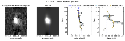
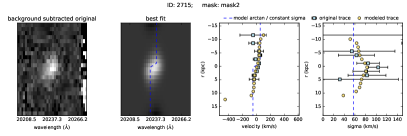
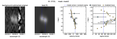
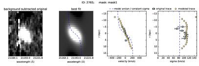
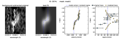
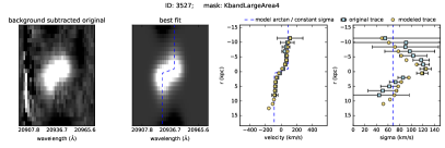
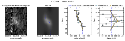
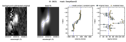
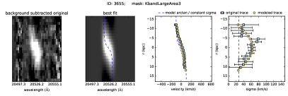
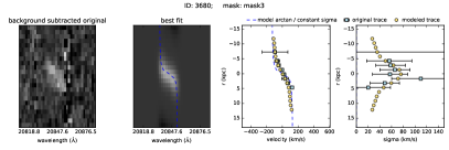
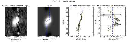
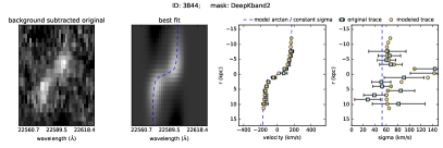
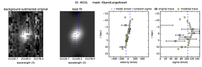
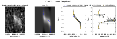
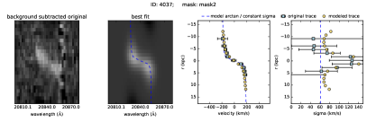
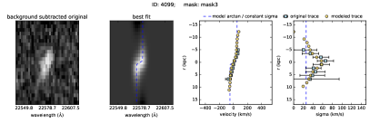
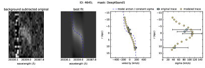
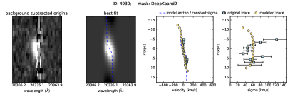
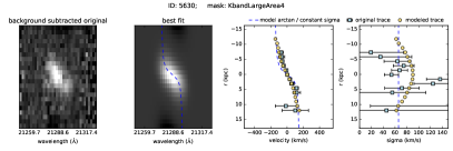
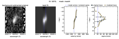
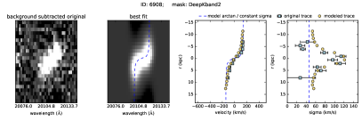
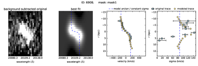
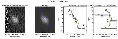
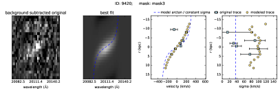
In this Section we present the spectral image stamps and best fits for 24 spectra (Figure 14). In addition to the two-dimensional fits, we derived radial velocity and sigma profiles from gaussian fits to the flux intensity of each row of the spectral image stamp. The center of each gaussian traces the relative blue- or redshift from the center and can be converted to velocity using the kinematic center from the two-dimensional fits. In this way we can also derive the radial velocity dispersion profile, which is not constant due to the seeing (note that for the two-dimensional model we assumed an intrinsic constant velocity dispersion). For each spectrum we repeated this measurement for the modeled images. The errors on the trace were derived from the covariance matrix that was produced by the Python scipy optimize.leastsq algorithm and give an indication of the goodness of the fits to each row.

The radial velocity profile deviates in the center from the intrinsic arctangent, because it was measured on the convolved image. Overall, the original and modeled trace correspond within the uncertainties, indicating an arctangent profile is a reasonable approximation of the velocity curve. These figures further illustrate the advantage of a full two-dimensional analysis: we can accurately reproduce the velocity curves over a large radial range, whereas the trace measured from individual rows can have large uncertainties due to low SNR.

References

- Abraham & van den Bergh (2001) Abraham, R. G., & van den Bergh, S. 2001, Science, 293, 1273
- Alcorn et al. (2016) Alcorn, L. Y., Tran, K.-V. H., Kacprzak, G. G., et al. 2016, ApJ, 825, L2
- Bamford et al. (2006) Bamford, S. P., Aragón-Salamanca, A., & Milvang-Jensen, B. 2006, MNRAS, 366, 308
- Behroozi et al. (2010) Behroozi, P. S., Conroy, C., & Wechsler, R. H. 2010, ApJ, 717, 379
- Bekiaris et al. (2016) Bekiaris, G., Glazebrook, K., Fluke, C. J., & Abraham, R. 2016, MNRAS, 455, 754
- Bell & de Jong (2001) Bell, E. F., & de Jong, R. S. 2001, ApJ, 550, 212
- Bell et al. (2003) Bell, E. F., McIntosh, D. H., Katz, N., & Weinberg, M. D. 2003, ApJS, 149, 289
- Benson (2012) Benson, A. J. 2012, New A, 17, 175
- Brammer et al. (2008) Brammer, G. B., van Dokkum, P. G., & Coppi, P. 2008, ApJ, 686, 1503
- Bruzual & Charlot (2003) Bruzual, G., & Charlot, S. 2003, MNRAS, 344, 1000
- Calzetti et al. (2000) Calzetti, D., Armus, L., Bohlin, R. C., et al. 2000, ApJ, 533, 682
- Chabrier (2003) Chabrier, G. 2003, Publications of the Astronomical Society of the Pacific, 115, 763
- Conroy (2013) Conroy, C. 2013, ARA&A, 51, 393
- Conselice et al. (2005) Conselice, C. J., Bundy, K., Ellis, R. S., et al. 2005, ApJ, 628, 160
- Courteau (1997) Courteau, S. 1997, AJ, 114, 2402
- Cowley et al. (2016) Cowley, M. J., Spitler, L. R., Tran, K.-V. H., et al. 2016, MNRAS, 457, 629
- Cresci et al. (2009) Cresci, G., Hicks, E. K. S., Genzel, R., et al. 2009, ApJ, 697, 115
- Dutton et al. (2011) Dutton, A. A., van den Bosch, F. C., Faber, S. M., et al. 2011, MNRAS, 410, 1660
- Fall & Efstathiou (1980) Fall, S. M., & Efstathiou, G. 1980, MNRAS, 193, 189
- Förster Schreiber et al. (2009) Förster Schreiber, N. M., Genzel, R., Bouché, N., et al. 2009, ApJ, 706, 1364
- Franx & de Zeeuw (1992) Franx, M., & de Zeeuw, T. 1992, ApJ, 392, L47
- Franx et al. (1989) Franx, M., Illingworth, G., & Heckman, T. 1989, AJ, 98, 538
- Franx et al. (2008) Franx, M., van Dokkum, P. G., Schreiber, N. M. F., et al. 2008, ApJ, 688, 770
- Freeman (1970) Freeman, K. C. 1970, ApJ, 160, 811
- Glazebrook (2013) Glazebrook, K. 2013, PASA, 30, 56
- Gnerucci et al. (2011) Gnerucci, A., Marconi, A., Cresci, G., et al. 2011, A&A, 528, A88
- Hammer et al. (2005) Hammer, F., Flores, H., Elbaz, D., et al. 2005, A&A, 430, 115
- Harrison et al. (2017) Harrison, C. M., Johnson, H. L., Swinbank, A. M., et al. 2017, ArXiv e-prints, arXiv:1701.05561
- Haynes & Giovanelli (1984) Haynes, M. P., & Giovanelli, R. 1984, AJ, 89, 758
- Hung et al. (2015) Hung, C.-L., Rich, J. A., Yuan, T., et al. 2015, ApJ, 803, 62
- Kassin et al. (2007) Kassin, S. A., Weiner, B. J., Faber, S. M., et al. 2007, ApJ, 660, L35
- Kassin et al. (2012) —. 2012, ApJ, 758, 106
- Kelly (2007) Kelly, B. C. 2007, ApJ, 665, 1489
- Kriek et al. (2009) Kriek, M., van Dokkum, P. G., Labbé, I., et al. 2009, ApJ, 700, 221
- Kriek et al. (2015) Kriek, M., Shapley, A. E., Reddy, N. A., et al. 2015, ApJS, 218, 15
- Kroupa (2001) Kroupa, P. 2001, MNRAS, 322, 231
- Lawrence et al. (2007) Lawrence, A., Warren, S. J., Almaini, O., et al. 2007, MNRAS, 379, 1599
- McLean et al. (2010) McLean, I. S., Steidel, C. C., Epps, H., et al. 2010, in Society of Photo-Optical Instrumentation Engineers (SPIE) Conference Series, Vol. 7735, Society of Photo-Optical Instrumentation Engineers (SPIE) Conference Series, 1
- Miller et al. (2011) Miller, S. H., Bundy, K., Sullivan, M., Ellis, R. S., & Treu, T. 2011, ApJ, 741, 115
- Miller et al. (2012) Miller, S. H., Ellis, R. S., Sullivan, M., et al. 2012, ApJ, 753, 74
- Mo et al. (1998) Mo, H. J., Mao, S., & White, S. D. M. 1998, MNRAS, 295, 319
- Mortlock et al. (2013) Mortlock, A., Conselice, C. J., Hartley, W. G., et al. 2013, MNRAS, 433, 1185
- Nanayakkara et al. (2016) Nanayakkara, T., Glazebrook, K., Kacprzak, G. G., et al. 2016, ApJ, 828, 21
- Navarro et al. (1997) Navarro, J. F., Frenk, C. S., & White, S. D. M. 1997, ApJ, 490, 493
- Papovich et al. (2010) Papovich, C., Momcheva, I., Willmer, C. N. A., et al. 2010, ApJ, 716, 1503
- Papovich et al. (2015) Papovich, C., Labbé, I., Quadri, R., et al. 2015, ApJ, 803, 26
- Peng et al. (2010) Peng, C. Y., Ho, L. C., Impey, C. D., & Rix, H.-W. 2010, AJ, 139, 2097
- Persson et al. (2013) Persson, S. E., Murphy, D. C., Smee, S., et al. 2013, PASP, 125, 654
- Pizagno et al. (2005) Pizagno, J., Prada, F., Weinberg, D. H., et al. 2005, ApJ, 633, 844
- Pizagno et al. (2007) —. 2007, AJ, 134, 945
- Price et al. (2015) Price, S. H., Kriek, M., Shapley, A. E., et al. 2015, ArXiv e-prints, arXiv:1511.03272
- Puech et al. (2008) Puech, M., Flores, H., Hammer, F., et al. 2008, A&A, 484, 173
- Reddy et al. (2005) Reddy, N. A., Erb, D. K., Steidel, C. C., et al. 2005, ApJ, 633, 748
- Reyes et al. (2011) Reyes, R., Mandelbaum, R., Gunn, J. E., Pizagno, J., & Lackner, C. N. 2011, MNRAS, 417, 2347
- Sales et al. (2010) Sales, L. V., Navarro, J. F., Schaye, J., et al. 2010, MNRAS, 409, 1541
- Salpeter (1955) Salpeter, E. E. 1955, ApJ, 121, 161
- Scoville et al. (2007) Scoville, N., Aussel, H., Brusa, M., et al. 2007, ApJS, 172, 1
- Sersic (1968) Sersic, J. L. 1968, Atlas de galaxias australes
- Simons et al. (2016) Simons, R. C., Kassin, S. A., Trump, J. R., et al. 2016, ApJ, 830, 14
- Skelton et al. (2014) Skelton, R. E., Whitaker, K. E., Momcheva, I. G., et al. 2014, ArXiv e-prints, arXiv:1403.3689
- Somerville et al. (2008) Somerville, R. S., Barden, M., Rix, H.-W., et al. 2008, ApJ, 672, 776
- Spitler et al. (2012) Spitler, L. R., Labbé, I., Glazebrook, K., et al. 2012, ApJ, 748, L21
- Spitler et al. (2014) Spitler, L. R., Straatman, C. M. S., Labbé, I., et al. 2014, ApJ, 787, L36
- Steidel et al. (2014) Steidel, C. C., Rudie, G. C., Strom, A. L., et al. 2014, ApJ, 795, 165
- Straatman et al. (2015) Straatman, C. M. S., Labbé, I., Spitler, L. R., et al. 2015, ApJ, 808, L29
- Straatman et al. (2016) Straatman, C. M. S., Spitler, L. R., Quadri, R. F., et al. 2016, ArXiv e-prints, arXiv:1608.07579
- Tiley et al. (2016) Tiley, A. L., Stott, J. P., Swinbank, A. M., et al. 2016, MNRAS, 460, 103
- Tomczak et al. (2014) Tomczak, A. R., Quadri, R. F., Tran, K.-V. H., et al. 2014, ApJ, 783, 85
- Tomczak et al. (2015) —. 2015, ArXiv e-prints, arXiv:1510.06072
- Tully & Fisher (1977) Tully, R. B., & Fisher, J. R. 1977, A&A, 54, 661
- van der Wel et al. (2012) van der Wel, A., Bell, E. F., Häussler, B., et al. 2012, ApJS, 203, 24
- van der Wel et al. (2014a) van der Wel, A., Franx, M., van Dokkum, P. G., et al. 2014a, ApJ, 788, 28
- van der Wel et al. (2014b) van der Wel, A., Chang, Y.-Y., Bell, E. F., et al. 2014b, ApJ, 792, L6
- van Dokkum & Franx (2001) van Dokkum, P. G., & Franx, M. 2001, ApJ, 553, 90
- Vergani et al. (2012) Vergani, D., Epinat, B., Contini, T., et al. 2012, A&A, 546, A118
- Weiner et al. (2006a) Weiner, B. J., Willmer, C. N. A., Faber, S. M., et al. 2006a, ApJ, 653, 1027
- Weiner et al. (2006b) —. 2006b, ApJ, 653, 1049
- Whitaker et al. (2012) Whitaker, K. E., van Dokkum, P. G., Brammer, G., & Franx, M. 2012, ApJ, 754, L29
- Willick (1999) Willick, J. A. 1999, ApJ, 516, 47
- Yuan et al. (2014) Yuan, T., Nanayakkara, T., Kacprzak, G. G., et al. 2014, ApJ, 795, L20