Numerical stochastic homogenization by quasilocal effective diffusion tensors

Abstract

This paper proposes a numerical upscaling procedure for elliptic boundary value problems with diffusion tensors that vary randomly on small scales. The method compresses the random partial differential operator to an effective quasilocal deterministic operator that represents the expected solution on a coarse scale of interest. Error estimates consisting of a priori and a posteriori terms are provided that allow one to quantify the impact of uncertainty in the diffusion coefficient on the expected effective response of the process.

Keywords numerical homogenization, multiscale method, upscaling, a priori error estimates, a posteriori error estimates, uncertainty, modeling error estimate, model reduction

AMS subject classification 35R60, 65N12, 65N15, 65N30, 73B27, 74Q05

1 Introduction

Homogenization is a tool of mathematical modeling to identify reduced descriptions of the macroscopic response of multiscale models. In the context of the prototypical elliptic model problem

$$-\operatorname{div}(\mathbf{A}_{\varepsilon}\nabla\mathbf{u}_{\varepsilon})=f$$

microscopic features on some characteristic length scale $\varepsilon$ are encoded in the diffusion coefficient $\mathbf{A}_{\varepsilon}$ and homogenization studies the limit as $\varepsilon$ tends to zero. It turns out that suitable limits represented by the so-called effective or homogenized coefficient exist in fairly general settings in the framework of $G$-, $H$-, or two-scale convergence [Spa68, DG75, MT78, Ngu89, All92]. However, the effective coefficient is rarely given explicitly and even its implicit representation based on cell problems usually requires structural assumptions on the sequence of coefficients $\mathbf{A}_{\varepsilon}$ such as local periodicity and scale separation [BLP78, JKO94]. Moreover, in many interesting applications such as geophysics and material sciences where $\mathbf{A}_{\varepsilon}$ represents porosity or permeability, complete explicit knowledge of the coefficient is unlikely. The coefficient is rather the result of measurements that underlie errors or it is the result of singular measurements combined with inverse modeling. In any case, it is very likely that there is uncertainty in the data $\mathbf{A}_{\varepsilon}$. The question is how this uncertainty on the fine scale $\varepsilon$ changes the expected macroscopic response of the process. For works on analytical stochastic homogenization we refer to the classical works [Koz79, PV81, Yur86] and the recent approaches [BP04], [GO11, GO12, GNO14, GNO15, GO15, DGO16, GO17], and [AS16, AKM17]. Computational methods in stochastic homogenization comprise [EMZ05, CS08, GMP10, BJ11, LLT14, JMSDO14, ZCH15] and the review article [ACL⁺12]. However, important practical and theoretical questions remain open. Among them are the truncation of cell problems (see [Glo12a, Glo12b, GH16] for recent progress on this aspect), the role of discretization on the different scales and its interaction with the homogenization process as well as the incorporation of macroscopic boundary conditions.

This paper addresses all these issues to some extent. It provides a method to compute effective, deterministic models such that the corresponding discrete solution is close to $\mathbb{E}[\mathbf{u}_{\varepsilon}]$, the expected value of $\mathbf{u}_{\varepsilon}$; closeness is meant in the $L^{2}$ sense, so that a meaningful approximation is achieved on some coarse scale of interest $H$ (observation scale) which is typically linked to some triangulation $\mathcal{T}_{H}$ of mesh-size $H$. The numerical method is based on the multiscale approach of [MP14], sometimes referred to as Localized Orthogonal Decomposition (LOD), that was developed for the deterministic case (see also [HP13, GP15, Pet16, KPY18]). The basis functions therein are constructed by local corrections (generally different from those of analytical homogenization theory) that solve some elliptic fine-scale problem on localized patch domains. Their supports are determined by oversampling lengths $H\lvert\log H\rvert$, where $H$ denotes the mesh-size of a finite element triangulation $\mathcal{T}_{H}$ on the observation scale. This choice of oversampling is justified by the exponential decay of the correctors away from their source [MP14, HP13, KY16, KPY18]. The method leads to quasi-optimal a priori error estimates and can dispense with any assumptions on scale separation.

The recent work [GP17] gives a re-interpretation of the method from [MP14] as a quasilocal discrete integral operator for the deterministic case. In a further compression step, this representation allows to extract a piecewise constant diffusion tensor. An application of this procedure for any atom $\omega$ in the probability space leads to an integral operator $\mathcal{A}_{H}$ (depending on the stochastic variable) and a corresponding piecewise constant random field $\mathbf{A}_{H}$ on the scale $H$. It turns out that this viewpoint is useful in the stochastic setting because it allows to average in the stochastic variable over effective coefficients rather than over multiscale basis functions and to thereby characterize the resulting effective model in terms of quasi-local coefficients and even deterministic PDEs. The averages are given by $\bar{\mathcal{A}}_{H}:=\mathbb{E}[\mathcal{A}_{H}]$ and $\bar{A}_{H}:=\mathbb{E}[\mathbf{A}_{H}]$ and constitute deterministic models which we refer to as quasi-local ($\bar{\mathcal{A}}_{H}$) and local ($\bar{A}_{H}$), respectively. The proposed method covers the case of bounded polytopes, which appears still open in analytical stochastic homogenization. The method itself can dispense with any a priori information on the coefficient. The validity of the discrete model is assessed via an a posteriori model error estimator. In order to make the computation of $\bar{\mathcal{A}}_{H}$ and $\bar{A}_{H}$ feasible, one can exploit the structure (if available) of the stochastic coefficient $\mathbf{A}_{\varepsilon}$ as well as the underlying mesh. Provided the dependence of the stochastic variable has a suitable structure, sampling procedures for $\mathbf{A}_{H}$ are purely local and allow to restrict the computations to reference configurations.

We provide error estimates for the expected error in the $L^{2}$ norm as well as the $L^{2}$ norm of the expected error. The upper bounds are combined from a priori terms and a posteriori terms. The latter contributions are determined by the statistics of the local fluctuations of the upscaled coefficient. Numerical evidence for an uncorrelated model coefficient suggests that the error estimator is not the dominant part in the error, as long as the usual scaling $H\approx(\varepsilon/H)^{d/2}$ from the central limit theorem (CLT) is satisfied.

The structure of this article is as follows. Section 2 introduces the general model problem, relevant notation for data structures and function spaces, and gives an example of a possible model situation. Section 3 presents the upscaling procedure. Section 4 provides error estimates in the $L^{2}$ norm. Numerical experiments are presented in Section 5. The comments of Section 6 conclude the paper.

Standard notation on Lebesgue and Sobolev spaces applies throughout this paper. The notation $a\lesssim b$ abbreviates $a\leq Cb$ for some constant $C$ that is independent of the mesh-size, but may depend on the contrast of the coefficient $\mathbf{A}$; $a\approx b$ abbreviates $a\lesssim b\lesssim a$. The symmetric part of a quadratic matrix $M$ is denoted by $\operatorname{sym}(M)$.

2 Model problem and notation

This section describes the model problem and some notation on finite element spaces. Finally, an example of a possible model situation is discussed.

2.1 Model problem

Let $(\Omega,\mathcal{F},\mathbb{P})$ be a probability space with set of events $\Omega$, $\sigma$-algebra $\mathcal{F}\subseteq 2^{\Omega}$ and probability measure $\mathbb{P}$. The expectation operator is denoted by $\mathbb{E}$. Let $D\subseteq\mathbb{R}^{d}$ for $d\in\{1,2,3\}$ be a bounded Lipschitz polytope. The set of admissible coefficients reads

$$\mathcal{M}(D,\alpha,\beta)=\left\{\begin{aligned} A\in L^{\infty}(D;\mathbb{R}^{d\times d}_{\mathrm{sym}})&\text{ s.t. }\,\alpha|\xi|^{2}\leq(A(x)\xi)\cdot\xi\leq\beta|\xi|^{2}\\ &\text{for a.e. }x\in D\text{ and all }\xi\in\mathbb{R}^{d}\end{aligned}\right\}.$$ (2.1)

Here, $\mathbb{R}^{d\times d}_{\mathrm{sym}}$ denotes the set of symmetric $d\times d$ matrices. Note that the elements of $A\in\mathcal{M}(D,\alpha,\beta)$ are fairly free to vary within the bounds $\alpha$ and $\beta$ and that we do not assume any frequencies of variation or smoothness.

Let $\mathbf{A}$ be an $\mathcal{M}(D,\alpha,\beta)$-valued, pointwise symmetric random field with $\beta>\alpha>0$ and let, for the sake of readability, $f\in L^{2}(D)$ be deterministic. Throughout this article we suppress the characteristic length scale $\varepsilon$ of the diffusion coefficient in the notation and write $\mathbf{A}$ instead of $\mathbf{A}_{\varepsilon}$. Consider the model problem

$$\left\{\begin{aligned} -\operatorname{div}(\mathbf{A}(\omega)(x)\nabla\mathbf{u}(\omega)(x))&=f(x),&x\in D\\ \mathbf{u}(\omega)(x)&=0,&x\in\partial D\end{aligned}\right\}\quad\text{for almost all }\omega\in\Omega.$$ (2.2)

Denote the energy space by $V:=H^{1}_{0}(D)$. The weak formulation of (2.2) seeks a $V$-valued random field $\mathbf{u}$ such that for almost all $\omega\in\Omega$

$$\int_{D}(\mathbf{A}(\omega)(x)\nabla\mathbf{u}(\omega))(x)\cdot\nabla v(x)\,dx=\int_{D}f(x)v(x)\,dx\quad\text{for all }v\in V.$$ (2.3)

The reformulation of this problem in the Hilbert space $L^{2}(\Omega;V)$ of $V$-valued random fields with finite second moments leads to a coercive variational problem that seeks $\mathbf{u}\in L^{2}(\Omega;V)$ such that

$$\int_{\Omega}\int_{D}(\mathbf{A}(\omega)\nabla\mathbf{u}(\omega)(x))\cdot\nabla\mathbf{v}(\omega)(x)\,dx\,d\mathbb{P}(\omega)=\int_{\Omega}\int_{D}f(x)\mathbf{v}(\omega)(x)\,dx\,d\mathbb{P}(\omega)$$

holds for all $\mathbf{v}\in L^{2}(\Omega;V)$. It is easily checked that this is a well-posed problem in the sense of the Lax-Milgram theorem with a coercive and bounded bilinear form

$$a:L^{2}(\Omega;V)\times L^{2}(\Omega;V) \rightarrow\mathbb{R},$$

$$(\mathbf{u},\mathbf{v}) \mapsto\int_{\Omega}\int_{D}(\mathbf{A}(\omega)(x)\nabla\mathbf{u}(\omega)(x))\cdot\nabla\mathbf{v}(\omega)(x)\,dx\,d\mathbb{P}(\omega)$$

and a bounded linear functional $F$ on $L^{2}(\Omega;V)$ given by

$$\mathbf{v}\mapsto\int_{\Omega}\int_{D}f(x)\mathbf{v}(\omega)(x)\,dx\,d\mathbb{P}(\omega).$$

This shows that, for any $f\in L^{2}(D)$, there exists a unique solution $\mathbf{u}\in L^{2}(\Omega;V)$ with

$$\|\nabla\mathbf{u}\|_{L^{2}(\Omega;V)}:=\left(\int_{\Omega}\int_{D}|\nabla(\mathbf{u}(\omega))(x)|^{2}\,dx\,d\mathbb{P}(\omega)\right)^{1/2}\leq C(D)\alpha^{-1}\|f\|_{L^{2}(D)}.$$

Though it would be possible, we disregard the possibility of more general $f\in H^{-1}(D)$ or uncertainty in the right-hand side $f$ in this article.

Remark 1.

The parameter $\varepsilon$ refers to some scale that resolves the stochastic data. We do not assume any particular structure; the coefficient $\mathbf{A}=\mathbf{A}_{\varepsilon}$ is not necessarily part of some ergodic sequence. Our viewpoint is that of coarsening/reducing the given model on the fixed scale $\varepsilon$ to the observation scale $H$ rather than that of the asymptotics for small $\varepsilon$.

2.2 Finite element spaces

Let $\mathcal{T}_{H}$ be a quasi-uniform regular simplicial triangulation of $D$ and let $V_{H}$ denote the standard $P_{1}$ finite element space, that is, the subspace of $V$ consisting of piecewise first-order polynomials. Given any subdomain $S\subseteq\overline{D}$, define its neighbourhood via

$$\mathsf{N}(S):=\operatorname{int}\Big{(}\cup\{T\in\mathcal{T}_{H}\,:\,T\cap\overline{S}\neq\emptyset\}\Big{)}.$$

Furthermore, we introduce for any $m\geq 2$ the patch extensions

$$\mathsf{N}^{1}(S):=\mathsf{N}(S)\qquad\text{and}\qquad\mathsf{N}^{m}(S):=\mathsf{N}(\mathsf{N}^{m-1}(S)).$$

Throughout this paper, we assume that the coarse-scale mesh $\mathcal{T}_{H}$ is quasi-uniform. The global mesh-size reads $H:=\max\{\operatorname{diam}(T):T\in\mathcal{T}_{H}\}$. Note that the shape-regularity implies that there is a uniform bound $C(m)$ on the number of elements in the $m$th-order patch, $\operatorname{card}\{K\in\mathcal{T}_{H}\,:\,K\subseteq\overline{\mathsf{N}^{m}(T)}\}\leq C(m)$ for all ${T\in\mathcal{T}_{H}}$. The constant $C(m)$ depends polynomially on $m$. The set of interior $(d-1)$-dimensional hyper-faces of $\mathcal{T}_{H}$ is denoted by $\mathcal{F}_{H}$. For a piecewise continuous function $\varphi$, we denote the jump across an interior edge by $[\varphi]_{F}$, where the index $F$ will be sometimes omitted for brevity. The space of piecewise constant functions (resp. $d\times d$ matrix fields) is denoted by $P_{0}(\mathcal{T}_{H})$ (resp. $P_{0}(\mathcal{T}_{H};\mathbb{R}^{d\times d})$).

Let $I_{H}:V\to V_{H}$ be a surjective quasi-interpolation operator that acts as an $H^{1}$-stable and $L^{2}$-stable quasi-local projection in the sense that $I_{H}\circ I_{H}=I_{H}$ and that for any $T\in\mathcal{T}_{H}$ and all $v\in V$ there holds

$$H^{-1}\|v-I_{H}v\|_{L^{2}(T)}+\|\nabla I_{H}v\|_{L^{2}(T)} \leq C_{I_{H}}\|\nabla v\|_{L^{2}(\mathsf{N}(T))}$$

$$\|I_{H}v\|_{L^{2}(T)} \leq C_{I_{H}}\|v\|_{L^{2}(\mathsf{N}(T))}.$$

Since $I_{H}$ is a stable projection from $V$ to $V_{H}$, any $v\in V$ is quasi-optimally approximated by $I_{H}v$ in the $L^{2}(D)$ norm as well as in the $H^{1}(D)$ norm. One possible choice is to define $I_{H}:=I^{\mathit{c}}_{H}\circ\Pi_{H}$, where $\Pi_{H}$ is the $L^{2}(D)$-orthogonal projection onto the space $P_{1}(\mathcal{T}_{H})$ of piecewise affine (possibly discontinuous) functions and $I^{\mathit{c}}_{H}$ is the averaging operator that maps $P_{1}(\mathcal{T}_{H})$ to $V_{H}$ by assigning to each free vertex the arithmetic mean of the corresponding function values of the neighbouring cells, that is, for any $v\in P_{1}(\mathcal{T}_{H})$ and any free vertex $z$ of $\mathcal{T}_{H}$,

$$(I^{\mathit{c}}_{H}(v))(z)=\sum_{\begin{subarray}{c}T\in\mathcal{T}_{H}\\ \text{with }z\in T\end{subarray}}v|_{T}(z)\bigg{/}\operatorname{card}\{K\in\mathcal{T}_{H}\,:\,z\in K\}.$$

This choice of $I_{H}$ is employed in our numerical experiments.

2.3 Discrete stochastic setting

In this subsection we briefly describe one possible discrete stochastic setting where the uncertainty is encoded by a triangulation $\mathcal{T}_{\varepsilon}$. Although it is not the most general coefficient that can be treated with the methods described below, it appears as a natural model situation in a multiscale setting and will therefore be utilized in the numerical experiments from Section 5.

We assume that the triangulation $\mathcal{T}_{\varepsilon}$ describing the multiscale structure of $\mathbf{A}$ is a uniform refinement of the triangulation $\mathcal{T}_{H}$ on the observation scale. Let $\mathcal{T}_{\varepsilon}$ denote a uniform triangulation. The probability space reads

$$\Omega=\prod_{T\in\mathcal{T}_{\varepsilon}}[\alpha,\beta]=[\alpha,\beta]^{\operatorname{card}\mathcal{T}_{\varepsilon}}.$$

Each $\omega=(\omega_{T})_{T\in\mathcal{T}_{\varepsilon}}\in\Omega$ can be identified with a scalar $\mathcal{T}_{\varepsilon}$-piecewise constant function $\iota\omega$ over $D$ with $\iota\omega|_{T}=\omega_{T}$ for any $T\in\mathcal{T}_{\varepsilon}$. The scalar random diffusion coefficient $\mathbf{A}=\mathbf{A}_{\varepsilon}$ is a random variable $\mathbf{A}\in L^{2}(\Omega;\mathcal{M}(D,\alpha,\beta))$. The values are piecewise constant in space, that is

$$\mathbf{A}(\bullet,\omega)=\iota\omega\in P_{0}(\mathcal{T}_{\varepsilon})\quad\text{for any }\omega\in\Omega.$$

Of course, similar settings are possible for tensor-valued diffusion coefficients.

3 Upscaling method

This section describes the proposed upscaling methods.

3.1 Upscaling with a quasi-local effective model

This subsection describes the computation of a quasi-local effective coefficient. The underlying model does not correspond to a PDE but rather to a discrete integral operator on finite element spaces. The method is very flexible in that it is not restricted to (quasi-)periodic situations and is able to include boundary conditions.

The upscaling procedure presented here is based on the multiscale approach of [MP14, HP13]. For the deterministic case, it was shown in [GP17] that a variant of those methods corresponds to a finite element system with a quasilocal discrete integral operator. Its construction for the stochastic setting is described in the following.

Let $W:=\operatorname{ker}I_{H}\subseteq V$ denote the kernel of $I_{H}$. The space $W$ is referred to as fine-scale space. For any element $T\in\mathcal{T}_{H}$ define the extended element patch $D_{T}:=\mathsf{N}^{\ell}(T)$ of order $\ell$. The nonnegative integer $\ell$ is referred to as the oversampling parameter. As a crucial parameter in the design of the multiscale method, it is inherent to all quantities in the upscaled model. The parameter will always be chosen $\ell\approx\lvert\log H\rvert$. For better readability we will suppress the explicit dependence on $\ell$ whenever there is no risk of confusion, but stress the fact that quantities like $\mathbf{q}_{T,j}$ $\mathcal{C}$, $\mathcal{A}_{H}$, etc. defined below should be understood as $\mathbf{q}_{T,j}^{(\ell)}$ $\mathcal{C}^{(\ell)}$, $\mathcal{A}_{H}^{(\ell)}$.

Let $W_{D_{T}}\subseteq W$ denote the space of functions from $W$ that vanish outside $D_{T}$. For any $T\in\mathcal{T}_{H}$, any $j\in\{1,\dots,d\}$, and any $v_{H}\in V_{H}$, the function $\mathbf{q}_{T,j}\in L^{2}(\Omega;W_{D_{T}})$ solves

$$\int_{D_{T}}\nabla w\cdot(\mathbf{A}\nabla\mathbf{q}_{T,j})\,dx=\int_{T}\nabla w\cdot(\mathbf{A}e_{j})\,dx\quad\text{for all }w\in W_{D_{T}}.$$ (3.1)

Here $e_{j}$ ($j=1,\dots,d$) is the $j$th Cartesian unit vector. The functions $\mathbf{q}_{T,j}$ are called element correctors. We emphasize that the element correctors $\mathbf{q}_{T,j}$ are $W_{D_{T}}$-valued random variables. Given $v_{H}\in V_{H}$, we define the corrector $\mathcal{C}v_{H}\in L^{2}(\Omega;W)$ by

$$\mathcal{C}v_{H}=\sum_{T\in\mathcal{T}_{H}}\sum_{j=1}^{d}(\partial_{j}v_{H}|_{T})\mathbf{q}_{T,j}.$$ (3.2)

Again, the operator $\mathcal{C}$ depends on the uncertainty parameter $\omega$. Define the piecewise constant matrix field $\mathcal{A}_{H}\in L^{2}(\Omega;P_{0}(\mathcal{T}_{H}\times\mathcal{T}_{H};\mathbb{R}^{d\times d}))$ over $\mathcal{T}_{H}\times\mathcal{T}_{H}$, for $T,K\in\mathcal{T}_{H}$ by

$$(\mathcal{A}_{H}|_{T,K})_{jk}:=\frac{1}{|T|\,|K|}\left(\delta_{T,K}\int_{T}\mathbf{A}_{jk}\,dx-e_{j}\cdot\int_{K}\mathbf{A}\nabla\mathbf{q}_{T,k}\,dx\right)$$ (3.3)

($j,k=1,\dots,d$) where $\delta$ is the Kronecker symbol. The bilinear form $\mathfrak{a}:V\times V\to L^{2}(\Omega;\mathbb{R})$ is given by

$$\mathfrak{a}(v_{H},z_{H}):=\int_{D}\int_{D}\nabla v_{H}(x)\cdot(\mathcal{A}_{H}(x,y)\nabla z_{H}(y))\,dy\,dx\quad\text{for any }v_{H},z_{H}\in V_{H}.$$

As pointed out in [GP17], there holds for all finite element functions $v_{H},z_{H}\in V_{H}$ that

$$\int_{D}\nabla v_{H}\cdot(\mathbf{A}\nabla(1-\mathcal{C})z_{H})\,dx=\mathfrak{a}(v_{H},z_{H}).$$ (3.4)

Remark 2.

The nonlocal operator $\mathcal{A}_{H}$ is sparse in the sense that $\mathcal{A}_{H}|_{T,K}$ equals zero whenever $\operatorname{dist}(T,K)\gtrsim\ell H$ for $T,K\in\mathcal{T}_{H}$. It is therefore referred to as quasilocal.

Remark 3.

The left-hand side of (3.4) corresponds to a Petrov-Galerkin method with finite element trial functions and modified test functions. Such multiscale basis functions were proposed in [MP14]. For averaging procedures over the stochastic variable, it will turn out that the representation from the right-hand side of (3.4) is preferable. In other words, we average the nonlocal integral kernel rather than multiscale basis functions. Therefore we employ the variant from [GP17] where in the discretization the right-hand side of the PDE is only tested with standard finite element functions, while in the original method [MP14] the right hand side was tested with multiscale test functions. Those would be random variables in our case.

If the oversampling parameter $\ell$ is chosen in the order of magnitude $\mathcal{O}(\lvert\log H\rvert)$, it can be shown (see e.g., [GP17, proof of Prop. 6]) that the bilinear form $\mathfrak{a}$ is coercive and continuous

$$\|\nabla v_{H}\|_{L^{2}(D)}\lesssim\mathfrak{a}(v_{H},v_{H})\lesssim\|\nabla v_{H}\|_{L^{2}(D)}\quad\text{for all }v_{H}\in V_{H}$$ (3.5)

for any $\omega\in\Omega$. Hence, there exists a unique solution $\mathbf{u}_{H}\in L^{2}(\Omega;V_{H})$ to

$$\mathfrak{a}(\mathbf{u}_{H},v_{H})=(f,v_{H})_{L^{2}(D)}\quad\text{for all }v_{H}\in V_{H}.$$ (3.6)

Is is known that the method of [MP14] produces quasi-optimal results for every fixed $\omega$. More precisely, for the variant considered here, [GP17, Prop. 1] states

$$\frac{\|\mathbf{u}(\omega)-\mathbf{u}_{H}(\omega)\|_{L^{2}(D)}}{\|f\|_{L^{2}(D)}}\lesssim H^{2}+\bm{\mathrm{wcba}}(\mathbf{A}(\omega),\mathcal{T}_{H}).$$ (3.7)

The term $\bm{\mathrm{wcba}}(\mathbf{A}(\omega),\mathcal{T}_{H}))$ denotes the worst-case best-approximation error

$$\bm{\mathrm{wcba}}(\mathbf{A}(\omega),\mathcal{T}_{H}):=\sup_{g\in L^{2}(D)\setminus\{0\}}\inf_{v_{H}\in V_{H}}\frac{\|u(g,\mathbf{A}(\omega))-v_{H}\|_{L^{2}(D)}}{\|g\|_{L^{2}(D)}}$$ (3.8)

where for $g\in L^{2}(D)$, $u(g,\mathbf{A}(\omega))\in V$ solves the deterministic model problem with diffusion coefficient $\mathbf{A}(\omega)$ and right-hand side $g$. In particular, the right-hand side of (3.7) is always controlled by $H\|f\|_{L^{2}(D)}$.

The approximation by a deterministic model is based on the averaged integral kernel $\bar{\mathcal{A}}_{H}:=\mathbb{E}[\mathcal{A}_{H}]$. In view of (3.3), the values of the piecewise constant integral kernel $\bar{\mathcal{A}}_{H}$ on two simplices $T,K\in\mathcal{T}_{H}$ are given by

$$(\bar{\mathcal{A}}_{H}|_{T,K})_{jk}=\frac{1}{|T|\,|K|}\left(\delta_{T,K}\int_{T}\mathbb{E}[\mathbf{A}_{jk}]\,dx-e_{j}\cdot\int_{K}\mathbb{E}[\mathbf{A}\nabla\mathbf{q}_{T,k}]\,dx\right).$$ (3.9)

The corresponding bilinear form $\bar{\mathfrak{a}}(\cdot,\cdot)$ given by

$$\bar{\mathfrak{a}}(v_{H},z_{H}):=\int_{D}\int_{D}\nabla v_{H}(x)\cdot(\bar{\mathcal{A}}_{H}(x,y)\nabla z_{H}(y))\,dy\,dx\quad\text{for any }v_{H},z_{H}\in V_{H}.$$

The discrete solution $u_{H}\in V_{H}$ to the quasilocal deterministic model is given by

$$\bar{\mathfrak{a}}(u_{H},v_{H})=(f,v_{H})_{L^{2}(D)}\quad\text{for all }v_{H}\in V_{H}.$$ (3.10)

Remark 4.

In practice, the stochastic averages in (3.9) are approximated through sampling procedures. This is indeed feasible because for some $T\in\mathcal{T}_{H}$ and $\omega\in\Omega$, the computation of $\mathcal{A}_{H}|_{T,K}(\omega)$ for any $K\in\mathcal{T}_{H}$ corresponds to the solution of problem (3.1), which is posed on the quasilocal neighbourhood $D_{T}$ of $T$.

3.2 Compression to a local deterministic coefficient

Given the quasilocal upscaled coefficient, one may ask whether there exists a suitable approximation by a PDE model. In order to provide a fully local model, a further compression step is introduced [GP17]. The nonlocal bilinear form $\mathfrak{a}(\cdot,\cdot)$ is approximated by a quadrature-like procedure as follows. Define the piecewise constant coefficient

$$\mathbf{A}_{H}\in L^{2}(\Omega;P_{0}(\mathcal{T}_{H};\mathbb{R}^{d\times d}))\quad\text{by}\quad\mathbf{A}_{H}|_{T}:=\sum_{K\in\mathcal{T}_{H}}|K|\,\mathcal{A}_{H}|_{T,K}.$$

For fixed $\omega\in\Omega$, the tensor field $\mathbf{A}_{H}(\omega)$ is the local effective diffusion coefficient of [GP17] on the mesh $\mathcal{T}_{H}$. In particular, $\mathbf{A}_{H}$ still depends on $x$ and $\omega$. We define the deterministic diffusion tensor by

$$\bar{A}_{H}:=\mathbb{E}[\mathbf{A}_{H}].$$

By linearity of the expectation operator, $\bar{A}_{H}$ is equivalently obtained by compressing the averaged operator $\bar{\mathcal{A}}_{H}$.

It is not guaranteed a priori that $\bar{A}_{H}$ is uniformly positive definite. In what follows we therefore assume that $\bar{A}_{H}\in\mathcal{M}(D,\alpha/2,2\beta)$. This condition can be checked a posteriori. We denote by $\tilde{u}_{H}\in V_{H}$ the solution to the following finite element system

$$\int_{D}\nabla\tilde{u}_{H}\cdot(\bar{A}_{H}\nabla v_{H})\,dx=(f,v_{H})_{L^{2}(D)}\quad\text{for all }v_{H}\in V_{H}.$$ (3.11)

This effective equation is the discretization of a PDE. As described in Subsection 4.2, the coefficient $\bar{A}_{H}$ can be regularized to some $\bar{A}_{H}^{\mathit{reg}}$ that leads to comparable accuracy.

4 Error analysis

This section provides $L^{2}$ error estimates for the upscaling schemes. The estimates combine a priori and a posteriori terms. The measure for quantifying the error is the $L^{2}(\Omega;L^{2}(D))$ norm, denoted by

$$|||\mathbf{v}|||:=\sqrt{\mathbb{E}[\|\mathbf{v}\|_{L^{2}(D)}^{2}]}.$$

We will also provide error estimates for the $L^{2}$ norm of the expected error.

4.1 Error estimate for the quasilocal method

Definition 5 (model error estimator).

For any $T\in\mathcal{T}_{H}$, denote

$$X(T):=\max_{\begin{subarray}{c}K\in\mathcal{T}_{H}\\ K\cap\mathsf{N}^{\ell}(T)\neq\emptyset\end{subarray}}\lvert T\rvert\,\Big{\lvert}\mathcal{A}_{H}|_{T,K}-\bar{\mathcal{A}}_{H}|_{T,K}\Big{\rvert}.$$

The model error estimator $\gamma$ is defined by

$$\gamma:=\max_{T\in\mathcal{T}_{H}}\Big{(}\sqrt{\mathbb{E}[X(T)^{2}]}\Big{)}\Bigg{/}\Big{(}\max_{T\in\mathcal{T}_{H}}\max_{K\in\mathcal{T}_{H}}\mathbb{E}[\big{\lvert}\bar{\mathcal{A}}_{H}|_{T,K}\big{\rvert}]\Big{)}.$$

Remark 6 (normalization of $\gamma$).

Throughout the analysis of this paper, the constants hidden in the notation $\lesssim$ may involve the contrast $\beta/\alpha$. We use the scaling of $\gamma$ as in Definition 5.

The random variable $X$ measures local fluctuations of $\mathcal{A}_{H}$. Its expectation determines the model error estimator $\gamma$ that is part of the upper bound in the subsequent error estimate. It is a term to be computed a posteriori.

Remark 7.

Note that we have not assumed any particular structure of the coefficient $\mathbf{A}$. Information on the validity of the discrete model is instead extracted from the a posteriori model error estimator $\gamma$. It is expected that small values of $\gamma$ require a certain scale separation in the stochastic variable in the sense of the CLT scaling. If, for example, $\mathbf{A}$ is i.i.d. over $\mathcal{T}_{\varepsilon}$ (with $\mathcal{T}_{\varepsilon}$ from Subsection 2.3), then the value of $\gamma$ is basically determined by the ratio $(\varepsilon/H)^{d/2}$.

Lemma 8.

Let $\ell\approx\lvert\log H\rvert$. Let $\mathbf{u}_{H}$ solve (3.6) and let $u_{H}$ solve (3.10) with right-hand side $f\in L^{2}(D)$. Then, for $\rho:=\lvert\log H\rvert$,

$$|||\nabla(\mathbf{u}_{H}-u_{H})|||\lesssim\rho^{d}\gamma\|f\|_{L^{2}(D)}$$

for the model error estimator $\gamma$ from Definition 5.

Proof.

Denote $\mathbf{e}_{H}:=\mathbf{u}_{H}-u_{H}$. The coercivity (3.5) of the multiscale bilinear form for any atom $\omega\in\Omega$ and the representation as integral operator reveal

$$\|\nabla\mathbf{e}_{H}\|_{L^{2}(D)}^{2}\lesssim\mathfrak{a}(\mathbf{e}_{H},\mathbf{e}_{H})=\int_{D}\int_{D}\nabla(\mathbf{u}_{H}(x)-u_{H}(x))\cdot(\mathcal{A}_{H}(x,y)\nabla\mathbf{e}_{H}(y))\,dy\,dx.$$

Abbreviate $\mathcal{E}|_{T,K}:=\bar{\mathcal{A}}_{H}|_{T,K}-\mathcal{A}_{H}|_{T,K}$. Adding and subtracting $\bar{\mathcal{A}}_{H}(x,y)$ together with the discrete solution properties of $\mathbf{u}_{H}$ and $u_{H}$ lead to

$$\|\nabla\mathbf{e}_{H}\|_{L^{2}(D)}^{2} \lesssim\int_{D}\int_{D}\nabla u_{H}(x)\cdot(\bar{\mathcal{A}}_{H}(x,y)-(\mathcal{A}_{H}(x,y))\nabla\mathbf{e}_{H}(y))\,dy\,dx$$

$$=\sum_{T\in\mathcal{T}_{H}}\sum_{\begin{subarray}{c}K\in\mathcal{T}_{H}\\ K\cap\mathsf{N}^{\ell}(T)\neq\emptyset\end{subarray}}\lvert T\rvert\lvert K\rvert\;\nabla u_{H}|_{T}\cdot(\mathcal{E}|_{T,K}\nabla\mathbf{e}_{H}|_{K})$$

where it was used that $\nabla u_{H}$ and $\nabla\mathbf{e}_{H}$ are piecewise constant. For any fixed $T\in\mathcal{T}_{H}$, the shape regularity of the mesh and equivalence of norms in the finite-dimensional space $\mathbb{R}^{N}$ with $N=\mathcal{O}(\ell^{d})$ lead to

$$\sum_{\begin{subarray}{c}K\in\mathcal{T}_{H}\\ K\cap\mathsf{N}^{\ell}(T)\neq\emptyset\end{subarray}}\lvert T\rvert\lvert K\rvert\;\nabla u_{H}|_{T}\cdot(\mathcal{E}|_{T,K}\nabla\mathbf{e}_{H}|_{K})$$

$$\qquad\lesssim X(T)\lvert T\rvert^{1/2}\lvert\nabla u_{H}|_{T}\rvert\sum_{\begin{subarray}{c}K\in\mathcal{T}_{H}\\ K\cap\mathsf{N}^{\ell}(T)\neq\emptyset\end{subarray}}\lvert K\rvert^{1/2}\lvert\nabla\mathbf{e}_{H}|_{K}\rvert$$

$$\qquad\lesssim\ell^{d/2}X(T)\|\nabla u_{H}\|_{L^{2}(T)}\|\nabla\mathbf{e}_{H}\|_{L^{2}(\mathsf{N}^{\ell}(T))}.$$

The combination of the foregoing two displayed estimates with the Cauchy inequality and the finite overlap of the patch domains $\mathsf{N}^{\ell}(T)$ containing $\mathcal{O}(\ell^{d})$ elements therefore proves

$$\|\nabla\mathbf{e}_{H}\|_{L^{2}(D)}^{2} \lesssim\ell^{d}\sqrt{\sum_{T\in\mathcal{T}_{H}}X(T)^{2}\|\nabla u_{H}\|_{L^{2}(T)}^{2}}\|\nabla\mathbf{e}_{H}\|_{L^{2}(D)}.$$

After dividing by $\|\nabla\mathbf{e}_{H}\|_{L^{2}(D)}$, taking squares and the expectation, we arrive at

$$|||\nabla\mathbf{e}_{H}|||^{2} \lesssim\ell^{2d}\mathbb{E}\left[\sum_{T\in\mathcal{T}_{H}}X(T)^{2}\|\nabla u_{H}\|_{L^{2}(T)}^{2}\right].$$

This and the stability of the discrete problem for $u_{H}$ prove

$$|||\nabla\mathbf{e}_{H}|||^{2} \lesssim\ell^{2d}\max_{T\in\mathcal{T}_{H}}\Big{(}\mathbb{E}[X(T)^{2}]\Big{)}\|f\|_{L^{2}(D)}^{2}\lesssim\ell^{2d}\gamma^{2}\|f\|_{L^{2}(D)}^{2}.$$

This concludes the proof. ∎

Proposition 9 (error estimate for the quasilocal method).

Let $\ell\approx\lvert\log H\rvert$. Let $\mathbf{u}$ solve (2.3) and let $u_{H}$ solve (3.10) with right-hand side $f\in L^{2}(D)$. Then, for $\rho:=\lvert\log H\rvert$,

$$|||\mathbf{u}-u_{H}||| \lesssim(H^{2}+\mathbb{E}[\bm{\mathrm{wcba}}(\mathbf{A},\mathcal{T}_{H})]+\rho^{d}\gamma)\|f\|_{L^{2}(D)}$$ (4.1)

$$\lesssim(H+\rho^{d}\gamma)\|f\|_{L^{2}(D)}$$

for the model error estimator $\gamma$ from Definition 5. Furthermore, the following higher-order error estimate holds for the norm of the expected error

$$\|\mathbb{E}[\mathbf{u}]-u_{H}\|_{L^{2}(D)} \lesssim(H^{2}+\mathbb{E}[\bm{\mathrm{wcba}}(\mathbf{A},\mathcal{T}_{H})]+\rho^{2d}\gamma^{2})\|f\|_{L^{2}(D)}.$$ (4.2)

Proof.

Recall that $\mathbf{u}_{H}$ denotes the solution to (3.6). We start from the triangle inequality

$$|||\mathbf{u}-u_{H}|||\leq|||\mathbf{u}-\mathbf{u}_{H}|||+|||\mathbf{u}_{H}-u_{H}|||.$$ (4.3)

The first term on the right-hand side of (4.3) is bounded with the estimate (3.7)

$$|||\mathbf{u}-\mathbf{u}_{H}|||\lesssim(H^{2}+\mathbb{E}[\bm{\mathrm{wcba}}(\mathbf{A},\mathcal{T}_{H})])\|f\|_{L^{2}(D)}.$$ (4.4)

The second term on the right-hand side of (4.3) is controlled through Friedrichs’ inequality and Lemma 8, so that we obtain the first stated estimate of (4.1). The second follows from the observation that $\bm{\mathrm{wcba}}(\mathbf{A},\mathcal{T}_{H})\lesssim H$.

For the proof of (4.2), we employ a duality argument. Denote $\mathbf{e}_{H}:=\mathbf{u}_{H}-u_{H}$ and let $\mathbf{z}_{H}\in L^{2}(\Omega;V)$ solve

$$\mathfrak{a}(v_{H},\mathbf{z}_{H})=(\mathbb{E}[\mathbf{e}_{H}],v_{H})_{L^{2}(D)}\quad\text{for all }v_{H}\in V_{H}\quad\mathbb{P}\text{-a.s}.$$ (4.5)

Let $z_{H}\in V_{H}$ denote the solution to

$$\bar{\mathfrak{a}}(v_{H},z_{H})=(\mathbb{E}[\mathbf{e}_{H}],v_{H})_{L^{2}(D)}\quad\text{for all }v_{H}\in V_{H}.$$ (4.6)

Then, (4.5) implies

$$\|\mathbb{E}[\mathbf{e}_{H}]\|_{L^{2}(D)}^{2}=\mathbb{E}[(\mathbb{E}[\mathbf{e}_{H}],\mathbf{e}_{H})_{L^{2}(D)}]=\mathbb{E}[\mathfrak{a}(\mathbf{u}_{H}-u_{H},\mathbf{z}_{H})].$$

Furthermore, (3.6), the definition of $\bar{\mathfrak{a}}$ and (3.10) lead to the Galerkin orthogonality

$$\mathbb{E}[\mathfrak{a}(\mathbf{u}_{H}-u_{H},z_{H})]=(f,z_{H})_{L^{2}(D)}-\mathbb{E}[\mathfrak{a}(u_{H},z_{H})]=(f,z_{H})_{L^{2}(D)}-\bar{\mathfrak{a}}(u_{H},z_{H})=0.$$

Thus,

$$\|\mathbb{E}[\mathbf{e}_{H}]\|_{L^{2}(D)}^{2} =\mathbb{E}[\mathfrak{a}(\mathbf{u}_{H}-u_{H},\mathbf{z}_{H}-z_{H})]\lesssim|||\nabla(\mathbf{u}_{H}-u_{H})|||\,|||\nabla(\mathbf{z}_{H}-z_{H})|||.$$

Each of the terms on the right-hand side can be bounded with help of Lemma 8 because (4.5) and (4.6) correspond to (3.6) and (3.10) where the right-hand side $f$ is replaced by $\mathbb{E}[\mathbf{e}_{H}]$. Therefore,

$$\|\mathbb{E}[\mathbf{e}_{H}]\|_{L^{2}(D)}^{2}\lesssim\rho^{2d}\gamma^{2}\|f\|_{L^{2}(D)}\|\mathbb{E}[\mathbf{e}_{H}]\|_{L^{2}(D)}.$$

This proves $\|\mathbb{E}[\mathbf{e}_{H}]\|_{L^{2}(D)}\lesssim\rho^{2d}\gamma^{2}\|f\|_{L^{2}(D)}$. In order to conclude the proof of (4.2), we use the triangle inequality

$$\|\mathbb{E}[\mathbf{u}]-u_{H}\|_{L^{2}(D)}\leq\|\mathbb{E}[\mathbf{u}-\mathbf{u}_{H}]\|_{L^{2}(D)}+\|\mathbb{E}[\mathbf{e}_{H}]\|_{L^{2}(D)}$$

and observe that Jensen’s inequality implies $\|\mathbb{E}[\mathbf{u}-\mathbf{u}_{H}]\|_{L^{2}(D)}\leq|||\mathbf{u}-\mathbf{u}_{H}|||$. Altogether

$$\|\mathbb{E}[\mathbf{u}]-u_{H}\|_{L^{2}(D)}\lesssim|||\mathbf{u}-\mathbf{u}_{H}|||+\rho^{2d}\gamma^{2}\|f\|_{L^{2}(D)}$$

and the combination with (4.4) implies (4.2). ∎

4.2 Error estimate for the fully local method

While the quasilocal method admits an error estimate under mild regularity assumptions on the solution, the error estimate for the fully local method is restricted to the planar case and provides sublinear rates depending on the $W^{s,q}$ regularity of the solution to the deterministic model problem with some regularized coefficient. More precisely, it was shown in [GP17, Lemma 7] that, given $\bar{A}_{H}$, there exists a regularized coefficient $\bar{A}_{H}^{\mathit{reg}}\in W^{1,\infty}(D;\mathbb{R}^{d\times d})$ such that 1) The piecewise integral mean is conserved, i.e.,

$$\int_{T}\bar{A}_{H}^{\mathit{reg}}\,dx=\int_{T}\bar{A}_{H}\,dx\quad\text{for all }T\in\mathcal{T}_{H}.$$

2) The eigenvalues of $\operatorname{sym}(\bar{A}_{H}^{\mathit{reg}})$ lie in the interval $[\alpha/4,4\beta]$. 3) The derivative satisfies the bound

$$\|\nabla\bar{A}_{H}^{\mathit{reg}}\|_{L^{\infty}(D)}\leq C\eta(\bar{A}_{H})$$

for some constant $C$ that depends on the shape-regularity of $\mathcal{T}_{H}$ and for the expression

$$\eta(\bar{A}_{H}):=H^{-1}\|[\bar{A}_{H}]\|_{L^{\infty}(\mathcal{F}_{H})}\big{(}1+\alpha^{-1}\|[\bar{A}_{H}]\|_{L^{\infty}(\mathcal{F}_{H})}\big{)}\Big{/}\big{(}(\alpha+\beta)/2\big{)}.$$ (4.7)

Here $[\cdot]$ defines the inter-element jump and $\mathcal{F}_{H}$ denotes the set of interior hyper-faces of $\mathcal{T}_{H}$. The coefficients $\bar{A}_{H}$ and $\bar{A}_{H}^{\mathit{reg}}$ lead to the same finite element solution. Let $u^{\mathit{reg}}\in V$ denote the solution

$$\int_{\Omega}\nabla{u^{\mathit{reg}}}\cdot(\bar{A}_{H}^{\mathit{reg}}\nabla v)\,dx=F(v)\quad\text{for all }v\in V.$$ (4.8)

In particular, the integral conservation property for $\bar{A}_{H}^{\mathit{reg}}$ stated above implies that $\tilde{u}_{H}$ is the finite element approximation to $u^{\mathit{reg}}$. The solution $u^{\mathit{reg}}$ with respect to the regularized coefficient $\bar{A}_{H}^{\mathit{reg}}$ serves to quantify smoothness in terms of elliptic regularity.

Proposition 10 (error estimate for the fully local method).

Assume that the solution $u^{\mathit{reg}}$ to (4.8) belongs to $H^{1+s}(D)$ for some $0<s\leq 1$. Then, for $f\in L^{2}(D)$ and $\rho:=\lvert\log H\rvert$,

$$|||\mathbf{u}-\tilde{u}_{H}|||\lesssim H\|f\|_{L^{2}(D)}+\rho^{d}\gamma\|f\|_{L^{2}(D)}+H^{s}\rho^{s+d/2}\;\big{(}1+\eta(\bar{A}_{H}^{(\ell)})\big{)}^{s}\|f\|_{L^{2}(D)}$$

for $\gamma$ from Definition 5. If the domain $D$ is convex, then $s$ can be chosen as $s=1$.

Proof.

The triangle inequality reads

$$|||\mathbf{u}-\tilde{u}_{H}|||\leq|||\mathbf{u}-u_{H}|||+\|u_{H}-\tilde{u}_{H}\|_{L^{2}(D)}.$$

The first term is estimated via Proposition 9 and the observation that the term $\mathbb{E}[\bm{\mathrm{wcba}}(\mathbf{A},\mathcal{T}_{H})]$ is bounded by some constant times $H$. It remains to estimate the second, purely deterministic term. The difference of $u_{H}$ and $\tilde{u}_{H}$ was already estimated in [GP17, Proposition 8] as

$$\|\nabla(u_{H}-\tilde{u}_{H})\|_{L^{2}(D)}\lesssim H^{s}\lvert\log H\rvert^{s+d/2}\;\big{(}1+\eta(\bar{A}_{H}^{(\ell)})\big{)}^{s}\|f\|_{L^{2}(D)}.$$

This concludes the proof. ∎

5 Numerical illustration

We consider the planar square domain $D=(0,1)^{2}$ with homogeneous Dirichlet boundary and the right-hand side $f\equiv 1$. The finite element meshes are uniform red refinements of the triangulation displayed in Figure 1. We adopt the setting of Subsection 2.3 and the mesh $\mathcal{T}_{\varepsilon}$ has mesh-size $\varepsilon=\{2^{-5},2^{-6},2^{-7}\}\sqrt{2}$. The coefficient is scalar i.i.d. and, on each cell of $\mathcal{T}_{\varepsilon}$, it is uniformly distributed in the interval $[\alpha,\beta]=[1,10]$. The fine-scale mesh for the solution of the corrector problems and the reference solution $\mathbf{u}_{h}$ has mesh-size $h=2^{-9}\sqrt{2}$. All expected values are replaced with suitable empirical means.

Figure 2 displays the relative errors $|||\mathbf{u}-u_{H}|||$ and $|||\mathbf{u}-\tilde{u}_{H}|||$ for the solution $u_{H}\in V_{H}$ to the quasilocal effective model (3.10) and the solution $\tilde{u}_{H}\in V_{H}$ to the local effective model (3.11) in the $L^{2}$-$L^{2}$ norm $|||\cdot|||$. The two approximations are compared on a sequence of meshes with mesh size $H=\{2^{-2},2^{-3},2^{-4},2^{-5}\}\sqrt{2}$. We consider only errors with respect to the reference solution $\mathbf{u}_{h}$. It is observed that the quasilocal method always leads to a smaller error than the local method. For coarse meshes we observe a convergence rate between $H$ and $H^{2}$. For fine meshes with $H\lesssim\sqrt{\varepsilon}$, the approximation by the quasilocal method does not improve with respect to the previous mesh. Our interpretation is that the stochastic error dominates in this regime. In terms of the error estimate of Proposition 9 this means, that the term $\gamma$ (resp. $\gamma^{2}$) on the right-hand side is larger than the error that would be possible in a deterministic setting. For $\varepsilon=2^{-7}\sqrt{2}$, the values of the model error estimators $\gamma$ and $H\eta$ are displayed in Figure 3. The value of $\gamma$ was rescaled as suggested in Remark 6. It is observed that its values scale as $\varepsilon/H$. This is what one would expect from the central limit theorem because, in the planar case, each coarse cell covers $\mathcal{O}((H/\varepsilon)^{2})$ many cells in $\mathcal{T}_{\varepsilon}$.

Figure 4 displays the relative errors $\|\mathbb{E}[\mathbf{u}]_{h}-u_{H}\|_{L^{2}(D)}$ and $\|\mathbb{E}[\mathbf{u}]_{h}-\tilde{u}_{H}\|_{L^{2}(D)}$. On coarse meshes, the convergence rate $H^{2}$ can be observed. Again, for fine meshes with $H\gtrsim\sqrt{\varepsilon}$, no improvement is achieved through mesh-refinement. Altogether, we observe that the methods perform well up to the critical regime $H\approx\sqrt{\varepsilon}$ in this two-dimensional example where a pure (local of quasi-local) deterministic approximation is no longer sufficiently accurate.

Figure 1: Initial mesh of size $H=2^{-2}\sqrt{2}$.

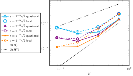
Figure 2: Relative errors $|||\mathbf{u}-u_{H}|||$ (quasilocal) and $|||\mathbf{u}-\tilde{u}_{H}|||$ (local) in dependence of the coarse mesh size $H$.

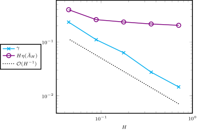
Figure 3: Model error estimators $H$ for $\varepsilon=2^{-7}\sqrt{2}$.

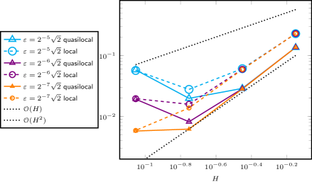
Figure 4: Relative errors $\|\mathbb{E}[\mathbf{u}_{h}]-u_{H}\|_{L^{2}(D)}$ (quasilocal) and $\|\mathbb{E}[\mathbf{u}_{h}]-\tilde{u}_{H}\|_{L^{2}(D)}$ (local) in dependence of the coarse mesh size $H$.

6 Conclusive comments

The proposed numerical homogenization procedure approximates the stochastic coefficient by the expectation of a quasilocal effective model. The design of intermediate stochastic models that carry more information on the stochastic dependence than a purely deterministic coefficient will be considered in future work. The presented error estimates are independent on any assumptions on the uncertainty and contain an a posteriori model error estimator $\gamma$. In the case that more structure on the coefficient is given, we expect that an a priori error estimate for $\gamma$ in terms of $H$ and $\varepsilon$ can be derived.

References

- [ACL+12] A. Anantharaman, R. Costaouec, C. Le Bris, F. Legoll, and F. Thomines. Introduction to numerical stochastic homogenization and the related computational challenges: some recent developments. In Multiscale modeling and analysis for materials simulation, volume 22 of Lect. Notes Ser. Inst. Math. Sci. Natl. Univ. Singap., pages 197–272. World Sci. Publ., Hackensack, NJ, 2012.
- [AKM17] S. Armstrong, T. Kuusi, and J.-C. Mourrat. The additive structure of elliptic homogenization. Invent. Math., 208(3):999–1154, 2017.
- [All92] G. Allaire. Homogenization and two-scale convergence. SIAM J. Math. Anal., 23(6):1482–1518, 1992.
- [AS16] S. N. Armstrong and C. K. Smart. Quantitative stochastic homogenization of convex integral functionals. Ann. Sci. Éc. Norm. Supér. (4), 49(2):423–481, 2016.
- [BJ11] G. Bal and W. Jing. Corrector theory for MSFEM and HMM in random media. Multiscale Model. Simul., 9(4):1549–1587, 2011.
- [BLP78] A. Bensoussan, J.-L. Lions, and G. Papanicolaou. Asymptotic Analysis for Periodic Structures. North-Holland Publ., 1978.
- [BP04] A. Bourgeat and A. Piatnitski. Approximations of effective coefficients in stochastic homogenization. Ann. Inst. H. Poincaré Probab. Statist., 40(2):153–165, 2004.
- [CS08] Z. Chen and T. Y. Savchuk. Analysis of the multiscale finite element method for nonlinear and random homogenization problems. SIAM J. Numer. Anal., 46(1):260–279, 2007/08.
- [DG75] E. De Giorgi. Sulla convergenza di alcune successioni d’integrali del tipo dell’area. Rend. Mat. (6), 8:277–294, 1975. Collection of articles dedicated to Mauro Picone on the occasion of his ninetieth birthday.
- [DGO16] M. Duerinckx, A. Gloria, and F. Otto. The structure of fluctuations in stochastic homogenization. arXiv e-prints, 1602.01717 [math.AP], 2016.
- [EMZ05] W. E, P. Ming, and P. Zhang. Analysis of the heterogeneous multiscale method for elliptic homogenization problems. J. Amer. Math. Soc., 18(1):121–156, 2005.
- [GH16] A. Gloria and Z. Habibi. Reduction in the resonance error in numerical homogenization II: Correctors and extrapolation. Found. Comput. Math., 16(1):217–296, 2016.
- [Glo12a] A. Gloria. Numerical approximation of effective coefficients in stochastic homogenization of discrete elliptic equations. ESAIM Math. Model. Numer. Anal., 46(1):1–38, 2012.
- [Glo12b] A. Gloria. Numerical homogenization: survey, new results, and perspectives. In Mathematical and numerical approaches for multiscale problem, volume 37 of ESAIM Proc., pages 50–116. EDP Sci., Les Ulis, 2012.
- [GMP10] V. Ginting, A. Målqvist, and M. Presho. A novel method for solving multiscale elliptic problems with randomly perturbed data. Multiscale Model. Simul., 8(3):977–996, 2010.
- [GNO14] A. Gloria, S. Neukamm, and F. Otto. A regularity theory for random elliptic operators. arXiv e-prints, 1409.2678, 2014.
- [GNO15] A. Gloria, S. Neukamm, and F. Otto. Quantification of ergodicity in stochastic homogenization: optimal bounds via spectral gap on Glauber dynamics. Invent. Math., 199(2):455–515, 2015.
- [GO11] A. Gloria and F. Otto. An optimal variance estimate in stochastic homogenization of discrete elliptic equations. Ann. Probab., 39(3):779–856, 2011.
- [GO12] A. Gloria and F. Otto. An optimal error estimate in stochastic homogenization of discrete elliptic equations. Ann. Appl. Probab., 22(1):1–28, 2012.
- [GO15] A. Gloria and F. Otto. The corrector in stochastic homogenization: optimal rates, stochastic integrability, and fluctuations. arXiv e-prints, 1510.08290 [math.AP], 2015.
- [GO17] A. Gloria and F. Otto. Quantitative results on the corrector equation in stochastic homogenization. J. Eur. Math. Soc. (JEMS), 19(11):3489–3548, 2017.
- [GP15] D. Gallistl and D. Peterseim. Stable multiscale Petrov-Galerkin finite element method for high frequency acoustic scattering. Comput. Methods Appl. Mech. Eng., 295:1–17, 2015.
- [GP17] D. Gallistl and D. Peterseim. Computation of quasilocal effective diffusion tensors and connections to the mathematical theory of homogenization. Multiscale Model. Simul., 15(4), 2017.
- [HP13] P. Henning and D. Peterseim. Oversampling for the multiscale finite element method. Multiscale Model. Simul., 11(4):1149–1175, 2013.
- [JKO94] V. V. Jikov, S. M. Kozlov, and O. A. Oleinik. Homogenization of Differential Operators and Integral Functionals. Springer-Verlag, 1994.
- [JMSDO14] J. Jagalur Mohan, O. Sahni, A. Doostan, and A. A. Oberai. Variational multiscale analysis: the fine-scale Green’s function for stochastic partial differential equations. SIAM/ASA J. Uncertain. Quantif., 2(1):397–422, 2014.
- [Koz79] S. M. Kozlov. The averaging of random operators. Mat. Sb. (N.S.), 109(151)(2):188–202, 327, 1979.
- [KPY18] R. Kornhuber, D. Peterseim, and H. Yserentant. An analysis of a class of variational multiscale methods based on subspace decomposition. Math. Comp., 87:2765–2774, 2018.
- [KY16] R. Kornhuber and H. Yserentant. Numerical homogenization of elliptic multiscale problems by subspace decomposition. Multiscale Modeling & Simulation, 14(3):1017–1036, 2016.
- [LLT14] C. Le Bris, F. Legoll, and F. Thomines. Multiscale finite element approach for “weakly” random problems and related issues. ESAIM Math. Model. Numer. Anal., 48(3):815–858, 2014.
- [MP14] A. Målqvist and D. Peterseim. Localization of elliptic multiscale problems. Math. Comp., 83(290):2583–2603, 2014.
- [MT78] F. Murat and L. Tartar. H-convergence. Séminaire d’Analyse Fonctionnelle et Numérique de l’Université d’Alger, 1978.
- [Ngu89] G. Nguetseng. A general convergence result for a functional related to the theory of homogenization. SIAM J. Math. Anal., 20(3):608–623, 1989.
- [Pet16] D. Peterseim. Variational multiscale stabilization and the exponential decay of fine-scale correctors. In G. R. Barrenechea, F. Brezzi, A. Cangiani, and E. H. Georgoulis, editors, Building Bridges: Connections and Challenges in Modern Approaches to Numerical Partial Differential Equations, volume 114 of Lect. Notes Comput. Sci. Eng., pages 341–367. Springer, 2016.
- [PV81] G. C. Papanicolaou and S. R. S. Varadhan. Boundary value problems with rapidly oscillating random coefficients. In Random fields, Vol. I, II (Esztergom, 1979), volume 27 of Colloq. Math. Soc. János Bolyai, pages 835–873. North-Holland, Amsterdam-New York, 1981.
- [Spa68] S. Spagnolo. Sulla convergenza di soluzioni di equazioni paraboliche ed ellittiche. Ann. Scuola Norm. Sup. Pisa (3) 22 (1968), 571-597; errata, ibid. (3), 22:673, 1968.
- [Yur86] V. V. Yurinskiĭ. Averaging of symmetric diffusion in a random medium. Sibirsk. Mat. Zh., 27(4):167–180, 215, 1986.
- [ZCH15] Z. Zhang, M. Ci, and T. Y. Hou. A multiscale data-driven stochastic method for elliptic PDEs with random coefficients. Multiscale Model. Simul., 13(1):173–204, 2015.
Acknowledgment
D. Gallistl acknowledges support by the Deutsche Forschungsgemeinschaft (DFG) through CRC 1173. Main parts of this paper were written while the authors enjoyed the kind hospitality of the Hausdorff Institute for Mathematics in Bonn during the trimester program on multiscale problems.