Thermal Inflation with a Thermal Waterfall Scalar Field Coupled to a Light Spectator Scalar Field

A new model of thermal inflation is introduced, in which the mass of the thermal waterfall field is dependent on a light spectator scalar field. Using the $\delta N$ formalism, the “end of inflation” scenario is investigated in order to ascertain whether this model is able to produce the dominant contribution to the primordial curvature perturbation. A multitude of constraints are considered so as to explore the parameter space, with particular emphasis on key observational signatures. For natural values of the parameters, the model is found to yield a sharp prediction for the scalar spectral index and its running, well within the current observational bounds.

1 Introduction

Cosmological Inflation is the leading candidate for the solution of the three main problems of the standard Big Bang cosmology: the horizon, flatness and relic problems. It also has the ability to seed the initial conditions required to explain the observed large-scale structure of the Universe [1]. In the simplest scenario, quantum fluctuations of a scalar field are converted to classical perturbations around the time of horizon exit, after which they become frozen. This gives rise to the primordial curvature perturbation, $\zeta$, which grows under the influence of gravity to give rise to the large-scale structure in the Universe. The simple single-field inflationary scenario is favoured by current observations [2]. However, given the richness and complexity of the theories beyond the standard model, this simple picture seems unlikely.

Moving away from this simplest scenario, there has been much work done on generating the observed $\zeta$ in other scenarios, such as the curvaton [3, 4, 5, 6, 7, 8, 9, 10, 11, 12, 13, 14], inhomogeneous reheating [15, 16, 17, 5, 18, 19, 20, 10, 11, 12, 13], “end of inflation” [21, 9, 20, 22, 23, 24, 25, 26] (also see [27]) and inhomogeneous phase transition [28] (also see [29]).

One particular model of inflation is thermal inflation [30, 31, 32, 33], which is a brief period of inflation that could have occurred after a period of prior primordial inflation. Thermal inflation lasts too little to solve the problems of the standard Big Bang cosmology that motivate primordial inflation, but it may be rather useful to dilute any dangerous relics that are not dealt with by primordial inflation such as moduli fields or gravitinos. Another interesting byproduct of thermal inflation is changing the number of e-folds before the end of primordial inflation, which correspond to the cosmological scales. This has an immediate effect on inflationary observables and can assist in inflation model building [34, 35].

Thermal inflation occurs due to finite-temperature effects arising from a coupling between a so-called thermal waterfall scalar field $\phi$ and the thermal bath created from the partial or complete reheating from primordial inflation. Thermal field theory gives a thermal contribution $g^{2}T^{2}\phi^{2}$ to the effective scalar potential, where $g$ is the coupling constant of the interaction between $\phi$ and the thermal bath and $T$ is the bath’s temperature. This results in a thermal correction to the effective mass of $g^{2}T^{2}$. This thermal mass can temporarily trap the thermal waterfall field on top of a false vacuum, resulting in inflation. However, as time goes by, the thermal mass of $\phi$ decreases such that a phase transition sends $\phi$ to its vacuum expectation value (VEV) and inflation is terminated.

Despite occurring much later than primordial inflation, thermal inflation may produce a substantial contribution to the curvature perturbation. This is how. The mass of a given scalar field may depend on the expectation value of another scalar field. [18, 19, 21, 28, 9, 16, 17, 22, 23, 24, 29, 13]. More specifically, the mass of a thermal waterfall field $\phi$ that is responsible for a bout of thermal inflation could be dependent on another scalar field $\psi$. We will call this $\psi$ a spectator field, because it needs not affect the dynamics of the Universe at any time. If $\psi$ is light during primordial inflation, its quantum fluctuations are converted to almost scale-invariant classical field perturbations at around the time of horizon exit. If $\psi$ remains light all the way up to the end of thermal inflation, then thermal inflation will end at different times in different parts of the Universe, because the value of the spectator field determines the mass of the thermal waterfall field $\phi$, which in turn determines the end of thermal inflation. This is the “end of inflation” mechanism [21] and it can generate a contribution to the primordial curvature perturbation $\zeta$. The motivation of this work is to explore this scenario to see if it can produce the dominant contribution to the primordial curvature perturbation with characteristic observational signatures, in which the inflaton’s contribution to the perturbation can be ignored. As such, inflation model building is liberated from the requirements to generate $\zeta$, which substantially reduces fine-tuning and renders viable many otherwise observationally excluded inflation models [37].

It should be noted that this scenario is very similar to that in Ref. [20]. However, in that paper the authors use a modulated coupling constant rather than a modulated mass. Also, the treatment that has been given to the work in this paper is much more comprehensive. One example of this is in the consideration of the effect that the thermal fluctuation of the thermal waterfall field has on the model (see Section 4.2.6). Another example is the requirement that the thermal waterfall field is thermalized (see Section 4.2.7). Also, there is no consideration given in Ref. [20] to requiring a fast transition from thermal inflation to thermal waterfall field oscillation (see LABEL:Subsubsection:_Time_of_Transition_from_Thermal_Inflation_to_ThermalWaterfall_Field_Oscillation), as detailed in Ref. [24], as this paper appeared after Ref. [20].

This paper is structured as follows. In Section 2 we introduce our new model. In Section 3 we give expressions for key observational quantities that are predicted by the model. In Section 4 we explore the “end of inflation” scenario and obtain in detail a multitude of constraints for our model parameters. We conclude in Section 5.

Throughout this work, natural units are used where $c\!=\!\hbar\!=\!k_{B}\!=\!1$ and Newton’s gravitational constant is $8\pi G=M_{P}^{-2}$, with $M_{P}\!=\!2.436\times 10^{18}\ \mbox{GeV}$ being the reduced Planck Mass.

2 A new Thermal Inflation model

The potential that we consider in our model is

$$V(\phi,\psi,T)= V_{0}+\left(g^{2}T^{2}-\frac{1}{2}m_{0}^{2}+h^{2}\frac{\psi^{2\alpha}}{M_{P}^{2\alpha-2}}\right)\phi^{2}$$

$$+\lambda\frac{\phi^{2n+4}}{M_{P}^{2n}}+\frac{1}{2}m_{\psi}^{2}\psi^{2},$$ (2.1)

where $\phi$ is the thermal waterfall scalar field, $\psi$ is a light spectator scalar field, $T$ is the temperature of the thermal bath, $g$, $h$ and $\lambda$ are dimensionless coupling constants, $\alpha\geq 1$ and $n\geq 1$ are integers, $V_{0}$ is a density scale (corresponding to the scale of thermal inflation) and the $-m_{0}^{2}$ and $m_{\psi}^{2}$ are soft mass-squared terms coming form supersymmetry (SUSY) breaking. A $\phi^{4}$ term is not featured because the thermal waterfall field is a flaton, whose potential is stabilised by the higher-order non-renormalisable term [30, 31]. The non-renormalisable terms in Eq. 2.1 are the dominant terms in series over $\alpha$ and $n$. One would expect the lowest order to be dominant. Indeed, we find that parameter space exists only if $\alpha=n=1$. Thus, we chose these values in this paper. With this choice, the potential in Eq. 2.1 becomes

$$V(\phi,\psi,T)= V_{0}+\left(g^{2}T^{2}-\frac{1}{2}m_{0}^{2}+h^{2}\psi^{2}\right)\phi^{2}$$

$$+\lambda\frac{\phi^{6}}{M_{P}^{2}}+\frac{1}{2}m_{\psi}^{2}\psi^{2},$$ (2.2)

We make the following definition

$$m^{2}\equiv m_{0}^{2}-2h^{2}\psi^{2}\,.$$ (2.3)

The variation of $m(\psi)$ is

$$\delta m=-\frac{2h^{2}\psi}{m}\,\delta\psi\,.$$ (2.4)

We only consider the case where the mass of $\phi$ is coupled to one field. Were the mass coupled to several similar fields, the results would be just multiplied by the number of fields. If the multiple fields are different, then there will be only a small number that dominate the contribution to the mass perturbation. Therefore we consider only one for simplicity.

Using Eq. 2.3, the potential becomes

$$V(\phi,\psi,T)= V_{0}+\left(g^{2}T^{2}-\frac{1}{2}m^{2}\right)\phi^{2}$$

$$+\lambda\frac{\phi^{6}}{M_{P}^{2}}+\frac{1}{2}m_{\psi}^{2}\psi^{2}\,.$$ (2.5)

This potential is shown in Fig. 1.

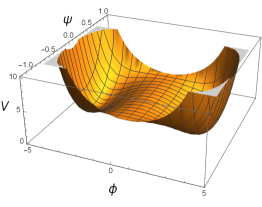
Arbitrary Units

Fig. 1: The potential given by Eq. 2.5.

It would appear from the potential that domain walls will be produced, due to the fact that in some parts of the Universe $\phi$ will roll down to $+\left\langle\phi\right\rangle$ while in others parts it will roll down to $-\left\langle\phi\right\rangle$. However, being a flaton field (i.e. a flat direction in SUSY) $\phi$ is a complex field, whose potential contains only one continuous vacuum expectation value (VEV).

The zero temperature potential is

$$V(\phi,\psi,0)=V_{0}-\frac{1}{2}m^{2}\phi^{2}+\lambda\frac{\phi^{6}}{M_{P}^{2}}+\frac{1}{2}m_{\psi}^{2}\psi^{2}\,.$$ (2.6)

Hence, the VEV is

$$\left\langle\phi\right\rangle\sim\left(\frac{mM_{P}}{\sqrt{\lambda}}\right)^{1/2}.$$ (2.7)

$V_{0}$ is obtained by requiring $V(\langle\phi\rangle)=0$ along the $\psi\!=\!0$ direction. We find

$$V_{0}\sim\frac{m_{0}^{3}M_{P}}{\sqrt{\lambda}}\,.$$ (2.8)

Now, we use the Friedmann equation

$$M_{P}^{2}H_{\textrm{TI}}^{2}\sim V_{0}\;,$$ (2.9)

to obtain the Hubble parameter during thermal inflation as

$$H_{\textrm{TI}}\sim\left(\frac{m_{0}^{3}}{\sqrt{\lambda}\,M_{P}}\right)^{1/2}.$$ (2.10)

Within this thermal inflation model there are two cases regarding the decay rate of the inflaton field $\Gamma_{\varphi}$, with $\varphi$ being the inflaton, i.e. the field driving primordial inflation prior to thermal inflation. One is the case when $\Gamma_{\varphi}\!\gtrsim\!H_{\textrm{TI}}$, i.e. that reheating from primordial inflation occurs before or around the time of the start of thermal inflation. Alternatively, there is the case when $\Gamma_{\varphi}\!\ll\!H_{\textrm{TI}}$, i.e. that reheating from primordial inflation occurs at some time after the end of thermal inflation.

In the case of $\Gamma_{\varphi}\!\gtrsim\!H_{\textrm{TI}}$, thermal inflation begins at a temperature

$$T_{1}\sim V_{0}^{1/4}$$ (2.11)

$T_{1}$ corresponds to the temperature when the potential energy density becomes comparable with the energy density of the thermal bath, for which the density is $\rho_{\gamma}\!\sim\!T^{4}$.

In the case of $\Gamma_{\varphi}\!\ll\!H_{\textrm{TI}}$, thermal inflation begins at a temperature

$$T_{1}\sim\left(M_{P}^{2}\,H_{\textrm{TI}}\Gamma_{\varphi}\right)^{1/4}$$ (2.12)

Initially, for $T\geq T_{1}$, the thermal waterfall field is driven to zero $\phi\rightarrow 0$ as the thermally induced mass in Eq. 2.5 is dominant. This continues even if $T<T_{1}$ as long as the mass squared of $\phi$ remains positive. When the tachyonic mass term of the thermal waterfall field becomes equal to the thermally-induced mass term (cf. Eq. 2.5) a phase transition sends the field towards its non-zero true VEV and thermal inflation ends [30].

In both of the above cases, thermal inflation ends at a temperature

$$T_{2}=\frac{m}{\sqrt{2}\,g}\,.$$ (2.13)

In the following, we only consider the case where $\Gamma_{\varphi}\!\ll\!H_{\textrm{TI}}$, in that reheating from primordial inflation occurs at some time after the end of thermal inflation, as this scenario was found to yield more parameter space than the case where $\Gamma_{\varphi}\!\gtrsim\!H_{\textrm{TI}}$.

3 $\phi$ Decay Rate, Spectral Index and Tensor Fraction

3.1 $\phi$ Decay Rate

The decay rate of $\phi$ is given by

$$\Gamma\sim\mathrm{max}\left\{g^{2}m\hskip 5.0pt,\hskip 5.0pt\frac{m^{3}}{M_{P}^{2}}\right\}$$ (3.1)

The first expression is for decay into the thermal bath via direct interactions and the second is for gravitational decay. We will only consider the case in which the direct decay is the dominant channel ($g$ is not taken to be very small). This is the case when $m\ll gM_{P}$. Therefore we have just $\Gamma\sim g^{2}m$.

3.2 Spectral Index and its running

Thermal Inflation has the effect of changing the number of e-folds before the end of primordial inflation at which cosmological scales exit the horizon. This affects the value of the spectral index $n_{s}$ of the curvature perturbation $\zeta$ (see for example [34, 35]).

We assume $\zeta$ is generated due to the perturbations of the spectator scalar field. Then, in the case of slow-roll inflation, the spectral index is given by [1]

$$n_{s}\simeq 1-2\epsilon+2\eta_{\psi}\;.$$ (3.2)

where $\epsilon$ and $\eta_{\psi}$ are slow-roll parameters, defined as

$$\epsilon\equiv\frac{M_{P}^{2}}{2}\left(\frac{V^{\prime}(\varphi)}{V(\varphi)}\right)^{2}\quad{\rm and}\quad\eta_{\psi}\equiv\frac{1}{3H^{2}}\frac{\partial^{2}V}{\partial\psi^{2}}\,,$$ (3.3)

where $V^{\prime}(\varphi)$ is the derivative of the inflaton potential with respect to the inflaton field $\varphi$. $\epsilon$ and $\eta_{\psi}$ are to be evaluated at the point where cosmological scales exit the horizon during primordial inflation.

Regarding the various scalar fields involved in this model, the reason why $\epsilon$ depends only on $\varphi$ is because this slow-roll parameter captures the inflationary dynamics of primordial inflation, which is governed only by $\varphi$ in our model (we are assuming that both $\psi$ and $\phi$ have settled to a constant value (LABEL:Subsubsection:The_Field_Value_phi_{*} and LABEL:Subsubsection:_The_Field_Value_psi_{*} respectively) by the time cosmological scales exit the horizon during primordial inflation). In a similar fashion, the reason why the slow-roll parameter $\eta_{\psi}$ depends only on $\psi$ is because this parameter captures the dependence on the spectral index of the field(s) whose perturbations contribute to the observed primordial curvature perturbation $\zeta$. In our case, this is only the spectator field $\psi$.

The definition of the running of the spectral index is [1]

$$n_{s}^{\prime}\equiv\frac{\mathrm{d}n_{s}}{\mathrm{d}\ln k}\simeq-\frac{\mathrm{d}n_{s}}{\mathrm{d}N}\,,$$ (3.4)

the second equation coming from $\mathrm{d}\ln k\!=\!\mathrm{d}\ln{(aH)}\!\simeq\!H\mathrm{d}t\!\equiv\!-\mathrm{d}N$, where $k\!=\!aH$. From Eq. 3.2, we have

$$n_{s}^{\prime}\simeq 2\frac{\mathrm{d}\epsilon}{\mathrm{d}N}-2\frac{\mathrm{d}\eta_{\psi}}{\mathrm{d}N}\simeq 2\epsilon\frac{\mathrm{d}\ln\epsilon}{\mathrm{d}N}-2\frac{\mathrm{d}\eta_{\psi}}{\mathrm{d}N}\,.$$ (3.5)

Now, we have [1]

$$\frac{\mathrm{d}\ln\epsilon}{\mathrm{d}N}\simeq-4\epsilon+2\eta\,,$$ (3.6)

where $\eta$ is a slow-roll parameter given by

$$\eta\equiv M_{P}^{2}\frac{V^{\prime\prime}(\varphi)}{V(\varphi)}\,.$$ (3.7)

Also,

$$\frac{\mathrm{d}\eta_{\psi}}{\mathrm{d}N}=-\frac{1}{3H^{4}}\frac{\mathrm{d}(H^{2})}{\mathrm{d}N}\frac{\partial^{2}V}{\partial\psi^{2}}=-2\eta_{\psi}\frac{\mathrm{d}\ln H}{\mathrm{d}N}\,,$$ (3.8)

where we used that $V(\psi)$ does not depend on $N$, as we are assuming that both $\psi$ and $\phi$ have settled to a constant value (LABEL:Subsubsection:The_Field_Value_phi_{*} and LABEL:Subsubsection:_The_Field_Value_psi_{*} respectively) by the time cosmological scales exit the horizon during primordial inflation.

Since [1],

$$\frac{\mathrm{d}\ln H}{\mathrm{d}N}\simeq\epsilon\,,$$ (3.9)

we have

$$\frac{\mathrm{d}\eta_{\psi}}{\mathrm{d}N}\simeq-2\epsilon\eta_{\psi}\;.$$ (3.10)

Therefore, the final result for the running of the spectral index is

$$n_{s}^{\prime}\simeq-8\epsilon^{2}+4\epsilon\eta+4\epsilon\eta_{\psi}\;.$$ (3.11)

From now on we assume that $H$ has the constant value $H_{\ast}$ by the time cosmological scales exit the horizon up until the end of primordial inflation. In order to obtain $\epsilon$ and $\eta$, we require the value of $N_{\ast}$, the number of e-folds before the end of primordial inflation at which cosmological scales exit the horizon. We consider the period between when the pivot scale, $k_{0}\!\equiv\!0.002\ \mbox{Mpc${}^{-1}$}$, exits the horizon during primordial inflation and when it reenters the horizon long after the end of thermal inflation. We have

$$R_{\ast}=H_{\ast}^{-1}\quad{\rm and}\quad(k_{0}/a_{\rm piv})^{-1}=H_{\textrm{piv}}^{-1}\;,$$ (3.12)

where $R_{\ast}$ is a length scale when the pivot scale exits the horizon during primordial inflation and the subscript ‘piv’ denotes the time when this scale re-enters the horizon, with $a$ being the scale factor of the Universe. Therefore

$$H_{\ast}^{-1}=\frac{a_{\ast}}{a_{\textrm{piv}}}H_{\textrm{piv}}^{-1}.$$ (3.13)

Using the above, we now can calculate $N_{*}$.

Since $\Gamma_{\varphi}\!\ll\!H_{\textrm{TI}}$, we have

$$e^{N_{\ast}}\!\!=\!\!\frac{H_{\ast}}{k}\!\left(\frac{T_{\textrm{start,TI}}}{T_{\textrm{end,inf}}}\right)^{\!\!8/3}\!\!\left(\frac{T_{\textrm{reh,TI}}}{T_{\textrm{end,TI}}}\right)^{\!\!8/3}\!\!\frac{T_{\textrm{piv}}e^{-N_{\textrm{TI}}}}{T_{\textrm{reh,TI}}}$$ (3.14)

where $N_{\textrm{TI}}$ is the number of e-folds of thermal inflation and the subscripts denote the following: ‘end,inf’ is at the end of primordial inflation, ‘start,TI’ is at the start of thermal inflation, ‘end,TI’ is at the end of thermal inflation and ‘reh,TI’ is at thermal inflation reheating. For the period between the end of primordial/thermal inflation and primordial/thermal inflation reheating, $a\propto{T}^{-8/3}$. For all other times, $a\propto T^{-1}$.

We need to calculate $T_{\textrm{piv}}$. We consider the period between when the pivot scale reenters the horizon and the present. Throughout this period the Universe is matter-dominated (ignoring dark energy). Therefore we have $\rho\propto a^{-3}\propto T^{3}$. Using the Friedmann equation, $3M_{P}^{2}H^{2}\propto T^{3}$ we have

$$\frac{H_{\textrm{piv}}^{2}}{H_{0}^{2}}=\frac{T_{\textrm{piv}}^{3}}{T_{0}^{3}}\;\Rightarrow\;T_{\textrm{piv}}=9.830\times 10^{-13}\ \mbox{GeV}$$ (3.15)

where ‘0’ denotes the values at present. Using this, we obtain $N_{\ast}$ as

$$N_{\ast}\approx\ln{\left(\frac{\left(3.2\times 10^{37}\ \mbox{GeV${}^{-1}$}\right)H_{\ast}}{0.002}\right)}+\frac{2}{3}\ln{\left(\frac{\Gamma}{H_{\ast}}\right)}\\ +\frac{1}{4}\ln{\left(\frac{10\pi^{2}\left(9.8\times 10^{-13}\ \mbox{GeV}\right)^{4}}{9M_{P}^{2}\Gamma^{2}}\right)}-N_{\textrm{TI}}\,,$$ (3.16)

where we have used $g_{\ast}\!\approx\!10^{2}$ as the number of spin states (effective relativistic degrees of freedom) of the particles in the thermal bath, at the time of both primordial inflation reheating and thermal inflation reheating.

3.3 Tensor Fraction $r$

The definition of the tensor fraction is $r\equiv\mathcal{P}_{h}/\mathcal{P}_{\zeta}\;$ [1], where $\mathcal{P}_{h}$ and $\mathcal{P}_{\zeta}$ are the spectra of the primordial tensor and curvature perturbations respectively. The spectrum $\mathcal{P}_{h}$ is given by

$$\mathcal{P}_{h}(k)=\frac{8}{M_{P}^{2}}\left(\frac{H_{k}}{2\pi}\right)^{2}$$ (3.17)

for a given wavenumber $k$. Using this, together with $\rho_{\ast}\!=\!3M_{P}^{2}H_{\ast}^{2}$, given that we are saying $H_{k}\!=\!H_{\ast}$ for our current case, as well as the observed value $\mathcal{P}_{\zeta}(k_{0})\!=\!2.142\times 10^{-9}$, we obtain

$$r=\left(\frac{\rho_{\ast}^{1/4}}{3.25\times 10^{16}\ \mbox{GeV}}\right)^{4}$$ (3.18)

4 End-of-Inflation Mechanism

In this section we investigate the “end of inflation” mechanism. We aim to obtain a number of constraints on the model parameters and the initial conditions for the fields. Considering these constraints, we intend to determine the available parameter space. In this parameter space we will calculate distinct observational signatures that may test this scenario in the near future.

4.1 Generating $\zeta$

As $\phi$ is coupled to $\psi$, the “end of inflation” mechanism will generate a contribution to the primordial curvature perturbation $\zeta$ [21]. We use the $\delta N$ formalism to calculate this contribution as

$$\zeta\!=\!\delta N_{\textrm{TI}}=\!\frac{\mathrm{d}N_{\textrm{TI}}}{\mathrm{d}m}\delta m+\frac{1}{2!}\frac{\mathrm{d^{2}}N_{\textrm{TI}}}{\mathrm{d}m^{2}}\delta m^{2}+\frac{1}{3!}\frac{\mathrm{d^{3}}N_{\textrm{TI}}}{\mathrm{d}m^{3}}\delta m^{3}+\cdots\,.$$ (4.1)

The number of e-folds between the start and end of thermal inflation is given by

$$N_{\textrm{TI}}=\ln{\left(\frac{a_{2}}{a_{1}}\right)}=\ln{\left(\frac{T_{1}}{T_{2}}\right)}\,,$$ (4.2)

where $a_{1}\!=\!a_{\textrm{start,TI}}$ and $a_{2}\!=\!a_{\textrm{end,TI}}$.

Substituting $T_{1}$ and $T_{2}$, LABEL:Eq.:_T_{1}_(Gamma_{varphi}_<<_H_{TI}) and LABEL:Eq.:_T_{2} respectively, into Eq. 4.2 gives

$$N_{\textrm{TI}} \simeq\ln{\left[\frac{\sqrt{2}\,g\left(M_{P}^{2}\,H_{\textrm{TI}}\Gamma_{\varphi}\right)^{1/4}}{m}\right]}$$

$$\simeq\frac{1}{8}\ln\left(\frac{g^{8}}{\sqrt{\lambda}}\frac{M_{P}^{3}\Gamma_{\varphi}^{2}}{m^{5}}\right),$$ (4.3)

where we used LABEL:Eq.:_H_{TI}

Therefore the $\delta N$ formalism to third order gives

$$\zeta=\delta N_{\textrm{TI}}=-\frac{5}{8}\frac{\delta m}{m}+\frac{5}{16}\frac{\delta m^{2}}{m^{2}}-\frac{5}{24}\frac{\delta m^{3}}{m^{3}}\,.$$ (4.4)

By substituting our mass definition and its differential, Eqs. 2.3 and 2.4, into LABEL:Eq.:_Zeta_(m)_(Gamma_{varphi}_<<_H_{TI}) we obtain the power spectrum of the primordial curvature perturbation, which to first order is

$$\sqrt{\mathcal{P}_{\zeta}}=\frac{5}{8\pi}\frac{h^{2}H_{\ast}\psi}{m^{2}}\,.$$ (4.5)

A required condition for the perturbative expansion in LABEL:Eq.:_Zeta_(m)_(Gamma_{varphi}_<<_H_{TI}) to be suitable is that each term is much smaller than the preceding one. This requirement gives

$$\frac{h^{2}H_{\ast}\psi}{m^{2}}\ll 1\,,$$ (4.6)

which is readily satisfied as $\sqrt{\mathcal{P}_{\zeta}}\ll 1$.

4.2 Constraining the Parameters

In this section we produce a number of constraints for the model parameters and we describe the rationale behind them.

4.2.1 Primordial Inflation Energy Scale

We want the energy scale of primordial inflation to be $V^{1/4}\lesssim 10^{14}\,$GeV so that the inflaton contribution to the curvature perturbation is negligible. Therefore, from the Friedmann equation we require

$$H_{\ast}\lesssim 10^{10}\ \mbox{GeV}$$ (4.7)

4.2.2 Thermal Inflation Dynamics

We will consider only the case in which the inflationary trajectory is 1-dimensional, in that only the $\phi$ field is involved in determining the trajectory of thermal inflation in field space. We do this only to work with the simplest scenario for the trajectory. It is not a requirement on the model itself. In order that the $\psi$ field does not affect the inflationary trajectory during thermal inflation, we require from our $m$ mass definition, Eq. 2.3, that

$$m_{0}\gtrsim h\psi\,.$$ (4.8)

Therefore we have $m\simeq m_{0}\;$.

From our potential, at the onset of thermal inflation, Eq. 2.2, LABEL:Eq.:_m_{0}_>>_Coupling_Term gives

$$m_{0}^{2}<2g^{2}T_{1}^{2}.$$ (4.9)

For $\Gamma_{\varphi}\!\ll\!H_{\textrm{TI}}$, substituting $T_{1}$ from LABEL:Eq.:_T_{1}_(Gamma_{varphi}_<<_H_{TI}) into LABEL:Eq.:_m_{0}^{2}<2g^{2}T_{1}^{2} gives

$$m_{0}<\left[\left(g^{4}\Gamma_{\varphi}\right)^{2}\frac{M_{P}^{3}}{\sqrt{\lambda}}\right]^{1/5}.$$ (4.10)

4.2.3 Lack of Observation of $\phi$ Particles

Given that we have not observed any $\phi$ particles, the constraint on the present value of the effective mass of $\phi$ is $m_{\phi,\textrm{now}}\gtrsim 1\,$TeV. From our potential, Eq. 2.2, we have $m_{\phi,\textrm{now}}^{2}\sim-m_{0}^{2}+30\lambda\left\langle\phi\right\rangle^{4}/M_{P}^{2}$. Substituting the VEV of $\phi$, Eq. 2.7, into here gives $m_{\phi,\textrm{now}}\sim m_{0}$ for all reasonable values of $n$. Therefore, we require

$$m_{0}\gtrsim 1\ \mbox{TeV}\,.$$ (4.11)

4.2.4 Light auxiliary field $\psi$

In order that $\psi$ acquires classical perturbations during primordial inflation, we require $\psi$ to be light during this time, i.e. $|m_{\psi,\textrm{eff}}|\ll H_{\ast}$, where we are using notation such that $|m_{\psi,\textrm{eff}}|\equiv\sqrt{\left|m_{\psi,\textrm{eff}}^{2}\right|}$. We have

$$m_{\psi,\textrm{eff}}^{2}=m_{\psi}^{2}+2h^{2}\phi^{2}\,.$$ (4.12)

Therefore we need

$$m_{\psi}<H_{\ast}\quad{\rm and}\quad h\phi_{\ast}<H_{\ast}\;,$$ (4.13)

where $\phi_{\ast}$ and $\psi_{\ast}$ are the values of $\phi$ and $\psi$ during primordial inflation respectively.

We require that $\psi$ remains at $\psi_{\ast}$, the value during primordial inflation, all the way up to the end of thermal inflation. The reason for this is that if $\psi$ started to move, then its perturbation would decrease. This is because $\psi$ unfreezes when the Hubble parameter becomes less than $\psi$’s mass, i.e. $H\!<\!m_{\psi}$. In this case, the perturbation of $\psi$ also unfreezes, because it has the same mass as $\psi$. The density of the oscillating $\psi$ field decreases as matter, so $m_{\psi}^{2}\psi^{2}\!\propto\!a^{-3}\Rightarrow\psi\!\propto\!a^{-3/2}$. The same is true for the perturbation, i.e. $\delta\psi\!\propto\!a^{-3/2}$. So the whole effect of perturbing the end of thermal inflation is diminished. Requiring that $\psi$ is light at all times up until the end of thermal inflation is sufficient to ensure that the field and its perturbation remain at $\psi_{\ast}$ and $\delta\psi_{\ast}$ respectively. Therefore we require

$$m_{\psi}<H_{\textrm{TI}}$$ (4.14)

which is of course stronger than just $m_{\psi}\!\ll\!H_{\ast}$ in LABEL:Eq.:_2nd_Term_Psi_Effective_Mass_<<_H_{*}.

Similarly to $\phi$, given that we have not observed any $\psi$ particles, the most liberal constraint on the present value of the effective mass of $\psi$ is

$$m_{\psi,\textrm{now}}\gtrsim 1\ \mbox{TeV}$$ (4.15)

4.2.5 The Field Value $\psi_{\ast}$

Substituting the observed spectrum value $\mathcal{P}_{\zeta}(k_{0})\!=\!2.142\times 10^{-9}$ into LABEL:Eq.:_Power_Spectrum_(Gamma_{varphi}_<<_H_{TI}) gives the constraint

$$\psi_{\ast}\sim 10^{-4}\,\frac{m_{0}^{2}}{h^{2}H_{\ast}}\,.$$ (4.16)

Substituting LABEL:Eq.:_Psi_{*} into LABEL:Eq.:_m_{0}_>>_Coupling_Term, regarding the dynamics of thermal inflation, gives

$$h\gtrsim 10^{-4}\,\frac{m_{0}}{H_{\ast}}\,.$$ (4.17)

Rearranging this for $m_{0}$ gives the constraint

$$m_{0}\lesssim 10^{4}\,hH_{\ast}\;.$$ (4.18)

We require the field value of $\psi$ to be much larger than its perturbation, i.e. $\psi_{\ast}\gg\delta\psi_{\ast}$, so that the perturbative approach is valid. Therefore, with $\delta\psi_{\ast}\sim H_{\ast}$, we obtain

$$\psi_{\ast}\gg H_{\ast}\quad{\rm and}\quad\frac{\delta\psi_{\ast}}{\psi_{\ast}}\ll 1\,.$$ (4.19)

Combining the frozen value $\psi_{\ast}$, LABEL:Eq.:_Psi_{*}, with the above gives

$$m_{0}>10^{2}\,hH_{\ast}\;.$$ (4.20)

Thus, we find the following range

$$10^{2}<\frac{m_{0}}{hH_{*}}<10^{4}.$$ (4.21)

4.2.6 Thermal Fluctuation of $\phi$

The effective mass of $\phi$ at the end of primordial inflation is

$$m_{\phi,\textrm{end,inf}}^{2}\sim g^{2}T_{\textrm{end,inf}}^{2}-m_{0}^{2}\sim g^{2}\,T_{\textrm{end,inf}}^{2}\;,$$ (4.22)

since $gT_{\textrm{end,inf}}\!\gg\!m_{0}$ [36].

As we are dealing with the thermal fluctuation of $\phi$ about $\phi\!=\!0$, we have $\left\langle\delta\phi\right\rangle_{T}\!=\!\left\langle\phi\right\rangle_{T}$. The thermal fluctuation of $\phi$ is

$$\sqrt{\left\langle\phi^{2}\right\rangle_{T}}\sim T$$ (4.23)

and we require [36]

$$g<1\,,$$ (4.24)

because $g$ is a perturbative coupling.

In order to keep $m_{\psi,\textrm{eff}}$ light, we require (cf.Section 4.2.4),

$$hT_{1}<H_{\textrm{TI}}\;.$$ (4.25)

During the time between the end of primordial inflation and primordial inflation reheating, $T\!\propto\!a^{-3/8}$ and $H\!\propto\!a^{-3/2}$. Therefore, if Eq. 4.25 is satisfied, then equivalent constraints for higher $T$ and $H$ are guaranteed to be satisfied as well.

Considering $\Gamma_{\varphi}\!\ll\!H_{\textrm{TI}}$, by substituting LABEL:Eq.:_H_{TI}, LABEL:Eq.:_Psi_{*} and LABEL:Eq.:_T_{1}_(Gamma_{varphi}_<<_H_{TI}) into Eq. 4.25 we obtain the constraint

$$h<\left(\lambda^{-3/2}\frac{m_{0}^{9}}{M_{P}^{7}\Gamma_{\varphi}^{2}}\right)^{1/8}$$ (4.26)

Rearranging this for $m_{0}$ gives

$$m_{0}>\left(\lambda^{3/2}h^{8}M_{P}^{7}\Gamma_{\varphi}^{2}\right)^{1/9}.$$ (4.27)

4.2.7 Thermalization of $\phi$

In order that $\phi$ interacts with the thermal bath and therefore that we actually have the $g^{2}T^{2}\phi^{2}$ term in our potential, Eq. 2.2, we require $\Gamma_{\textrm{therm}}>H$, where $\Gamma_{\textrm{therm}}$ is the thermalization rate of $\phi$, which is given by

$$\Gamma_{\textrm{therm}}=n\left\langle\sigma v\right\rangle\sim\sigma\,T^{3}\,,$$ (4.28)

where $n\!\sim\!T^{3}$ is the number density of particles in the thermal bath, $\sigma$ is the scattering cross-section for the interaction of $\phi$ and the particles in the thermal bath, $v$ is the relative velocity between a $\phi$ particle and a thermal bath particle (which in our case is $\approx\!c\!=\!1$) and $\left\langle\,\right\rangle$ denotes a thermal average. The scattering cross-section $\sigma$ is given by

$$\sigma\sim\frac{g^{4}}{E_{\textrm{cm}}^{2}}\,,$$ (4.29)

where $E_{\textrm{cm}}$ is the centre-of-mass energy, which is $E_{\textrm{cm}}\sim T$. Substituting this into Eq. 4.29 gives

$$\sigma\sim\frac{g^{4}}{T^{2}}\,.$$ (4.30)

This scattering cross-section is the total cross-section for all types of scattering (e.g. elastic) that can take place between $\phi$ and the particles in the thermal bath. The thermalization rate now becomes

$$\Gamma_{\textrm{therm}}\sim g^{4}T\,.$$ (4.31)

As before, during the time between the end of primordial inflation and primordial inflation reheating, $T\!\propto\!a^{-3/8}$ and $H\!\propto\!a^{-3/2}$. Therefore, if the constraint $\Gamma_{\textrm{therm}}\!>\!H$ is satisfied at the time of the end of primordial inflation, then it is satisfied all the way up to the start of thermal inflation. Thus, we have the constraint

$$\Gamma_{\textrm{therm}}\gtrsim H_{\ast}\,.$$ (4.32)

Taking Eq. 4.31 with $T\!\sim\!\left(M_{P}^{2}\,H_{\ast}\,\Gamma_{\varphi}\right)^{1/4}$ gives

$$\Gamma_{\varphi}\gtrsim\frac{H_{\ast}^{3}}{g^{16}M_{P}^{2}}\,.$$ (4.33)

We also require $\Gamma_{\textrm{therm}}\!>\!H$ to be satisfied throughout the whole of thermal inflation. Therefore, we have the constraint

$$g^{4}\,T_{2}>H_{\textrm{TI}}\;.$$ (4.34)

Substituting $H_{\textrm{TI}}$ and $T_{2}$, LABEL:Eq.:_T_{2} and LABEL:Eq.:_H_{TI} into the above gives

$$m_{0}<g^{6}\sqrt{\lambda}\,M_{P}\;.$$ (4.35)

4.2.8 The Field Value $\phi_{\ast}$

We consider two possible cases for the value of the thermal waterfall field $\phi$ during primordial inflation, with $m_{\phi,\textrm{inf}}$ being the effective mass of $\phi$ during primordial inflation:

1. $\phi$ heavy, i.e. $|m_{\phi,\textrm{inf}}|\gg H_{\ast}$, in which $\phi$ rolls down to its VEV.

2. $\phi$ light, i.e. $|m_{\phi,\textrm{inf}}|\ll H_{\ast}$, in which $\phi$ is at the Bunch-Davies value (to be explained below).

Case A
Substituting $\left\langle\phi\right\rangle$, Eq. 2.7, into LABEL:Eq.:_2nd_Term_Psi_Effective_Mass_<<_H_{*} gives

$$h<\lambda^{1/4}\frac{H_{\ast}}{\sqrt{m_{0}M_{P}}}\,.$$ (4.36)

Rearranging this for $m_{0}$ gives

$$m_{0}<\frac{\sqrt{\lambda}}{h^{2}}\,\frac{H_{\ast}^{2}}{M_{P}}\,.$$ (4.37)

Case B
We consider $\phi$ to be at the Bunch-Davies value

$$\phi_{\textrm{BD}}\sim\left(\frac{M_{P}H_{\ast}^{2}}{\sqrt{\lambda}}\right)^{1/3},$$ (4.38)

corresponding to the Bunch-Davies vacuum [39], which is the unique quantum state that corresponds to the vacuum, i.e. no particle quanta, in the infinite past in conformal time in a de Sitter spacetime. $\phi_{\textrm{BD}}$ is of this form as $\lambda\phi^{6}/M_{P}^{2}\sim H_{\ast}^{4}$, this being because the probability of this Bunch-Davies state is proportional to the factor $e^{-V/H^{4}}$ [40].

Substituting $\phi_{\textrm{BD}}$, Eq. 4.38, into LABEL:Eq.:_2nd_Term_Psi_Effective_Mass_<<_H_{*} gives

$$h<\lambda^{1/6}\left(\frac{H_{\ast}}{M_{P}}\right)^{1/3}.$$ (4.39)

4.2.9 Energy Density of $\phi$

We require the energy density of $\phi$ to be subdominant at all times, in order that it does not cause any inflation by itself. During the period between the end of primordial inflation and the start of thermal inflation, the energy density of $\phi$ is

$$\rho_{\phi}\sim g^{2}T^{2}\phi^{2}\sim g^{2}T^{4},$$ (4.40)

the second equation coming from the thermal fluctuation $\phi\sim\!T$. Therefore, considering the Friedmann equation, we require

$$g\,T_{1}^{2}<M_{P}H_{\textrm{TI}}\;.$$ (4.41)

During the time between the end of primordial inflation and primordial inflation reheating, $T\!\propto\!a^{-3/8}$ and $H\!\propto\!a^{-3/2}$. Therefore, if LABEL:Eq.:_gT_{1}^{2}_<<_M_{P}H_{TI} is satisfied, then equivalent constraints for higher $T$ and $H$ are guaranteed to be satisfied as well.

Using that $\Gamma_{\varphi}\!\ll\!H_{\textrm{TI}}$, by substituting $H_{\textrm{TI}}$ and $T_{1}$, LABEL:Eq.:_T_{1}_(Gamma_{varphi}_<<_H_{TI}) and LABEL:Eq.:_H_{TI} into LABEL:Eq.:_gT_{1}^{2}_<<_M_{P}H_{TI} we obtain

$$m_{0}>\left[\left(g^{2}\Gamma_{\varphi}\right)^{2}\sqrt{\lambda}\,M_{P}\right]^{1/3}.$$ (4.42)

$\phi_{\ast}$ Case A
The energy density of $\phi$ during primordial inflation is

$$\rho_{\phi,\textrm{inf}} =\left(-\frac{1}{2}m_{0}^{2}+h^{2}\psi_{\ast}^{2}\right)\left\langle\phi\right\rangle^{2}+\lambda\frac{\left\langle\phi\right\rangle^{6}}{M_{P}^{2}}$$

$$\sim-\frac{1}{2}m_{0}^{2}\left\langle\phi\right\rangle^{2}+\lambda\frac{\left\langle\phi\right\rangle^{6}}{M_{P}^{2}}\,,$$ (4.43)

with the second equation coming from LABEL:Eq.:_m_{0}_>>_Coupling_Term regarding the dynamics of thermal inflation. Therefore, with the energy density of the Universe being $\sim\!M_{P}^{2}H_{\ast}^{2}$, we require

$$m_{0}\left\langle\phi\right\rangle<M_{P}H_{\ast}\quad{\rm and}\quad\sqrt{\lambda}\left\langle\phi\right\rangle^{3}<M_{P}^{2}H_{\ast}\;.$$ (4.44)

Substituting $\left\langle\phi\right\rangle$, Eq. 2.7, into the above gives the constraint

$$m_{0}<\left(\sqrt{\lambda}\,M_{P}H_{\ast}^{2}\right)^{1/3}.$$ (4.45)

$\phi_{\ast}$ Case B
The energy density of $\phi$ during primordial inflation is

$$\rho_{\phi,\textrm{inf}} =\left(-\frac{1}{2}m_{0}^{2}+h^{2}\psi_{\ast}^{2}\right)\phi_{\textrm{BD}}^{2}+\lambda\frac{\phi_{\textrm{BD}}^{6}}{M_{P}^{2}}$$

$$\sim-\frac{1}{2}m_{0}^{2}\phi_{\textrm{BD}}^{2}+\lambda\frac{\phi_{\textrm{BD}}^{6}}{M_{P}^{2}},$$ (4.46)

with the second equation coming from LABEL:Eq.:_m_{0}_>>_Coupling_Term regarding the dynamics of thermal inflation. Therefore, with the energy density of the Universe being $\sim\!M_{P}^{2}H_{\ast}^{2}$, we require

$$m_{0}\,\phi_{\textrm{BD}}<M_{P}H_{\ast}\quad{\rm and}\quad\sqrt{\lambda}\,\phi_{\textrm{BD}}^{3}<M_{P}^{2}H_{\ast}$$ (4.47)

Substituting $\phi_{\textrm{BD}}$, Eq. 4.38, into the above gives

$$m_{0}<\left(\sqrt{\lambda}\,M_{P}^{2}H_{\ast}\right)^{1/3}.$$ (4.48)

4.2.10 Transition from Thermal Inflation to Thermal Waterfall Field Oscillation

In order for the equations of the $\delta N$ formalism that are derived within the context of the “end of inflation” mechanism to be valid, we require the transition from thermal inflation to thermal waterfall field oscillation to be sufficiently fast [24]. More specifically, we require

$$\Delta t<\delta t_{1\rightarrow 2}\;,$$ (4.49)

where $\Delta t\!\equiv\!t_{2}-t_{1}$ is the time taken for the transition to occur and $\delta t_{1\rightarrow 2}$ is the proper time between a uniform energy density spacetime slice just before the transition at $t_{1}$ and one just after the transition at $t_{2}$ when $\phi$ starts to oscillate around its VEV. Qualitatively, we require the thickness of the transition slice to be much smaller than its warping.

The primordial curvature perturbation that is generated by the “end of inflation” mechanism is

$$\zeta=H_{\textrm{TI}}\,\delta t_{1\rightarrow 2}\;.$$ (4.50)

Therefore, from LABEL:Eq.:_Delta_t_<<_delta_t_{1->2} we require

$$\zeta>H_{\textrm{TI}}\Delta t\,.$$ (4.51)

To calculate $\phi_{1}$ and $\phi_{2}$, the value of $\phi$ at times $t_{1}$ and $t_{2}$ respectively, we use the fact that the process is so rapid that it takes place in less than a Hubble time, so that the Universe expansion can be ignored. Then the equation of motion is

$$\ddot{\phi}+\frac{\partial V}{\partial\phi}\simeq 0\,.$$ (4.52)

At the end of thermal inflation, $\phi$ is not centred on the origin, but has started to roll down the potential slightly. At this time, $g^{2}T^{2}$ is much smaller than $m_{0}^{2}$. Therefore we have

$$\frac{\partial V}{\partial\phi}\simeq-m_{0}^{2}\phi\,.$$ (4.53)

So we have the equation of motion $\ddot{\phi}\simeq m_{0}^{2}\phi$ whose solution is

$$\phi\propto e^{m_{0}t},$$ (4.54)

where we are considering only the growing mode. Therefore we have

$$\ln{\left(\frac{\phi_{2}}{\phi_{1}}\right)}\sim m_{0}\left(t_{2}-t_{1}\right)\sim m_{0}\Delta t\,.$$ (4.55)

We know that $\phi_{1}\sim T\sim m_{0}$ and $\phi_{2}\sim\left\langle\phi\right\rangle$. Therefore we have

$$\ln{\left[\left(\frac{1}{\sqrt{\lambda}}\frac{M_{P}}{m_{0}}\right)^{1/2}\right]}\sim m_{0}\Delta t\,.$$ (4.56)

For all values of $\lambda$ and $m_{0}$, we have $\Delta t\!\geq\!m_{0}^{-1}$. Therefore, from Eq. 4.51 we have

$$\zeta>\frac{H_{\textrm{TI}}}{m_{0}}\,.$$ (4.57)

Thus, given that $\zeta\sim 10^{-5}$, we require

$$H_{\textrm{TI}}<10^{-5}m_{0}\,.$$ (4.58)

We obtain an additional constraint by substituting LABEL:Eq.:_H_{TI}_Constraint_e into the requirement of $m_{\psi}\!\ll\!H_{\textrm{TI}}$, LABEL:Eq.:_Psi_Mass_<<_H_{TI}. This gives

$$m_{\psi}<10^{-5}m_{0}\,.$$ (4.59)

A further constraint is obtained by substituting $H_{TI}$, LABEL:Eq.:_H_{TI}, into LABEL:Eq.:_H_{TI}_Constraint_e. We obtain

$$m_{0}<10^{-10}\sqrt{\lambda}\,M_{P}\;.$$ (4.60)

4.2.11 Energy Density of the Oscillating $\psi$

As $\psi$ has acquired perturbations from primordial inflation, we require it not to dominate the energy density of the Universe after the end of thermal inflation when it is oscillating, at which time the effective mass of $\psi$ is increased significantly due to the coupling of $\psi$ to $\phi$. This is so as not to allow $\psi$ to act as a curvaton, i.e. not to allow $\psi$’s perturbations to generate a significant contribution to the primordial curvature perturbation when $\psi$ decays. The reason for this is just so that we do not have a curvaton inflation scenario, where the perturbations generated via the modulated mass give a negligible contribution to $\zeta$.

The energy density of the oscillating $\psi$ field after the end of thermal inflation is

$$\rho_{\psi,\textrm{osc}}=h^{2}\overline{\psi^{2}}\,\overline{\phi^{2}}+\frac{1}{2}m_{\psi}^{2}\overline{\psi^{2}}\sim h^{2}\psi_{\ast}^{2}\left\langle\phi\right\rangle^{2}+\frac{1}{2}m_{\psi}^{2}\psi_{\ast}^{2}\,.$$ (4.61)

For simplicity, we assume that $\psi$ decays around the same time as $\phi$, i.e. that $H$ does not change much between the time when $\phi$ decays and the time when $\psi$ decays. Therefore, the energy density of the Universe at the time when $\psi$ decays is $\sim\!M_{P}^{2}\Gamma^{2}$. We therefore require

$$\rho_{\psi,\textrm{osc}}\sim h^{2}\psi_{\ast}^{2}\left\langle\phi\right\rangle^{2}+\frac{1}{2}m_{\psi}^{2}\psi_{\ast}^{2}<M_{P}^{2}\Gamma^{2},$$ (4.62)

which means

$$m_{\psi}<\frac{M_{P}\Gamma}{\psi_{\ast}}\quad{\rm and}\quad h\left\langle\phi\right\rangle\psi_{\ast}<M_{P}\Gamma\,.$$ (4.63)

Substituting $\left\langle\phi\right\rangle$, $\Gamma$ and $\psi_{\ast}$, Eqs. 2.7 and LABEL:Eq.:_Psi_{*} and using that $\Gamma\sim g^{2}m$ (with $g<1$) into Eq. 4.63 gives the constraints

$$h >10^{-4}g^{-2}\lambda^{-1/4}\,\frac{M_{P}}{H_{*}}\left(\frac{m_{0}}{M_{P}}\right)^{3/2}\quad{\rm and}\quad$$

$$m_{\psi} <(10^{2}gh)^{2}\frac{M_{P}H_{*}}{m_{0}}\,.$$ (4.64)

4.3 Results

We now combine the above constraints to find out the allowed parameter space.

4.3.1 The parameter space

From Eq. 4.24 we require $g<1$. We also require the constraint given by LABEL:Eq.:_Gamma_{varphi}_Constraint_a to be satisfied, where $g$ is present as $g^{-16}$. Therefore, this latter constraint will start to become very strong very quickly as we decrease $g$. We find that a value of $g\!=\!0.4$ yields allowed parameter space, for reasonable values of $H_{\ast}$ and $\Gamma_{\varphi}$. The parameter space that we find here however, when all constraints are considered together and regardless of the $\phi_{\ast}$ case, is actually a sharp prediction of single values for all but one of the free parameters and the other quantities in the model, to within an order of magnitude, rather than a range of parameter space. The values of the free parameters are displayed in LABEL:Table:_Free_Parameter_Values_(alpha=1_and_Gamma_{varphi}<<H_{TI}).

Parameter	Value
$g$	$0.4$
$H_{\ast}$	$10^{8}\ \mbox{GeV}$
$\Gamma_{\varphi}$	$10^{-6}\ \mbox{GeV}$
$\lambda$	$10^{-11}$
$h$	$10^{-9}$

Table 1: Values of the free parameters for which parameter space exists

Within the range $m_{0}\!\sim\!10^{2}\,\text{--}\,10^{3}\ \mbox{GeV}$, the mass $m_{\psi}$ can span many orders of magnitude, with only an upper limit of $\sim\!10^{-4}\,\text{--}\,10^{-2}\ \mbox{GeV}$. Within the model, there is no effective lower bound on $m_{\psi}$, but, of course, this cannot decrease too much. Values of other quantities in the model for a mass value of $m_{0}\!\sim\!10^{3}\ \mbox{GeV}$ and the parameter values of LABEL:Table:_Free_Parameter_Values_(alpha=1_and_Gamma_{varphi}<<H_{TI}) are shown in LABEL:Table:_Quantity_Values_for_m_{0}sim10^{3}(alpha=1_and_Gamma_{varphi}<<H_{TI}). In this table we include the tensor fraction, which for $H_{\ast}\!\sim\!10^{8}\ \mbox{GeV}$ yields the negligible value $r\!\sim\!10^{-13}$.

Quantity	Value
$\psi_{\ast}$	$10^{12}\ \mbox{GeV}$
$\delta\psi_{\ast}/\psi_{\ast}$	$10^{-4}$
$H_{TI}$	$10^{-2}\ \mbox{GeV}$
$\left\langle\phi\right\rangle\sim\phi_{\rm BD}$	$10^{13}\ \mbox{GeV}$
$V_{0}^{1/4}$	$10^{8}\ \mbox{GeV}$
$T_{1}$	$10^{7}\ \mbox{GeV}$
$T_{2}$	$10^{3}\ \mbox{GeV}$
$\Gamma$	$10^{2}\ \mbox{GeV}$
$r$	$10^{-13}$

Table 2: Values of quantities in the model for $m_{0}\!\sim\!10^{3}\ \mbox{GeV}$ and the parameter values of LABEL:Table:_Free_Parameter_Values_(alpha=1_and_Gamma_{varphi}<<H_{TI}).

4.3.2 Values of $n_{s}$ and $n_{s}^{\prime}$ with quadratic chaotic inflation

We provide results for the spectral index and its running when the period of primordial inflation is that of slow-roll quadratic chaotic inflation, with the potential

$$V(\varphi)=\frac{1}{2}m_{\varphi}^{2}\varphi^{2}\,.$$ (4.65)

From LABEL:Subsection:_Spectral_Index_---_n_{s}_and_n_{s}^{'}, the spectral index $n_{s}$ is given by

$$n_{s}\simeq 1-2\epsilon+2\eta_{\psi}\;,$$ (4.66)

with $\epsilon$ and $\eta_{\psi}$ being given by LABEL:Eq.:_epsilon_and_eta_{psi_psi}_Definition and where both are to be evaluated at the point where cosmological scales exit the horizon during primordial inflation. The potential of Eq. 4.65 gives

$$\epsilon=\frac{2M_{P}^{2}}{\varphi_{\ast}^{2}}\,.$$ (4.67)

We obtain an expression for $\varphi_{\ast}$ in terms of $N_{\ast}$ by using the equation

$$N_{\ast}\simeq\frac{1}{M_{P}^{2}}\int_{\varphi_{\rm end}}^{\varphi_{\ast}}\frac{V(\varphi)}{V^{\prime}(\varphi)}\,\mathrm{d}\varphi\,.$$ (4.68)

We define the end of primordial inflation to be when $\epsilon\!=\!1$. This gives $\varphi_{\rm end}=\sqrt{2}M_{P}\,$. Therefore we have

$$\varphi_{\ast}\simeq\sqrt{4N_{\ast}+2}\,M_{P}\;.$$ (4.69)

Substituting LABEL:Eq.:_varphi_{*} into LABEL:Eq.:_epsilon_-_varphi_{*} gives

$$\epsilon\simeq\frac{1}{2N_{\ast}+1}\,.$$ (4.70)

We also need to calculate $\eta_{\psi}$. Using our potential, Eq. 2.2, at the time cosmological scales exit the horizon, we obtain

$$\left.\frac{\partial^{2}V}{\partial\psi^{2}}\right|_{\ast}=m_{\psi}^{2}+2h^{2}\phi_{\ast}^{2}\,.$$ (4.71)

Therefore we obtain $\eta_{\psi}$ as

$$\eta_{\psi}=\frac{1}{3H_{\ast}^{2}}\left(m_{\psi}^{2}+2h^{2}\phi_{\ast}^{2}\right).$$ (4.72)

Our final result for the spectral index is therefore

$$n_{s}\simeq 1-\frac{2}{2N_{\ast}+1}+\frac{2}{3}\frac{m_{\psi}^{2}+2h^{2}\phi_{\ast}^{2}}{H_{\ast}^{2}}\,.$$ (4.73)

From LABEL:Subsection:_Spectral_Index_---_n_{s}_and_n_{s}^{'}, the running of the spectral index $n_{s}^{\prime}$ is given by

$$n_{s}^{\prime}\simeq-8\epsilon^{2}+4\epsilon\eta+4\epsilon\eta_{\psi}\;,$$ (4.74)

with $\eta$ being given by Eq. 3.7, which is to be evaluated at the point where cosmological scales exit the horizon during primordial inflation. The potential of Eq. 4.65 gives $\eta=\epsilon$, given by LABEL:Eq.:_epsilon_-_varphi_{*}. Thus,

$$\eta\simeq\frac{1}{2N_{\ast}+1}\,.$$ (4.75)

Our final result for the running of the spectral index is therefore

$$n_{s}^{\prime}\simeq-\frac{4}{\left(2N_{\ast}+1\right)^{2}}+\frac{4}{6N_{\ast}+3}\,\frac{m_{\psi}^{2}+2h^{2}\phi_{\ast}^{2}}{H_{\ast}^{2}}\,.$$ (4.76)

Using the values in LABEL:Table:_Free_Parameter_Values(alpha=1_and_Gamma_{varphi}<<H_{TI}) and LABEL:Table:_Quantity_Values_for_m_{0}sim10^{3}(alpha=1_and_Gamma_{varphi}<<H_{TI}), it is straightforward to show that, for $m_{0}\sim 10^{3}\,$GeV, we have $3\eta_{\psi}=\left(m_{\psi}^{2}+2h^{2}\phi_{\ast}^{2}\right)/H_{*}^{2}\sim 10^{-8}$. Therefore, the last term on the right-hand-side of LABEL:Eq.:_n_{s} and LABEL:Eq.:_n_{s}' is negligible.

In order to obtain $n_{s}$ and $n_{s}^{\prime}$, we first need to obtain $N_{\ast}$. The values of $N_{\textrm{TI}}$ and $N_{\ast}$ in our the model are shown in Fig. 2 respectively, with $g$, $H_{\ast}$, $\Gamma_{\varphi}$ and $\lambda$ values from LABEL:Table:_Free_Parameter_Values_(alpha=1_and_Gamma_{varphi}<<H_{TI}). The kink that is visible in the plot of $N_{\ast}$ at around $m_{0}\!\sim\!10^{9}\ \mbox{GeV}$ is a result of the fact that for $m_{0}$ values larger than this, we do not have any period of thermal inflation, as can be seen in the plot of $N_{\textrm{TI}}$. The values of $N_{\textrm{TI}}$ and $N_{\ast}$ for a thermal waterfall field mass of $m_{0}\!\sim\!10^{3}\ \mbox{GeV}$ are shown in LABEL:Table:_N_{TI}_and_N_{*}_for_m_{0}sim10^{3}_(Gamma_{varphi}<<H_{TI}).

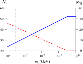
Fig. 2: Values of $N_{*}$ and $N_{\textrm{TI}}$ in our model, with $\Gamma_{\varphi}\!\ll\!H_{TI}$ and $g$, $\Gamma_{\varphi}$ and $\lambda$ values from LABEL:Table:_Free_Parameter_Values_(alpha=1_and_Gamma_{varphi}<<H_{TI}). (Plots of LABEL:Eq.:_N_(Gamma_{varphi}_<<_H_{TI}) and LABEL:Eq.:_N_{*}_(Gamma_{varphi}_<<_H_{TI}), with $m\!=\!m_{0}$.) The Blue solid line depicts $N_{*}$ and the Red dashed line depicts $N_{\rm TI}$, such that $N_{*}+N_{\rm TI}=52$. The vertical dotted line depicts values for $m_{0}=10^{3}\,$GeV.

Parameter	Value
$N_{\textrm{TI}}$	$24$
$N_{\ast}$	$28$

Table 3: Values of $N_{\textrm{TI}}$ and $N_{\ast}$ in our model, with $\Gamma_{\varphi}\!\ll\!H_{\textrm{TI}}$, $m_{0}\!\sim\!10^{3}\ \mbox{GeV}$ and $g$, $H_{\ast}$, $\Gamma_{\varphi}$ and $\lambda$ values from LABEL:Table:_Free_Parameter_Values_(alpha=1_and_Gamma_{varphi}<<H_{TI}).

The predicted values of $n_{s}$ and $n_{s}^{\prime}$ of the model for a thermal waterfall field mass of $m_{0}\!\sim\!10^{3}\ \mbox{GeV}$ in all cases of $\phi_{\ast}$ are the same to within at least four significant figures. They are also both insensitive to the value of $m_{\psi}$ within its allowed range. $n_{s}$ and $n_{s}^{\prime}$ are shown in LABEL:Table:_n_{s}_and_n_{s}'_for_m_{0}sim10^{3}(alpha=1_and_Gamma_{varphi}<<H_{TI}), with them both being within current observational bounds [2]. The prediction of the model for $n_{s}$ and $n_{s}^{\prime}$ and for a spectator field mass at the upper bound of $m_{\psi}\!=\!10^{-2}\ \mbox{GeV}$ are shown in LABEL:Figure:_n_{s}_for_phi_{*}_Case_A and LABEL:Figure:_n_{s}'_for_phi_{*}_Case_A with the parameter values of LABEL:Table:_Free_Parameter_Values_(alpha=1_and_Gamma_{varphi}<<H_{TI}).

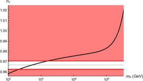
Fig. 3: Prediction of the model for $n_{s}$ with primordial inflation being quadratic chaotic inflation $\Gamma_{\varphi}\!\ll\!H_{TI}$, $m_{\psi}\!=\!10^{-2}\ \mbox{GeV}$ and the parameter values from LABEL:Table:_Free_Parameter_Values_(alpha=1_and_Gamma_{varphi}<<H_{TI}). (A plot of LABEL:Eq.:_n_{s}, irrespective of the value of $\phi_{\ast}$, with $m\!=\!m_{0}$ and $\Gamma\!=\!g^{2}m_{0}$.) The Blue and Red lines are the central value and lower/upper bounds of $n_{s}$, respectively, as obtained by the Planck mission [2].

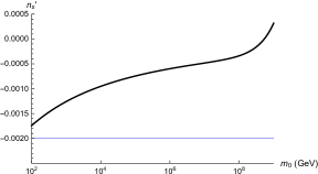
Fig. 4: Prediction of the model for $n_{s}^{\prime}$ with primordial inflation being quadratic chaotic inflation, with $\Gamma_{\varphi}\!\ll\!H_{TI}$, $m_{\psi}\!=\!10^{-2}\ \mbox{GeV}$ and the parameter values from LABEL:Table:_Free_Parameter_Values_(alpha=1_and_Gamma_{varphi}<<H_{TI}). (A plot of LABEL:Eq.:_n_{s}', irrespective of the value of $\phi_{\ast}$, with $m\!=\!m_{0}$ and $\Gamma\!=\!g^{2}m_{0}$.) The Blue line is the central value of $n_{s}^{\prime}$ as obtained by the Planck mission [2], with the lower and upper bounds being outside the displayed range of $n_{s}^{\prime}$.

Quantity	Value
$n_{s}$	$0.9645$
$n_{s}^{\prime}$	$-0.001259$

Table 4: Prediction for $n_{s}$ and $n_{s}^{\prime}$ of the model with primordial inflation being quadratic chaotic inflation, with $\Gamma_{\varphi}\!\ll\!H_{\textrm{TI}}$, $m_{\psi}\!=\!10^{-2}\ \mbox{GeV}$, $m_{0}\!\sim\!10^{3}\ \mbox{GeV}$ and the parameter values from LABEL:Table:_Free_Parameter_Values_(alpha=1_and_Gamma_{varphi}<<H_{TI}).

5 Conclusions

We have thoroughly investigated a new model of thermal inflation, where the thermal waterfall field is coupled to a spectator field, which is responsible for the observed primordial curvature perturbation through the “end of inflation” mechanism. We have derived a multitude of constraints for the model parameters. We have found that the allowed parameter space for our model corresponds to a sharp prediction for inflationary observables, like the spectral index and its running. Taking quadratic chaotic inflation as an example, we have obtained the values shown in LABEL:Table:_n_{s}_and_n_{s}'_for_m_{0}sim10^{3}(alpha=1_and_Gamma_{varphi}<<H_{TI}), which are in excellent agreement with the latest Planck data (well within 1-$\sigma$). We also found negligible tensors, with $r\sim 10^{-13}$.

Our model works with tachyonic mass for our thermal waterfall field that is of order 1 TeV. This is rather natural for a flaton field, which corresponds to a flat direction in supersymmetry lifted by a soft mass [31, 32, 33]. The energy scale of primordial and of thermal inflation were found to be $10^{13}\,$GeV and $10^{8}\,$GeV respectively, which are very reasonable values. Notice that low-scale primordial inflation ensures that the contribution to the curvature perturbation of the inflaton field is negligible.

It should be stressed that the choice of model for primordial inflation may differ from our quadratic chaotic inflation example. We have found that, in the allowed parameter space, the direct contribution of our spectator field to $n_{s}$ and $n_{s}^{\prime}$ is negligible as $\eta_{\psi}\sim 10^{-8}$. Thus, our expressions in Eqs. 3.2 and 3.11 become $n_{s}\simeq 1-2\epsilon$ and $n_{s}^{\prime}\simeq 8\epsilon^{2}+4\epsilon\eta$. Therefore, given a particular model of primordial inflation, it is straightforward to evaluate the slow-roll parameters $\epsilon$ and $\eta$ and find $n_{s}$ and $n_{s}^{\prime}$.

The number $N_{*}$ of remaining e-folds of primordial inflation when the cosmological scales exit the horizon is drastically reduced by the presence of a subsequent period of thermal inflation. In the allowed parameter space, $N_{*}\simeq 28$. This determines the values of $\epsilon$ and $\eta$ and in turn the observables $n_{s}$ and $n_{s}^{\prime}$. Note that our $N_{*}$ is substantially smaller than the usual 60 e-folds. Consequently, the produced values of $n_{s}$ and $n_{s}^{\prime}$ may vary substantially from the usual numbers corresponding to the particular model of primordial inflation considered. This can render viable inflationary models that would be otherwise excluded by observations. This effect of a period of thermal inflation resurrecting inflationary models has been employed in Ref. [34].

Note also that, in our case, thermal inflation can last much longer that the typical 10-15 e-folds, because we have considered that reheating for primordial inflation occurs after thermal inflation. So, the above effect, i.e. modifying the inflationary observables by changing $N_{*}$ due to thermal inflation, is intensified.

All in all, we have thoroughly investigated a new model of thermal inflation, in which the curvature perturbation is due to a spectator field coupled to the thermal waterfall field. For natural values of the model’s mass scales, we have found a sharp prediction of inflationary observables that depends on the chosen model of primordial inflation. Considering quadratic chaotic inflation resulted in numbers that are in excellent agreement with Planck observations. Our paper serves to remind readers that realistic models of inflation, in which the curvature perturbation is not generated by the inflaton field, are viable alternatives to the simple single-field inflation paradigm.

References

- [1] D. H. Lyth and A. R. Liddle, The Primordial Density Perturbation: Cosmology, Inflation and the Origin of Structure. Cambridge University Press, 2009.
-
[2]
Planck Collaboration,
P. A. R. Ade et al., Planck 2015 results. XIII. Cosmological parameters, Astron. Astrophys. 594 (2016) A13, arXiv:1502.01589v2 [astro-ph.CO];
P. A. R. Ade et al. [Planck Collaboration], Planck 2015 results. XX. Constraints on inflation, Astron. Astrophys. 594 (2016) A20, arXiv:1502.02114 [astro-ph.CO]. - [3] D. H. Lyth and D. Wands, Generating the curvature perturbation without an inflaton, Phys.Lett. B524 (2002) 5–14, arXiv:hep-ph/0110002v2 [hep-ph].
- [4] D. H. Lyth, C. Ungarelli and D. Wands, The Primordial density perturbation in the curvaton scenario, Phys.Rev. D67 (2003) 023503, arXiv:astro-ph/0208055v3 [astro-ph].
- [5] K.-Y. Choi and O. Seto, Modulated reheating by curvaton, Phys.Rev. D85 (2012) 123528, arXiv:1204.1419v1 [astro-ph.CO].
- [6] K. Dimopoulos, Can a vector field be responsible for the curvature perturbation in the Universe?, Phys.Rev. D74 (2006) 083502, arXiv:hep-ph/0607229v2 [hep-ph].
- [7] K. Dimopoulos, M. Karciauskas, D. H. Lyth and Y. Rodriguez, Statistical anisotropy of the curvature perturbation from vector field perturbations, JCAP 0905 (2009) 013, arXiv:0809.1055v5 [astro-ph].
-
[8]
K. Dimopoulos, Statistical Anisotropy and the Vector Curvaton Paradigm,
Int.J.Mod.Phys.
D21 (2012) 1250023,
arXiv:1107.2779v2
[hep-ph];
Erratum: Statistical Anisotropy and the Vector Curvaton Paradigm, Int.J.Mod.Phys. D21 (2012) 1292003, arXiv:1107.2779v2 [hep-ph]. - [9] S. Yokoyama and J. Soda, Primordial statistical anisotropy generated at the end of inflation, JCAP 0808 (2008) 005, arXiv:0805.4265v6 [astro-ph].
- [10] H. Assadullahi, H. Firouzjahi, M. H. Namjoo and D. Wands, Modulated curvaton decay, arXiv:1301.3439v1 [hep-th].
- [11] D. Langlois and T. Takahashi, Density Perturbations from Modulated Decay of the Curvaton, arXiv:1301.3319v1 [astro-ph.CO].
- [12] S. Enomoto, K. Kohri and T. Matsuda, Modulated decay in the multi-component Universe, arXiv:1301.3787v1 [hep-ph].
- [13] K. Kohri, C.-M. Lin and T. Matsuda, Delta-N Formalism for Curvaton with Modulated Decay, arXiv:1303.2750v1 [hep-ph].
- [14] K. Dimopoulos, G. Lazarides, D. Lyth and R. Ruiz de Austri, Curvaton dynamics, Phys.Rev. D68 (2003) 123515, arXiv:hep-ph/0308015v1 [hep-ph].
- [15] G. Dvali, A. Gruzinov and M. Zaldarriaga, New mechanism for generating density perturbations from inflation, Phys.Rev. D69 (2004) 023505, arXiv:astro-ph/0303591v1 [astro-ph].
- [16] G. Dvali, A. Gruzinov and M. Zaldarriaga, Cosmological perturbations from inhomogeneous reheating, freezeout, and mass domination, Phys.Rev. D69 (2004) 083505, arXiv:astro-ph/0305548v1 [astro-ph].
- [17] M. Postma, Inhomogeneous reheating scenario with low scale inflation and/or MSSM flat directions, JCAP 0403 (2004) 006, arXiv:astro-ph/0311563v2 [astro-ph].
- [18] F. Vernizzi, Generating cosmological perturbations with mass variations, Nucl.Phys.Proc.Suppl. 148 (2005) 120–127, arXiv:astro-ph/0503175v1 [astro-ph].
- [19] F. Vernizzi, Cosmological perturbations from varying masses and couplings, Phys.Rev. D69 (2004) 083526, arXiv:astro-ph/0311167v3 [astro-ph].
- [20] M. Kawasaki, T. Takahashi and S. Yokoyama, Density Fluctuations in Thermal Inflation and Non-Gaussianity, JCAP 0912 (2009) 012, arXiv:0910.3053v3 [hep-th].
- [21] D. H. Lyth, Generating the curvature perturbation at the end of inflation, JCAP 0511 (2005) 006, arXiv:astro-ph/0510443v3 [astro-ph].
- [22] M. P. Salem, On the generation of density perturbations at the end of inflation, Phys.Rev. D72 (2005) 123516, arXiv:astro-ph/0511146v5 [astro-ph].
- [23] L. Alabidi and D. H. Lyth, Curvature perturbation from symmetry breaking the end of inflation, JCAP 0608 (2006) 006, arXiv:astro-ph/0604569v3 [astro-ph].
- [24] D. H. Lyth, The hybrid inflation waterfall and the primordial curvature perturbation, JCAP 1205 (2012) 022, arXiv:1201.4312v4 [astro-ph.CO].
- [25] D. H. Lyth and A. Riotto, Generating the Curvature Perturbation at the End of Inflation in String Theory, Phys.Rev.Lett. 97 (2006) 121301, arXiv:astro-ph/0607326v1 [astro-ph].
- [26] M. Sasaki, Multi-brid inflation and non-Gaussianity, Prog.Theor.Phys. 120 (2008) 159–174, arXiv:0805.0974v3 [astro-ph].
- [27] F. Bernardeau, L. Kofman and J.-P. Uzan, Modulated fluctuations from hybrid inflation, Phys.Rev. D70 (2004) 083004, arXiv:astro-ph/0403315v1 [astro-ph].
- [28] T. Matsuda, Cosmological perturbations from an inhomogeneous phase transition, Class.Quant.Grav. 26 (2009) 145011, arXiv:0902.4283v3 [hep-ph].
- [29] L. Alabidi, K. Malik, C. T. Byrnes and K.-Y. Choi, How the curvaton scenario, modulated reheating and an inhomogeneous end of inflation are related, JCAP 1011 (2010) 037, arXiv:1002.1700v2 [astro-ph.CO].
- [30] D. H. Lyth and E. D. Stewart, Cosmology with a TeV mass GUT Higgs, Phys.Rev.Lett. 75 (1995) 201–204, arXiv:hep-ph/9502417v1 [hep-ph].
- [31] D. H. Lyth and E. D. Stewart, Thermal inflation and the moduli problem, Phys.Rev. D53 (1996) 1784–1798, arXiv:hep-ph/9510204v2 [hep-ph].
- [32] T. Barreiro, E. J. Copeland, D. H. Lyth and T. Prokopec, Some aspects of thermal inflation: The Finite temperature potential and topological defects, Phys.Rev. D54 (1996) 1379–1392, arXiv:hep-ph/9602263v2 [hep-ph].
- [33] T. Asaka and M. Kawasaki, Cosmological moduli problem and thermal inflation models, Phys.Rev. D60 (1999) 123509, arXiv:hep-ph/9905467v1 [hep-ph].
- [34] K. Dimopoulos and C. Owen, How Thermal Inflation can save Minimal Hybrid Inflation in Supergravity, JCAP 10 (2016) 020, arXiv:1606.06677 [hep-ph].
- [35] K. Dimopoulos and C. Owen, Modelling inflation with a power-law approach to the inflationary plateau, Phys.Rev. D94 (2016) 063518, arXiv:1607.02469 [hep-ph].
- [36] A. Rumsey, Thermal Inflation with a Thermal Waterfall Scalar Field Coupled to a Light Spectator Scalar Field. Thesis, Lancaster University, 2016. arXiv:1610.00146v1 [astro-ph.CO]. http://inspirehep.net/record/1489131/files/arXiv:1610.00146.pdf.
- [37] K. Dimopoulos and D. H. Lyth, Models of inflation liberated by the curvaton hypothesis, Phys.Rev. D69 (2004) 123509, arXiv:hep-ph/0209180 [hep-ph].
- [38] E. W. Kolb and M. S. Turner, The Early Universe, Front. Phys. 69 (1990) 1.
- [39] T. S. Bunch and P. C. W. Davies, Quantum Field Theory in de Sitter Space: Renormalization by Point Splitting, Proc. Roy. Soc. Lond. A360 (1978) 117–134.
- [40] A. A. Starobinsky and J. Yokoyama, Equilibrium state of a selfinteracting scalar field in the De Sitter background, Phys.Rev. D50 (1994) 6357, arXiv:astro-ph/9407016 [astro-ph].
- [41] A. Ashoorioon, K. Dimopoulos, M. M. Sheikh-Jabbari and G. Shiu, Reconciliation of High Energy Scale Models of Inflation with Planck, JCAP 02 (2014) 025, arXiv:1306.4914 [hep-th].