*

Abstract

We propose a novel method for semi-supervised learning (SSL) based on data-driven distributionally robust optimization (DRO) using optimal transport metrics. Our proposed method enhances generalization error by using the non-labeled data to restrict the support of the worst case distribution in our DRO formulation. We enable the implementation of our DRO formulation by proposing a stochastic gradient descent algorithm which allows to easily implement the training procedure. We demonstrate that our Semi-supervised DRO method is able to improve the generalization error over natural supervised procedures and state-of-the-art SSL estimators. Finally, we include a discussion on the large sample behavior of the optimal uncertainty region in the DRO formulation. Our discussion exposes important aspects such as the role of dimension reduction in SSL.

1 Introduction

We propose a novel method for semi-supervised learning (SSL) based on data-driven distributionally robust optimization (DRO) using an optimal transport metric – also known as earth-moving distance (see [19]).

Our approach enhances generalization error by using the unlabeled data to restrict the support of the models which lie in the region of distributional uncertainty. The intuition is that our mechanism for fitting the underlying model is automatically tuned to generalize beyond the training set, but only over potential instances which are relevant. The expectation is that predictive variables often lie in lower dimensional manifolds embedded in the underlying ambient space; thus, the shape of this manifold is informed by the unlabeled data set (see Figure 1 for an illustration of this intuition).

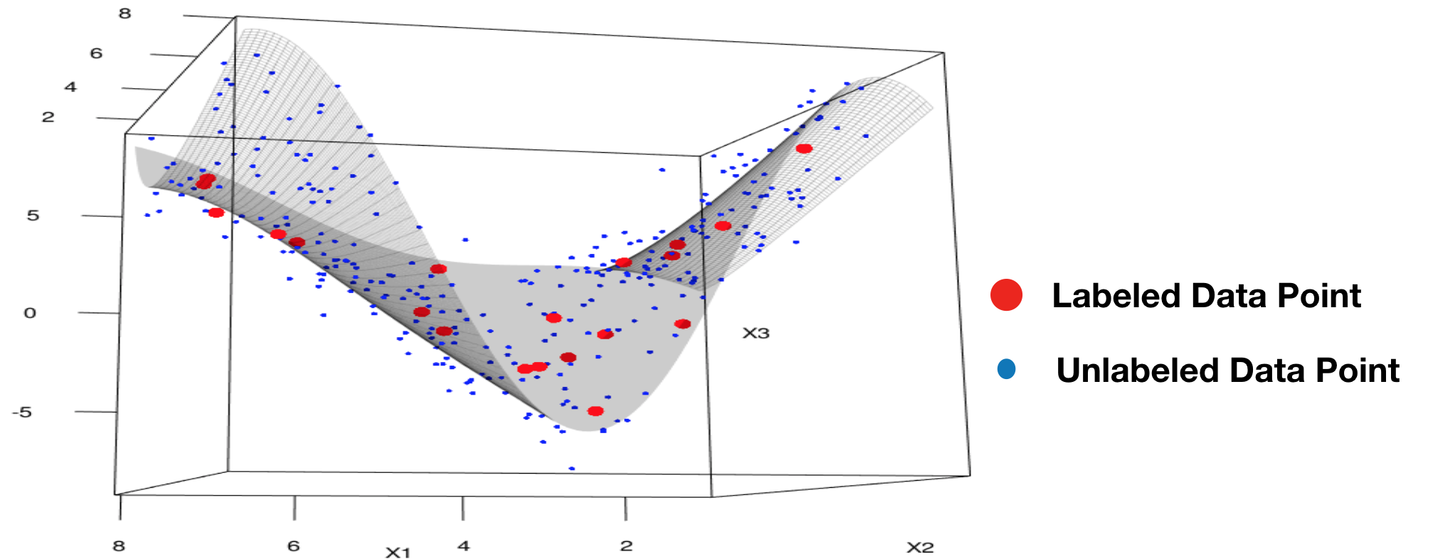
Figure 1: Idealization of the way in which the unlabeled predictive variables provide a proxy for an underlying lower dimensional manifold. Large red dots represent labeled instances and small blue dots represent unlabeled instances.

To enable the implementation of the DRO formulation we propose a stochastic gradient descent (SGD) algorithm which allows to implement the training procedure at ease. Our SGD construction includes a procedure of independent interest which, we believe, can be used in more general stochastic optimization problems.

We focus our discussion on semi-supervised classification but the modeling and computational approach that we propose can be applied more broadly as we shall illustrate in Section 4.

We now explain briefly the formulation of our learning procedure. Suppose that the training set is given by $\mathcal{D}_{n}=\{\left(Y_{i},X_{i}\right)\}_{i=1}^{n}$, where $Y_{i}\in\{-1,1\}$ is the label of the $i$-th observation and we assume that the predictive variable, $X_{i}$, takes values in $\mathbb{R}^{d}$. We use $n$ to denote the number of labeled data points.

In addition, we consider a set of unlabeled observations, $\left\{X_{i}\right\}_{i=n+1}^{N}$. We build the set $\mathcal{E}_{N-n}=\{\left(1,X_{i}\right)\}_{i=n+1}^{N}\cup\{\left(-1,X_{i}\right)\}_{i=n+1}^{N}$. That is, we replicate each unlabeled data point twice, recognizing that the missing label could be any of the two available alternatives. We assume that the data must be labeled either -1 or 1.

We then construct the set $\mathcal{X}_{N}=\mathcal{D}_{n}\cup\mathcal{E}_{N-n}$ which, in simple words, is obtained by just combining both the labeled data and the unlabeled data with all the possible labels that can be assigned. The cardinality of $\mathcal{X}_{N}$, denoted as $\left|\mathcal{X}_{N}\right|$, is equal to $2\left(N-n\right)+n$ (for simplicity we assume that all of the data points and the unlabeled observations are distinct).

Let us define $\mathcal{P}\left(\mathcal{X}_{N}\right)$ to be the space of probability measures whose support is contained in $\mathcal{X}_{N}$. We use $P_{n}$ to denote the empirical measure supported on the set $\mathcal{D}_{n}$, so $P_{n}\in\mathcal{P}\left(\mathcal{X}_{N}\right)$. In addition, we write $E_{P}\left(\cdot\right)$ to denote the expectation associated with a given probability measure $P$.

Let us assume that we are interested in fitting a classification model by minimizing a given expected loss function $l\left(X,Y,\beta\right)$, where $\beta$ is a parameter which uniquely characterizes the underlying model. We shall assume that $l\left(X,Y,\cdot\right)$ is a convex function for each fixed $\left(X,Y\right)$.  The empirical risk associated to the parameter $\beta$ is

$$E_{P_{n}}\left(l\left(X,Y,\beta\right)\right)=\frac{1}{n}\sum_{i=1}^{n}l\left(X_{i},Y_{i},\beta\right).$$

In this paper, we propose to estimate $\beta$ by solving the DRO problem

$$\min_{\beta}\max_{P\in\mathcal{P}\left(\mathcal{X}_{N}\right):D_{c}\left(P,P_{n}\right)\leq\delta^{\ast}}E_{P}[l\left(X,Y,\beta\right)],$$ (1)

where $D_{c}\left(\cdot\right)$ is a suitably defined discrepancy between $P_{n}$ and any probability measure $P\in\mathcal{P}\left(\mathcal{X}_{N}\right)$ which is within a certain tolerance measured by $\delta^{\ast}$.

So, intuitively, (1) represents the value of a game in which the outer player (we) will choose $\beta$ and the adversary player (nature) will rearrange the support and the mass of $P_{n}$ within a budget measured by $\delta^{\ast}$. We then wish to minimize the expected risk regardless of the way in which the adversary might corrupt (within the prescribed budget) the existing evidence. In formulation (1), the adversary is crucial to ensure that we endow our mechanism for selecting $\beta$ with the ability to cope with the risk impact of out-of-sample (i.e. out of the training set) scenarios. We denote the formulation in (1) as semi-supervised distributionally robust optimization (SSL-DRO).

The criterion that we use to define $D_{c}\left(\cdot\right)$ is based on the theory of optimal transport and it is closely related to the concept of Wasserstein distance, see Section 3. The choice of $D_{c}\left(\cdot\right)$ is motivated by recent results which show that popular estimators such as regularized logistic regression, Support Vector Machines (SVMs) and square-root Lasso (SR-Lasso) admit a DRO representation exactly equal to (1) in which the support $\mathcal{X}_{N}$ is replaced by $\mathbb{R}^{d+1}$ (see [6] and also equation (9) in this paper.)

In view of these representation results for supervised learning algorithms, the inclusion of $\mathcal{X}_{N}$ in our DRO formulation (1) provides a natural SSL approach in the context of classification and regression. The goal of this paper is to enable the use of the distributionally robust training framework (1) as a SSL technique. We will show that estimating $\beta$ via (1) may result in a significant improvement in generalization relative to natural supervised learning counterparts (such as regularized logistic regression and SR-Lasso). The potential improvement is illustrated in Section 4. Moreover, we show via numerical experiments in Section 5, that our method is able to improve upon state-of-the-art SSL algorithms.

As a contribution of independent interest, we construct a stochastic gradient descent algorithm to approximate the optimal selection, $\beta_{N}^{\ast}$, minimizing (1).

An important parameter when applying (1) is the size of the uncertainty region, which is parameterized by $\delta^{\ast}$. We apply cross-validation to calibrate $\delta^{\ast}$, but we also discuss the non-parametric behavior of an optimal selection of $\delta^{\ast}$ (according to a suitably defined optimality criterion explained in Section 6) as $n,N\rightarrow\infty$.

In Section 2, we provide a broad overview of alternative procedures in the SSL literature, including recent approaches which are related to robust optimization. A key role in our formulation is played by $\delta^{\ast}$, which can be seen as a regularization parameter. This identification is highlighted in the form of (1) and the DRO representation of regularized logistic regression which we recall in (9). The optimal choice of $\delta^{\ast}$ ensures statistical consistency as $n,N\rightarrow\infty$.

Similar robust optimization formulations to (1) for machine learning have been investigated in the literature recently. For example, connections between robust optimization and machine learning procedures such as Lasso and SVMs have been studied in the literature, see [23]. In contrast to this literature, the use of distributionally robust uncertainty allows to discuss the optimal size of the uncertainty region as the sample size increases (as we shall explain in Section 6). The work of [20] is among the first to study DRO representations based on optimal transport, they do not study the implications of these types of DRO formulations in SSL as we do here.

We close this Introduction with a few important notes. First, our SSL-DRO is not a robustifying procedure for a given SSL algorithm. Instead, our contribution is in showing how to use unlabeled information on top of DRO to enhance traditional supervised learning methods. In addition, our SSL-DRO formulation, as stated in (1) , is not restricted to logistic regression, instead DRO counterpart could be formulated for general supervised learning methods with various choice of loss function.

2 Alternative Semi-Supervised Learning Procedures

We shall briefly discuss alternative procedures which are known in the SSL literature, which are quite substantial. We refer the reader to the excellent survey of [24] for a general overview of the area. Our goal here is to expose the similarities and connections between our approach and some of the methods that have been adopted in the community.

For example, broadly speaking graph-based methods [7] and [9] attempt to construct a graph which represents a sketch of a lower dimensional manifold in which the predictive variables lie. Once the graph is constructed, a regularization procedure is performed, which seeks to enhance generalization error along the manifold while ensuring continuity in the prediction regarding an intrinsic metric. Our approach bypasses the construction of the graph, which we see as a significant advantage of our procedure. However, we believe that the construction of the graph can be used to inform the choice of cost function $c\left(\cdot\right)$ which should reflect high transportation costs for moving mass away from the manifold sketched by the graph.

Some recent SSL estimators are based on robust optimization, such as the work of [1]. The difference between data-driven DRO and robust optimization is that the inner maximization in (1) for robust optimization is not over probability models which are variations of the empirical distribution. Instead, in robust optimization, one attempts to minimize the risk of the worst case performance of potential outcomes inside a given uncertainty set.

In [1], the robust uncertainty set is defined in terms of constraints obtained from the testing set. The problem with the approach in [1] is that there is no clear mechanism which informs an optimal size of the uncertainty set (which in our case is parameterized by $\delta^{\ast}$). In fact, in the last paragraph of Section 2.3, [1] point out that the size of the uncertainty could have a significant detrimental impact in practical performance.

We conclude with a short discussion on the work of [14], which is related to our approach. In the context of linear discriminant analysis, [14] also proposes a distributionally robust optimization estimator, although completely different from the one we propose here. More importantly, we provide a way (both in theory and practice) to study the optimal size of the distributional uncertainty (i.e. $\delta^{\ast}$), which allows us to achieve asymptotic consistency of our estimator.

3 Semi-supervised Learning based on DRO

This section is divided into two parts. First, we provide the elements of our DRO formulation. Then we will explain how to solve the SSL-DRO problem, i.e. find optimal $\beta$ in (1).

3.1 Defining the optimal transport discrepancy:

Assume that the cost function $c:\mathbb{R}^{d+1}\times\mathbb{R}^{d+1}\rightarrow[0,\infty]$ is lower semi-continuous. As mentioned in the Introduction, we also assume that $c(u,v)=0$ if and only if $u=v$.

Now, given two distributions $P$ and $Q$, with supports $\mathcal{S}_{P}\subseteq\mathcal{X}_{N}$ and $\mathcal{S}_{Q}\subseteq\mathcal{X}_{N}$, respectively, we define the optimal transport discrepancy, $D_{c}$, via

$$D_{c}\left(P,Q\right)=\inf\{E_{\pi}\left[c\left(U,V\right)\right]:\pi\in\mathcal{P}\left(\mathcal{S}_{P}\times\mathcal{S}_{Q}\right),\text{ }\pi_{U}=P,\text{ }\pi_{V}=Q\},$$ (2)

where $\mathcal{P}\left(\mathcal{S}_{P}\times\mathcal{S}_{Q}\right)$ is the set of probability distributions $\pi$ supported on $\mathcal{S}_{P}\times\mathcal{S}_{Q}$, and $\pi_{U}$ and $\pi_{V}$ denote the marginals of $U$ and $V$ under $\pi$, respectively.

If, in addition, $c\left(\cdot\right)$ is symmetric (i.e. $c\left(u,v\right)=c\left(v,u\right)$), and there exists $\varrho\geq 1$ such that $c^{1/\varrho}\left(u,w\right)\leq c^{1/\varrho}\left(u,v\right)+c^{1/\varrho}\left(v,w\right)$ (i.e. $c^{1/\varrho}\left(\cdot\right)$ satisfies the triangle inequality), it can be easily verified (see [22]) that $D_{c}^{1/\varrho}\left(P,Q\right)$ is a metric. For example, if $c\left(u,v\right)=\left\|u-v\right\|_{q}^{\varrho}$ for $q\geq 1$ (where $\left\|u-v\right\|_{q}$ denotes the $l_{q}$ norm in $\mathbb{R}^{d+1}$) then $D_{c}\left(\cdot\right)$ is known as the Wasserstein distance of order $\varrho$.

Observe that (2) is obtained by solving a linear programming problem. For example, suppose that $Q=P_{n}$, and let $P\in\mathcal{P}\left(\mathcal{X}_{N}\right)$ then, using $U=\left(X,Y\right)$, we have that $D_{c}\left(P,P_{n}\right)$ is obtained by computing

$$\min_{\pi}\big{\{} \sum_{u\in\mathcal{X}_{N}}\sum_{v\in\mathcal{D}_{n}}c\left(u,v\right)\pi\left(u,v\right):\mbox{ s.t.}\sum_{u\in\mathcal{X}_{N}}\pi\left(u,v\right)=\frac{1}{n}\text{ }\forall\text{ }v\in\mathcal{D}_{n},$$ (3)

$$\sum_{v\in\mathcal{D}_{N}}\pi\left(u,v\right)=P\left(\left\{u\right\}\right)\text{ }\forall\text{ }u\in\mathcal{X}_{N},\pi\left(u,v\right)\geq 0\text{ }\forall\text{ }\left(u,v\right)\in\mathcal{X}_{N}\times\mathcal{D}_{n}\big{\}}$$

We shall discuss, for instance, how the choice of $c\left(\cdot\right)$ in formulations such as (1) can be used to recover popular machine learning algorithms.

3.2 Solving the SSL-DRO formulation:

A direct approach to solve (1) would involve alternating between minimization over $\beta$, which can be performed by, for example, stochastic gradient descent and maximization which is performed by solving a linear program similar to (3). Unfortunately, the large scale of the linear programming problem, which has $O(N)$ variables and $O(n)$ constraints, makes this direct approach rather difficult to apply in practice.
So, our goal here is to develop a direct stochastic gradient descent approach which can be used to approximate the solution to (1).
First, it is useful to apply linear programming duality to simplify (1). Note that, given $\beta$, the inner maximization in (1) is simply

$$\max_{\pi}\big{\{} \sum_{u\in\mathcal{X}_{N}}\sum_{v\in\mathcal{D}_{N}}l\left(u,\beta\right)\pi\left(u,v\right):\mbox{ s.t.}\sum_{u\in\mathcal{X}_{N}}\pi\left(u,v\right)=\frac{1}{n}\text{ }\forall\text{ }v\in\mathcal{D}_{n}$$ (4)

$$\sum_{u\in\mathcal{X}_{N}}\sum_{v\in\mathcal{D}_{n}}c\left(u,v\right)\pi\left(u,v\right)\leq\delta,\pi\left(u,v\right)\geq 0\text{ }\forall\text{ }\left(u,v\right)\in\mathcal{X}_{N}\times\mathcal{D}_{n}\big{\}}.$$

Of course, the feasible region in this linear program is always non-empty because the probability distribution $\pi\left(u,v\right)=I\left(u=v\right)I\left(v\in\mathcal{D}_{n}\right)/n$ is a feasible choice. Also, the feasible region is clearly compact, so the dual problem is always feasible and by strong duality its optimal value coincides with that of the primal problem, see [2, 3, 6]. The dual problem associated to (4) is given by

$$\min\big{\{}\sum_{v\in\mathcal{D}_{N}}\gamma\left(v\right)/n+\lambda\delta\text{ s.t. } \gamma\left(v\right)\in\mathbb{R}\text{ }\forall\text{ }v\in\mathcal{D}_{n}\text{, }\lambda\geq 0,$$ (5)

$$\gamma\left(v\right)\geq l\left(u,\beta\right)-\lambda c\left(u,v\right)\text{ }\forall\text{ }\left(u,v\right)\in\mathcal{X}_{N}\times\mathcal{D}_{n}.\big{\}}$$

Maximizing over $u\in\mathcal{X}_{N}$ in the inequality constraint, for each $v$, and using the fact that we are minimizing the objective function, we obtain that (5) can be simplified to

$$\left.E_{P_{n}}[\max_{u\in\mathcal{X}_{N}}\left\{l\left(u,\beta\right)-\lambda c\left(u,\left(X,Y\right)\right)+\lambda\delta^{\ast}\right\}]\right..$$

Consequently, defining $\phi\left(X,Y,\beta,\lambda\right)=\max_{u\in\mathcal{X}_{N}}\left\{l\left(u,\beta\right)-\lambda c\left(u,\left(X,Y\right)\right)+\lambda\delta^{\ast}\right\}$, we have that (1) is equivalent to

$$\min_{\lambda\geq 0,\beta}\left.E_{P_{n}}[\phi\left(X,Y,\beta,\lambda\right)]\right..$$ (6)

Moreover, if we assume that $l\left(u,\cdot\right)$ is a convex function, then we have that the mapping $\left(\beta,\lambda\right)\hookrightarrow l\left(u,\beta\right)-\lambda c\left(u,\left(X,Y\right)\right)+\lambda\delta^{\ast}$is convex for each $u$ and therefore, $\left(\beta,\lambda\right)\hookrightarrow\phi\left(X,Y,\beta,\lambda\right)$, being the maximum of convex mappings is also convex.

A natural approach consists in directly applying stochastic sub-gradient descent (see [8] and [17]). Unfortunately, this would involve performing the maximization over all $u\in\mathcal{X}_{N}$ in each iteration. This approach could be prohibitively expensive in typical machine learning applications where $N$ is large.

So, instead, we perform a standard smoothing technique, namely, we introduce $\epsilon>0$ and define

$$\phi_{\epsilon}\left(X,Y,\beta,\lambda\right)=\lambda\delta^{\ast}+\epsilon\log\big{(}\sum_{u\in\mathcal{X}_{N}}\exp\left(\left\{l\left(u,\beta\right)-\lambda c\left(u,\left(X,Y\right)\right)\right\}/\epsilon\right)\big{)}.$$

It is easy to verify (using Hölder inequality) that $\phi_{\epsilon}\left(X,Y,\cdot\right)$ is convex and it also follows that

$$\phi\left(X,Y,\beta,\lambda\right)\leq\phi_{\epsilon}\left(X,Y,\beta,\lambda\right)\leq\phi\left(X,Y,\beta,\lambda\right)+\log(\left|\mathcal{X}_{N}\right|)\epsilon.$$

Hence, we can choose $\epsilon=O\left(1/\log N\right)$ in order to control the bias incurred by replacing $\phi$ by $\phi_{\epsilon}$. Then, defining

$$\tau_{\epsilon}\left(X,Y,\beta,\lambda,u\right)=\exp\left(\left\{l\left(u,\beta\right)-\lambda c\left(u,\left(X,Y\right)\right)\right\}/\epsilon\right),$$

we have (assuming differentiability of $l\left(u,\beta\right)$) that

$$\nabla_{\beta}\phi_{\epsilon}\left(X,Y,\beta,\lambda\right)=\quad\quad\quad\frac{\sum_{u\in\mathcal{X}_{N}}\tau_{\epsilon}\left(X,Y,\beta,\lambda,u\right)\nabla_{\beta}l\left(u,\beta\right)}{\sum_{v\in\mathcal{X}_{N}}\tau_{\epsilon}\left(X,Y,\beta,\lambda,v\right)},$$ (7)

$$\frac{\partial\phi_{\epsilon}\left(X,Y,\beta,\lambda\right)}{\partial\lambda}=\quad\quad\delta^{\ast}-\frac{\sum_{u\in\mathcal{X}_{N}}\tau_{\epsilon}\left(X,Y,\beta,\lambda,u\right)c\left(u,\left(X,Y\right)\right)}{\sum_{v\in\mathcal{X}_{N}}\tau_{\epsilon}\left(X,Y,\beta,\lambda,v\right)}.$$

In order to make use of the gradient representations (7) for the construction of a stochastic gradient descent algorithm, we must construct unbiased estimators for $\nabla_{\beta}\phi_{\epsilon}\left(X,Y,\beta,\lambda\right)$ and $\partial\phi_{\epsilon}\left(X,Y,\beta,\lambda\right)/\partial\lambda$, given $\left(X,Y\right)$. This can be easily done if we assume that one can simulate directly $u\in\mathcal{X}_{N}$ with probability proportional to $\tau\left(X,Y,\beta,\lambda,u\right)$. Because of the potential size of $\mathcal{X}_{N}$ and especially because such distribution depends on $\left(X,Y\right)$ sampling with probability proportional to $\tau_{\epsilon}\left(X,Y,\beta,\lambda,u\right)$ can be very time-consuming.

So, instead, we apply a strategy discussed in [4] and explained in Section 2.2.1. The proposed method produces random variables $\Lambda\left(X,Y,\beta,\lambda\right)$ and $\Gamma\left(X,Y,\beta,\lambda\right)$, which can be simulated easily by drawing i.i.d. samples from the uniform distribution over $\mathcal{X}_{N}$, and such that

$$E\left(\Lambda\left(X,Y,\beta,\lambda\right)|X,Y\right)={\partial_{\lambda}}\phi_{\epsilon}\left(X,Y,\beta,\lambda\right),$$

$$E\left(\Gamma\left(X,Y,\beta,\lambda\right)|X,Y\right)=\nabla_{\beta}\phi_{\epsilon}\left(X,Y,\beta,\lambda\right).$$

Using this pair of random variables, then we apply the stochastic gradient descent recursion

$$\beta_{k+1}=\beta_{k}-\alpha_{k+1}\Gamma\left(X_{k+1},Y_{k+1},\beta_{k},\lambda_{k}\right),$$

$$\lambda_{k+1}=\left(\lambda_{k}-\alpha_{k+1}\Lambda\left(X_{k+1},Y_{k+1},\beta_{k},\lambda_{k}\right)\right)^{+},$$ (8)

where learning sequence, $\alpha_{k}>0$ satisfies the standard conditions, namely, $\sum_{k=1}^{\infty}\alpha_{k}=\infty$ and $\sum_{k=1}^{\infty}\alpha_{k}^{2}<\infty$, see [21].

We apply a technique from [4] to construct the random variables $\Lambda$ and $\Gamma$, which originates from Multilevel Monte Carlo introduced in [10], and associated randomization methods [16],[18].

First, define $\bar{P}_{N}$ to be the uniform measure on $\mathcal{X}_{N}$ and let $W$ be a random variable with distribution $\bar{P}_{N}$. Note that, given $\left(X,Y\right)$,

$$\nabla_{\beta}\phi_{\epsilon}\left(X,Y,\beta,\lambda\right)=\frac{E_{\bar{P}_{N}}\left(\tau_{\epsilon}\left(X,Y,\beta,\lambda,W\right)\nabla_{\beta}l\left(W,\beta\right)|\text{ }X,Y\right)}{E_{\bar{P}_{N}}\left(\tau_{\epsilon}\left(X,Y,\beta,\lambda,W\right)|\text{ }X,Y\right)},$$

$$\partial_{\lambda}\phi_{\epsilon}\left(X,Y,\beta,\lambda\right)=\quad\delta^{\ast}-\frac{E_{\bar{P}_{N}}\left(\tau_{\epsilon}\left(X,Y,\beta,\lambda,W\right)c\left(W,\left(X,Y\right)\right)|\text{ }X,Y\right)}{E_{\bar{P}_{N}}\left(\tau_{\epsilon}\left(X,Y,\beta,\lambda,W\right)|\text{ }X,Y\right)}.$$

Note that both gradients can be written in terms of the ratios of two expectations. The following results from [4] can be used to construct unbiased estimators of functions of expectations. The function of interest in our case is the ratio of expectations.

Let us define: $h_{0}\left(W\right)=\tau_{\epsilon}\left(X,Y,\beta,\lambda,W\right)$, $h_{1}\left(W\right)=h_{0}\left(W\right)c\left(W,\left(X,Y\right)\right)$ , and $h_{2}\left(W\right)=h_{0}\left(W\right)\nabla_{\beta}l\left(W,\beta\right)$, Then, we can write the gradient estimator as

$$\partial_{\lambda}\phi_{\epsilon}\left(X,Y,\beta,\lambda\right)=\frac{E_{\bar{P}_{N}}\left(h_{1}\left(W\right)\text{ }|\text{ }X,Y\right)}{E_{\bar{P}_{N}}\left(h_{0}\left(W\right)\text{ }|\text{ }X,Y\right)},$$

$$\text{ and }\nabla_{\beta}\phi_{\epsilon}\left(X,Y,\beta,\lambda\right)=\frac{E_{\bar{P}_{N}}\left(h_{2}\left(W\right)\text{ }|\text{ }X,Y\right)}{E_{\bar{P}_{N}}\left(h_{0}\left(W\right)\text{ }|\text{ }X,Y\right)}.$$

The procedure developed in [4] proceeds as follows. First, define for a given $h\left(W\right)$, and $n\geq 0$, the average over odd and even labels to be

$$\bar{S}_{2^{n}}^{E}\left(h\right)=\frac{1}{2^{n}}\sum_{i=1}^{2^{n}}h\left(W_{2i}\right),\text{ \ }\bar{S}_{2^{n}}^{O}\left(h\right)=\frac{1}{2^{n}}\sum_{i=1}^{2^{n}}h\left(W_{2i-1}\right),$$

and the total average to be $\bar{S}_{2^{n+1}}\left(h\right)=\frac{1}{2}\left(\bar{S}_{2^{n}}^{E}\left(h\right)+\bar{S}_{2^{n}}^{O}\left(h\right)\right)$. We then state the following algorithm for sampling unbiased estimators of $\partial_{\lambda}\phi_{\epsilon}\left(X,Y,\beta,\lambda\right)$ and $\nabla_{\beta}\phi_{\epsilon}\left(X,Y,\beta,\lambda\right)$ in Algorithm 1.

Algorithm 1 Unbiased Gradient

1:Given $\left(X,Y,\beta\right)$ the function outputs $\left(\Lambda,\Gamma\right)$ such that $E\left(\Lambda\right)=\partial_{\lambda}\phi_{\epsilon}\left(X,Y,\beta,\lambda\right)$ and $E\left(\Gamma\right)=\nabla_{\beta}\phi_{\epsilon}\left(X,Y,\beta,\lambda\right)$.

2:Step1: Sample $G$ from geometric distribution with success parameter $p_{G}=1-2^{-3/2}$.

3:Step2: Sample $W_{0},W_{1},...,W_{2^{G+1}}$ i.i.d. copies of $W$ independent of $G$.

4:Step3: Compute

$$\Delta^{\lambda} =\frac{\bar{S}_{2^{G+1}}\left(h_{1}\right)}{\bar{S}_{2^{G+1}}\left(h_{0}\right)}-\frac{1}{2}\left(\frac{\bar{S}_{2^{G+1}}^{O}\left(h_{1}\right)}{\bar{S}_{2^{G+1}}^{O}\left(h_{0}\right)}+\frac{\bar{S}_{2^{G}}^{E}\left(h_{1}\right)}{\bar{S}_{2^{G}}^{E}\left(h_{0}\right)}\right),$$

$$\Delta^{\beta} =\frac{\bar{S}_{2^{G+1}}\left(h_{2}\right)}{\bar{S}_{2^{G+1}}\left(h_{0}\right)}-\frac{1}{2}\left(\frac{\bar{S}_{2^{G+1}}^{O}\left(h_{2}\right)}{\bar{S}_{2^{G+1}}^{O}\left(h_{0}\right)}+\frac{\bar{S}_{2^{G}}^{E}\left(h_{2}\right)}{\bar{S}_{2^{G}}^{E}\left(h_{0}\right)}\right).$$

5:Output:

$$\Lambda=\delta^{\ast}-\frac{\Delta^{\lambda}}{p_{G}\left(1-p_{G}\right)^{G}}-\frac{h_{1}\left(W_{0}\right)}{h_{0}\left(W_{0}\right)},\qquad\Gamma=\frac{\Delta^{\beta}}{p_{G}\left(1-p_{G}\right)^{G}}+\frac{h_{2}\left(W_{0}\right)}{h_{0}\left(W_{0}\right)}.$$

4 Error Improvement of Our SSL-DRO Formulation

Our goal in this section is to intuitively discuss why, owing to the inclusion of the constraint $P\in\mathcal{P}\left(\mathcal{X}_{N}\right)$, we expect desirable generalization properties of the SSL-DRO formulation (1). Moreover, our intuition suggests strongly why our SSL-DRO formulation should possess better generalization performance than natural supervised counterparts. We restrict the discussion for logistic regression due to the simple form of regularization connection we will make in (9), however, the error improvement discussion should also apply to general supervised learning setting.

As discussed in the Introduction using the game-theoretic interpretation of (1), by introducing $\mathcal{P}\left(\mathcal{X}_{N}\right)$, the SSL-DRO formulation provides a mechanism for choosing $\beta$ which focuses on potential out-of-sample scenarios which are more relevant based on available evidence.

Suppose that the constraint $P\in\mathcal{P}\left(\mathcal{X}_{N}\right)$ was not present in the formulation. So, the inner maximization in (1) is performed over all probability measures $\mathcal{P}\left(\mathbb{R}^{d+1}\right)$ (supported on some subset of $\mathbb{R}^{d+1}$). As indicated earlier, we assume that $l\left(X,Y;\cdot\right)$ is strictly convex and differentiable, so the first order optimality condition $E_{P}\left(\nabla_{\beta}l\left(X,Y;\beta\right)\right)=0$ characterizes the optimal choice of $\beta$ assuming the validity of the probabilistic model $P$. It is natural to assume that there exists an actual model underlying the generation of the training data, which we denote as $P_{\infty}$. Moreover, we may also assume that there exists a unique $\beta^{\ast}$ such that $E_{P_{\infty}}\left(\nabla_{\beta}l\left(X,Y;\beta^{\ast}\right)\right)=0$.

The set $\mathcal{M}\left(\beta_{\ast}\right)=\mathcal{\{}P\in\mathcal{P}\left(\mathbb{R}^{d+1}\right):E_{P}\left(\nabla_{\beta}l\left(X,Y;\beta^{\ast}\right)\right)=0\mathcal{\}}$ corresponds to the family of all probability models which correctly estimate $\beta^{\ast}$. Clearly, $P_{\infty}\in\mathcal{M}\left(\beta_{\ast}\right)$, whereas, typically, $P_{n}\notin\mathcal{M}\left(\beta_{\ast}\right)$. Moreover, if we write $\mathcal{X}_{\infty}=$ $supp\left(P_{\infty}\right)$ we have that

$$P_{\infty}\in m\left(N,\beta^{\ast}\right):=\mathcal{\{}P\in\mathcal{P}\left(\mathcal{X}_{\infty}\right):\quad E_{P}\left(\nabla_{\beta}l\left(X,Y;\beta^{\ast}\right)\right)=0\mathcal{\}\subset M}\left(\beta_{\ast}\right).$$

Since $\mathcal{X}_{N}$ provides a sketch of $\mathcal{X}_{\infty}$, then we expect to have that the extremal (i.e. worst case) measure, denoted by $P_{N}^{\ast}$, will be in some sense a better description of $P_{\infty}$.

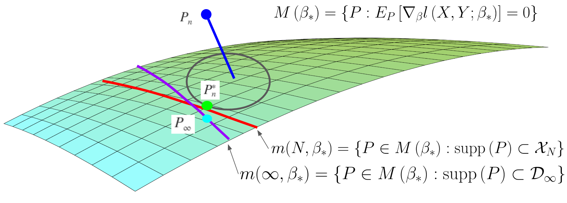
-̌0.2in

Figure 2: Pictorial representation of the role that the support constraint plays in the SSL-DRO approach and how its presence enhances the out-of-sample performance.

Figure 2 provides a pictorial representation of the previous discussion. In the absence of the constraint $P\in\mathcal{P}\left(\mathcal{X}_{N}\right)$, the extremal measure chosen by nature can be interpreted as a projection of $P_{n}$ onto $\mathcal{M}\left(\beta_{\ast}\right)$. In the presence of the constraint $P\in\mathcal{P}\left(\mathcal{X}_{N}\right)$, we can see that $P_{N}^{\ast}$ may bring the learning procedure closer to $P_{\infty}$. Of course, if $N$ is not large enough, the schematic may not be valid because one may actually have $m\left(N,\beta^{\ast}\right)=\varnothing$.

The previous discussion is useful to argue that our SSL-DRO formulation should be superior to the DRO formulation which is not informed by the unlabeled data. But this comparison may not directly apply to alternative supervised procedures that are mainstream in machine learning, which should be considered as the natural benchmark to compare with. Fortunately, replacing the constraint that $P\in\mathcal{P}\left(\mathcal{X}_{N}\right)$ by $P\in\mathcal{P}\left(\mathbb{R}^{d+1}\right)$ in the DRO formulation recovers exactly supervised learning algorithms such as regularized logistic regression.

Recall from [6] that if $l\left(x,y,\beta\right)=\log(1+\exp(-y\cdot\beta^{T}x))$ and if we define

$$c\left((x,y),(x^{\prime},y^{\prime})\right)=\|x-x^{\prime}\|_{q}I(y=y^{\prime})+\infty I(y\neq y^{\prime}),$$

for $q\geq 1$ then, according to Theorem 3 in [6], we have that

$$\min_{\beta}\max_{D_{c}\left(P,P_{n}\right)\leq\bar{\delta}}E_{P}[l\left(X,Y,\beta\right)]=\min_{\beta\in\mathbb{R}^{d}}\left\{E_{P_{n}}\left[l\left(X,Y,\beta\right)\right]+\bar{\delta}\left\|\beta\right\|_{p}\right\},$$ (9)

where $q$ satisfies $1/p+1/q=1$. Formulation (1) is, therefore, the natural SSL extension of the standard regularized logistic regression estimator.

We conclude that, for logistic regression, SSL-DRO as formulated in (1), is a natural SSL extension of the standard regularized logistic regression estimator, which would typically induce superior generalization abilities over its supervised counterparts, and similar discussion should apply to most supervised learning methods.

5 Numerical Experiments

We proceed to numerical experiments to verify the performance of our SSL-DRO method empirically using six binary classification real data sets from UCI machine learning data base [13].

We consider our SSL-DRO formulation based on logistic regression and compare with other state-of-the-art logistic regression based SSL algorithms, entropy regularized logistic regression with $L_{1}$ regulation (ERLRL1) [11] and regularized logistic regression based self-training (STLRL1) [12]. In addition, we also compare with its supervised counterpart, which is regularized logistic regression (LRL1). For each iteration of a data set, we randomly split the data into labeled training, unlabeled training and testing set, we train the models on training sets and evaluate the testing error and accuracy with testing set. We report the mean and standard deviation for training and testing error using log-exponential loss and the average testing accuracy, which are calculated via $200$ independent experiments for each data set. We summarize the detailed results, the basic information of the data sets, and our data split setting in Table 1.

We can observe that our SSL-DRO method has the potential to improve upon these state-of-the-art SSL algorithms.

		Breast Cancer	qsar	Magic	Minibone	Spambase
LRL1	Train	$.185\pm.123$	$.614\pm.038$	$.548\pm.087$	$.401\pm.167$	$.470\pm.040$
	Test	$.428\pm.338$	$.755\pm.019$	$.610\pm.050$	$.910\pm.131$	$.588\pm.141$
	Accur	$.929\pm.023$	$.646\pm.036$	$.665\pm.045$	$.717\pm.041$	$.811\pm.034$
ERLRL1	Train	$.019\pm.010$	$.249\pm.050$	$2.37\pm.987$	$.726\pm.353$	$.008\pm.028$
	Test	$.265\pm.146$	$.720\pm.029$	$4.28\pm 1.51$	$1.98\pm.678$	$.505\pm.108$
	Accur	$.944\pm.018$	$.731\pm.026$	$.721\pm.056$	$.708\pm.071$	$.883\pm.018$
STLRL1	Train	$.089\pm.019$	$.498\pm.120$	$3.05\pm.987$	$1.50\pm.706$	$.370\pm.082$
	Test	$.672\pm.034$	$2.37\pm.860$	$8.03\pm 1.51$	$4.81\pm.732$	$1.47\pm.316$
	Accur	$.955\pm.023$	$.694\pm.038$	$.692\pm.056$	$.704\pm.033$	$.843\pm.023$
DROSSL	Train	$.045\pm.023$	$.402\pm.039$	$.420\pm.075$	$.287\pm.047$	$.221\pm.028$
	Test	$.120\pm.029$	$.555\pm.025$	$.561\pm.039$	$.609\pm.054$	$.333\pm.012$
	Accur	$.956\pm.016$	$.734\pm.025$	$.733\pm.034$	$.710\pm.032$	$.892\pm.009$
Num Predictors		$30$	$30$	$10$	$20$	$56$
Labeled Size		$40$	$80$	$30$	$30$	$150$
Unlabeled Size		$200$	$500$	$9000$	$5000$	$1500$
Testing Size		$329$	$475$	$9990$	$125034$	$2951$

Table 1: Numerical experiments for real data sets.

6 Discussion on the Size of the Uncertainty Set

One of the advantages of DRO formulations such as (1) and (9) is that they lead to a natural criterion for the optimal choice of the parameter $\delta^{\ast}$ or, in the case of (9), the choice of $\bar{\delta}$ (which incidentally corresponds to the regularization parameter). The optimality criterion that we use to select the size of $\delta^{\ast}$ is motivated by Figure 2.

First, interpret the uncertainty set

$$\mathcal{U}_{\delta}\left(P_{n},\mathcal{X}_{N}\right)=\{P\in\mathcal{P}\left(\mathcal{X}_{N}\right):D_{c}\left(P,P_{n}\right)\leq\delta\}$$

as the set of plausible models which are consistent with the empirical evidence encoded in $P_{n}$ and $\mathcal{X}_{N}$. Then, for every plausible model $P$, we can compute $\beta\left(P\right)=\arg\min_{\beta}E_{P}[l\left(X,Y,\beta\right)]$, and therefore the set $\Lambda_{\delta}\left(P_{n},\mathcal{X}_{N}\right)=\{\beta\left(P\right)=\arg\min E_{P}[l\left(X,Y,\beta\right)]:P\in\mathcal{U}_{\delta}\left(P_{n},\mathcal{X}_{N}\right)\}$ can be interpreted as a confidence region. It is then natural to select a confidence level $\alpha\in\left(0,1\right)$ and compute $\delta^{\ast}:=\delta_{N,n}^{\ast}$ by solving

$$\min\{\delta:P\left(\beta^{\ast}\in\Lambda_{\delta}\left(P_{n},\mathcal{X}_{N}\right)\right)\geq 1-\alpha\}.$$ (10)

Similarly, for the supervised version, we can select $\bar{\delta}=\bar{\delta}_{n}$ by solving

$$\min\{\delta:P\left(\beta^{\ast}\in\Lambda_{\delta}\left(P_{n},\mathbb{R}^{d+1}\right)\right)\geq 1-\alpha\}.$$ (11)

It is easy to see that $\bar{\delta}_{n}\leq\delta_{N,n}^{\ast}$. Now, we let $N=\gamma n$ for some $\gamma>0$ and consider $\delta_{N,n}^{\ast}$, $\bar{\delta}_{n}$ as $n\rightarrow\infty$. This analysis is relevant because we are attempting to sketch $supp\left(P_{\infty}\right)$ using the set $\mathcal{X}_{N}$, while considering large enough plausible variations to be able to cover $\beta^{\ast}$ with $1-\alpha$ confidence.
More precisely, following the discussion in [6] for the supervised case in finding $\bar{\delta}_{n}$ in (10) using Robust Wasserstein Profile (RWP) function, solving (11) for $\delta_{N,n}^{\ast}$ is equivalent to finding the $1-\alpha$ quantile of the asymptotic distribution of the RWP function, defined as

$$R_{n}\left(\beta\right)=\min_{\pi} \big{\{}\sum_{u\in\mathcal{X}_{n}}\sum_{v\in\mathcal{D}_{n}}c(u,v)\pi(u,v),\sum_{u\in\mathcal{X}_{n}}\pi(u,v)=\frac{1}{n},\forall v\mathcal{D}_{n},$$ (12)

$$\qquad\pi\subset\mathcal{P}\left(\mathcal{X}_{n}\times\mathcal{D}_{n}\right),\sum_{u\in\mathcal{X}_{n}}\sum_{v\in\mathcal{D}_{n}}\nabla_{\beta}l\left(u;\beta\right)\pi(u,v)=0.\big{\}}.$$

The RWP function is the distance, measured by the optimal transport cost function, between the empirical distribution and the manifold of probability measures for which $\beta_{\ast}$ is the optimal parameter. A pictorial representation is given in Figure 2. Additional discussion on the RWP function and its interpretations can be found in [6, 5].

In the setting of the DRO formulation for (9) it is shown in [6], that $\bar{\delta}_{n}=O\left(n^{-1}\right)$ for (9) as $n\rightarrow\infty$. Intuitively, we expect that if the predictive variables possess a positive density supported in a lower dimensional manifold of dimension $\bar{d}<d$, then sketching $supp\left(P_{\infty}\right)$ with $O\left(n\right)$ data points will leave relatively large portions of the manifold unsampled (since, on average, $O\left(n^{\bar{d}}\right)$ sampled points are needed to be within distance $O\left(1/n\right)$ of a given point in box of unit size in $\bar{d}$ dimensions). The optimality criterion will recognize this type of discrepancy between $\mathcal{X}_{N}$ and $supp\left(P_{\infty}\right)$. Therefore, we expect that $\delta_{\gamma n,n}^{\ast}$ will converge to zero at a rate which might deteriorate slightly as $\bar{d}$ increases.

This intuition is given rigorous support in Theorem 6.1 for linear regression with square loss function and $L_{2}$ cost function for DRO. In turn, Theorem 6.1 follows as a corollary to the results in [5]. To make our paper self-contained, we have the detailed assumptions and a sketch of proof in the appendix.

Theorem 6.1.

1 Assume the linear regression model $Y=\beta^{\ast}X+e$ with square loss function, i.e. $l\left(X,X;\beta\right)=\left(Y-\beta^{T}X\right)^{2}$, and transport cost

$$c\left(\left(x,y\right),\left(x^{\prime},y^{\prime}\right)\right)=\left\|x-x^{\prime}\right\|_{2}^{2}I_{y=y^{\prime}}+\infty I_{y\neq y^{\prime}}.$$

Assume $N=\gamma n$ and under mild assumptions on $\left(X,Y\right)$, if we denote $\tilde{Z}\sim\mathcal{N}\left(0,E[V_{1}]\right)$, we have:

• When $d=1$, $nR_{n}(\beta_{\ast})\Rightarrow\kappa_{1}\chi_{1}^{2}.$

• When $d=2$, $nR_{n}(\beta_{\ast})\Rightarrow F_{2}\left(\tilde{Z}\right),$ where $F_{2}(\cdot)$ is a continuous function and $F_{2}\left(z\right)=O(\|z\|_{2}^{2})$ as $\|z\|_{2}\to\infty$.

• When $d\geq 3$, $n^{1/2+\frac{3}{2d+2}}R_{n}(\beta_{\ast})\Rightarrow F_{d}\left(\tilde{Z}\right),$ where $F_{d}\left(\cdot\right)$ is a continuous function (depending on $d$) and $F_{d}\left(z\right)=O\big{(}\left\|{z}\right\|_{2}^{d/2+1}\big{)}$.

It is shown in Theorem 6.1 for SSL linear regression that when $q=2$, $\delta_{\gamma n,n}^{\ast}=O\big{(}n^{-1/2-3/(2\bar{d}+2)}\big{)}$ for $\bar{d}\geq 3$, and $\delta_{\gamma n,n}^{\ast}=O\left(n^{-1}\right)$ for $\bar{d}=1,2$. A similar argument can be made for logistic regression as well. We believe that this type of analysis and its interpretation is of significant interest and we expect to report a more complete picture in the future, including the case $q\geq 1$ (which we believe should obey the same scaling).

7 Conclusions

We have shown that our SSL-DRO, as a semi-supervised method, is able to enhance the generalization predicting power versus its supervised counterpart. Our numerical experiments show superior performance of our SSL-DRO method when compared to state-of-the-art SSL algorithms such as ERLRL1 and STLRL1. We would like to emphasize that our SSL-DRO method is not restricted to linear and logistic regressions. As we can observe from the DRO formulation and the algorithm. If a learning algorithm has an accessible loss function and the loss gradient can be computed, we are able to formulate the SSL-DRO problem and benefit from unlabeled information. Finally, we discussed a stochastic gradient descent technique for solving DRO problems such as (1), which we believe can be applied to other settings in which the gradient is a non-linear function of easy-to-sample expectations.

Appendix A Supplementary Material: Technical Details for Theorem 6.1

In this supplementary appendix, we first state the general assumptions to guarantee the validity of the asymptotically optimal selection for the distributional uncertainty size in Section A.1. In Section A.2 and A.3 we revisit Theorem 6.1 and provide a more detailed proof.

A.1 Assumptions of Theorem 6.1

For linear regression model, let us assume we have a collection of labeled data $\mathcal{D}_{n}=\left\{\left(X_{i},Y_{i}\right)\right\}_{i=1}^{n}$ and a collection of unlabeled data $\left\{X_{i}\right\}_{i=n+1}^{N}$. We consider the set $\mathcal{X}_{N}=\left\{X_{i}\right\}_{i=1}^{N}\times\left\{Y_{i}\right\}_{i=1}^{n}$, to be the cross product of all the predictors from labeled and unlabeled data and the labeled responses. In order to have proper asymptotic results holds for the RWP function, we require some mild assumptions on the density and moments of $\left(X,Y\right)$ and estimating equation $\nabla_{\beta}l\left(X,Y;\beta\right)=\left(Y-\beta_{\ast}^{T}\right)X$. We state them explicitly as follows:

A) We assume the predictors $X_{i}$’s for the labeled and unlabeled data are i.i.d. from the same distribution with positive differentiable density $f_{X}(\cdot)$ with bounded bounded gradients.

B) We assume the $\beta_{\ast}\in\mathbb{R}^{d}$ is the true parameter and under null hypothesis of the linear regression model satisfying $Y=\beta_{\ast}^{T}X+e$, where $e$ is a random error independent of $X$.

C) We assume $E\left[X^{T}X\right]$ exists and is positive definite and $E\left[e^{2}\right]<\infty$.

D) For the true model of labeled data, we have $E_{P_{\ast}}\left[X\left(Y-\beta_{\ast}^{T}X\right)\right]=0$ (where $P_{\ast}$ denotes the actual population distribution which is unknown).

The first two assumptions, namely Assumption A and B, are elementary assumptions for linear regression model with an additive independent random error. The requirements for the differentiable positive density for the predictor $X$, is because when $d\geq 3$, the density function appears in the asymptotic distribution. Assumption C is a mild requirement on the moments exist for predictors and error, and Assumption D is to guarantee true parameter $\beta_{\ast}$ could be characterized via first order optimality condition, i.e. the gradient of the square loss function. Due to the simple structure of the linear model, with the above four assumptions, we can prove Theorem 6.1 and we show a sketch in the following subsection.

A.2 Revisit Theorem 6.1

In this section, we revisit the asymptotic result for optimally choosing uncertainty size for semi-supervised learning for the linear regression model. We assume that, under the null hypothesis, $Y=\beta_{\ast}^{T}X+e$, where $X\in\mathbb{R}^{d}$ is the predictors, $e$ is independent of $X$ as random error, and $\beta_{\ast}\in\mathbb{R}^{d}$ is the true parameter. We consider the square loss function and assume that $\beta_{\ast}$ is the minimizer to the square loss function, i.e.

$$\beta_{\ast}=\arg\min_{\beta}E\left[\left(Y-\beta^{T}X\right)^{2}\right].$$

If we can assume the second-moment exists for $X$ and $e$, then we can switch the order of expectation and derivative w.r.t. $\beta$, then optimal $\beta$ could be uniquely characterized via the first order optimality condition,

$$E\left[X\left(Y-\beta_{\ast}^{T}X\right)\right]=0.$$

As we discussed in Section 6, the optimal distributional uncertainty size $\delta_{n,N}^{\ast}$ at confidence level $1-\alpha$, is simply the $1-\alpha$ quantile of the RWP function defined in (12). In turn, the asymptotic limit of the RWP function is characterized in Theorem 1, which we restate more explicitly here.

Theorem 1[Restate of Theorem 6.1 in Section 6] For linear regression model we defined above and square loss function, if we take cost function for DRO formulation to be

$$c\left(\left(x,y\right),\left(x^{\prime},y^{\prime}\right)\right)=\left\|x-x^{\prime}\right\|_{2}^{2}I_{y=y^{\prime}}+\infty I_{y\neq y^{\prime}}.$$

If we assume Assumptions A,B, and D stated in Section A.1 to be true and number of unlabeled data satisfing $N=\gamma n$. Furthermore, let us denote: $V_{i}=\left(e_{i}I-X_{i}\beta_{\ast}^{T}\right)\left(e_{i}I-\beta_{\ast}X_{i}^{T}\right)$, where $e_{i}=Y_{i}-\beta_{\ast}^{T}X_{i}$ being the residual under the null hypothesis. Then, we have:

• When $d=1$,

  $$nR_{n}(\beta_{\ast})\Rightarrow\frac{E\left[X_{1}^{2}e_{1}^{2}\right]}{E\left[\left(e_{1}-\beta_{\ast}^{T}X_{1}\right)^{2}\right]}\chi_{1}^{2}.$$

• When $d=2$,

  $$nR_{n}(\beta_{\ast})\Rightarrow 2\tilde{\zeta}(\tilde{Z})^{T}\tilde{Z}-\tilde{\zeta}\left(\tilde{Z}\right)^{T}\tilde{G}_{2}\left(\tilde{\zeta}\left(\tilde{Z}\right)\right)\tilde{\zeta}\left(\tilde{Z}\right),$$

  where $\tilde{Z}\sim\mathcal{N}\left(0,E[V_{1}]\right)$, $\tilde{G}_{2}:\mathbb{R}^{2}\to\mathbb{R}^{2}\times\mathbb{R}^{2}$ is a continuous mapping defined as

  $$\tilde{G}_{2}\left(\zeta\right)=E\left[V_{1}\max\left(1-\tau/(\zeta^{T}V_{1}\zeta),0\right)\right],$$

  and $\tilde{\zeta}:\mathbb{R}^{2}\to\mathbb{R}^{2}$ is a continuous mapping, such that $\tilde{\zeta}(\tilde{Z})$ is the unique solution to

  $$\tilde{Z}=-E\left[V_{1}I_{(\tau\leq\zeta^{T}V_{1}\zeta)}\right]\zeta.$$

• When $d\geq 3$,

  $$n^{1/2+\frac{3}{2d+2}}R_{n}(\beta_{\ast})\Rightarrow-2\tilde{\zeta}(\tilde{Z})^{T}\tilde{Z}-\frac{2}{d+2}\tilde{G}_{3}\left(\tilde{\zeta}(\tilde{Z})\right),$$

where $\tilde{Z}\sim\mathcal{N}\left(0,E[V_{1}]\right)$, $\tilde{G}_{2}:\mathbb{R}^{d}\to\mathbb{R}$ is a deterministic continuous function defined as

$$\tilde{G}_{2}\left(\zeta\right)=E\left[\frac{\pi^{d/2}\gamma f_{X}(X_{1})}{\Gamma\left(d/2+1\right)}\left(\zeta^{T}V_{1}\zeta\right)^{d/2+1}\right],$$

and $\tilde{\zeta}:\mathbb{R}^{d}\to\mathbb{R}^{d}$ js a continuous mapping, such that $\tilde{\zeta}(\tilde{Z})$ is the unique solution to

$$\tilde{Z}=-E\left[V_{1}\frac{\pi^{d/2}\gamma f_{X}\left(X_{1}\right)}{\Gamma\left(d/2+1\right)}\left(\zeta^{T}V_{1}\zeta\right)^{d}\right]\zeta.$$

A.3 Proof of Theorem 6.1

In this section, we provide a detailed proof for Theorem 6.1. As we discussed before, Theorem 6.1 could be treated as a non-trivial corollary of Theorem 3 in [5] and the proving techniques follow the 6-step proof for Sample-out-of-Sample (SoS) Theorem, namely Theorem 1 and Theorem 3 in [5].

Proof A.1 (Proof of Theorem 6.1).

Step 1. For $u\in\mathcal{D}_{n}$ and $v\in\mathcal{X}_{N}$, let us denote $u_{x},u_{y}$ and $v_{x},v_{y}$ to be its subvectors for the predictor and response. By the definition of RWP function as in (12), we can write it as a linear program (LP), given as

$$R_{n}\left(\beta_{\ast}\right)=\min_{\pi} \big{\{}\sum_{u\in\mathcal{D}_{n}}\sum_{v\in\mathcal{X}_{N}}\pi\left(u,v\right)\left(\left\|u_{x}-v_{x}\right\|_{2}^{2}I_{v_{y}=u_{y}}+\infty I_{v_{y}\neq u_{y}}\right)$$

$$\qquad\qquad\text{ {s.t. \ }}\pi\in\mathcal{P}\left(\mathcal{X}_{N}\times\mathcal{D}_{n}\right),$$

$$\qquad\qquad\sum_{u\in\mathcal{D}_{n}}\sum_{v\in\mathcal{X}_{N}}\pi\left(u,v\right)v_{x}\left(v_{y}-\beta_{\ast}^{T}v_{x}\right)=0,$$

$$\qquad\qquad\sum_{v\in\mathcal{X}_{N}}\pi(u,v)=1/n,\forall u\in\mathcal{D}_{n}.\big{\}}$$

For as $n$ large enough the LP is finite and feasible (because $P_{n}$ approaches $P_{\ast}$, and $P_{\ast}$ is feasible). Thus, for $n$ large enough we can write

$$R_{n}\left(\beta_{\ast}\right)=\min_{\pi} \big{\{}\sum_{u\in\mathcal{D}_{n}}\sum_{v_{x}\in\left\{X_{i}\right\}_{i=1}^{N}}\pi\left(u,v_{x}\right)\left\|u_{x}-v_{x}\right\|_{2}^{2}$$

$$\qquad\qquad\text{ \ {s.t. \ \ }}\pi\in\mathcal{P}\left(\mathcal{X}_{N}\times\mathcal{D}_{n}\right)$$

$$\qquad\qquad\sum_{u\in\mathcal{D}_{n}}\sum_{v\in\mathcal{X}_{N}}\pi\left(u,v\right)v_{x}\left(u_{y}-\beta_{\ast}^{T}v_{x}\right)=0,$$

$$\qquad\qquad\sum_{v\in\mathcal{X}_{N}}\pi(u,v)=1/n,\forall u\in\mathcal{D}_{n}.\big{\}}$$

We can apply strong duality theorem for LP, see [15], and write the RWP function in dual form:

$$R_{n}\left(\beta_{\ast}\right) =\max_{\lambda}\left\{\frac{1}{n}\sum_{i=1}^{n}\min_{j=\overline{1,N}}\left\{-\lambda^{T}X_{j}\left(Y_{i}-\beta_{\ast}^{T}X_{j}\right)+\left\|X_{i}-X_{j}\right\|_{2}^{2}\right\}\right\},$$

$$=\max_{\lambda}\big{\{}\frac{1}{n}\sum_{i=1}^{n}-\lambda^{T}X_{i}\left(Y_{i}-\beta_{\ast}^{T}X_{i}\right)$$

$$+\min_{j=\overline{1,N}}\left\{\lambda^{T}X_{i}\left(Y_{i}-\beta_{\ast}^{T}X_{j}\right)-\lambda^{T}X_{j}\left(Y_{i}-\beta_{\ast}^{T}X_{j}\right)+\left\|X_{i}-X_{j}\right\|_{2}^{2}\right\}\big{\}}.$$

This finishes Step 1 as in the 6-step proving technique introduced in Section 3 of [5].

Step 2 and Step 3, When $d=1$ and $2$, we consider scaling the RWP function by $n$ and let define $\zeta=\sqrt{n}\lambda/2$ and denote $W_{n}=n^{-1/2}\sum_{i=1}^{n}X_{i}e_{i}$, we have the scaled RWP function becomes,

$$nR_{n} \left(\beta_{\ast}\right)=\max_{\zeta}\big{\{}-\zeta^{T}W_{n}$$

$$+\sum_{i=1}^{n}\min_{j=\overline{1,N}}\{-2\frac{\zeta^{T}}{\sqrt{n}}X_{j}\left(Y_{i}-\beta_{\ast}^{T}X_{j}\right)+2\frac{\zeta^{T}}{\sqrt{n}}X_{i}\left(Y_{i}-\beta_{\ast}^{T}X_{i}\right)+\left\|X_{i}-X_{j}\right\|_{2}^{2}\}\big{\}}.$$

For each fixed $i$, let us consider the inner minimization problem,

$$\min_{j=\overline{1,N}}\{-2\frac{\zeta^{T}}{\sqrt{n}}X_{j}\left(Y_{i}-\beta_{\ast}^{T}X_{j}\right)+2\frac{\zeta^{T}}{\sqrt{n}}X_{i}\left(Y_{i}-\beta_{\ast}^{T}X_{i}\right)+\left\|X_{i}-X_{j}\right\|_{2}^{2}\}$$

Similar to Section 3 in [5], we would like to solve the minimization problem by first replacing $X_{j}$ by $a$, which is a free variable without support constraint in $\mathbb{R}^{d}$, then quantify the gap. We then obtain a lower bound for the optimization problem via

$$\min_{a}\{-2\frac{\zeta^{T}}{\sqrt{n}}a\left(Y_{i}-\beta_{\ast}^{T}a\right)+2\frac{\zeta^{T}}{\sqrt{n}}X_{i}\left(Y_{i}-\beta_{\ast}^{T}X_{i}\right)+\left\|X_{i}-a\right\|_{2}^{2}\}.$$ (13)

As we can observe in (13), the coefficient of second order of $a$ is of order $O\left(1/\sqrt{n}\right)$ for any fixed $\zeta$, and the coefficients for the last term is always $1$, it is easy to observe that, as $n$ large enough, (13) has an optimizer in the interior.

We can solve for the optimizer $a=\bar{a}_{\ast}\left(X_{i},Y_{i},\zeta\right)$ of the lower bound in (13) satisfying the first order optimality condition as

$$\bar{a}_{\ast}\left(X_{i},Y_{i},\zeta\right)-X_{i} =\left(e_{i}I-\beta_{\ast}^{T}X_{i}\right)\frac{\zeta}{\sqrt{n}}$$ (14)

$$+\left(\beta_{\ast}^{T}\left(\bar{a}_{\ast}\left(X_{i},Y_{i},\zeta\right)-X_{i}\right)I-\left(\bar{a}_{\ast}\left(X_{i},Y_{i},\zeta\right)-X_{i}\right)\beta_{\ast}^{T}\right)\frac{\zeta}{\sqrt{n}}.$$

Since the optimizer $\bar{a}_{\ast}\left(X_{i},Y_{i},\zeta\right)$ is in the interior, it is easy to notice from (14) that $\bar{a}_{\ast}\left(X_{i},Y_{i},\zeta\right)-X_{i}=O\left(\frac{\left\|\zeta\right\|_{2}}{\sqrt{n}}\right)$. Plug in the estimate back into (14) obtain

$$\bar{a}_{\ast}\left(X_{i},Y_{i},\zeta\right)=X_{i}+\left(e_{i}I-\beta_{\ast}^{T}X_{i}\right)\frac{\zeta}{\sqrt{n}}+O\big{(}\frac{\left\|\zeta\right\|_{2}^{2}}{n}\big{)}.$$ (15)

Let us define ${a}_{\ast}\left(X_{i},Y_{i},\zeta\right)=X_{i}+\left(e_{i}I-\beta_{\ast}^{T}X_{i}\right)\frac{\zeta}{\sqrt{n}}$. Using (15), we have

$$\left\|{a}_{\ast}\left(X_{i},Y_{i},\zeta\right)-\bar{a}_{\ast}\left(X_{i},Y_{i},\zeta\right)\right\|_{2}=O\big{(}\frac{\left\|\zeta\right\|_{2}^{2}}{n}\big{)}.$$ (16)

Then, for the optimal value function of lower bound of the inner optimization problem, we have:

$$-2\frac{\zeta^{T}}{\sqrt{n}}\bar{a}_{\ast}\left(X_{i},Y_{i},\zeta\right)\left(Y_{i}-\beta_{\ast}^{T}a\right)+2\frac{\zeta^{T}}{\sqrt{n}}X_{i}\left(Y_{i}-\beta_{\ast}^{T}X_{i}\right)+\left\|X_{i}-\bar{a}_{\ast}\left(X_{i},Y_{i},\zeta\right)\right\|_{2}^{2}$$

$$=-2\frac{\zeta^{T}}{\sqrt{n}}{a}_{\ast}\left(X_{i},Y_{i},\zeta\right)\left(Y_{i}-\beta_{\ast}^{T}a\right)+2\frac{\zeta^{T}}{\sqrt{n}}X_{i}\left(Y_{i}-\beta_{\ast}^{T}X_{i}\right)$$

$$\qquad\qquad\qquad+\left\|X_{i}-{a}_{\ast}\left(X_{i},Y_{i},\zeta\right)\right\|_{2}^{2}+O\big{(}\frac{\left\|\zeta\right\|_{2}^{3}}{n^{3/2}}\big{)}$$

$$=\frac{\zeta^{T}V_{i}\zeta}{n}+O\big{(}\frac{\left\|\zeta\right\|_{2}^{3}}{n^{3/2}}\big{)}.$$ (17)

For the above equation, first equality is due to (16) and the second equality is by the estimation of $\bar{a}_{\ast}\left(X_{i},Y_{i},\zeta\right)$ in (15).

Then for each fixed $i$, let us define a point process

$$N_{n}^{(i)}\left(t,\zeta\right)=\#\left\{X_{j}:\left\|X_{j}-{a}_{\ast}\left(X_{i},Y_{i},\zeta\right)\right\|_{2}^{2}\leq t^{2/d}/n^{2/d},X_{j}\neq X_{i}\right\}.$$

We denote $T_{i}\left(n\right)$ to be the first jump time of $N_{n}^{(i)}\left(t,\zeta\right)$, i.e.

$$T_{i}(n)=\inf\left\{t\geq 0:N_{n}^{(i)}\left(t,\zeta\right)\geq 1\right\}.$$

It is easy to observe that, as $n$ goes to infinity, we have

$$N_{n}^{(i)}\left(t,\zeta\right)|X_{i}\Rightarrow Poi\left(\Lambda(X_{i},\zeta),t\right),$$

where $Poi\left(\Lambda(X_{i},\zeta),t\right)$ denotes a Poisson point process with rate

$$\Lambda(X_{i},\zeta)=\gamma f_{X}\left(X_{i}+\frac{\zeta}{2\sqrt{\zeta}}\right)\frac{\pi^{d/2}}{\Gamma\left(d/2+1\right)}.$$

Then, the conditional survival function for $T_{i}(n)$, i.e. $P\left(T_{i}(n)\geq t|X_{i}\right)$ is

$$P\left(T_{i}(n)\geq t|X_{i}\right)=\exp\left(-\Lambda\left(X_{i},\zeta\right)t\right)\left(1+O\left(1/n^{1/d}\right)\right),$$

and we can define $\tau_{i}$ to be the random variable with survival function being

$$P\left(\tau_{i}(n)\geq t|X_{i}\right)=\exp\left(-\Lambda\left(X_{i},\zeta\right)t\right).$$

We can also integrate the dependence on $X_{i}$ and define $\tau$ satisfying

$$P\left(\tau\geq t\right)=E\left[\exp\left(-\Lambda\left(X_{1},\zeta\right)t\right)\right].$$

Therefore,for $d=1$ by the definition of $T_{i}\left(n\right)$ and the estimation in (17), we have the scaled RWP function becomes

$$nR_{n}\left(\beta_{\ast}\right)=\max_{\zeta}\big{\{}-2\zeta W_{n}-\frac{1}{n}\sum_{i=1}^{n}\max\big{(}\zeta^{T}V_{i}\zeta-T_{i}(n)^{2}/n+O\big{(}\frac{\left\|\zeta\right\|_{2}^{3}}{n^{3/2}}\big{)},0\big{)}\big{\}}$$

The sequence of global optimizers is tight as $n\rightarrow\infty$, because according to Assumption C, $E(V_{i})$ is assumed to be strictly positive definite with probability one. In turn, from the previous expression we can apply Lemma 1 in [5] and use the fact that the variable $\zeta$ can be restricted to compact sets for all $n$ sufficiently large. We are then able to concludee

$$nR_{n}\left(\beta_{\ast}\right)=\max_{\zeta}\big{\{}-2\zeta^{T}W_{n}-E\left[\max\big{(}\zeta^{T}V_{i}\zeta-T_{i}(n)^{2}/n,0\big{)}\right]\big{\}}+o_{p}(1).$$ (18)

When $d=2$, a similar estimation applies as for the case $d=1$. the scaled RWP function becomes

$$nR_{n}\left(\beta_{\ast}\right)=\max_{\zeta}\big{\{}-2\zeta^{T}W_{n}-E\left[\max\big{(}\zeta^{T}V_{i}\zeta-T_{i}(n)^{2},0\big{)}\right]\big{\}}+o_{p}(1).$$ (19)

For the case when $d\geq 3$, let us define $\zeta=\lambda/(2n^{\frac{3}{2d+2}})$. We follow a similar estimation procedure as in the cases $d=1,2$. We also define identical auxiliary Poisson point process, we can write the scaled RWP function to be

$$n^{\frac{1}{2}+\frac{3}{2d+2}}R_{n}\left(\beta_{\ast}\right) =\max_{\zeta}\big{\{}-2\zeta^{T}W_{n}$$ (20)

$$-n^{\frac{1}{2}+\frac{3}{2+2d}-\frac{2}{d}}E\left[\max\big{(}n^{\frac{2}{2}-\frac{6}{2d+2}}\zeta^{T}V_{i}\zeta-T_{i}(n)^{3/d},0\big{)}\right]\big{\}}+o_{p}(1).$$

This addresses Step 2 and 3 in the proof.

Step 4: when $d=1$, as $n\rightarrow\infty$, we have the scaled RWP function given in (18). Let us use $G_{1}:\mathbb{R}\rightarrow\mathbb{R}$ to denote a deterministic continuous function defined as

$$G_{1}\left(\zeta,n\right)=E\left[\max\big{(}\zeta^{T}V_{i}\zeta-T_{i}(n)^{2}/n,0\big{)}\right].$$

By Assumption C, we know $EV_{i}$ is positive, thus $G_{1}$ as a function of $\zeta$ is strictly convex. Thus the optimizer for the scaled RWP function could be uniquely characterized via the first order optimality condition, which is equivalent to

$$\zeta_{n}^{\ast}=-\frac{W_{n}}{E\left[V_{i}\right]}+o_{p}(1),\text{ as }n\rightarrow\infty.$$ (21)

We plug in (21) into (18) and let $n\rightarrow\infty$. Applying the CLT for $W_{n}$ and the continuous mapping theorem, we have

$$nR_{n}\left(\beta_{\ast}\right) =2W_{n}^{2}/E\left[V_{1}\right]-G_{1}\left(-\frac{W_{n}}{E\left[V_{1}\right]},n\right)+o_{p}(1)$$

$$\Rightarrow\frac{\tilde{Z}^{2}}{E\left[V_{1}\right]}=\frac{E\left[X_{1}^{2}e_{1}^{2}\right]}{E\left[\left(e_{1}-\beta{\ast}X_{1}\right)^{2}\right]}\chi_{1}^{2},$$

where $W_{n}\Rightarrow\tilde{Z}$ and $\tilde{Z}\sim\mathcal{N}\left(0,E\left[\left(e_{1}-\beta{\ast}X_{1}\right)^{2}\right]\right)$.

We conclude the stated convergence for $d=1$.

Step 5: when $d=2$, as $n\rightarrow\infty$, we have the scaled RWP function given in (19). Let us use $G_{2}:\mathbb{R\times N}\rightarrow\mathbb{R}$ to denote a deterministic continuous function defined as

$$G_{2}\left(\zeta,n\right)=E\left[\max\big{(}\zeta^{T}V_{i}\zeta-T_{i}(n)^{2},0\big{)}\right].$$

Following the same discussion as in Step 4 for the case $d=1$, we know that the optimizer $\zeta_{n}^{\ast}$ can be uniquely characterized via first order optimality condition given as

$$W_{n}=-E\left[V_{1}I_{(\tau\leq\zeta^{T}V_{1}\zeta)}\right]\zeta+o_{p}(1),\text{ as }n\rightarrow\infty.$$

Since we know that the objective function is strictly convex there exist a continuous mapping, $\tilde{\zeta}:\mathbb{R}^{2}\rightarrow\mathbb{R}^{2}$, such that $\tilde{\zeta}(W_{n})$ is the unique solution to

$$W_{n}=-E\left[V_{1}I_{(\tau\leq\zeta^{T}V_{1}\zeta)}\right]\zeta.$$

Then, we can plug-in the first order optimality condition to the value function, and the scaled RWP function becomes,

$$n\mathbb{R}_{n}\left(\beta_{\ast}\right)=2\tilde{\zeta}(W_{n})^{T}W_{n}-G_{2}\left(\tilde{\zeta}(W_{n}),n\right)+o_{p}(1).$$

Applying Lemma 2 of [5] we can show that as $n\rightarrow\infty$,

$$n\mathbb{R}_{n}\left(\beta_{\ast}\right)\Rightarrow 2\tilde{\zeta}(\tilde{Z})^{T}\tilde{Z}-\tilde{\zeta}\left(\tilde{Z}\right)^{T}\tilde{G}_{2}\left(\tilde{\zeta}\left(\tilde{Z}\right)\right)\tilde{\zeta}\left(\tilde{Z}\right)$$

where $\tilde{G}_{2}:\mathbb{R}^{2}\rightarrow\mathbb{R}^{2}\times\mathbb{R}^{2}$ is a continuous mapping defined as

$$\tilde{G}_{2}\left(\zeta\right)=E\left[V_{1}\max\left(1-\tau/(\zeta^{T}V_{1}\zeta),0\right)\right].$$

This concludes the claim for $d=2$.

Step 6: when $d=3$, as $n\rightarrow\infty$, we have the scaled RWP function given in (20). Let us write $G_{3}:\mathbb{R\times N}\rightarrow\mathbb{R}$ to denote a deterministic continuous function defined as

$$G_{3}\left(\zeta,n\right)=n^{\frac{1}{2}+\frac{3}{2+2d}-\frac{2}{d}}E\left[\max\big{(}n^{\frac{2}{2}-\frac{6}{2d+2}}\zeta^{T}V_{i}\zeta-T_{i}(n)^{3/d},0\big{)}\right].$$

Same as discussed in Step 4 and 5, the objective function is strictly convex and the optimizer could be uniquely characterized via first order optimality condition, i.e.

$$W_{n}=-E\left[V_{1}\frac{\pi^{d/2}\gamma f_{X}\left(X_{1}\right)}{\Gamma\left(d/2+1\right)}\left(\zeta^{T}V_{1}\zeta\right)^{d}\right]\zeta+o_{p}(1),\text{ as }n\rightarrow\infty.$$

Since we know that the objective function is strictly convex, there exist a continuous mapping, $\tilde{\zeta}:\mathbb{R}^{d}\rightarrow\mathbb{R}^{d}$, such that $\tilde{\zeta}(W_{n})$ is the unique solution to

$$W_{n}=-E\left[V_{1}\frac{\pi^{d/2}\gamma f_{X}\left(X_{1}\right)}{\Gamma\left(d/2+1\right)}\left(\zeta^{T}V_{1}\zeta\right)^{d}\right]\zeta.$$

Let us plug-in the optimality condition and the scaled RWP function becomes

$$n^{\frac{1}{2}+\frac{3}{2d+2}}R_{n}\left(\beta_{\ast}\right)=-2\tilde{\zeta}(W_{n})^{T}W_{n}-G_{3}\left(\tilde{\zeta}(W_{n},n)\right)+o_{p}(1).$$

As $n\rightarrow\infty$, we can apply Lemma 2 in [5] to derive estimation for the RWP function and it leads to

$$n^{\frac{1}{2}+\frac{3}{2d+2}}R_{n}\left(\beta_{\ast}\right)\Rightarrow-2\tilde{\zeta}(\tilde{Z})^{T}\tilde{Z}-\frac{2}{d+2}\tilde{G}_{3}\left(\tilde{\zeta}(\tilde{Z})\right),$$

where $\tilde{G}_{2}:\mathbb{R}^{d}\rightarrow\mathbb{R}$ is a deterministic continuous function defined as

$$\tilde{G}_{2}\left(\zeta\right)=E\left[\frac{\pi^{d/2}\gamma f_{X}(X_{1})}{\Gamma\left(d/2+1\right)}\left(\zeta^{T}V_{1}\zeta\right)^{d/2+1}\right].$$

This concludes the case when $d\geq 3$ and for Theorem 6.1.

References

• [1] Akshay Balsubramani and Yoav Freund. Scalable semi-supervised aggregation of classifiers. In NIPS, pages 1351–1359, 2015.
• [2] Dimitris Bertsimas, David Brown, and Constantine Caramanis. Theory and applications of robust optimization. SIAM review, 53(3):464–501, 2011.
• [3] Dimitris Bertsimas, Vishal Gupta, and Nathan Kallus. Data-driven robust optimization. arXiv preprint arXiv:1401.0212, 2013.
• [4] Jose Blanchet and Peter Glynn. Unbiased Monte Carlo for optimization and functions of expectations via multi-level randomization. In Proceedings of the 2015 Winter Simulation Conference, pages 3656–3667. IEEE Press, 2015.
• [5] Jose Blanchet and Yang Kang. Sample out-of-sample inference based on wasserstein distance. arXiv preprint arXiv:1605.01340, 2016.
• [6] Jose Blanchet, Yang Kang, and Karthyek Murthy. Robust wasserstein profile inference and applications to machine learning. arXiv preprint, 2016.
• [7] Avrim Blum and Shuchi Chawla. Learning from labeled and unlabeled data using graph mincuts. 2001.
• [8] Stephen Boyd and Lieven Vandenberghe. Convex optimization. Cambridge university press, 2004.
• [9] Olivier Chapelle, Bernhard Scholkopf, and Alexander Zien. Semi-supervised learning. IEEE Transactions on Neural Networks, 20(3):542–542, 2009.
• [10] Michael Giles. Multilevel Monte Carlo path simulation. Operations Research, 56(3), 2008.
• [11] Yves Grandvalet and Yoshua Bengio. Semi-supervised learning by entropy minimization. In Advances in NIPS, pages 529–536, 2005.
• [12] Yuanqing Li, Cuntai Guan, Huiqi Li, and Zhengyang Chin. A self-training semi-supervised svm algorithm and its application in an eeg-based brain computer interface speller system. Pattern Recognition Letters, 29(9):1285–1294, 2008.
• [13] Moshe. Lichman. UCI machine learning repository, 2013.
• [14] Marco Loog. Contrastive pessimistic likelihood estimation for semi-supervised classification. IEEE transactions on pattern analysis and machine intelligence, 38(3):462–475, 2016.
• [15] David G Luenberger. Introduction to linear and nonlinear programming, volume 28. Addison-Wesley Reading, MA, 1973.
• [16] Don McLeish. A general method for debiasing a Monte Carlo estimator. Monte Carlo Meth. and Appl., 17(4):301–315, 2011.
• [17] Sundhar Ram, Angelia Nedić, and Venugopal Veeravalli. Distributed stochastic subgradient projection algorithms for convex optimization. Journal of optimization theory and applications, 147(3):516–545, 2010.
• [18] Chang-han Rhee and Peter Glynn. Unbiased estimation with square root convergence for SDE models. Operations Research, 63(5):1026–1043, 2015.
• [19] Yossi Rubner, Carlo Tomasi, and Leonidas Guibas. The earth mover’s distance as a metric for image retrieval. International journal of computer vision, 2000.
• [20] Soroosh Shafieezadeh-Abadeh, Peyman Mohajerin Esfahani, and Daniel Kuhn. Distributionally robust logistic regression. In NIPS, pages 1576–1584, 2015.
• [21] Alexander Shapiro, Darinka Dentcheva, et al. Lectures on stochastic programming: modeling and theory, volume 16. Siam, 2014.
• [22] Cédric Villani. Optimal transport: old and new, volume 338. Springer Science & Business Media, 2008.
• [23] Huan Xu, Constantine Caramanis, and Shie Mannor. Robust regression and lasso. In Advances in Neural Information Processing Systems, pages 1801–1808, 2009.
• [24] Xiaojin Zhu, John Lafferty, and Ronald Rosenfeld. Semi-supervised learning with graphs. Carnegie Mellon University, 2005.