Superconducting spin valves controlled by spiral re-orientation in B20-family magnets

Abstract

We propose a superconducting spin-triplet valve, which consists of a superconductor and an itinerant magnetic material, with the magnet showing an intrinsic non-collinear order characterized by a wave vector that may be aligned in a few equivalent preferred directions under control of a weak external magnetic field. Re-orienting the spiral direction allows one to controllably modify long-range spin-triplet superconducting correlations, leading to spin-valve switching behavior. Our results indicate that the spin-valve effect may be noticeable. This bilayer may be used as a magnetic memory element for cryogenic nanoelectronics. It has the following advantages in comparison to superconducting spin valves proposed previously: (i) it contains only one magnetic layer, which may be more easily fabricated and controlled; (ii) its ground states are separated by a potential barrier, which solves the “half-select” problem of the addressed switch of memory elements.

Introduction. Superconducting spintronics is a field within nanoelectronics of quantum systems, which has emerged and is actively developing in the past 20 years. Its main idea is the usage of electronic spin transfer for information storage and processing, such as usual spintronics, but it is implemented in superconducting circuits at low temperatures Eschrig2011 ; Linder2015 ; Eschrig15b . Among the basic units of superconducting spintronics are the so-called superconducting spin valves (SSV). These are nano-devices in which the superconducting current is controlled through the spin degree of freedom, by changing the magnetization of magnetic elements. SSVs may serve as control units of low temperature nanoelectronics and magnetic memory elements for spintronics and low-power electronics Holmes2013 .

SSVs were theoretically proposed almost 20 years ago Beasley1997 ; BuzdinVed1999 ; Tagirov1999 as elements consisting of a thin superconducting (S) layer (assuming singlet pairing) and two ferromagnetic (F) layers. Their state is switched from the superconducting to the normal conducting (N) one depending on the mutual orientation (parallel or antiparallel) of the F layer’s magnetizations, analogously to usual spin valves. The SSV mechanism is based on the suppression of the superconducting critical temperature $T_{c}$ by the magnetic exchange in the F layers, which influences the S properties via the proximity effect. The two F layers effectively act together (at parallel magnetization alignment) or at odds (antiparallel alignment) in the process of reducing superconductivity. Since the superconducting correlations are present on length scales which are larger compared to atomic scales, SSV, in contrast to usual magnetic spin valves, can be made in two configurations: SFF Beasley1997 or FSF BuzdinVed1999 ; Tagirov1999 , where the F layers are located at one or at the two sides of the S layer. It was shown later Fominov2010 ; Aarts2015 ; Garifullin2013 that the SFF configuration is preferable, because it provides the closest interaction between the two $F$ layers.

The here proposed SSVs take advantage of another physical mechanism. It was demonstrated theoretically BVE:PRB2001 ; Shekhter ; Eschrig03 ; VolkovRevModPhys that a non-collinear magnetization in the SF heterostructures also generates spin-triplet superconducting correlations with a non-zero spin projection on the quantization axis. The exchange field does not suppress the equal-spin triplet pairs, which thus penetrate far in the F region. These long-range triplet correlations (LRTC) were revealed experimentally with the observation of long-range superconducting currents in Josephson spin-valves KeiserNature ; Khaire ; RobinsonScience . The appearance of LRTC affects the proximity effect by opening a new channel for the Cooper-pair drainage from the S layer. In SSVs, the influence of the LRTC on $T_{c}$ has already been reported in numerous experiments Westerholt2005 ; Leksin2012 ; Zdravkov2013 ; Krasnov2014 ; Blamire2014 ; Blamire2014b ; USA2014 ; Flokstra2015 ; Aarts2015 . A direct relationship between the production of spin-polarized triplet correlations and the suppression of $T_{c}$ has been observed in SSVs under various peculiar conditions USA2014 ; Flokstra2015 ; Garifullin2016 ; Garifullin2016b ; TagirovKupr2015 , with a stronger $T_{c}$ reduction found in the case of non-collinear magnetizations than in collinear configurations (antiparallel or parallel). Such a device is called a triplet spin valve. The full switch from the S to N states requires in SSVs a $T_{c}$ reduction which overcomes the typical width of the superconducting transition and has been achieved only very recently by exploiting the LRTC Garifullin2016 .

However, it is still an open question whether this type of triplet SSV can be used as switchable elements in real devices. Indeed, in these nanostructures an additional antiferromagnetic layer is required for the pinning of one F layer by the magnetic exchange coupling, whereas the magnetization of the second F layer can be rotated freely. Nonmagnetic layers are also required to separate and decouple the two F layers, and additional Cu layers are introduced in the intermetallic interfaces to improve their quality Garifullin2016b . Thus, such a triplet SSV contains several layers of different magnetic, nonmagnetic, and antiferromagnetic materials, which is highly demanding for technology and magnetic configuration controlling.

In this paper, we consider the realization of a different type of triplet SSV, which contains instead only one magnetic layer with controllable intrinsic non-collinear magnetization. Suitable magnetic materials can be found in the B20 family of itinerant cubic helimagnets, MnSi, (Fe,Co)Si, and FeGe Ishikawa1977 ; Pfleiderer2001 ; Uchida2006 . Currently, these compounds and their films are intensively investigated Muhlbauer2009 ; Fert2013 as a medium for magnetic topological defects such as skyrmions. Their spiral magnetic structure characterized by the vector ${\bf Q}$ may be aligned in a few equivalent directions under the control of a weak external magnetic field. Importantly, these compounds are metals and are thus susceptible to sustain the proximity effect with a superconducting layer. As shown in Refs. Champel2005 ; Champel08 , a superconducting-magnetic spiral (M) bilayer with a spiral vector ${\bf Q}$ parallel to the interface does not generate LRTC components, while the latter are expected when ${\bf Q}$ is inclined with respect to the interface BVE:PRB2001 ; Shekhter ; VolkovRevModPhys . As illustrated in Fig. 1, we suggest that the switch between the two spiral order directions thus controls the opening of a new channel for Cooper pairs drainage related to the LRTC creation. In the remainder of this paper, we study quantitatively the change in $T_{c}$ induced by the magnetic switch and discuss the properties of the proposed bilayer SSV.

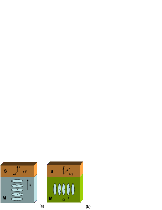
Figure 1: (Color online) The sketches of the spiral SSV in two configurations: spiral vector ${\bf Q}$ (a) orthogonal to the superconducting interface (opening of the LRTC channel), or (b) parallel to the superconducting interface.

Calculation method. For simplicity, we consider a S layer with a finite thickness $d_{s}$ covering a semi-infinite M layer with the vector $\bf{Q}$, along the $OZ$ direction, which may be parallel or orthogonal with respect to the interlayer interface (see Fig. 1). For the $T_{c}$ calculations, we assume the diffusive limit, because real superconducting nanostructures made by sputtering are usually dirty. In this case, the superconducting coherence lengths in the M and S layers are given by $\xi_{f,s}=\sqrt{D_{f,s}/2\pi T_{cb}}$, where $D_{f,s}$ is the corresponding diffusion coefficient and $T_{cb}$ is the critical temperature of the bulk superconductor. Close to $T_{c}$, superconducting correlations are weak, so that we can describe the underlying physics in the framework of the linearized Usadel equations.

The triplet proximity effect in the presence of a spiral or conical magnet has been intensively studied both theoretically in either the dirty Champel2005 ; VolkovAnishchanka ; Halasz2009 ; Halasz2011 or the clean Wu2012 ; USA2014 ; Halterman2016 regimes and experimentally RobinsonScience ; Sosnin2006 ; Zhu2013 ; Blamire2014b ; Blamire2015 ; Aarts2015 ; Chiodi2013 ; DiBernardo2015 ; Satchell2017 in complex multilayered magnetic structures designed for revealing LRTC. The theoretical work in Refs. VolkovAnishchanka ; Halasz2009 treated the critical current in S-M-S Josephson junctions with a conical vector orthogonal to the interface. Ref. Halasz2009, assumed the limit of a short spiral wavelength $\lambda\ll\xi_{f}$, which is suitable for Ho but not for MnSi. The case of a long wavelength was considered in Ref. VolkovAnishchanka, with a helicoidal magnet model, but the effect on $T_{c}$ was not investigated. The $T_{c}$ calculation in the parallel configuration (b) as depicted in Fig. 1 was published in Ref. Champel2005 , which only considered changes in $T_{c}$ with respect to the amplitude of ${\bf Q}$, not with respect to its direction (which is the topic of this paper).

The linearized Usadel equations for the singlet $f_{s}$ and triplet ${\bf f}_{t}=(f_{x},f_{y,}f_{z})$ spin components of the anomalous Green’s function, describing superconducting correlations, have the following form: Champel2005

$$\left(D_{f,s}\nabla^{2}-2\left|\omega\right|\right)f_{s} = -2\pi\Delta+2i\ \mathrm{sgn}(\omega){\bf h}\cdot{\bf f}_{t},$$ (1)

$$\left(D_{f,s}\nabla^{2}-2\left|\omega\right|\right){\bf f}_{t} = 2i\ \mathrm{sgn}(\omega){\bf h}f_{s}.$$

The singlet superconducting order parameter $\Delta$ is nonzero only in the S layer, while the exchange field ${\bf h}=h(\cos Qz,\sin Qz,0)$ is nonzero and aligned along the local magnetization in the M layer. The spiral vector ${\bf Q}$ is always taken parallel to $OZ$ axis. Since $h_{z}=0$, the third triplet component $f_{z}=0$. Using the unitary transformation $f_{\pm}=\left(\mp f_{x}+if_{y}\right)\exp(\pm iQz)$ and taking into account the symmetry of the Green’s functions with respect to the Matsubara frequency $\omega\equiv\omega_{n}=\pi T(2n+1)$ with $n$ an integer, we may rewrite Eqs. (1) for $\omega\geq 0$ as

$$\left(D_{f,s}\nabla^{2}-2\omega\right)f_{s}=-2\pi\Delta+i\ h\left(f_{-}-f_{+}\right),\hskip 42.67912pt$$ (2)

$$\left(D_{f,s}\nabla^{2}\mp 2iD_{f,s}Q\partial_{z}-D_{f,s}Q^{2}-2\omega\right)f_{\pm}=\mp 2i\ hf_{s}.$$

Eqs. (2) are supplemented by boundary conditions KL at $r=0$, where the coordinate $r=z$ or $r=y$ refers to the distance from the S/M interface depending on the chosen spiral configuration

$$\xi_{s}\partial_{r}f_{s,x,y}^{S}=\gamma\xi_{f}\partial_{r}f_{s,x,y},\,\,f_{s,x,y}^{S}=f_{s,x,y}-\gamma_{b}\xi_{f}\partial_{r}f_{s,x,y},$$ (3)

with the dimensionless interface parameters $\gamma_{b}=R_{b}A\sigma_{f}/\xi_{f}$ and $\gamma=(\sigma_{f}/\sigma_{s})(\xi_{s}/\xi_{f})$ ($R_{b}$ and $A$ are the resistance and the area of the S-M interface, respectively, and $\sigma_{f,s}$ is the conductivity of the M or S metal). Boundary conditions (3) relate the superconducting correlations coming from each side of the interface. The correlations in the S layer (located at $r<0$) are described by the functions $f_{s,x,y}^{S}$, while the functions $f_{s,x,y}$ contain the information about the structure of the M layer ($r>0$).

One obtains via some straightforward algebra (see supplementary material) a closed boundary value problem for the singlet component $f_{s}^{S}$ with the following boundary condition at the S/M interface: $\left.\xi_{s}\partial_{r}f_{s}^{S}\right|_{r=0}=-\left.Wf_{s}^{S}\right|_{r=0}$. The proximity effect in the M layer is entirely encapsulated in the real-valued quantity $W$. This key-quantity is the subject of the subsequent calculations considering two different spiral alignments in the M layer. The triplet solutions of Eqs. (2) in the S layer $f_{x,y}^{S}$ may be found in a simple exponential form with the wave vector $k_{s}=\sqrt{Q^{2}+2|\omega|/D_{s}}$. Eqs. (2) for the singlet component include the coordinate-dependent $\Delta$, which should be calculated self-consistently. The transition temperature of the structure, $T_{c}$, is computed numerically from

$$\ln\frac{T_{cb}}{T_{c}}=\pi T_{c}\sum_{\omega=-\infty}^{\infty}\left(\frac{1}{\left|\omega\right|}-\frac{f_{s}^{S}}{\pi\Delta}\right)$$ (4)

by using the method of fundamental solution Fominov2002 ; Champel2005 ; Lofwander07 .

Configuration (a): The spiral vector is orthogonal to the S layer. In this case, the problem becomes one-dimensional as in Ref. VolkovAnishchanka, with $r=z$ and $\nabla^{2}=\partial^{2}_{z}$. The M layer is infinite, so that the functions $f_{s,x,y}$ in the magnetic layer are sought under the form of decaying exponents $\exp(-kz)$ with $k$ a wave vector determined from the characteristic equation of the linear system (2)

$$\left[(k^{2}-k_{\omega}^{2}-Q^{2})^{2}+4Q^{2}k^{2}\right]\left(k^{2}-k_{\omega}^{2}\right)$$

$$+4k_{h}^{4}(k^{2}-k_{\omega}^{2}-Q^{2})=0,$$ (5)

where $k_{\omega}^{2}=2\omega/D_{f}$ and $k_{h}^{2}=h/D_{f}$. Provided that $k_{h}^{2}\gg Q^{2}>k_{\omega}^{2}$, Eq. (5) yields 3 complex-valued eigenvalues: two solutions $~{}k_{\pm}=\left(1\pm i\right)k_{h}$ of the order of $k_{h}$ describing short-range correlations and one real solution $k_{0}=\sqrt{k_{\omega}^{2}+Q^{2}}$ of the order of $Q$ characterizing long-range correlations. The reflected short- or long-range waves are neglected, so the M layer should be thicker than $max{[\lambda/\pi,2\xi_{f}]}$ to be considered as semi-infinite. Boundary conditions (3) together with triplet solutions of Eqs. (2) in the exponential form with the wave vectors $k_{s}$ in the S layer yield the quantity $W$ when the vector ${\bf Q}$ is orthogonal to the S layer:

$$W_{\perp}=\frac{\gamma\mathrm{Re}\left\{\xi_{f}k_{+}\left[(1+\xi_{c}k_{-})\left(1+\xi_{c}k_{0}\right)-(\xi_{c}Q)^{2}\right]\right\}}{\mathrm{Re}\{\left(1+\gamma_{b}\xi_{f}k_{+}\right)\left[(1+\xi_{c}k_{-})\left(1+\xi_{c}k_{0}\right)-(\xi_{c}Q)^{2}\right]\}},$$ (6)

with the length $\xi_{c}\equiv\xi_{f}\left[\gamma\coth(k_{s}d_{s})/k_{s}\xi_{s}+\gamma_{b}\right]$. The terms containing $Q$ and $k_{0}$ typically characterize the contribution of the long-range triplet correlations.

Configuration (b): The spiral vector is parallel to the S layer. We assume that the interface coincides with the $XOZ$ plane. Since the structure breaks translation invariance in the $r=y$ direction and the magnetic structure is nonuniform in the $z$ direction, the kinetic energy operator now reads $\nabla^{2}=\partial^{2}_{y}+\partial^{2}_{z}$. It has been shown in Ref. Champel2005, that $z$-independent correlations $f_{s,\pm}$ provide the lowest $T_{c}$ (i.e., they are the most favorable energetically), because they are the only solutions which realize a spatially homogeneous superconducting order parameter in the S layer at large distance from the S/M interface. In this case, we have the triplet vector ${\bf f}_{t}||{\bf h}$, meaning that only short-range triplet components are present.

More precisely, solutions of Eq. (2) in the M layer have again the form of decaying exponents with the wave vectors $k$ determined by a characteristic equation, with, however, an expresion now simpler than given by Eq. (5),

$$(k^{2}-k_{\omega}^{2}-Q^{2})^{2}(k^{2}-k_{\omega}^{2})+4k_{h}^{4}(k^{2}-k_{\omega}^{2}-Q^{2})=0.$$ (7)

This equation has an exact solution with two short-range eigenvalues $\tilde{k}_{\pm}=\sqrt{2k_{\omega}^{2}+Q^{2}/2\pm(i/2)\sqrt{16k_{h}^{4}-Q^{4}}}$ and a long-range one $k_{0}=\sqrt{k_{\omega}^{2}+Q^{2}}.$ Under the inequalities $k_{h}^{2}\gg Q^{2}$ and $k_{\omega}^{2}$, one gets $\tilde{k}_{\pm}\approx k_{\pm}$, so that respective eigenvectors coincide with those obtained for the case of the orthogonal spiral. Thus, under these conditions, the general form of the superconducting correlations in the M layer in the parallel configuration is identical to that in the orthogonal configuration. The major difference takes place only in the boundary conditions: since $\partial_{y}\exp(\pm iQz)=0$, the LRTC with the eigenvector $k_{0}$ now has no source neither in the S nor in the M layers, nor at the interface. Following the same steps as in the configuration (a), we get after straightforward algebra the quantity $W$ when ${\bf Q}$ is parallel to the S layer:

$$W_{\parallel}=\frac{\gamma\mathrm{Re}\left[\xi_{f}\tilde{k}_{+}\left(1+\xi_{c}\tilde{k}_{-}\right)\left(\sqrt{16k_{h}^{4}-Q^{4}}+iQ^{2}\right)\right]}{\mathrm{Re}\left[\left(1+\gamma_{b}\xi_{f}\tilde{k}_{+}\right)\left(1+\xi_{c}\tilde{k}_{-}\right)\left(\sqrt{16k_{h}^{4}-Q^{4}}+iQ^{2}\right)\right]}.$$ (8)

In contrast to $W_{\perp}$, we note that $W_{\parallel}$ does not contain $k_{0}$ characterizing the long-range triplet correlations.

Numerical results and discussion. For the calculations, we have assumed a S layer made of Nb. Bulk Nb has a critical temperature $T_{cb}=9.2$ K. Other data about Nb needed for the calculations are taken from the experimental work Flokstra2015 , where, for instance, $\xi_{s}=11$ nm. Ho magnets displaying conical spiral order have already been used in several hybrid structures RobinsonScience ; Sosnin2006 ; Blamire2015 in combination with Nb. The control of the superconducting state by a change of the magnetic state has even been obtained in recent experiments DiBernardo2015 ; Satchell2017 . However, the helimagnets Ho or Er used in these experiments have a strong in-plane magnetic anisotropy (with a spiral vector remaining orthogonal to the layer plane), so they do not appear as the best choice for the proposed SSV. Furthermore, an increase in the temperature of the sample above the Curie temperature (much higher than $T_{c}$) is needed in order to return to the initial helimagnetic state Satchell2017 , which makes this kind of switch difficult to use in low-temperature electronics.

In contrast, the transition-metal compounds of the MnSi family have a weak magnetic anisotropy (much smaller than the exchange energy $h$). They crystallize in a noncentrosymmetric cubic B20 structure, allowing a linear gradient invariant Bak1980 . This gives rise to a long-period spiral magnetic structure ($\lambda=18$ nm for MnSi). The existence of a domain structure with different spiral directions in neighboring domains was observed in such compounds Grigoriev2006b . Importantly, the spiral direction may be switched in not too large magnetic fields Grigoriev2006 . In MnSi, the spiral wave vector ${\bf Q}$ is aligned along [111] and equivalent directions of the cubic lattice. The angle between these directions is $\alpha=\arccos(1/3)=70.5^{\circ}.$ If one spiral axis is parallel to the S layer plane and another one is inclined by $\alpha$ with respect to this plane, then the period of the in-plane magnetic inhomogeneity is $\lambda/\cos\alpha=3\lambda\gg\xi_{s}$, which allows neglecting the in-plane inhomogeneity. In Eqs. (6) and (8), the value $Q$ changes to $Q\sin\alpha\approx 0.94Q$, and the behavior is practically the same as for $\alpha=90^{\circ}$. Considering transport properties Lee2007 ; Jonietz2010 , we used the following parameters for diffusive MnSi: $\xi_{f}=4.2$ nm and $\gamma=0.7$. The other estimations are $h\sim 100$ meV that is much less than the Fermi energy $\sim 1$ eV, and $Q=2\pi/\lambda\approx 0.35\,{\rm nm}^{-1}$. As a result, one gets $k_{h}\sim 0.7\,{\rm nm}^{-1}$ and $k_{\omega}\sim 0.14\,{\rm nm}^{-1}$. The inequalities $k_{h}>Q>k_{\omega}$ are fulfilled, thus justifying the approximations made in the derivation of quantity $W$.

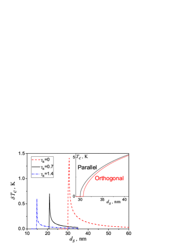
Figure 2: (Color online) Change in the superconducting critical temperature $\delta T_{c}$ at the crossover between the two spiral configurations shown in Fig. 1 as a function of the S layer thickness $d_{s}$ for different $\gamma_{b}$ values.

The numerical results for $T_{c}$ are displayed in Fig. 2. The magnetic switch from the parallel to the inclined configuration creates the condition for the LRTC appearance in the superconducting spin valve. As clearly seen in the inset of Fig. 2 showing an ideal situation for the SSV where the interlayer resistance $\gamma_{b}$ is neglected, the related drainage of Cooper pairs from the S layer effectively increases the proximity effect and suppresses $T_{c}$. The difference $\delta T_{c}$ between the two $T_{c}$ obtained in each magnetic configuration is shown in the main panel of Fig. 2 for different values of $\gamma_{B}$. It increases when the thickness of the S layer approaches the critical thickness corresponding to a total disappearance of superconductivity. Naturally, at this thickness, the superconducting film is most sensitive to the proximity effect. The two left curves account for a more realistic case with $\gamma_{b}=0.7$, calculated according to Eq. (A14) of Ref. PugachPRB2011, , and a twice larger $\gamma_{b}=1.4$, assuming an additional interface tunnel barrier. The experimental value of the coupling between Nb and a weak ferromagnet RyazanovPRL2006 was $\gamma_{b}=0.5$. As expected, the consequence of $\gamma_{b}$ is to weaken the superconducting proximity effect. The maximum value of $\delta T_{c}\sim 1$ K is obtained at the thickness where the S layer turns to the normal state in the orthogonal configuration. For realistic nonzero $\gamma_{b}$, the values of $\delta T_{c}$, which are between one- to a few hundred mK, may be still noticeable. This theoretical result indicates a spin-valve effect in the S-M bilayer at $\gamma_{b}=0$, of the same order of magnitude as predicted Fominov2010 in triplet SFF spin-valves in the same approximation footnote .

SSV structures are promising for application as elements of magnetic memory for low-temperature electronics, which has become recently a rapidly developing research direction Baek2014 ; Birge2014 related to the urgent need for energy-efficient logic for supercomputers. Usage of only one S layer and a bulk M layer should significantly simplify the SSV production technology. Another crucial feature of the proposed SSV is as follows: The switch of a particular memory element in a random access memory (RAM) device is carried out by a net of two crossed arrays of control electrodes. When the recording signal is sent along two crossed lines, the memory element located at the intersection of these lines changes its state, while all other element states in the same row or in the same column (thus receiving only one half of the signal) as the selected element remain unperturbed. Thus, the control signal should be able to switch the element state, whereas the half-amplitude signal should not cause a switch. The existence of a potential barrier between the two equilibrium spiral alignments in the magnetic part of the SSV provides an intrinsic solution to this half-select problem Vernik2013 . In contrast, this property is not present in previously studied triplet SSVs based on the continuous rotation of magnetization of one the ferromagnetic layers.

In conclusion, we have proposed a superconducting spin valve, consisting of a thin superconducting layer covered by a bulk spiral ferromagnet with multiple equilibrium configurations, such as MnSi. Its principle of operation is based on the controlled manipulation of long-range spin-triplet superconducting correlation in the structure. Our numerical results indicate that the spin-valve effect in these structures may be noticeable. Such spin-valves are superior in various regards compared to previously studied spin-valve geometries.

See supplementary material for a detailed calculation of the closed boundary conditions for the singlet component of the anomalous Green’s function in the S layer.

This work benefited from the Visiting Scientist Program of the Centre de Physique Théorique de Grenoble-Alpes and from the Royal Society International Program (IE150246). Also, N.P. thanks the Project N T3-89 “Macroscopic quantum phenomena at low and ultralow temperatures” of the National Research University Higher School of Economics, Russia.

Supplementary Material: Calculation of the closed boundary conditions for the S layer

To obtain the quantity $W$ in the closed boundary conditions $\xi_{s}\partial_{r}\left.f_{s}^{S}\right|_{r=0}=-W\left.f_{s}^{S}\right|_{r=0}$, we should recalculate it from the solution of the boundary-value problem for the triplet components in the S and M materials. This quantity $W$ entirely describes the proximity effect of the M layer.

The $r$-dependence of the triplet components in the S layer should also obey to the boundary condition at the free S interface

$$\frac{\partial}{\partial r}f_{s,x,y}^{S}(-d_{s})=0.$$

The solution of the Usadel equations (2) satisfying the boundary condition (S1) may be written in the form:

$$f_{x}^{S}=C_{x}\frac{\cosh\left[k_{s}(r+d_{s})\right]}{\sinh\left[k_{s}d_{s}\right]},$$

$$if_{y}^{S}=C_{y}\frac{\cosh\left[k_{s}(r+d_{s})\right]}{\sinh\left[k_{s}d_{s}\right]},$$

where $k_{s}=\sqrt{Q^{2}+2|\omega|/D_{s}}$. The coefficients $C_{x}$ and $C_{y}$ are found from the boundary conditions (3).

In the case of the spiral vector orthogonal to the S layer $r=z$, the characteristic equation (5) yields 3 eigenvalues $k_{\pm,0}$. The corresponding eigenvectors are $(-1,-1,1),~{}(1,-1,1)$ for $k_{\pm}$, and $(0,1,1)$ for $k_{0}$. These results entirely coincide with those obtained in Ref. [36].

Therefore, considering the above inequalities, the solution of coupled Eqs. (2) reads in the M layer:

$$f_{s}(z)=-A_{1}\exp(-k_{+}z)+A_{2}\exp(-k_{-}z),$$

$$f_{\pm}(z)=\pm A_{1}\exp(-k_{+}z)\pm A_{2}\exp(-k_{-}z)+A_{0}\exp(-k_{0}z).$$

Using boundary conditions (3) and relations (S2)-(S4) for the triplet components, we then get a first set of 4 equations for the coefficients $A_{0,1,2}$ and $C_{x,y}$

$$\xi_{s}\frac{\partial}{\partial z}f_{x}^{S}=\gamma\xi_{f}\left[A_{1}k_{+}+A_{2}k_{-}-iQA_{0}\right],$$

$$\xi_{s}\frac{\partial}{\partial z}f_{y}^{S}=-\gamma\xi_{f}\left[A_{0}k_{0}+iQ\left(A_{1}+A_{2}\right)\right],$$

$$C_{x}\coth k_{s}d_{s}=-A_{1}-A_{2}-\gamma_{b}\xi_{f}\left(A_{1}k_{+}+A_{2}k_{-}-iQA_{0}\right),$$

$$C_{y}\coth k_{s}d_{s}=A_{0}+\gamma_{b}\xi_{f}\left[A_{0}k_{0}+iQ\left(A_{1}+A_{2}\right)\right].$$

By writing boundary conditions (3) for the singlet component, we obtain two additional equations

$$\xi_{s}\frac{\partial}{\partial z}f_{s}^{S} = \gamma\xi_{f}\left(A_{1}k_{+}-A_{2}k_{-}\right),$$

$$f_{s}^{S} = -A_{1}+A_{2}-\gamma_{b}\xi_{f}\left(A_{1}k_{+}-A_{2}k_{-}\right),$$

which, by eliminating the coefficients $A_{0,1,2}$ and $C_{x,y}$, yield the quantity $W$ in the orthogonal configuration [Eq. (6)] .

The calculation of the quantity $W$ [Eq. (8)] for the case where the spiral vector ${\bf Q}$ is parallel to the S layer is carried out in the same way.

References

- (1) M. Eschrig, Phys. Today 64, No. 1, 43 (2011).
- (2) J. Linder and J. W. A. Robinson, Nat. Phys. 11, 307 (2015).
- (3) M. Eschrig, Rep. Prog. Phys. 78, 104501 (2015).
- (4) D. S. Holmes, A. L. Ripple, and M. A. Manheimer, IEEE Trans. Appl. Supercond. 23, 1701610 (2013).
- (5) S. Oh, D. Youm, and M. R. Beasley, Appl. Phys. Lett. 71, 2376 (1997).
- (6) A. I. Buzdin, A. V. Vedyayev, and N. V. Ryzhanova, Europhys. Lett. 48, 686 (1999).
- (7) L. R. Tagirov, Phys. Rev. Lett. 83, 2058 (1999).
- (8) Ya. V. Fominov, A. A. Golubov, T. Y. Karminskaya, M. Yu. Kupriyanov, R. G. Deminov, and L. R. Tagirov, JETP Lett. 91, 308 (2010).
- (9) A. Singh, S. Voltan, K. Lahabi, and J. Aarts, Phys. Rev. X 5, 021019 (2015).
- (10) P. V. Leksin, A. A. Kamashev, N. N. Garif’yanov, I. A. Garifullin, Ya. V. Fominov, J. Schumann, C. Hess, V. Kataev, and B. Büchner, JETP Lett. 97, 478 (2013).
- (11) F. S. Bergeret, A. F. Volkov, and K. B. Efetov, Phys. Rev. B 64, 134506 (2001).
- (12) A. Kadigrobov, R. I. Shekhter, and M. Jonson, Europhys. Lett. 54, 394 (2001).
- (13) M. Eschrig, J. Kopu, J. C. Cuevas, and Gerd Schön, Phys. Rev. Lett. 90, 137003 (2003).
- (14) F. S. Bergeret, A. F. Volkov, and K. B. Efetov, Rev. Mod. Phys. 77, 1321 (2005).
- (15) R. S. Keizer, S. T. B. Goennenwein, T. M. Klapwijk, G. Miao, G. Xiao, and A. Gupta, Nature 439, 825 (2006).
- (16) T. S. Khaire, M.A Khasawneh, W. P. Pratt, and N. O. Birge, Phys. Rev. Lett. 104, 137002 (2010).
- (17) J. W. A. Robinson, J. D. S. Witt, and M. G. Blamire, Science 329, 59 (2010).
- (18) K. Westerholt, D. Sprungmann, H. Zabel, R. Brucas, B. Hjorvarsson, D. A. Tikhonov, and I. A. Garifullin, Phys. Rev. Lett. 95, 097003 (2005).
- (19) P. V. Leksin, N. N. Garif’yanov, I. A. Garifullin, Y. V. Fominov, J. Schumann, Y. Krupskaya, V. Kataev, O. G. Schmidt, and B. Büchner, Phys. Rev. Lett. 109, 057005 (2012).
- (20) V. I. Zdravkov, J. Kehrle, G. Obermeier, D. Lenk, H. -A. Krug von Nidda, C. Müller, M. Yu. Kupriyanov, A. S. Sidorenko, S. Horn, R. Tidecks et al., Phys. Rev. B 87, 144507 (2013).
- (21) A. Iovan, T. Golod, and V. M. Krasnov, Phys. Rev. B 90, 134514 (2014).
- (22) A. A. Jara, C. Safranski, I. N. Krivorotov, C.-T. Wu, A. N. Malmi-Kakkada, O. T. Valls, and K. Halterman, Phys. Rev. B 89, 184502 (2014).
- (23) X. L. Wang, A. Di Bernardo, N. Banerjee, A. Wells, F. S. Bergeret, M. G. Blamire, and J. W. A. Robinson, Phys. Rev. B 89, 140508 (2014).
- (24) N. Banerjee, C. B. Smiet, R. G. J. Smits, A. Ozaeta, F. S. Bergeret, M. G. Blamire, and J. W. A. Robinson, Nat. Commun. 5, 3048 (2014).
- (25) M. G. Flokstra, T. C. Cunningham, J. Kim, N. Satchell, G. Burnell, P. J. Curran, S. J. Bending, C. J. Kinane, J. F. K. Cooper, S. Langridge et al., Phys. Rev. B 91, 060501(R) (2015).
- (26) R. G. Deminov, L. R. Tagirov, R. R. Garifullin, T. Yu. Karminskaya, M. Yu. Kuprianov, Ya. V. Fominov, and A. A. Golubov, J. Magn. Magn. Mater. 373, 16 (2015).
- (27) P. V. Leksin, N. N. Garif’yanov, A. A. Kamashev, A. A. Validov, Ya. V. Fominov, J. Schumann, V. Kataev, J. Thomas, B. Büchner, and I. A. Garifullin, Phys. Rev. B 93, 100502 (2016).
- (28) P. V. Leksin, A. A. Kamashev, J. Schumann, V. E. Kataev, J. Thomas, B. Büchner, and I. A. Garifullin, Nano Research 9, 1005 (2016).
- (29) Y. Ishikawa, G. Shirane, J. A. Tarvin, and M. Kohgi, Phys. Rev. B 16, 4956 (1977).
- (30) C. Pfleiderer, S. R. Julian, and G. G. Lonzarich, Nature 414, 427 (2001).
- (31) M. Uchida, Y. Onose, Y. Matsui, and Y. Tokura, Science 311, 359 (2006).
- (32) S. Mühlbauer, B. Binz, F. Jonietz, C. Pfleiderer, A. Rosch, A. Neubauer, R. Georgii, and P. Böni, Science 323, 915 (2009).
- (33) A. Fert, V. Cros, and J. Sampaio, Nature Nanotech. 8, 152 (2013).
- (34) T. Champel and M. Eschrig, Phys. Rev. B 71, 220506(R) (2005); ibid. 72, 054523 (2005).
- (35) T. Champel, T. Löfwander, and M. Eschrig, Phys. Rev. Lett. 100, 077003 (2008).
- (36) A. F. Volkov, A. Anishchanka, and K. B. Efetov, Phys. Rev. B 73, 104412 (2006).
- (37) G. B. Halász, J. W. A. Robinson, J. F. Annett, and M. G. Blamire, Phys. Rev. B 79, 224505 (2009).
- (38) G. B. Halász, M. G. Blamire, and J. W. A. Robinson, Phys. Rev. B 84, 024517 (2011).
- (39) C.-T. Wu, O. T. Valls, and K. Halterman, Phys. Rev. B 86, 184517 (2012).
- (40) K. Halterman and M. Alidoust, Phys. Rev. B 94, 064503 (2016).
- (41) I. Sosnin, H. Cho, V. T. Petrashov, and A. F. Volkov, Phys. Rev. Lett. 96, 157002 (2006).
- (42) L. Y. Zhu, Y. Liu, F. S. Bergeret, J. E. Pearson, S. G. E. te Velthuis, S. D. Bader, and J. S. Jiang, Phys. Rev. Lett. 110, 177001 (2013).
- (43) F. Chiodi, J. D. S. Witt, R. G. J. Smits, L. Qu, G. B. Halász, C.-T. Wu, O. T. Valls, K. Halterman, J. W. A. Robinson, and M. G. Blamire, Europhys. Lett. 101, 37002 (2013).
- (44) Y. Gu, G. B. Halász, J. W. A. Robinson, and M. G. Blamire, Phys. Rev. Lett. 115, 067201 (2015).
- (45) A. Di Bernardo, S. Diesch, Y. Gu, J. Linder, G. Divitini, C. Ducati, E. Scheer, M.G. Blamire, and J.W.A. Robinson, Nat. Commun. 6, 8053 (2015).
- (46) N. Satchell, J. D. S. Witt, M. G. Flokstra, S. L. Lee, J. F. K. Cooper, C. J. Kinane, S. Langridge, and G. Burnell, Phys. Rev. Applied 7, 044031 (2017).
- (47) M. Yu. Kuprianov and V. F. Lukichev, Zh. Eksp. Teor. Fiz. 94, 139 (1988) [Sov. Phys. JETP 67, 1163 (1988)].
- (48) Ya. V. Fominov, N. M. Chtchelkatchev, and A. A. Golubov, Phys. Rev. B 66, 014507 (2002).
- (49) T. Löfwander, T. Champel, and M. Eschrig, Phys. Rev. B 75, 014512 (2007).
- (50) P. Bak and M. H. Jensen, J. Phys. C: Solid State Phys. 13, L881 (1980).
- (51) S. V. Grigoriev, S. V. Maleyev, A. I. Okorokov, Yu. O. Chetverikov, P. Böni, R. Georgii, D. Lamago, H. Eckerlebe, and K. Pranzas, Phys. Rev. B 74, 214414 (2006).
- (52) S. V. Grigoriev, S. V. Maleyev, A. I. Okorokov, Yu. O. Chetverikov, and H. Eckerlebe, Phys. Rev. B 73, 224440 (2006).
- (53) M. Lee, Y. Onose, Y. Tokura, and N. P. Ong, Phys. Rev. B 75, 172403 (2007).
- (54) F. Jonietz, S. Mühlbauer, C. Pfleiderer, A. Neubauer, W. Münzer, A. Bauer, T. Adams, R. Georgii, P. Böni, R. A. Duine et al., Science 330, 1648 (2010).
- (55) N. G. Pugach, M. Yu. Kupriyanov, E. Goldobin, R. Kleiner, and D. Koelle, Phys. Rev. B 84, 144513 (2011).
- (56) V. A. Oboznov, V. V. Bol’ginov, A. K. Feofanov, V. V. Ryazanov, and A. I. Buzdin, Phys. Rev. Lett. 96, 197003 (2006).
- (57) B. Baek, W. H. Rippard, S. P. Benz, S. E. Russek, and P. D. Dresselhaus, Nat. Commun. 5, 3888 (2014).
- (58) In experiments such a sizable effect is usually considered as “giant” Aarts2015 ; Blamire2014 , but it is achieved only by using specific half-metallic ferromagnetic materials. In traditional metallic multilayered structures Westerholt2005 ; Leksin2012 ; Zdravkov2013 ; Krasnov2014 ; Blamire2014 ; Blamire2014b ; USA2014 ; Flokstra2015 ; TagirovKupr2015 ; Garifullin2016 ; Garifullin2016b the finite resistance of multiple interfaces suppresses the SSV effect. We may expect that the proposed SSV having only one interface does not suffer from this drawback.
- (59) B. M. Niedzielski, S. G. Diesch, E. C. Gingrich, Y. Wang, R. Loloee, W. P. Pratt, and N. O. Birge, IEEE Trans. Appl. Sup. 24 (4), 1800307 (2014).
- (60) I. V. Vernik, V. V. Bol’ginov, S. V. Bakurskiy, A. A. Golubov, M. Yu. Kupriyanov, V. V. Ryazanov, and O. A. Mukhanov, IEEE Trans. Appl. Supercond. 23, 1701208 (2013).