Two types of quasiperiodic partial synchrony in oscillator ensembles

Abstract

We analyze quasiperiodic partially synchronous states in an ensemble of Stuart-Landau oscillators with global nonlinear coupling. We reveal two types of such dynamics: in the first case the time-averaged frequencies of oscillators and of the mean field differ, while in the second case they are equal, but the motion of oscillators is additionally modulated. We describe transitions from the synchronous state to both types of quasiperiodic dynamics, and a transition between two different quasiperiodic states. We present an example of a bifurcation diagram, where we show the borderlines for all these transitions, as well as domain of bistability.

I Introduction

An ensemble of globally coupled limit-cycle oscillators is a widely used model for many natural systems Winfree (1967); *Winfree-80; Kuramoto (1984); Strogatz (2000); *Strogatz-03; Pikovsky et al. (2001a); Golomb et al. (2001); *Ott-book-02; *Manrubia-Mikhailov-Zanette-04; *Acebron-etal-05; *Breakspear-Heitmann-Daffertshofer-10. The main, well-understood, effect in this setup is emergence of a collective mode (mean field) via synchronization of ensemble elements Kuramoto (1975); *Sakaguchi-Kuramoto-86; Kuramoto (1984). Typical synchronization scenario is as follows. If a homogeneous coupling between generally non-identical ensemble units is attractive and quantified by parameter $\varepsilon>0$, then, typically, with the increase of $\varepsilon$ beyond some critical value, a number of oscillators adjust their (initially different) frequencies and form a synchronous group. The units in this group have coherent, though slightly different, phases and, as a result, produce a non-zero mean field. With the further increase of $\varepsilon$, more and more oscillators join the synchronous group and the mean field amplitude grows. The situation becomes almost trivial if the oscillators in the ensemble are identical: then full synchrony appears already for an arbitrarily small attractive coupling.

The described synchronization scenario assumes that the interaction remains attractive for all values of $\varepsilon$ and for all amplitudes of the collective mode. This is, however, not a general case: one can expect that weak and strong forcing on an oscillator may have different properties. In this paper we are interested exactly in the situations when the increase of the bifurcation parameter $\varepsilon$ results in a change of the interaction type from an attractive to a repulsive one, yielding complex regimes already for the simplest setups with identical units. In particular, our goal is to analyze the quasiperiodic partially synchronous (QPS) regimes that appear via a synchrony-breaking transition and are characterized by scattered or clustered oscillator states and yet non-vanishing collective mode; the most important feature is the quasiperiodic dynamics of oscillators. We describe two types of such solutions. In one case, which we denote as QPS-I, the time averaged frequencies of individual oscillators and of the mean field are different. In the second case, labeled as QPS-II, the averaged frequencies coincide, but the motion of oscillators is additionally modulated. We demonstrate that these regimes between full synchrony and complete asynchrony appear in an ensemble of Stuart-Landau (SL) oscillators with global nonlinear coupling. For this model, we analytically find the conditions for two bifurcations resulting in emergence of two types of QPS dynamics. Furthermore, we reveal transitions between the QPS-I and the QPS-II dynamics, as well as parameter domains where full synchrony coexists with the QPS states.

The paper is organized as follows. First we introduce our basic model in Section II. Then, in Section III we discuss the weak-coupling limit and properties of partial synchrony in the phase approximation. Next, in Section IV we analyze stability of the synchronous and of the asynchronous state for arbitrary coupling, and present the diagram of different states. Section V presents the results of numerical analysis. We discuss and summarize our results in Section VI.

II Stuart-Landau oscillators with global nonlinear coupling

Our basic model is a system of $N$ identical Stuart-Landau oscillators with global nonlinear coupling (cf. Pikovsky and Rosenblum (2009); Popovych et al. (2005); Schmidt et al. (2014); *PhysRevLett.114.034101):

$$\dot{a}_{k}=(1+\mathrm{i}\omega_{0}) a_{k}-(1+\mathrm{i}\alpha)|a_{k}|^{2}a_{k}$$

$$+(\varepsilon_{1}+\mathrm{i}\varepsilon_{2})A-(\eta_{1}+\mathrm{i}\eta_{2})|A|^{2}A\;,$$ (1)

where

$$A=\rho\mathrm{e}^{\mathrm{i}\Theta}=N^{-1}\sum_{k=1}^{N}a_{k}\;$$ (2)

is the complex mean field. Here $\omega_{0}$ is the frequency of small oscillations (it does not play any role since it can be eliminated by a transformation to a rotating reference frame) and $\alpha$ describes non-isochronicity of uncoupled oscillators. The coupling is quantified by four parameters: parameters $\varepsilon_{1,2}$ describe linear coupling term $\sim A$, while parameters $\eta_{1,2}$ describe nonlinear coupling $\sim|A|^{2}A$. Notice that the case of purely linear coupling was extensively studied by Hakim and Rappel Hakim and Rappel (1992) and by Nakagawa and Kuramoto Nakagawa and Kuramoto (1993); *Nakagawa-Kuramoto-94, see also Matthews et al. (1991); *PhysRevLett.93.104101; *PhysRevLett.96.054101. We come back to this case in the discussion section below.

In the synchronous regime $a_{1}=\ldots=a_{N}=r\mathrm{e}^{\mathrm{i}\varphi}=A$ and the stationary (uniformly rotating with frequency $\Omega$) solution of Eqs. (1) can be easily found:

$$r^{2}=\frac{1+\varepsilon_{1}}{1+\eta_{1}}\;,\qquad\Omega=\dot{\varphi}=\omega_{0}+\varepsilon_{2}-\frac{(\alpha+\eta_{2})(1+\varepsilon_{1})}{1+\eta_{1}}\;.$$ (3)

In the fully asynchronous regime the mean field $A$ vanishes. This state is microscopically degenerate, as there is just one condition on the distribution of $N$ phases. Stability of the asynchronous and synchronous states is studied in the next sections.

Before proceeding to a more general analysis, we mention one intermediate dynamical state which appears for a special set of parameters. Indeed, if the ratio $\frac{\varepsilon_{1}+\mathrm{i}\varepsilon_{2}}{\eta_{1}+\mathrm{i}\eta_{2}}$ is real, then for $|A|^{2}=\frac{\varepsilon_{1}+\mathrm{i}\varepsilon_{2}}{\eta_{1}+\mathrm{i}\eta_{2}}$ the coupling vanishes. In this regime, called “bunch state” in Pikovsky and Rosenblum (2009), the oscillators are partially synchronized, but the dynamics is purely periodic as all units have the same frequency $\omega_{0}-\alpha$.

III Weak coupling limit, phase approximation, and partial synchrony

III.1 Weak coupling limit

Close to the asynchronous regime, where the amplitude $A$ is small, the coupling between the oscillators is weak. This also holds for a non-small amplitude $A$, if coupling parameters are small $\varepsilon_{1,2}\ll 1$, $\eta_{1,2}\ll 1$. For such a weak coupling, the amplitudes $|a_{k}|$ are only slightly perturbed: $|a_{k}|\approx 1$. Then $a_{k}\approx\mathrm{e}^{\mathrm{i}\varphi_{k}}$ and the mean field $A$ is simply the Kuramoto order parameter $R\exp[\mathrm{i}\Theta]=N^{-1}\sum_{j}\exp[\mathrm{i}\varphi_{j}]$, $0\leqslant R\leqslant 1$. Using the standard approach Kuramoto (1984); Pikovsky et al. (2001a), Eq. (1) can be reduced to the phase dynamics:

$$\dot{\varphi}_{k}=\overline{\omega}+{\cal E}(R;\varepsilon_{1,2},\eta_{1,2})R\sin\left[\Theta-\varphi_{k}+\beta(R;\varepsilon_{1,2},\eta_{1,2})\right]\;,$$ (4)

where $\overline{\omega}=\omega_{0}-\alpha$, while the amplitude ${\cal E}\geqslant 0$ and the phase shift $\beta$ in the coupling are determined from

$${\cal E}\sin\beta =\alpha(R^{2}\eta_{1}-\varepsilon_{1})+\varepsilon_{2}-R^{2}\eta_{2}\;,$$ (5)

$${\cal E}\cos\beta =\varepsilon_{1}-R^{2}\eta_{1}-\alpha(R^{2}\eta_{2}-\varepsilon_{2})\;.$$

Equation (4) can be considered as a nonlinear generalization of the popular Kuramoto-Sakaguchi model Kuramoto (1975); *Sakaguchi-Kuramoto-86. Indeed, for the linear coupling $\eta_{1}=\eta_{2}=0$ we obtain exactly the Kuramoto-Sakaguchi model

$$\dot{\varphi}_{k}=\overline{\omega}+\varepsilon R\sin(\Theta-\varphi_{k}+\beta)\;,$$ (6)

where

$$\varepsilon^{2}=(\alpha\varepsilon_{1}-\varepsilon_{2})^{2}+(\alpha\varepsilon_{2}+\varepsilon_{1})^{2}\;,\;\beta=\text{Arg}(\varepsilon_{1}+\alpha\varepsilon_{2}+\mathrm{i}(\varepsilon_{2}-\alpha\varepsilon_{1}))\;.$$

Generally, if both linear and nonlinear couplings are present, instead of two constants $\varepsilon$ and $\beta$ we have two functions ${\cal E}(R;\varepsilon_{1,2},\eta_{1,2}),\;\beta(R;\varepsilon_{1,2},\eta_{1,2})$; this model has been suggested and studied in Rosenblum and Pikovsky (2007); Pikovsky and Rosenblum (2009). Notice that this phase model also appears as an approximation of the system of SL oscillators, coupled through a common nonlinear load Pikovsky and Rosenblum (2009). A very important property of the model (4) is its partial integrability: according to the Watanabe-Strogatz theory Watanabe and Strogatz (1993); *Watanabe-Strogatz-94; *Pikovsky-Rosenblum-11, dynamics of (4) is described by three global variables and $N-3$ constants of motion; this description is valid for any $N>3$, including the thermodynamic limit $N\to\infty$,

It is easy to see that synchronous solution of the model (4) is stable if
${\cal E}(1;\varepsilon_{1,2},\eta_{1,2})\cos\left[\beta(1;\varepsilon_{1,2},\eta_{1,2})\right]<0$. To determine stability of the asynchronous state, we have to consider effect of a small perturbation, i.e. effect of the mean field with $R\ll 1$. This means that we can neglect the terms $R^{2}\eta_{1,2}$ in (5) and the model reduces to the Kuramoto-Sakaguchi system (6). So, only the linear part of the coupling contributes to the instability of the asynchronous state. The asynchronous state will be unstable if the coupling is attractive, i.e. if $\cos\beta>0$. This condition yields instability provided $\varepsilon_{1}+\alpha\varepsilon_{2}>0$, and stability otherwise.

III.2 Partial synchrony and quasiperiodicity within phase approximation

Here we discuss partial synchrony in the framework of the phase approximation (4). A detailed analysis of this model has been presented in Rosenblum and Pikovsky (2007); Pikovsky and Rosenblum (2009), so we just reproduce the basic ideas for consistency.

Consider first the pure Kuramoto-Sakaguchi case (6). As is well-known, the synchronous state, $R=1$, is stable, if $|\beta|<\pi/2$, and unstable, if $\pi/2<\beta<3\pi/2$ (we remind that $\varepsilon>0$). For the asynchronous (splay) state, $R=0$, the stability conditions are reversed. Hence, there occurs either full synchrony or full asynchrony. Notice that existence of other attractive states with $0<R<1$ or of many-cluster solutions with $R=0$ is excluded by the Watanabe-Strogatz theory Watanabe and Strogatz (1993); *Watanabe-Strogatz-94; *Pikovsky-Rosenblum-11.

Complementarity of stability domains for synchronous and asynchronous solutions is a specific property of the Kuramoto-Sakaguchi model. For general globally coupled systems the situation can be different. So, we can expect overlap of stability domains for some parameter region; then, in this region, the system is at least bi-stable. Another possible case, of our interest here, is when both fully synchronous and fully asynchronous solutions are unstable. Then, for the corresponding parameters the system is enforced to settle at some non-trivial state between synchrony and asynchrony. An example is given by Eq. (4), where $\beta(R;\varepsilon_{1,2},\eta_{1,2})$ depends on the order parameter $R$. Stability of the asynchronous state is determined solely by $\beta(0,\varepsilon_{1,2},\eta_{1,2})$, while for the state of full synchrony, $R=1$, the value $\beta(1,\varepsilon_{1,2},\eta_{1,2})$ is relevant. If $\cos\beta(0,\varepsilon_{1,2},\eta_{1,2})>0$ and $\cos\beta(1,\varepsilon_{1,2},\eta_{1,2})<0$, both fully synchronous and asynchronous states are unstable (the border between stability and instability domains for the synchronous state is determined from the condition $\cos\beta(1,\varepsilon_{1,2},\eta_{1,2})=0$). It means, that an intermediate, partially synchronous state with $0<R<1$ is established. The order parameter in this state is given by the condition $\cos\beta(R,\varepsilon_{1,2},\eta_{1,2})=0$.

Next, we stress that system (4), like the Kuramoto-Sakaguchi model, is fully described by the Watanabe-Strogatz theory Watanabe and Strogatz (1993); *Watanabe-Strogatz-94; *Pikovsky-Rosenblum-11 which excludes the states with more than one synchronous cluster for general non-identical initial conditions. Hence, at partial synchrony, all phases shall be scattered and non-uniformly distributed on the unit circle. As it follows from Eq. (4), this scattering results in different instantaneous frequencies of all units. Furthermore, it results in the most peculiar feature of this state, namely in a difference of the time-average frequencies of the units and of the frequency of the mean field. Let us denote these frequencies as $\Omega$ and $\nu$, respectively. (Notice that since oscillators are identical, all $\Omega_{k}=\Omega$). In our previous publications Rosenblum and Pikovsky (2007); Pikovsky and Rosenblum (2009) we called such states with $0<R<1$ and $\Omega\neq\nu$ self-organized quasiperiodic (SOQ) solutions.

Qualitatively the property $\nu\neq\Omega=\langle\dot{\varphi}\rangle$ can be shown by contradiction. Suppose first the contrary, $\nu=\Omega$, and consider the motion in the frame, rotating with the mean field frequency $\nu$. Then, according to Eq. (4), the points, representing some oscillators move forwards and some of them move backwards with respect to the mean field. Hence, there are two values of $\varphi$ where the velocity in this frame changes its sign, and one of these values corresponds to stable state and another corresponds to an unstable one. So, the oscillators having these phase values are in rest. Other oscillators move towards the stable state and therefore merge into a cluster. Since clusters in this setup are not possible, the assumption $\nu=\Omega$ cannot be true. Hence, either all oscillators move faster than the mean field or all of them move slower, i.e. $\Omega\neq\nu$. A detailed quantitative analysis of system (4) can be found in Rosenblum and Pikovsky (2007); Pikovsky and Rosenblum (2009).

It is important to notice that the phase model (4) is only an approximation of the full system of Eqs. (1) for the case when the amplitude dynamics is enslaved. In this situation the amplitude perturbations decay rapidly, and instability of the fully synchronous state occurs due to one real eigenvalue, corresponding to the phase (as described in the next section). Thus, for weak coupling we can expect that the above described SOQ dynamics appears close to instability of the synchronous state of the full system, when one real multiplier becomes larger than unity. Here we denote such dynamics as QPS-I, to be distinguished from another quasiperiodic state, discussed below. However, the correspondence between QPS-I and SOQ is not exact, as due to corrections to the first-order model (4), some fine features may become different. For example, while in model (4) several clusters are not possible due to the Watanabe-Strogatz theory, already small perturbations to the model generally destroy this property and enable clustering.

IV Beyond the phase approximation

We analyze stability of the fully synchronous state Eq. (3) with respect to the evaporation of individual oscillators from the synchronous cluster. In fact, one can always consider purely transversal evaporation modes such that the mean field $A$ remains unchanged. Substituting $a_{k}=b_{k}e^{i\Omega t}$, we make transformation to the coordinate frame, rotating with the frequency $\Omega$, where $\Omega$ is given by Eq. (3). We obtain

$$\dot{b}_{k}=(1+\mathrm{i}\omega) b_{k}-(1+\mathrm{i}\alpha)|b_{k}|^{2}b_{k}$$

$$+(\varepsilon_{1}+\mathrm{i}\varepsilon_{2})B-(\eta_{1}+\mathrm{i}\eta_{2})|B|^{2}B\;,$$ (7)

where $\omega=\omega_{0}-\Omega$ and $B=N^{-1}\sum_{j}^{N}b_{j}$. In the new frame, synchronous motion corresponds to a resting point; we choose the coordinate system so that $b_{k}=B=r$. Linearizing the equation around this point while keeping $B=\mbox{const}$, we obtain after straightforward manipulations the eigenvalues

$$\lambda_{1,2}=(1-2r^{2})\pm\sqrt{(1-3\alpha^{2})r^{4}+4\omega\alpha r^{2}-\omega^{2}}\;,$$ (8)

related to evaporation multipliers as $|\mu|=\mathrm{e}^{\lambda T}$, where $T=2\pi/\Omega$ is the oscillation period Kaneko (1994); *Pikovsky-Popovych-Maistrenko-01; Rosenblum and Pikovsky (2007).

If both eigenvalues (8) are negative, the fully synchronous cluster is stable. The instability occurs when either one real eigenvalue becomes positive, or a pair of complex eigenvalues crosses the imaginary axis. The situation when one real eigenvalue $\lambda_{1}$ changes from negative to positive value is exactly the transition described in section III.2 above. One can check that the condition $\lambda_{1}=0$ in (8) in the limit of small coupling terms $\varepsilon_{1,2},\eta_{1,2}$ is exactly the condition $\cos\beta(1,\varepsilon_{1,2},\eta_{1,2})=0$ where $\beta$ is defined according to (5).

The comprehensive analysis of Eqs. (7,8) is hardly feasible due to a large number of parameters. Therefore, we consider here below only a special case of isochronous oscillators, $\alpha=0$, which demonstrates both types of synchrony-breaking transition, of our interest in this study. Additionally, we fix $\eta_{2}=0$, i.e. take purely dissipative nonlinear coupling. Furthermore, we consider $\varepsilon_{1,2}\geqslant 0$. Then, with account of Eq. (3), we find $\omega=\omega_{0}-\Omega=-\varepsilon_{2}$, what yields

$$\lambda_{1,2}=(1-2r^{2})\pm\sqrt{r^{4}-\varepsilon_{2}^{2}}\;.$$ (9)

Case of real eigenvalues.

The condition for the eigenvalues to be real is $r^{2}\geqslant\varepsilon_{2}$. The bifurcation takes place when $\lambda_{1}$ becomes zero, what yields $r^{2}=\frac{1}{3}\left(2\pm\sqrt{1-3\varepsilon_{2}^{2}}\right)\geqslant\varepsilon_{2}$. Hence, we have $\varepsilon_{2}\leqslant 1/\sqrt{3}\approx 0.577$ and the critical line is found from the equation

$$2\pm\sqrt{1-3\varepsilon_{2}^{2}}=3\frac{1+\varepsilon_{1}}{1+\eta_{1}}\;.$$ (10)

Bunch states.

Consider the case $\varepsilon_{2}=0$. The eigenvalues are $\lambda_{1}=1-r^{2}$, $\lambda_{2}=1-3r^{2}$. Hence, synchrony becomes unstable for $r<1$, i.e. for $\eta_{1}>\varepsilon_{1}$. Obviously, a neutrally stable state, $r=1$, $\Omega=\omega_{0}$, and $\rho=R=\sqrt{\varepsilon_{1}/\eta_{1}}$ is a solution of Eq. (1). The case corresponds to the bunch state, cf. also Popovych et al. (2005).

Case of complex eigenvalues.

The condition for the eigenvalues to be complex is $r^{2}<\varepsilon_{2}$ and the condition for the real part to be zero is $r^{2}=\frac{1+\varepsilon_{1}}{1+\eta_{1}}=\frac{1}{2}$. Hence, the critical line is determined by $\eta_{1}=1+2\varepsilon_{1}$ and $\varepsilon_{2}>0.5$. For $\varepsilon_{2}=0.5$ and $\eta_{1}=1+2\varepsilon_{1}$ we have the “Takens-Bogdanov point” $\lambda_{1,2}=0$.

Stability of the asynchronous state.

This is accomplished as described in section III.1. For the chosen parameters we obtain from (5) ${\cal E}^{2}=\varepsilon_{1}^{2}+\varepsilon_{2}^{2}$ and $\beta=\arctan{(\varepsilon_{2}/\varepsilon_{1})}$. Since $\varepsilon_{1,2}>0$, the asynchronous state is always unstable.

We emphasize that although synchrony breaking is quantified by only two eigenvalues (8), the transition cannot be described as a low-dimensional bifurcation, because all oscillator leave the synchronous cluster simultaneously, what means that in the original $N$-dimensional phase space there is $N-1$-fold degeneracy of eigenvalues (8).

For an example of the bifurcation diagram we fix $\varepsilon_{1}=3$; thus, our bifurcation parameters are $\varepsilon_{2}$ and $\eta_{1}$. The results are shown in Fig. 1. The blue solid line corresponds to Eq. (10); here the largest real eigenvalue turns zero. The red bold line $\eta_{1}=7$, $\varepsilon_{2}>0.5$ shows where the Hopf-like bifurcation (complex eigenvalues) takes place. Below the blue solid line and to the right of the red bold one the full synchrony is unstable and partially synchronous dynamics sets in.

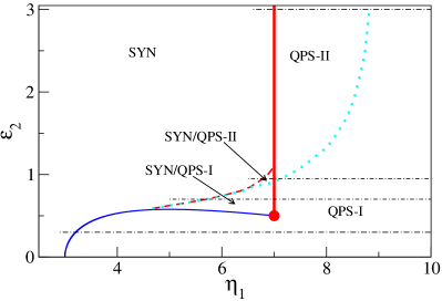
Figure 1: (Color online) Bifurcation diagram for $\varepsilon_{1}=3$. Blue solid line: here the largest real eigenvalue equals zero; red bold line: here real parts of complex roots are equal to zero. Red filled circle marks the Takens-Bogdanov point. Theoretical analysis is complemented by the numerical study, which reveals 5 domains: stable full synchrony (SYN), quasiperiodic partial synchrony (QPS-I and QPS-II), and two domains where bistability between synchrony and partial synchrony is observed (SYN/QPS-I and SYN/QPS-II). Red dashed and cyan dotted curves are obtained numerically; they denote emergence of the amplitude modulation and of the frequency difference, respectively, see text for details. The line $\varepsilon_{2}=0$, $\eta_{1}>3$ corresponds to the partially synchronous but not quasiperiodic bunch states. Four horizontal black dashed-dotted lines show the cuts of the diagram illustrated in Figs. 2,4,7,8 and in the text.

Next, we complement the diagram by the results of direct numerical simulation.

V Numerical exploration

All computations have been performed for $\omega_{0}=5$ and $N=501$. For several points in the diagram we checked that increasing of the ensemble size up to several thousands does not influence the results. We analyze the bifurcation diagram in Fig. 1, by describing transitions at several fixed values of $\varepsilon_{2}$ (marked with dashed-dotted lines) while parameter $\eta_{1}$ increases.

For $\varepsilon_{2}=0,\eta_{1}>3$, the solution is a partially synchronous bunch state (not shown). For small positive $\varepsilon_{2}$ (we have taken $\varepsilon_{2}=0.3$ for illustration), the dynamics beyond synchrony-breaking is quasiperiodic, as is shown in Fig. 2,3 and corresponds to regime QPS-I as described in section III.2. Beyond the bifurcation, the frequency difference $\nu-\Omega$ (we remind that $\Omega$ and $\nu$ are frequencies of an oscillator and of the mean field, respectively) smoothly grows, as well as the amplitude modulation of oscillators (this can be also appreciated from the phase portraits in Fig. 3). It can be also recognized, that the distribution of the points in a snapshot becomes more uniform with increase of $\eta_{1}$, what corresponds to decrease of the mean field amplitude. Notice that variations of the mean field frequency and of the amplitude are small, so that the mean field can be considered as harmonic.

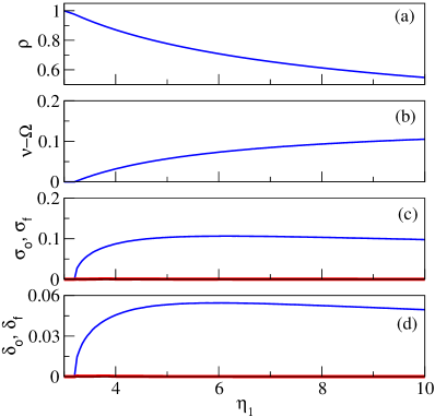
Figure 2: (Color online) Transition from synchrony to quasiperiodic partial synchrony of type I for small $\varepsilon_{2}=0.3$. (a) Mean field amplitude $\rho$. (b) Frequency difference is the essential feature of the QPS-I dynamics. Here we see that the mean field is faster than the oscillators, and that the frequency difference $\nu-\Omega$ smoothly grows beyond the transition point. (c) Frequency modulation of the oscillators and of the mean field is quantified by the standard deviations of their instantaneous frequencies, denoted as $\sigma_{o}$ and $\sigma_{f}$; these quantities are shown by blue solid and red bold curves, respectively. (d) Here blue solid and red bold curves show the standard deviations of oscillator and mean field amplitudes, denoted as $\delta_{o}$ and $\delta_{f}$, respectively.

Figure 3: (Color online) (a,b,c): Phase portraits, illustrating the synchrony-to-QPS-I transition at $\varepsilon_{2}=0.3$. Gray solid and blue bold curves show trajectories of an oscillator and of the mean field, respectively for $\eta_{1}=3.5$ (a), $\eta_{1}=7$ (b), and $\eta_{1}=10$ (c). Open circles (magenta) show a snapshot of the ensemble. (d,e,f): Probability distribution $\rho$ of instantaneous frequency of the oscillator, $\omega_{o}$ (bold black curve), and of the mean field, $\omega_{f}$ (red curve) for $\eta_{1}=3.5$, $\eta_{1}=7$, and $\eta_{1}=10$, respectively.

Next we consider large $\varepsilon_{2}=3$, see Fig. 4,5. In contrast to the case of small $\varepsilon_{2}$, we see that, with increase of $\eta_{1}$, the quasiperiodic motion initially appears due to the pure amplitude modulation (regime QPS-II). It means, that trajectory in the phase space lays on a torus that encircles the original limit cycle, and whose “thickness” grows smoothly with $\eta_{1}$. The ensemble elements split into several (quasi)clusters that rotate around the torus in such a way that $\nu=\Omega$. (We checked that for the parameters used for the phase portrait plots, the averaged frequencies and the amplitudes of all elements are the same up to numerical precision). Then, when $\eta_{1}$ attains some critical value, the frequency difference appears by a jump (dotted cyan curve in Fig. 1), and we observe a transition from QPS-II to QPS-I. Geometrically, this transition can be described as follows. With increase of $\eta_{1}$, the torus becomes more and more “thick” so that the minimal oscillation amplitude $|a|$ decreases and reaches zero at some value of $\eta_{1}$. From now on the rotation of the cluster encircles the origin on the $x,y$ plane, and, hence, the frequencies of an oscillator and of the mean field start to differ. With further increase of $\eta_{1}$, the minimal $|a|$ grows, but the trajectory continues to encircle the origin. Notice that at the transition from QPS-II to QPS-I, the frequency difference $\nu-\Omega$ emerges by a jump and then remains practically constant.

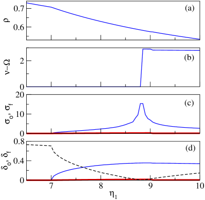
Figure 4: (Color online) Transition from synchrony to QPS-II and then to QPS-I, for $\varepsilon_{2}=3$. The shown quantities are same as in Fig. 2. In (d) we additionally show the minimal value of the oscillator amplitude $r$ (dashed curve). The first transition, synchrony to QPS-II, takes place at $\eta_{1}=7$, as predicted by the stability analysis. At this point the amplitude and frequency modulation of oscillators emerge smoothly, but the average frequencies are still equal, $\nu=\Omega$. At $\eta_{1}\approx 8.8$ the second transition takes place, here the frequency difference appears by jump.

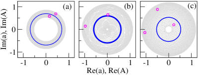
Figure 5: (Color online) Phase portraits, illustrating the transitions at $\varepsilon_{2}=3$, (the same curves as in Fig. 3). (a) QPS-II state, $\eta_{1}=7.1$. (b) Close to the transition from QPS-II to QPS-I, $\eta_{1}=8.5$. (c) QPS-I state at $\eta_{1}=10$.

In fact, the trajectories of (quasi)clusters cannot be easily recognized from the phase plots in Fig. 5. However, the dynamics becomes much more illustrative for slightly nonidentical units, as shown in Fig. 6. In this computation we take oscillator frequencies uniformly distributed in $\omega_{0}-\Delta,\omega_{0}+\Delta$, where $\Delta=0.001$. Noteworthy, for small $\varepsilon_{2}$, inhomogeneity does not affect the overall picture, but just slightly changes the threshold for synchrony breaking.

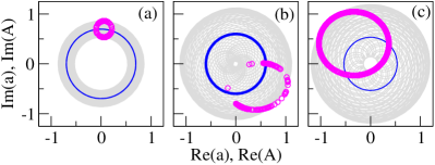
Figure 6: (Color online) Same as in Fig. 5, but for slightly non-identical oscillators. Now it is easy to see that the trajectory (represented by a sequence of oscillators’ states marked with circles) in (a) does not encircle the origin directly, but encircles the mean field, and therefore the frequency difference $\nu-\Omega=0$, this is the QPS-I state. The trajectory in (c) directly encircles the origin and therefore the frequencies differ, this is the QPS-II state.

Finally, we consider the intermediate values of $\varepsilon_{2}$. The essential novel feature here is bistability and hysteresis. It turns out that, with increase of $\eta_{1}$, a QPS state gains its stability while the synchronous state is still stable. Thus, partial and full synchrony coexist in this domain. (Practically, we performed simulations either starting from almost synchronous or from almost asynchronous initial conditions. Alternatively, to determine the stability domain of QPS we started from the partially synchronous state and decreased $\eta_{1}$.) Analysis shows that this domain contains sub-domains of QPS-I and QPS-II dynamics. For illustration, we consider synchrony-breaking transitions for two values of parameter $\varepsilon_{2}$, $\varepsilon_{2}=0.7$ and $\varepsilon_{2}=0.95$. In the former case, we observed a transition from synchrony to the QPS-I dynamics. In contrast to small $\varepsilon_{2}$ (cf. the picture for $\varepsilon_{2}=0.3$ in Fig. 2), here the frequency difference $\nu-\Omega$ and the amplitude modulation appear by a jump, see Fig. 7. In the latter case, $\varepsilon_{2}=0.95$, we first observed a transition from synchrony to QPS-II and then another transition to QPS-I. It means that in this case, with increase of $\eta_{1}$, first the amplitude modulation appears by a jump, and then the frequency difference appears at another critical value of the parameter.

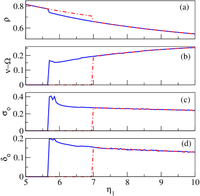
Figure 7: (Color online) Hysteresis at the transition from synchrony to QPS-I for $\varepsilon_{2}=0.7$. The shown quantities are mean field amplitude $\rho$ (a), frequency difference $\nu-\Omega$ (b), and standard deviations $\sigma_{o}$ (c) and $\delta_{o}$ (d) of the instantaneous frequency and of the amplitude of the oscillators. In each panel solid blue line shows the results obtained for nearly asynchronous initial conditions, while dashed-dotted red line corresponds to nearly synchronous initial conditions.

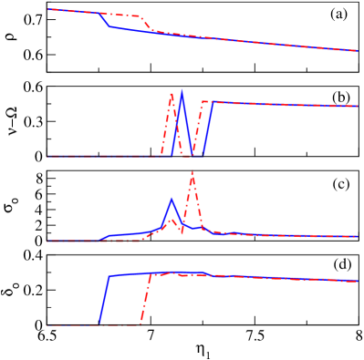
Figure 8: (Color online) Hysteresis at transitions between synchrony, QPS-I and QPS-II for $\varepsilon_{2}=0.95$. The shown quantities are the same as in Fig. 7.

To conclude this section, we mention that we cannot claim that the diagram in Fig. 1 yields a complete description of the dynamics, because it is not possible to check all possible initial conditions. For example, for some small parameter domain we have observed coexistence of both types of QPS dynamics. We cannot exclude other interesting dynamical regimes, but we believe that we have described the dominating solutions.

VI Discussion and conclusions

In this paper we analyzed two regimes of partially synchronous states in globally coupled identical oscillator populations. These regimes can be attributed to a type of bifurcation at the transition from full to partial synchrony: QPS-I corresponds to one real evaporation eigenvalue becoming positive, while regime QPS-II corresponds to two complex evaporation eigenvalues crossing real axis (in terms of multipliers, one real multiplier becomes larger than one or two complex multipliers become larger than one in absolute values). These transitions are roughly related to two typical bifurcations from a steady state to a periodic dynamics: SNIPER (saddle-node-infinite-period) and Hopf bifurcations. The main difference is that in ensembles of oscillators the transition is extremely high-dimensional (in fact, infinite-dimensional in the thermodynamic limit) so that usual low-dimensional bifurcation theory does not apply. In particular, while we can reliably describe some robust dynamical features like frequency difference between the mean field and the individual oscillators, other fine dynamical features such as appearance of clusters seem to be non-universal and strongly model-dependent.

For example, the simplest setup for the description of the regime QPS-I is the nonlinear extension of the Kuramoto-Sakaguchi model Eq. (4), but it does not allow for multiple clusters. For phase models with a general coupling function (not just one harmonics) of phase differences, called Daido models Daido (1993a); *Daido-93a; *Daido-95; *Daido-96, this does not hold. Therefore, for such models one can expect (i) scattered states, (ii) clustered states, (iii) and mixed states (scattered oscillators plus cluster(s)). These states may also be quasiperiodic. Certainly, the same can be said if one goes beyond the phase dynamics approximation and analyzes globally coupled multidimensional oscillators. To the type (iii) belong also chimera states (Kuramoto and Battogtokh, 2002; *Abrams-Strogatz-04; *PhysRevLett.100.044105; *Abrams-Mirollo-Strogatz-Wiley-08; *Martens2013), originally described for non-locally coupled oscillators and for interacting subpopulations. In a chimera-like state of a globally coupled ensemble, one cluster coexists with a scattered sub-population. This regime can be considered as a special case of partial synchrony; recently studied examples include ensembles of phase oscillators with delay Yeldesbay et al. (2014) and ensembles of SL systems Sethia and Sen (2014); Schmidt et al. (2014); *PhysRevLett.114.034101.

Noteworthy, that chimera state was recently found Sethia and Sen (2014) in a well studied model of linearly coupled SL oscillators, see Hakim and Rappel (1992); Nakagawa and Kuramoto (1993); *Nakagawa-Kuramoto-94. The equations for complex variables $a_{k}$ read (in our notation):

$$\dot{a}_{k}=(1+\mathrm{i}\omega_{0})a_{k}-(1+\mathrm{i}\alpha)|a_{k}|^{2}a_{k}+\bar{\varepsilon}(1+\mathrm{i}\mu)(A-a_{k})\;,$$ (11)

where $A$ is defined according to Eq. (2). Notice that in the weak-coupling approximation, this models reduces to the Kuramoto-Sakaguchi case with $\omega=\omega_{0}-\alpha-\varepsilon\sin\beta$, $\beta=\arctan\mu$, and $\varepsilon=\bar{\varepsilon}/\cos\beta$. Thus, no partially synchronous state can be found for weak coupling.

If one goes beyond the phase approximation and considers the full equations, then, as shown in Ref. Nakagawa and Kuramoto (1993); *Nakagawa-Kuramoto-94, there exists a parameter domain where both synchrony and full incoherence are unstable and therefore some partially synchronous state appears. Namely, synchronous solution $a_{k}=A$ is always stable if $\alpha\mu>-1$. Otherwise, for $\alpha\mu<-1$, synchrony is stable if $\varepsilon>\varepsilon_{c}=-\displaystyle\frac{2(1+\alpha\mu)}{1+\mu^{2}}$. Thus, with increase of coupling we can observe a transition incoherence - intermediate state - synchrony; numerics shows that in the intermediate state the collective mode is chaotic or exhibits a chimera state Sethia and Sen (2014). Notice that the transition from the asynchronous state to the stable synchronous state happens when one real eigenvalue becomes negative.

Remarkably, in case of chaos the dynamics also possesses the property, characteristic of the QPS-I regime: the frequencies of the mean field and of the units are different. For an example we take the model (11) with $\varepsilon=0.39$, $\alpha=-1.5$, $\mu=1$. For these parameter values the dynamics of both oscillators and of the collective mode is chaotic, see Fig. 9a. Computation of average frequencies $\nu$ and $\Omega$ shows that $\nu\neq\Omega$. This fact obviously follows from the plots of $\mbox{Re}[a(t)]$, $\mbox{Re}[A(t)]$, see Fig. 9b: when the amplitude of an oscillator becomes relatively small due to chaos, the phase slip occurs because the mean field makes an additional rotation with respect to the oscillator. This picture agrees with a qualitative description of phase synchronization of chaos Rosenblum et al. (1996), where the effect of chaotic amplitudes is considered as an effective noise which causes phase slips. Phase slips of chaotic oscillators with respect to the mean field can be also observed for intrinsically chaotic systems, e.g., for a ensemble of globally coupled Rössler oscillators.

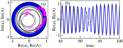
Figure 9: (Color online) Chaotic dynamics of the model (11). Black solid line shows trajectory of an oscillator; blue bold line depicts the mean field. Open circles show a snapshot of the ensemble. (a): phase portraits, (b): time dependence. Notice then when the oscillator amplitude decreases, the mean field makes an additional rotation with respect to the oscillator; thus, the time-averaged frequencies differ, as is typical for a QPS-I state.

Finally, we notice that quasiperiodic partially synchronous states can appear without synchrony-breaking transition. The most known example is the van Vreeswijk model van Vreeswijk (1996); *Mohanty-Politi-06 of leaky integrate-and-fire neurons where the quasiperiodic motion emerges from the splay state.

In summary, we have analyzed a model of nonlinearly-coupled limit-cycle oscillators and revealed two routes to two quasiperiodic states via synchrony breaking. These states appear via two different bifurcations. Moreover, we have shown the transition between QPS-I and QPS-II states, as well as domains of bistability.