NOMA Meets Finite Resolution Analog Beamforming in Massive MIMO and Millimeter-Wave Networks

Abstract

Finite resolution analog beamforming (FRAB) has been recognized as an effective approach to reduce hardware costs in massive multiple-input multiple-output (MIMO) and millimeter-wave networks. However, the use of FRAB means that the beamformers are not perfectly aligned with the users’ channels and multiple users may be assigned similar or even identifical beamformers. This letter shows how non-orthogonal multiple access (NOMA) can be used to exploit this feature of FRAB, where a single FRAB based beamformer is shared by multiple users. Both analytical and simulation results are provided to demonstrate the excellent performance achieved by this new NOMA transmission scheme.

I Introduction

Non-orthogonal multiple access (NOMA) is a promising multiple access technique for next generation wireless networks [1, 2], and has been shown to be compatible with many important 5G technologies, including massive multiple-input multiple-output (MIMO) and millimeter wave (mmWave) transmission [3, 4, 5].

A recent development in massive MIMO and mmWave networks is the use of finite resolution analog beamforming (FRAB), which reduces hardware costs [6, 7]. Analog beamforming does not alter the amplitude of a signal, but modifies its phase only, which is different from digital beamforming. The finite resolution constraint on analog beamforming is due to the fact that the number of phase shifts supported by a practical circuit is finite [6, 8]. An example for one-bit resolution analog beamforming is provided in Table I. Depending on the values of a user’s complex-valued channel coefficients, $1$ or $-1$ will be chosen as the beamformer coefficients, as shown in Table I. The reduced hardware costs of FRAB are at the expense of performance losses since the obtained beamformers are not perfectly aligned with the target users’ channels.

The purpose of this letter is to demonstrate that the characteristics of FRAB favour the use of NOMA. Consider again the example shown in Table I. To clearly show the benefit of the combination of FRAB and NOMA, the users’ channel vectors are chosen to be orthonormal, i.e., the users’ channel vectors are normalized and orthogonal to each other. The base station constructs two beams according to the channel state information (CSI) of the two users in $\mathcal{S}_{1}$. If digital beamforming with perfect resolution was used, the beamforming vector for user $1$ in $\mathcal{S}_{1}$ would be simply this user’s channel vector, and therefore this beamformer could not be used by the two users in $\mathcal{S}_{2}$, since this beamformer would be orthogonal to the two users’ channel vectors. On the other hand, if FRAB is used, the formed two beams are no longer orthogonal to the two users’ channel vectors. In fact, for the special case shown in Table I, the beamformer preferred by user $i$ in $\mathcal{S}_{1}$ is exactly the same as that of user $i$ in $\mathcal{S}_{2}$, even though the two users have orthogonal channel vectors. As a result, NOMA has been applied to ensure that all the four users can communicate concurrently. In this letter, a new NOMA transmission scheme that exploits the features of FRAB is proposed, and analytical results for the corresponding outage probabilities and diversity gains of the users are presented. The provided simulation results demonstrate not only the excellent performance of the proposed NOMA scheme, but also the accuracy of the developed analytical results. We note that the developed analytical results concerning the diversity gains are also applicable to conventional MIMO scenarios without NOMA, and hence shed light on the performance loss caused by FRAB in a general MIMO network.

TABLE I: An example for finite resolution analog beamforming

	user $1$ in $\mathcal{S}_{1}$	user $2$ in $\mathcal{S}_{1}$	user $1$ in $\mathcal{S}_{2}$	user $2$ in $\mathcal{S}_{2}$
channel	-0.19 + 0.66j	-0.49 + 0.16j	-0.27 - 0.11j	-0.33 + 0.25j
vectors	-0.06 - 0.53j	-0.35 + 0.22j	-0.06 + 0.58j	-0.45 + 0.10j
	0.34 - 0.03j	-0.10 - 0.62j	0.31 - 0.05j	-0.20 + 0.59j
	0.31 - 0.18j	-0.06 + 0.41j	0.34 - 0.60j	-0.45 - 0.15j
FRAB	-1	-1	-1	-1
beam-	-1	-1	-1	-1
formers	1	- 1	1	-1
	1	- 1	1	-1

II System Model

Consider a NOMA downlink scenario, in which the base station is equipped with $M$ antennas. Assume that there are two groups of single-antenna users in the network. Denote by $\mathcal{S}_{1}$ a set of users with strict quality of service (QoS) requirements, whose distances to the base station are denoted by $d_{yk}$ and are assumed to be fixed. Denote by $\mathcal{S}_{2}$ a set of users to be served opportunistically, and these users are uniformly distributed in a disk-shaped area with radius $r_{1}$, where the base station is at the center. Denote the distances of the users in $\mathcal{S}_{2}$ to the base station by $d_{xi}$. The $M\times 1$ channel vector of a user in $\mathcal{S}_{1}$ ($\mathcal{S}_{2}$) is denoted by $\mathbf{h}_{k}$ ($\mathbf{g}_{i}$). Two types of channel models are considered in this paper, namely Rayleigh fading and the mmWave model [7], where the mmWave channel vector is modelled as follows:

$$\mathbf{h}_{k}=\frac{a_{k}}{1+d_{yk}^{\alpha}}\begin{bmatrix}1&e^{-j\pi\theta_{k}}&\cdots e^{-j\pi(M-1)\theta_{k}}\end{bmatrix}^{T}.$$ (1)

Here, $\alpha$ denotes the path loss exponent, $\theta_{k}$ is the normalized direction, and $a_{k}$ denotes the fading attenuation coefficient. Note that for the purpose of illustration, only the line-of-sight path is considered for the mmWave model.

II-A Implementation of Finite Resolution Analog Beamforming

Suppose that the users in $\mathcal{S}_{1}$ are served via FRAB. Denote by $\mathbf{f}_{k}$ the $M\times 1$ beamforming vector for user $k$, where each element of $\mathbf{f}_{k}$ is drawn from the following vector:

$$\bar{\mathbf{f}}=\begin{bmatrix}1&e^{j\frac{2\pi}{N_{q}}}&\cdots&e^{j\frac{(N_{q}-1)2\pi}{N_{q}}}\end{bmatrix},$$ (2)

where $N_{q}$ denotes the number of supported phase shifts.

The $i$-th element of $\bar{\mathbf{f}}$ is chosen as the $m$-th element of $\mathbf{f}_{k}$ based on the following criterion:

$$i^{*}_{k,m}=\underset{i\in\{1,\cdots,N_{q}\}}{\arg\min}\quad\left|\bar{{f}}_{i}-\frac{h_{k,m}}{|h_{k,m}|}\right|^{2},$$ (3)

where $\bar{f}_{i}$ denotes the $i$-th element of $\bar{\mathbf{f}}$, and $h_{k,m}$ denotes the $m$-th element of user $k$’s channel vector.

II-B Implementation of NOMA

To reduce the system complexity, suppose that only one user from $\mathcal{S}_{2}$ will be paired with user $k$ from $\mathcal{S}_{1}$ and denote this user by user $i^{*}_{k}$. The base station sends a superposition of the messages of the two users on each beam. User $k$ in $\mathcal{S}_{1}$ treats its partner’s message as noise and decodes its own message with the following signal-to-interference-plus-noise ratio (SINR):

$$\text{SINR}_{k}=\frac{|\mathbf{h}_{k}^{H}\mathbf{f}_{k}|^{2}\alpha_{0,k}^{2}}{|\mathbf{h}_{k}^{H}\mathbf{f}_{k}|^{2}\alpha_{1,k}^{2}+\underset{l\in\mathcal{S}_{1}\setminus k}{\sum}|\mathbf{h}_{k}^{H}\mathbf{f}_{l}|^{2}+\frac{M}{\rho}},$$ (4)

where the factor $M$ in the denominator is due to the transmit power normalization, and the power allocation coefficients are denoted by $\alpha_{n,k}$. Note that $\sum^{1}_{n=0}\alpha_{n,k}^{2}=1$ and $\alpha_{0,k}\geq\alpha_{1,k}$.

By applying successive interference cancellation (SIC), user $i^{*}_{k}$ can decode its partner’s message with the following SINR: ${\text{SINR}}_{k}^{k\rightarrow i^{*}_{k}}=\frac{|\mathbf{g}_{i^{*}_{k}}^{H}\mathbf{f}_{k}|^{2}\alpha_{0,k}^{2}}{|\mathbf{g}_{i^{*}_{k}}^{H}\mathbf{f}_{k}|^{2}\alpha_{1,k}^{2}+\underset{l\in\mathcal{S}_{1}\setminus k}{\sum}|\mathbf{g}_{i^{*}_{k}}^{H}\mathbf{f}_{l}|^{2}+\frac{M}{\rho}}$. Let $\epsilon_{i}=2^{R_{i}}-1$, $i\in\{0,1\}$, where $R_{0}$ and $R_{1}$ denote the targeted data rates for user $k$ and user $i^{*}_{k}$, respectively. If ${\text{SINR}}_{k}^{k\rightarrow i^{*}_{k}}\geq\epsilon_{0}$, SIC can be carried out successfully at user $i_{k}^{*}$ and the SINR for decoding its own message is given by

$${\text{SINR}}_{k}^{i^{*}_{k}}=\frac{|\mathbf{g}_{i^{*}_{k}}^{H}\mathbf{f}_{k}|^{2}\alpha_{1,k}^{2}}{\underset{l\in\mathcal{S}_{1}\setminus k}{\sum}|\mathbf{g}_{i^{*}_{k}}^{H}\mathbf{f}_{l}|^{2}+\frac{M}{\rho}}.$$ (5)

We use the following user selection criterion:

$$i^{*}_{k}=\arg\max\{{\text{SINR}}_{k}^{k\rightarrow 1},\cdots,{\text{SINR}}_{k}^{k\rightarrow|\mathcal{S}_{2}|}\}.$$ (6)

Note that this criterion selects that user which maximizes the probability of successful intra-NOMA interference cancellation, a key stage for SIC. Since the users in $\mathcal{S}_{2}$ are served opportunistically, we allow one user from $\mathcal{S}_{2}$ to be included in more than one pair. More sophisticated user scheduling algorithms can be designed to realize fairness for the users in $\mathcal{S}_{2}$, which are not presented here due to space limitations.

III Performance Analysis

To the best knowledge of the authors, the impact of FRAB on the diversity gain has not been analyzed yet, not even for scenarios without NOMA. In order to obtain insight into the performance of the proposed NOMA scheme, in this section, we focus on the special case with $N_{q}=2$, $|\mathcal{S}_{1}|=1$, and Rayleigh fading channels. Note that $N_{q}=2$ represents the case of one-bit resolution analog beamforming [8].

III-A Performance of the User in $\mathcal{S}_{1}$

When there is a single beam, i.e., $|\mathcal{S}_{1}|=1$, the outage probability achieved by the user in $\mathcal{S}_{1}$ is given by

$$\mathrm{P}^{o}_{k}= \mathrm{P}\left(|\mathbf{h}_{k}^{H}\mathbf{f}_{k}|^{2}<\phi_{0}\right),$$

where $\phi_{i}=\frac{\frac{M\epsilon_{i}}{\rho}}{\alpha_{i,k}^{2}-\epsilon_{i}\sum^{1}_{n=i+1}\alpha_{n,k}^{2}}$, $i\in\{0,1\}$. Note that $\alpha_{i,k}^{2}>\epsilon_{i}\sum^{1}_{n=i+1}\alpha_{n,k}^{2}$ is assumed in this paper, since otherwise the outage probability is always one. In order to find the cumulative distribution function (CDF) of $|\mathbf{h}_{k}^{H}\mathbf{f}_{k}|^{2}$, the following proposition is provided first.

Proposition 1.

Consider $M$ independent and identically distributed (i.i.d.) random variables, denoted by $z_{m}$, each of which follows the folded normal distribution, i.e., $z_{m}$ is the the absolute value of a Gaussian variable with mean $0$ and variance $\frac{1}{2}$. The CDF of $z_{\sum}\triangleq\left|\sum^{M}_{m=1}z_{m}\right|^{2}$ can be approximated as follows:

$$F_{z_{\sum}}(z)\approx \frac{2^{M}}{\pi^{\frac{M}{2}}}\frac{z^{\frac{M}{2}}}{M!},$$ (7)

when $z\rightarrow 0$.

The following lemma provides an asymptotic approximation for the CDF of the effective channel gains of the user in $\mathcal{S}_{1}$.

$\mathbf{Lemma}$ 1.

For user $k$ in $\mathcal{S}_{1}$, the CDF of its effective channel gain on beam $\mathbf{f}_{k}$ can be approximated as follows:

$$F_{|\mathbf{h}_{k}^{H}\mathbf{f}_{k}|^{2}}(y)\approx \frac{2^{M}\left[y(1+d^{\alpha}_{yk})\right]^{\frac{M+1}{2}}B\left(\frac{3}{2},\frac{M}{2}\right)}{\pi^{\frac{M}{2}}(M-1)!M^{\frac{1}{2}}\Gamma\left(\frac{1}{2}\right)},$$ (8)

for $y\rightarrow 0$, where $B(\cdot)$ denotes the Beta function and $\Gamma(\cdot)$ denotes the Gamma function.

By using Lemma 1 and with some algebraic manipulations, the following corollary can be obtained.

$\mathbf{Corollary}$ 1.

For the proposed NOMA system with Rayleigh fading, user $k$ achieves a diversity gain of $\frac{M+1}{2}$.

Remark 1: With $M$ antennas at the base station, the full diversity gain for the considered scenario is $M$, but only a diversity gain of $\frac{M+1}{2}$ is achieved by the proposed scheme. This performance loss is mainly due to the use of FRAB.

Remark 2: It is important to point out that Corollary 1 is general and applicable to conventional MIMO networks without NOMA as well, since the users in $\mathcal{S}_{1}$ do not perform SIC.

III-B Performance of the User in $\mathcal{S}_{2}$

When there is a single beam, the outage probability achieved by the user in $\mathcal{S}_{2}$ is given by

$$\mathrm{P}^{o}_{i^{*}_{k}}= 1-\mathrm{P}\left(|\mathbf{g}_{i^{*}_{k}}^{H}\mathbf{f}_{k}|^{2}>\max(\phi_{0},\phi_{1})\right).$$ (9)

Note for the case of $|\mathcal{S}_{1}|=1$, the proposed user selection criterion shown in (6) simplifies to:

$$i^{*}_{k}=\arg\max\{|\mathbf{g}_{1}^{H}\mathbf{f}_{k}|^{2},\cdots,|\mathbf{g}_{|\mathcal{S}_{2}|}^{H}\mathbf{f}_{k}|^{2}\},$$ (10)

since $f(x)\triangleq\frac{x\alpha_{0,k}^{2}}{x\alpha_{1,k}^{2}+\frac{M}{\rho}}$ is a monotonically increasing function of $x$. Therefore, the CDF of $|\mathbf{g}_{i^{*}_{k}}^{H}\mathbf{f}_{k}|^{2}$ can be obtained as follows.

Denote a user randomly chosen from $\mathcal{S}_{2}$ by user $\pi(i)$, and the fading and path loss components of its composite channel gain, $\mathbf{g}_{\pi(i)}$, can be decomposed as $\mathbf{g}_{\pi(i)}=\frac{\bar{\mathbf{g}}_{\pi(i)}}{1+d^{\alpha}_{x\pi(i)}}$. Therefore, the effective fading gain of this user, $|\bar{\mathbf{g}}_{\pi(i)}^{H}\mathbf{f}_{k}|^{2}$, is exponentially distributed, since $\bar{\mathbf{g}}_{\pi(i)}$ and $\mathbf{f}_{k}$ are independent and a unitary transformation of a Gaussian vector is still Gaussian distributed. It is important to point out that $|\bar{\mathbf{g}}_{\pi(i)}^{H}\mathbf{f}_{k}|^{2}$ is exponentially distributed with parameter $\frac{1}{M}$, instead of $1$ as in [9]. By using this observation and also following steps similar to those in [9], the composite channel gain has the following approximate CDF:

$$F_{\pi(i)}(y)=\sum^{N}_{n=1}w_{n}(1-e^{-c_{n}\frac{y}{M}}),$$ (11)

where $N$ is a parameter for the Gauss-Chebyshev approximation, $w_{n}=\frac{\pi}{2N}\sqrt{1-\eta_{n}^{2}}(\eta_{n}+1)$, $\eta_{n}=\cos\left(\frac{2n-1}{2N}\pi\right)$, and $c_{n}=1+\left(\frac{r_{1}}{2}\eta_{n}+\frac{r_{1}}{2}\right)^{\alpha}$.

After applying the simplified criterion in (10) and also assuming that the users’ channels are i.i.d., the outage probability of user $i^{*}_{k}$ to decode its message delivered on beam $k$ is $\left(F_{\pi(i)}(\max(\phi_{0},\phi_{1}))\right)^{|\mathcal{S}_{2}|}$. After some algebraic manipulations, we obtain the following corollary.

$\mathbf{Corollary}$ 2.

For the proposed NOMA system with Rayleigh fading, the full diversity gain of $|\mathcal{S}_{2}|$ is achievable by the user from $\mathcal{S}_{2}$.

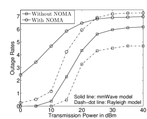
Figure 1: Outage rates achieved by the considered schemes for different channel models. $M=30$, $|\mathcal{S}_{1}|=3$, $|\mathcal{S}_{2}|=300$, $N_{q}=2$, $r_{1}=40$m, $r_{y}=r_{1}$, $\alpha=3$, $R_{0}=1$ bit per channel use (BPCU), and $R_{1}=1.5$ BPCU.

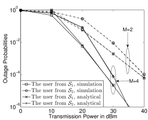
Figure 2: Outage probabilities achieved by the considered schemes for the Rayleigh fading channel model. $|\mathcal{S}_{1}|=1$, $|\mathcal{S}_{2}|=M$, $N_{q}=2$, $r_{1}=40$m, $r_{y}=\frac{r_{1}}{2}$, $\alpha=3$, $R_{0}=1$ BPCU, and $R_{1}=1$ BPCU.

IV Numerical Results

In this section, the performance of the proposed NOMA-MIMO scheme is evaluated by using computer simulations. The NOMA power coefficients are set as $\alpha_{0,k}^{2}=3/4$ and $\alpha_{1,k}^{2}=1/4$. The noise power is $-30$dBm. Without loss of generality, assume that the users in $\mathcal{S}_{1}$ lie on a circle with radius $r_{y}$, where the base station is located at its center.

Note that for the NOMA scheme, two users are served on each beam, and they have their own target data rates, $R_{0}$ and $R_{1}$, respectively. However, for the scheme without NOMA, a single user is served on each beam. For a fair comparison, the user’s targeted data rate is $R_{0}+R_{1}$ for the case without NOMA. In Fig. 1, two types of channel models, namely Rayleigh fading and the mmWave model, are considered. As can be observed from the figure, the use of NOMA can result in a significant performance gain compared to the scheme without NOMA. For example, when the transmission power of the base station is $15$dBm, the use of NOMA can offer a rate improvement of $3$ bits per channel use (BPCU) over the conventional MIMO scheme, for both considered channel models. In Fig. 2, the diversity gain achieved by the NOMA scheme is studied. To facilitate this diversity analysis, we set $|\mathcal{S}_{2}|=M$, which means that the diversity gains for the users in $\mathcal{S}_{1}$ and $\mathcal{S}_{2}$ are $\frac{M+1}{2}$ and $M$, respectively. If perfect analog beamforming is used, a diversity gain of $M$ is achievable for the user in $\mathcal{S}_{1}$ due to FRAB. From the figure, one can clearly observe the loss of diversity gain for the user from $\mathcal{S}_{1}$. Note that the curves for the analytical results match those of the simulation results, which verifies the accuracy of our analysis.

V Conclusions

In this letter, NOMA has been proposed as a means to mitigate the reduced degrees of freedom induced by FRAB in massive MIMO and mmWave networks. The developed analytical and simulation results have demonstrated the superior performance of the proposed NOMA scheme.

Appendix A Proof of Proposition 1

Recall that the probability density function (pdf) of a folded normally distributed variable is $f_{z_{m}}(x)=\frac{2}{\sqrt{\pi}}e^{-x^{2}}$. Therefore the CDF of the square of the sum of $z_{m}$ is given by

$$F_{z_{\sum},M}(z)= \frac{2^{M}}{\pi^{\frac{M}{2}}}\underset{\sum_{m=1}^{M}x_{m}<\sqrt{z}}{\int\cdots\int}\prod_{m=1}^{M}e^{-x_{m}^{2}}dx_{m},$$ (12)

where the subscript $M$ is added to show that the CDF is a function of $M$, and to facilitate the following analysis.

The proposition can be proved by using the inductive method. For the case $M=1$, the approximate expression in the proposition can be simplified as follows:

$$F_{z_{\sum,1}}(z)\approx \frac{2}{\pi^{\frac{1}{2}}}z^{\frac{1}{2}}.$$ (13)

By calculating the integral of the pdf of $z_{m}$ and applying $e^{-x}\approx 1-x$ for $x\rightarrow 0$, one can verify that (13) is a valid approximate expression for the CDF.

Assuming that the approximation is correct for the case of $M=n$, $F_{z_{\sum,n+1}}(z)$ can be expressed as follows:

$$F_{z_{\sum,n+1}}(z)= \frac{2^{n+1}}{\pi^{\frac{n+1}{2}}}\underset{\sum_{m=1}^{n+1}x_{m}<\sqrt{z}}{\int\cdots\int}\prod_{m=1}^{n+1}e^{-x_{m}^{2}}dx_{m}$$ (14)

$$= \frac{2^{n+1}}{\pi^{\frac{n+1}{2}}}\int^{\sqrt{z}}_{0}\underset{\sum_{m=1}^{n}x_{m}<\sqrt{z}-x_{n+1}}{\int\cdots\int}\prod_{m=1}^{n}e^{-x_{m}^{2}}dx_{m}$$

$$\times e^{-x_{n+1}^{2}}dx_{n+1}.$$

By using $F_{z_{\sum,n}}(z)\approx\frac{2^{n}}{\pi^{\frac{n}{2}}}\frac{(\sqrt{z})^{n}}{n!}$, $F_{z_{\sum,n+1}}(z)$ can be approximated as follows:

$$F_{z_{\sum,n+1}}(z)\approx \frac{2^{n+1}}{\pi^{\frac{n+1}{2}}}\int^{\sqrt{z}}_{0}\frac{(\sqrt{z}-x_{n+1})^{n}}{n!}e^{-x_{n+1}^{2}}dx_{n+1}$$ (15)

$$\approx \frac{2^{n+1}}{\pi^{\frac{n+1}{2}}}\int^{\sqrt{z}}_{0}\frac{(\sqrt{z}-x_{n+1})^{n}}{n!}dx_{n+1}$$

$$= \frac{2^{n+1}}{\pi^{\frac{n+1}{2}}}\frac{(\sqrt{z})^{n+1}}{(n+1)!}.$$

Therefore, the approximate expression is correct for $M=n+1$, and the proof is complete via induction.

Appendix B Proof for Lemma 1

With FRAB, the user’s effective channel gain can be expressed as follows:

$$|\mathbf{h}_{k}^{H}\mathbf{f}_{k}|^{2} =\left|\sum^{M}_{m=1}h_{k,m}e^{-j\frac{(i^{*}_{k,m}-1)2\pi}{N_{q}}}\right|^{2}.$$ (16)

When $N_{q}=2$, we separate the real and imaginary parts of the user’s channel as follows:

$$|\mathbf{h}_{k}^{H}\mathbf{f}_{k}|^{2} =\left|\sum^{M}_{m=1}(h_{k,m,real}+jh_{k,m,imag})\bar{f}_{i^{*}_{k,m}}\right|^{2}$$ (17)

$$=\left|\sum^{M}_{m=1}(|h_{k,m,real}|+j\text{sign}(h_{k,m,real})h_{k,m,imag})\right|^{2},$$

where $\text{sign}(\cdot)$ is the sign operation. This separation leads to the following expression:

$$|\mathbf{h}_{k}^{H}\mathbf{f}_{k}|^{2}= \left|\sum^{M}_{m=1}\bar{h}_{m}\right|^{2}+\left|\bar{h}_{0}\right|^{2},$$ (18)

where $\bar{h}_{0}=\sum^{M}_{m=1}\text{sign}(h_{k,m,real})h_{k,m,imag}$ and $\bar{h}_{m}=|h_{k,m,real}|$. Note that $\text{sign}(h_{k,m,real})$ is independent of $|h_{k,m,real}|$, because the phase and the amplitude of a complex Gaussian random variable are independent. Therefore, $\left|\sum^{M}_{m=1}\bar{h}_{m}\right|^{2}$ and $\left|\bar{h}_{0}\right|^{2}$ are independent.

Define $z_{0}=|\bar{h}_{0}|^{2}$ whose pdf can be easily obtained as follows. Recall that the sum of i.i.d. Gaussian random variables is still a Gaussian variable, which means $\bar{h}_{0}$ is Gaussian with zero mean and variance $\frac{M}{2(1+d_{yk}^{\alpha})}$. Therefore, the CDF of $z_{0}$ is given by

$$F_{z_{0}}(z)=\frac{\gamma\left(\frac{1}{2},\frac{(1+d_{yk}^{\alpha})z}{M}\right)}{\Gamma\left(\frac{1}{2}\right)},$$ (19)

and the pdf is $f_{z_{0}}(z)=\frac{dF_{z_{0}}(z)}{dz}$, where $\gamma(x,y)$ denotes the incomplete Gamma function.

Therefore, the CDF of $|\mathbf{h}_{k}^{H}\mathbf{f}_{k}|^{2}$ can be expressed as follows:

$$F_{|\mathbf{h}_{k}^{H}\mathbf{f}_{k}|^{2}}(y) =\underset{x+z<y}{\int\int}f_{z_{0}}(z)f_{\bar{z}_{\sum}}(x)dzdx.$$ (20)

According to Proposition 1, when $z\rightarrow 0$, the pdf of $\bar{z}_{\sum}\triangleq\left|\sum^{M}_{m=1}\bar{h}_{m}\right|^{2}$ can be approximated as follows:

$$f_{\bar{z}_{\sum}}(x)\approx\frac{2^{M-1}(1+d_{yk}^{\alpha})^{\frac{M}{2}}}{\pi^{\frac{M}{2}}}\frac{x^{\frac{M-2}{2}}}{(M-1)!}.$$ (21)

Therefore, when $y\rightarrow 0$, we have the following approximation:

$$F_{|\mathbf{h}_{k}^{H}\mathbf{f}_{k}|^{2}}(y)= \int^{{y}}_{0}f_{\bar{z}_{\sum}}(x)\int^{y-x}_{0}f_{z_{0}}(z)dzdx$$ (22)

$$\approx \int^{{y}}_{0}\frac{2^{M-1}(1+d_{yk}^{\alpha})^{\frac{M}{2}}}{\pi^{\frac{M}{2}}}\frac{x^{\frac{M-2}{2}}}{(M-1)!}F_{z_{0}}(y-x)dx.$$

Note that when $x\rightarrow 0$, the CDF in (19) can be approximated as follows:

$$F_{z_{0}}(z)\approx\frac{2(1+d_{yk}^{\alpha})^{\frac{1}{2}}z^{\frac{1}{2}}}{M^{\frac{1}{2}}\Gamma\left(\frac{1}{2}\right)}.$$ (23)

Therefore, the following approximation can be obtained:

$$F_{|\mathbf{h}_{k}^{H}\mathbf{f}_{k}|^{2}}(y)\approx \frac{2^{M}(1+d_{yk}^{\alpha})^{\frac{M+1}{2}}\int^{{y}}_{0}x^{\frac{M-2}{2}}(y-x)^{\frac{1}{2}}dx}{\pi^{\frac{M}{2}}(M-1)!M^{\frac{1}{2}}\Gamma\left(\frac{1}{2}\right)}.$$

Using the definition of the Beta function in the above expression, the lemma is proved.

References

• [1] Z. Ding, Y. Liu, J. Choi, Q. Sun, M. Elkashlan, C.-L. I, and H. V. Poor, “Application of non-orthogonal multiple access in LTE and 5G networks,” IEEE Commun. Mag., vol. 55, no. 2, pp. 185–191, Feb. 2017.
• [2] L. Song, Y. Li, Z. Ding, and H. V. Poor, “Resource management in non-orthogonal multiple access networks for 5G and beyond,” IEEE Networks, (to appear in 2017) Available on-line at arxiv.org/abs/1610.09465.
• [3] Z. Ding and H. V. Poor, “Design of massive-MIMO-NOMA with limited feedback,” IEEE Signal Process. Lett., vol. 23, no. 5, pp. 629–633, May 2016.
• [4] X. Liu and X. Wang, “Efficient antenna selection and user scheduling in 5G massive MIMO-NOMA system,” in Proc. IEEE Veh. Tech. Conf., Nangjing, China, May 2016.
• [5] Z. Ding, P. Fan, and H. V. Poor, “Random beamforming in millimeter-wave NOMA networks,” IEEE Access, (to appear in 2017).
• [6] A. Alkhateeb, Y. H. Nam, J. Zhang, and R. W. Heath, “Massive MIMO combining with switches,” IEEE Wireless Commun. Lett., vol. 5, no. 3, pp. 232–235, Jun. 2016.
• [7] X. Gao, L. Dai, Y. Sun, S. Han, and C.-L. I, “Machine learning inspired energy-efficient hybrid precoding for mmWave massive MIMO systems,” in Proc. IEEE Int. Conf. on Commun., Paris, France, May 2017.
• [8] H. Yang, F. Yang, S. Xu, Y. Mao, M. Li, X. Cao, and J. Gao, “A 1-bit 10X10 reconfigurable reflectarray antenna: Design, optimization, and experiment,” IEEE Trans. Antennas Propag., vol. 64, no. 6, pp. 2246–2254, Jun. 2016.
• [9] Z. Ding, Z. Yang, P. Fan, and H. V. Poor, “On the performance of non-orthogonal multiple access in 5G systems with randomly deployed users,” IEEE Signal Process. Lett., vol. 21, no. 12, pp. 1501–1505, Dec. 2014.