Finite-size-induced transitions to synchrony in oscillator ensembles with nonlinear global coupling

Abstract

We report on finite-sized-induced transitions to synchrony in a population of phase oscillators coupled via a nonlinear mean field, which microscopically is equivalent to a hypernetwork organization of interactions. Using a self-consistent approach and direct numerical simulations, we argue that a transition to synchrony occurs only for finite-size ensembles, and disappears in the thermodynamic limit. For all considered setups, that include purely deterministic oscillators with or without heterogeneity in natural oscillatory frequencies, and an ensemble of noise-driven identical oscillators, we establish scaling relations describing the order parameter as a function of the coupling constant and the system size.

Collective synchronization phenomena are abundant in complex nonlinear systems, and onset of synchrony can be typically treated as a nonequilibrium phase transition. The Kuramoto model Kuramoto (1975); *Acebron-etal-05 of globally coupled phase oscillators is the simplest paradigmatic system, where this transition can be explored nearly in full details Strogatz (2000); *Ott-Antonsen-08, also a relation to equilibrium transitions is well studied Gupta et al. (2014). This model is universally applicable for ensembles of weakly coupled oscillators, possessing harmonic phase sensitivity (like, e.g., Josephson junctions Wiesenfeld et al. (1996)). In many cases one, however, needs to go beyond such a simple setup, allowing for couplings that include higher harmonics, this is relevant for electrochemical oscillators Kiss et al. (2005) and $\varphi$-Josephson junctions Goldobin et al. (2011). Moreover, as suggested in Rosenblum and Pikovsky (2007) and experimentally realized in Temirbayev et al. (2012); *Temirbayev_et_al-13, coupling terms can be nonlinear functions of the order parameters (mean fields).

In this letter we describe nontrivial properties of the synchronization transition in a model with simple nonlinear coupling, where the coupling is at the second harmonics of the phase, but is proportional to the the square of the Kuramoto order parameter. We will show that such an interaction on a microscopic level represents a fully connected hypernetwork. By performing the analysis in the thermodynamic limit, we will demonstrate, that for deterministic ensembles the asynchronous state with a uniform distribution of the phases never loses stability; for noisy oscillators it is possible to show that such an asynchropnous state is the only stationary solution. Nevertheless, direct numerical simulations of finite pupulations yield partially synchronous regimes. These regimes can be called finite-size-induced one; the main goal of this paper is to clarify their nature. Our main tool is the analysis of scaling of partial synchrony with the system size. We will establish scaling properties of this finite-size-induced transition for different setups: identical purely deterministic oscillators, identical noisy oscillators, and deterministic non-identical ensemble (the latter setup is mostly close to the Kuramoto model). From these scaling properties it follows, that in the thermodinamic limit the characteristic value of the observed order parameter tends to zero, while the critical value of the coupling strength at which partial synchrony is observed, diverges. Thus, this transition to synchrony can be called finite-size-induced one.

Let us start with formulation of general phase equations for an ensemble of nonlinear oscillators coupled via mean fields. In the limit of weak coupling (or weak external forcing), the dynamics of each oscillator can be described by its phase $\phi(t)$ via the phase response function $S(\phi)$:

$$\dot{\phi}=\Omega+\omega+S(\phi)F,$$

here $\Omega$ stands for the population mean natural frequency and $\omega$ is an individual deviation from the mean. The term $F$ is an overall force produced by mean field coupling, i.e. it is a general function of mean fields (Daido order parameters Daido (1993); *Daido-96) $Z_{k}=\langle e^{ik\phi}\rangle$ (here $\langle\rangle$ means averaging over the ensemble) which can be represented as an expansion $F=\sum_{k,m}h_{k,m}(Z_{k})^{m}$ (where $h_{k,m}$ are constants). Next, let us introduce a slowly varying phase $\varphi(t)=\phi(t)-\Omega t$ and the corresponding slow order parameters $\bar{Z}_{k}=\langle e^{ik\varphi}\rangle=Z_{k}e^{-ik\Omega t}$. Using a Fourier representation of the phase response function $S(\phi)=\sum_{n}s_{n}e^{-in\phi}$ we get the following general equation for the slow phase:

$$\dot{\varphi}=\omega+\sum_{n,k,m}s_{n}e^{-in\varphi}h_{k,m}\bar{Z}_{k}^{m}e^{i(km-n)\Omega t}.$$ (1)

Performing an averaging of the equation (1) over the fast time scale $\Omega^{-1}$ is equivalent to keeping only terms on the r.h.s. that do not contain explicit time dependence $\sim e^{ij\Omega t}$, i.e. we have to set $n=km$:

$$\dot{\varphi}=\omega+\sum_{k,m}s_{km}e^{-ikm\varphi}h_{k,m}\bar{Z}_{k}^{m}.$$ (2)

This is the general form of the phase equation derived for a weakly coupled oscillatory ensemble with generically nonlinear (due to terms with $m>1$) mean-field interaction (cf. Rosenblum and Pikovsky (2007)). Recall that the simplest case where $n=k=m=\pm 1$ gives us the term $\sim\bar{Z_{1}}e^{-i\varphi}$, and (2) reduces to the standard Kuramoto-Sakaguchi model Sakaguchi and Kuramoto (1986). Considering further terms with $n=km=\pm 2$, we get a generalized bi-harmonic coupling $\sim s_{1}h_{1,1}\bar{Z}_{1}e^{-i\varphi}+(s_{2}h_{2,1}\bar{Z}_{2}+s_{2}h_{1,2}\bar{Z}_{1}^{2})e^{-i2\varphi}$ on the r.h.s of the system (2). The case where the bi-harmonic coupling depends linearly on the order parameters ($h_{1,2}=0$) was extensively studied in Refs. Komarov and Pikovsky (2013); *Komarov-Pikovsky-14; *Vlasov-Komarov-Pikovsky-15.

In this letter we focus on the effects produced by purely nonlinear second-harmonic coupling $s_{1}=h_{2,1}=0$ (see Skardal et al. (2011) for the analysis of linear second-harmonic coupling $s_{1}=h_{1,2}=0$) and show that it is responsible for finite-size induced transitions to synchrony with nontrivial scaling on the ensemble size. We will demonstrate that while synchrony disappears in the thermodynamic limit, it is observed for finite ensembles. Thus, throughout this paper we consider the following model, where also external noise is taken into account for completeness:

$$\dot{\varphi}_{k}=\omega_{k}+\varepsilon R^{2}\sin(2\Theta-2\varphi_{k})+\sqrt{D}\eta_{k}(t),\ \ \ k=1,...,N.$$ (3)

Here we denote $Re^{i\Theta}=\bar{Z}_{1}=N^{-1}\sum_{k=1}^{N}e^{i\varphi_{k}}$, $N$ is the size of population, and the noise is Gaussian delta-correlated $\langle\eta_{k}(t)\eta_{m}(t-t_{0})\rangle=\delta_{km}\delta(t-t_{0})$. Qualitatively, nontrivial features of this model can be understood as follows. Because the interaction is proportional to the second harmonics of the phase $\sim\sin 2\varphi$, it supports formation of two clusters, with phase difference $\pi$. However, the coupling term is determined by the order parameter $R$ which vanishes if two symmetric clusters are formed and is non-zero only due to asymmetry of the clusters. This asymmetry, as we shall demonstrate below, is due to finite-size fluctuations at the initial stage when the clusters are formed from the disorder.

Before proceed with the main analysis, we discuss physical relevance of the model (3). First, the purely second-harmonic coupling ($s_{1}=0$) appears when the force acts on nearly harmonic oscillators parametrically (a typical example here are mechanical pendula suspended on a vertically oscillating common beam). Another situation where the second harmonic in $S(\phi)$ dominates is that of period-doubled oscillations. Noteworthy, due to nonlinear coupling model (3) represents a hypernetwork Wang, Jian-Wei et al. (2010); *Bilal-Ramaswamy-14 of oscillators. Indeed, substituting the expression for the mean field in (3), one can see that the microscopic coupling terms can be written as $\sim\sin(\varphi_{l}+\varphi_{m}-2\varphi_{k})$. This means that effective interactions are not pairwise (as in the standard Kuramoto model and its numerous generalizations) but via triplets; this is exactly the definition of a hypernetwork coupling structure.

Furthermore, it is worth discussing the rôle of different order parameters in the problem. The order parameter $\bar{Z}_{1}$ governs the force acting on the oscillators and is therefore of major importance. Because this force contains the second harmonics only ($\sim\sin 2\varphi_{k}$), the appearing order is of “nematic” type and corresponds to large absolute values of the order parameter $\bar{Z}_{2}$; at these states the order parameter $R=|\bar{Z}_{1}|$ may be small. In the disordered, asynchronous states both order parameters $\bar{Z}_{1,2}$ are small.

Linear stability analysis of a disordered state ($R=0$) in model (3) is straightforward, beacuse coupling is nonlinear in $R$ and thus does not contribute. The solution is the same as for the Kuramoto model with vanishing coupling Strogatz and Mirollo (1991); *Crawford-Davies-99: the disordered state is either neutrally (without noise $D=0$), or asymptotically stable. Thus, all the transitions described below are due to nonlinear and finite-size effects.

We start with the simplest case where all oscillators have identical frequencies ($\omega_{k}=0$) and are not affected by noise ($D=0$). In this case, for any $Re^{i\Theta}=const\neq 0$ there are two stable positions for the phases: $\varphi_{1}=\Theta$ and $\varphi_{2}=\Theta+\pi$. Any distribution $(n_{1},n_{2})$ with $n_{1}>N/2$ oscillators in the first state is possible, with order parameter

$$R=2n_{1}/N-1\;.$$ (4)

Only the symmetric distribution with $n_{1}=N/2$ is not a solution, because the mean field vanishes. Therefore, in the thermodynamic limit $N\to\infty$, the stationary two-cluster distributions can be written as

$$\rho(\varphi)=S\delta(\varphi-\Theta)+(1-S)\delta(\varphi-\Theta+\pi),$$ (5)

with an arbitrary indicator constant $S\in\big{(}\frac{1}{2},1\big{]}$, the order parameter is $R=2S-1$ and $\Theta$ is arbitrary.

A nontrivial question here is: which of possible synchronous states establishes if one starts from a fully disordered initial configuration with uniformly distributed initial phases $0\leq\varphi_{k}<2\pi$. Numerically obtained distributions of the final states, for different sizes $N$, are shown in Fig 1(a). Here the order parameter $R$ can attain only discrete values according to (4), and $p$ are probabilities of these states. Remarkably, these distributions collapse perfectly after rescaling $R\to R\sqrt{N}$, $p\to p\sqrt{N}$, as is shown in Fig. 1(b). This means that the stationary order parameter scales as $R\sim N^{-1/2}$, i.e. it disappears in the thermodynamic limit. To this scaling corresponds also the scaling of the characteristic transient time from initial disorder to a final synchronous configuration: as one can see from (3), this time is $\sim R^{-2}\sim N$, what is confirmed by numerics (not shown).

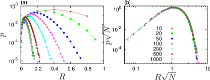
Figure 1: (color online) The histograms of the two-cluster states which result from the disordered initial conditions $R\approx 0$, for different ensemble sizes from $N=10$ to $N=1000$. Panel (b) shows scaling $p\sim N^{-1/2}F(RN^{1/2})$; dashed line is a fitting curve $F(x)=5.2x^{3}\exp[-1.45x^{3/2}]$. Theoretical derivation of this scaling relation remains an unsolved problem.

Next, we consider the case when the oscillators have different natural frequencies $\omega_{k}$ and are not affected by noise $D=0$. We assume a Gaussian distribution $g(\omega)=(2\pi)^{-1/2}e^{-\omega^{2}/2}$ (without loss of generality the width of the distribution is set to 1 and the mean frequency to 0). First, following Refs. Komarov and Pikovsky (2013); *Komarov-Pikovsky-14; *Vlasov-Komarov-Pikovsky-15, we find stationary solutions in the thermodynamical limit by virtue of a self-consistent scheme. We will see, that although the analysis of the thermodynamic limit does not provide a transition to partial synchrony, it allows us to find states close to that observed in simulations of finite systems. For the sake of brevity of presentation we restrict to symmetric, non-rotating solutions only, then without loss of generality one can set $\Theta=0$. For such states the conditional distribution density $\rho(\varphi|\omega)$ is stationary, and the order parameter can be defined as follows:

$$R=\iint d\omega\,d\varphi\,g(\omega)\rho(\varphi|\omega)\cos\varphi.$$ (6)

It is convenient to introduce an auxiliary parameter $A=\varepsilon R^{2}$ (the overall amplitude of the coupling function) and the rescaled frequency $x=\omega/A$. It easy to see from (3) that all the oscillators can be divided into those locked by the mean field ($|x|<1$) and the unlocked (rotating) ones $(|x|>1)$. The distribution of the latter ones is inversely proportional to the phase velocity $\rho_{u}(\varphi|x)=C|A(x-\sin(2\varphi))|^{-1}$ (here $C$ is a normalization constant) and, because of the symmetry, it does not contribute to the order parameter in (6). The distribution of the locked oscillators $\rho_{L}(\varphi|x)$ is in fact the same as in (5), but frequency-dependent:

$$\rho_{L}(\varphi|x) =S(x)\delta(\varphi-\Phi)+(1-S(x))\delta(\varphi-\Phi-\pi)$$ (7)

where $\Phi(x)={\arcsin(x)}/{2}$. Similar to the case of identical oscillators, the indicator function $S(x)$ is arbitrary (due to assumed symmetry we restrict ourselves to the case $S(x)=S(-x)$, asymmetric functions lead generally to rotating solutions), it describes redistribution of oscillators between two stable branches $\varphi=\Phi(x)$ and $\varphi=\Phi(x)+\pi$. Below we consider the simplest case of constant indicator function $S(x)=\sigma\in\big{(}\frac{1}{2},1]$. In order to get the final closed self-consistent scheme, we need to substitute the distribution function (7) into the definition of the order parameter (6). This yields the order parameter $R$ as a function of the coupling constant $\varepsilon$ in a parametric (in dependence on auxillary parameter $A$) analytic form:

$$R =A(2\sigma-1)H(A),\ \ \ \varepsilon=AR^{-2},$$ (8)

$$H(A) =\int_{-\frac{\pi}{4}}^{\frac{\pi}{4}}2\cos\varphi\cos 2\varphi g(A\sin 2\varphi)d\varphi.$$

Figure 2(a) illustrates stationary solutions $R(\varepsilon)$ at different indicator constants $\sigma$. The black curves denote the main solution at $\sigma=1$. At a critical coupling $\varepsilon_{c}\approx 2.17$ two branches, stable (black solid) and unstable (dashed line) arise (stability is determined by direct finite-size numerical simulations). Note that these lines are separated from the disordered solution $R=0$, although $R\sim\varepsilon^{-1}$ as $\varepsilon\to\infty$ at the unstable branch. Solutions for $\sigma<1$ can be easily found from the rescaling of the main dependence (at $\sigma=1$) according to (8). So, the curves $R(\varepsilon)$ at $\sigma<1$ have qualitatively similar structure, however, they are shifted to larger values of $\varepsilon$ for smaller values of $\sigma$ (see dotted red lines in Fig. 2(a)). In particular, the critical points scale as $R_{c}(\sigma)=R_{c}(0)\left(\frac{\varepsilon_{c}(1)}{\varepsilon_{c}(\sigma)}\right)^{1/2}$. This blue bold line in Fig. 2(a) together with the black solid line at $\sigma=1$ define the region of possible synchronous solutions, characterized by different indicator constants $\sigma$.

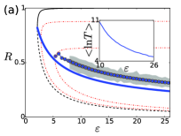
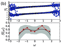
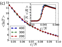
Figure 2: (color online) (a) Black solid and dashed curves: solution of the self-consistent equations (8) for $\sigma=1$. Blue bold curve - the bifurcation line where two branches of synchronous solutions appear for different $\sigma$. Blue markers: mean value of $R$ obtained from direct numerical simulation of (3) with $N=200$ and initial conditions in the incoherent state. Dotted red lines denote solution of self-consistent equation (8) for $\sigma=0.94$ and $\sigma=0.82$. The inset show the averaged lifetime $T$ of the incoherent state for the finite-size ensemble. (b) The top panel shows coordinates of phase $\varphi$ as a function of internal frequency $\omega$ in the stationary synchronous state (the data is shown for 1000 different simulations at $\varepsilon=15$, $N=200$). The bottom panel depicts function $S(\omega)$ in the range where the oscillators are locked and form two distinct stable branches. The black solid curve stands for averaged values of $S(\omega)$, the gray area denotes the standard deviation, and the red markers depict one particular realization. In order to calculate $S(\omega)$, the range $\omega\in[-2,2]$ was split into $m$ subintervals. In each subinterval we calculate the ratio of oscillators, located at different branches. For averaged black curve we use $m=20$, for red curve $m=10$. (c) The dependence of the averaged lifetime $T$ of the incoherent state is shown for different system sizes $N$. The inset depicts the averaged value of order parameter $R$ obtained from finite-size finite-time ($T_{max}=10^{6}$) simulations of the system (3).

It is worth mentioning that the incoherent solution $R=0$ exists at any value of coupling $\varepsilon$ and it is always stable in the thermodynamical limit. However, in the finite-size simulations of the system (3), we found that the incoherent state has a finite lifetime: after a long transient a synchronous state from the described above solution family (i.e. between the blue bold and black solid curves in Fig. 2(a)) sets on, and this state remains further stable. Blue markers in the Fig. 2(a) denote averaged value of $R$ obtained from direct numerical simulations of (3) with $N=200$. The averaging was performed over $\sim 1000$ distinct simulation runs (until final time $T_{max}=10^{6}$) with disordered initial conditions. The final state to which the system jumps from the incoherence is not always the same and has a deviation range depicted by the gray area in Fig. 2(a).

A more detailed description of the final synchronous state is presented in the Fig. 2(b). Here the top panel shows dependence of the phases $\varphi$ on the internal frequency $\omega$. The area in the center clearly shows two stable branches of locked oscillators. Outside this area one can see the clouds of points, which depict unlocked oscillators. The unlocked phases rotate in relation to the mean field phase, and, therefore, constitute an asynchronous part of the ensemble. The bottom panel shows statistics of the function $S(\omega)$, which is calculated in the range $\omega\in[-2,2]$ where oscillators are typically locked to the mean field. The function has certain profile depicted in the bottom panel of the Fig. 2(b). As one can see, the distribution of locked oscillators over the branches remains close to a constant value in the center of the $\omega$ range, however, it drops significantly close to the boundaries of the coherent region.

The averaged lifetime $T$ of the incoherent state drastically increases with decrease of coupling constant $\varepsilon$, what is shown in the inset of Fig. 2(a). Thus, below $\varepsilon\approx 7$ it is impossible to collect any reasonable statistics with a finite simulation time $T_{max}=10^{6}$. However, even for relatively small values of $\varepsilon$, the transition from the incoherent state is possible, what is shown by the blue markers to the left of they gray colored area.

It is instructive to characterize this finite-size induced transition to synchrony in dependence on the system size $N$. The dependence of averaged lifetime $T$ on the rescaled coupling $\varepsilon/N$, plotted in the Fig. 2(c), demonstrates a nice collapse of data points. This scaling follows from the fact that the characteristic amplitude of the coupling term is $\varepsilon R^{2}$ and $R\sim N^{-1/2}$ in the disordered state. Furthermore, in the inset of the Fig. 2(c) we show a rescaled order parameter, obtained at the end of a fixed integration time $T_{max}$; one can see that it scales as $\langle R\rangle\sim N^{-1/2}f(\varepsilon N)$, what can be explained as follows. For sufficiently small values of the coupling the system always exhibits finite-size fluctuations $R\sim N^{-1/2}$ and remains in the asynchronous state. With increase of $\varepsilon$, the transition to synchronous state becomes more probable what leads to an increase of the averaged final value of $R$. The upper branch reflects the scaling of the lowest border of synchronous states $R\sim\varepsilon^{-2}$ mentioned above. Note that the critical value of coupling resulting from this scaling is $\varepsilon\sim N$, so the transition effectively disappears in the thermodynamic limit.

Finally, we describe the finite-size-induced transitions to synchrony in the ensemble of identical oscillators ($\omega_{k}=0$) with noise $D\neq 0$ (3). Without lose of generality, we can take $D=1$, so that the only parameters are $\varepsilon$ and $N$. In the thermodynamic limit, when $N\to\infty$, the system does not have any non-trivial coherent solution, because due to the symmetry $\varphi\to\varphi+\pi$ of the coupling function, the stationary density $\rho$ that follows from the Fokker-Planck equation is also symmetric (in the small noise limit it tends to (5) with $S=1/2$), thus the only stationary solution is the incoherent one with $R=0$. However, similar to the situations described above, for small system sizes $N$ a transition to synchronous two-cluster configurations is observed (cf. Ref. Pikovsky et al. (1994)). In contradistinction to the noise-free case, here also back transitions to disorder are possible due to noise, so that at a long run the process looks like an intermittent order-disorder dynamics.

Qualitatively, this dynamics can be understood as effect of noise on the multiplicity of synchronous states described for the noise-free case above (cf. discussion around Eq. (5)): due to small noise now transitions between these states $(n_{1},n_{2})\to(n_{1}\pm 1,n_{2}\mp 1)$ occur. The transitions rates one can estimate using the Kramers’ formula, they are exponentially small in the potential barrier which is $2\varepsilon R^{2}$ where $R=|2n_{1}/N-1|$. For small $R$, the Kramers’ rate does not apply, here one can phenomenologically set the transition rate to a constant. As a result, one obtains for the order parameter $R$ a random walk model, which can be described by the corresponding master equation. Without going into details, which will be presented elsewhere, we present here the main results of this statistical model. The stationary distribution (Fig. 3(a)) shows a transition to synchrony at $\varepsilon_{c}\approx 0.35N$, so that for larger couplings we get $R\approx 1$, while below this threshold only finite-size fluctuations around disordered state with $R\sim N^{-1/2}$ are observed. The characteristic time scale of the time evolution from asynchrony to synchrony is however extremely large, because the Kramers’ rate at large $R$ is exponentially small. Thus, direct simulations of finite ensembles, started from a disordered state and performed over a finite time interval $T_{max}$, allow to reveal only order parameters for which $\exp{\varepsilon R^{2}}\lesssim T_{max}$, thus $R_{max}\sim(\ln T_{max})^{1/2}\varepsilon^{-1/2}$. At this stage the evolution becomes effectively “frozen”. We illustrate this in Fig. 3(b): only for $N\lesssim 15$ one observes a saturation of the order parameter as predicted by the random walk model, while for larger $N$, values of order parameter close to one are never achieved during available integration times. Of course, if one starts from a state with $R$ close to one, it remains practically frozen as well.

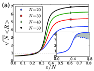
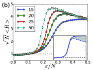
Figure 3: (color online) Dependence of the order parameter $R$ on the rescaled coupling constant for identical oscillators with noise. (a) Stationary state in the master equation as described in text. The inset shows the difference between the steady state (solid line) and the one evolving from the disordered state at finite time (dashed line) for $N=20$. (b) Direct numerical simulations of ensemble  (3) (observation time $T_{max}=10^{6}$). The inset shows results for system size $N=25$, but for different initial conditions (solid line: starting from a state with large $R$, dashed: starting from the disordered state).

Summarizing, in this letter we considered a model of oscillators, globally coupled via a nonlinear function (in our case, square) of the Kuramoto mean field. Equivalently, on the microscopic level such a coupling can be described as a fully connected hypernetwork. While the disordered state remains stable in the linear approximation and in the thermodynamic limit, a transition to synchrony is observed due to finite-size effects: the characteristic critical coupling parameter value scales typically as $\varepsilon\sim N$, also the transient time from disorder to order diverges as $N\to\infty$. For the deterministic ensembles we demonstrated scaling properties of the transition in form of dependence of the order parameter on the coupling strength and the ensemble size. For the noisy case, the system demonstrates effective breaking of ergodicity, being trapped in frozen metastable states due to exponentially small hopping rates. While we focused on the purely quadratic in mean field coupling, the described framework allows one also to consider a general combination of linear and nonlinear couplings. The approach based on the master equation provides a framework for a description of finite-size transitions not only in the context of phase oscillator networks, but in other types of mean-field coupled systems demonstrating finite-size-induced transition Pikovsky et al. (1994).