Elastic properties and mechanical tension of graphene

Abstract

Room temperature simulations of graphene have been performed as a function of the mechanical tension of the layer. Finite-size effects are accurately reproduced by an acoustic dispersion law for the out-of-plane vibrations that, in the long-wave limit, behaves as $\rho\omega^{2}=\sigma k^{2}+\kappa k^{4}$. The fluctuation tension $\sigma$ is finite ($\sim 0.1$ N/m) even when the external mechanical tension vanishes. Transverse vibrations imply a duplicity in the definition of the elastic constants of the layer, as observables related to the real area of the surface may differ from those related to the in-plane projected area. This duplicity explains the variability of experimental data on the Young modulus of graphene based on electron spectroscopy, interferometric profilometery, and indentation experiments.

I Introduction

Graphene is a solid surface in three-dimensional (3D) space.(Amorim et al., 2016) The area per atom, $A$, is a thermodynamic property difficult to be measured. In fact the accessible observable is its projection, $A_{p}$, onto the mean plane of the membrane, with $A_{p}\leq A$. The equality is achieved in a strictly plane layer. The existence of two different areas, $A$ and $A_{p}$, suggests a duplicity of physical properties. For example, the negative thermal expansion coefficient of graphene refers only to $A_{p}$, while the thermal expansion of $A$ is positive.(Pozzo et al., 2011; Herrero and Ramírez, 2016) An internal tension conjugated to the actual membrane area $A$ should be distinguished from a mechanical frame tension, $\tau$, conjugated to the projected area, $A_{p}$. It is the tension $\tau$, the lateral force per unit length at the boundary of $A_{p}$, the magnitude that defines the thermodynamic ensemble in computer simulations.(Fournier and Barbetta, 2008) $\tau$ is measurable in fluid membranes by micropipette aspiration experiments.(Evans and Rawicz, 1990) In addition, graphene elastic moduli, as the bulk or Young modulus, may have different values if they are defined from fluctuations of either $A$ or $A_{p}$. To avoid misunderstandings one should specify unambiguously the kind of variable to which one is referring.

Differences between $A$ and $A_{p}$ originate from the existence of ripples or wrinkles, that are a manifestation of the perpendicular acoustic (ZA) vibrational modes of the layer. The harmonic long-wave limit ($k\rightarrow 0$) of the ZA phonon dispersion is $\rho\omega^{2}=\sigma k^{2}+\kappa k^{4}.$ Here $\rho$ is the atomic mass density and $\kappa$ the bending rigidity of the layer. $\sigma$ is the fluctuation tension,(Fournier and Barbetta, 2008; Tarazona et al., 2013) that depends on the applied mechanical tension as $\sigma=-\tau.$ (de Andres et al., 2012) The anharmonicity of the out-of-plane fluctuations causes a renormalization of the harmonic parameters. Room temperature simulations of free standing graphene at zero mechanical tension $(\tau=0)$ reveal a finite fluctuation tension of $\sigma_{0}\sim 0.1$ N/m.(Ramírez et al., 2016) This result agrees with analytical treatments of anharmonic effects by perturbation theory,(Amorim et al., 2014; Michel et al., 2015; Adamyan et al., 2016) with a study of the coupling between vibrational and electronic degrees of freedom by density functional calculations, (Kumar et al., 2010) and with the analysis of symmetry constraints in the phonon dispersion curves of graphene.(Falkovsky, 2008) All these studies are compatible with an anharmonic relation between fluctuation and mechanical tensions as $\sigma=\sigma_{0}-\tau.$ However, the long-wave limit predicted by a membrane model with anomalous exponents deviates from this relation.(Los et al., 2016)

In this paper, the anharmonicity of a free standing graphene layer is studied by molecular dynamics (MD) simulations in the $N\tau T$ ensemble ($N$ being the number of atoms in the simulation cell and $T$ the temperature). The fluctuation tension, $\sigma$, and the bending rigidity, $\kappa$, of the layer are studied at $300$ K as a function of both tensile $(\tau<0)$ and compressive $(\tau>0)$ stresses. The analytic long-wave limit, $\rho\omega^{2}=\sigma k^{2}+\kappa k^{4}$, of the ZA phonons allows us the formulation of a finite-size correction to the simulations. The amplitude of transverse fluctuations, $h^{2}$, the projected area, $A_{p},$ and the bulk moduli, $B$ and $B_{p}$, associated to the fluctuation of the areas $A$ and $A_{p}$, are studied in the thermodynamic limit ($N\rightarrow\infty)$ as a function of $\tau$. The bulk moduli ($B$ and $B_{p}$) are observables with different behavior. While $B$ remains finite for all studied tensions, $B_{p}\rightarrow 0$ for a critical compressive tension, $\tau_{c}$. This is the maximum tension that a planar layer can sustain, before making a transition to a non-planar wrinkled structure. Our findings provide light into the variability of experimental data on the Young modulus of graphene based either on high-resolution electron energy loss spectroscopy (HREELS) (Politano and Chiarello, 2015), on interferometric profilometery,(Nicholl et al., 2015) or on indentation experiments with an atomic force microscope (AFM).(Lee et al., 2008, 2013; Lopez-Polin et al., 2015)

II Computational method

II.1 MD simulations

The simulations are performed in the classical limit with a realistic interatomic potential LCBOPII.(Los et al., 2005) The original parameterization was modified to increase the $T\rightarrow 0$ limit of the bending rigidity from $1.1$ eV to a more realistic value, $\kappa=1.5$ eV.(Ramírez et al., 2016; Lambin, 2014) A supercell $(N_{x},N_{y})$ of a 2D rectangular cell $(\mathbf{a},\mathbf{b})$ including 4 carbon atoms was employed with 2D periodic boundary conditions.(Ramírez et al., 2016) The supercell is chosen so that $N_{x}a\sim N_{y}b$. Runs consisted of $10^{6}$ MD steps (MDS) for equilibration, followed by $8\times 10^{6}$ MDS for the calculation of equilibrium properties. The time step amounts to 1 fs. Full cell fluctuations were allowed in the $N\tau T$ ensemble. Atomic forces were derived analytically by the derivatives of the potential energy $U$. The stress tensor estimator was similar to that used in previous works(Ramírez et al., 2008, 2016)

$$\tau_{xy}=\left\langle\frac{1}{A_{p}}\left(\sum_{i=1}^{N}mv_{ix}v_{iy}-\frac{\partial U}{\partial\epsilon_{xy}}\right)\right\rangle\;,$$ (1)

where $m$ is the atomic mass, $v_{ix}$ is a velocity coordinate, and $\epsilon_{xy}$ is a component of the 2D strain tensor. The brackets $\left\langle\cdots\right\rangle$ indicates an ensemble average. The derivative of $U$ with respect the strain tensor was performed analytically. The mechanical tension is given by the trace of the tensor

$$\tau=\frac{1}{2}\left(\tau_{xx}+\tau_{yy}\right)\>.$$ (2)

The analyzed trajectories are subsets of $8\times 10{{}^{3}}$ configurations stored at equidistant times during the simulation run. The Fourier analysis of transverse fluctuations was applied to simulations with $N=960$ atoms to obtain $\sigma$ and $\kappa$ as a function of $\tau$. Some simulations with $N=8400$ were performed to check the convergence of the $\sigma$ and $\kappa$ calculation. The finite-size effect in transverse fluctuations and projected area was studied with additional simulations up to $N=33600$ atoms.

II.2 Fourier analysis of the ZA modes

The discrete Fourier transform of the heights of the atoms is

$$H_{ln}=\frac{1}{N}\sum_{j=1}^{N}h_{j}e^{-i\mathbf{k}_{ln}\mathbf{u}_{j}}\;.$$ (3)

The position of the $j$’th atom is $\mathbf{r}_{j}=(\mathbf{u}_{j},h_{j})$, where $\mathbf{u}_{j}$ is a 2D vector in the $(x,y)$ plane and the height of the atom is $h_{j}$. Without loss of generality, the average height of the layer is set as $\bar{h}=0.$ The wavevectors, $\mathbf{k}_{ln}$, with wavelengths commensurate with the simulation supercell, are

$$\mathbf{\mathbf{\mathbf{k}}}_{ln}=\left(\frac{l}{n_{k}}\frac{2\pi}{N_{x}a},\frac{n}{n_{k}}\frac{2\pi}{N_{y}b}\right)\>,$$ (4)

with $l=0,\ldots,N_{x}-1$ and $n=0,\ldots,N_{y}-1$. $n_{k}$ is an integer scaling factor to be defined below that unless otherwise specified is identical to one. Assuming energy equipartition the mean-square amplitude $\bar{H}_{ln}^{2}=H_{ln}H_{ln}^{*}$ of the ZA modes is related to the phonon dispersion as

$$\left\langle\bar{H}_{ln}^{2}\right\rangle=\frac{k_{B}T}{A_{p}\rho\omega_{ln}^{2}}\;,$$ (5)

where $k_{B}$ is the Boltzmann constant. Our analysis of the long-wave limit of $\left\langle\bar{H}_{ln}^{2}\right\rangle$ is reminiscent of the simplest atomic model with an acoustic flexural mode, namely a 1D chain of atoms with interactions up to second-nearest neighbors. The dispersion relation for this model is(Ramírez et al., 2016)

$$\rho\omega_{ln}^{2}=D\left[\sin^{2}\left(\frac{Lk_{ln}}{2}\right)-C\sin^{2}\left(Lk_{ln}\right)\right]\;.$$ (6)

$k_{ln}$ is the module of the vector $\mathbf{\mathbf{\mathbf{k}}}_{ln}$. The parameters ($D$, $L$, and $C$) are obtained by a least-squares fit of the simulation results for $k_{ln}^{2}\left\langle\bar{H}_{ln}^{2}\right\rangle$ with the expression obtained by inserting Eq. (6) into the r.h.s. of Eq. (5) followed by multiplication by $k_{ln}^{2}$. The fit is done for all wavevectors with $k_{ln}<10$ nm^-1. The first two coefficients in the Taylor expansion of $\rho\omega^{2}$ as a function of $k$ provide $\sigma$ and $\kappa$ as(Ramírez et al., 2016)

$$\sigma=DL^{2}\left(\frac{1}{4}-C\right)\;,$$ (7)

$$\kappa=DL^{4}\left(\frac{C}{3}-\frac{1}{48}\right)\;.$$ (8)

III Results and discussion

The results of our MD simulations are divided into three Subsections dealing with the long-wave limit of the ZA vibrations, the finite-size correction of observables depending on the ZA modes, and the elastic moduli of graphene.

III.1 Long-wave limit of ZA modes

The dependence of $\sigma$ and $\kappa$ with the mechanical tension $\tau$ is displayed in Fig. 1. $\tau$ varies between 0.3 N/m, a value close to the maximum compressive stress ($\sim$0.5 N/m) sustained by a planar layer with $N=960$, and a tensile stress of $-8$ N/m. The fluctuation tension obeys an anharmonic relation, $\sigma=\sigma_{0}-\tau$, with $\sigma_{0}=0.094$ N/m. The value of $\sigma$ in the vicinity of $\tau=0$ (see Fig. 1b, solid line) shows a clear shift from the harmonic expectation ($\sigma=-\tau$, dotted line). $\kappa$ decreases monotonically as the mechanical tension becomes more tensile (see Fig. 1c). The rate of decrease is smaller for tensions $\tau<-1$ N/m.

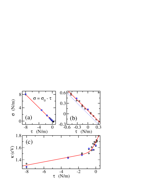
Figure 1: (a) Dependence of the fluctuation tension, $\sigma,$ of graphene with the mechanical tension $\tau$. Symbols are derived from $N\tau T$ simulations at 300 K with $N=960$ (black circles) and $N=8400$ (blue squares). The full line is a linear fit; (b) Zoom of $\sigma$ for small mechanical tensions. The dotted line is the harmonic expectation $\sigma=-\tau$; (c) Results for the bending constant $\kappa$. The full line shows a least-squares fit of the simulation data.

III.2 Finite-size effects

Finite-size effects are significant in graphene simulations.(Los et al., 2016) The amplitude of the out-of-plane fluctuations,

$$\left\langle h^{2}\right\rangle=\frac{1}{N}\sum_{j=1}^{N}\left\langle h_{j}^{2}\right\rangle\>,$$ (9)

is a function of $\sigma$ and $\kappa$, as these variables define the long-wave limit of the ZA modes. Let us study the finite-size error of the average $\left\langle h^{2}\right\rangle_{N_{0}}$ obtained in a $N_{0}\tau T$ simulation. The $\mathbf{k}_{ln}$-grid in Eq. (4) for the size $N_{0}$ is made up of elementary rectangles $R_{i}$. Let $R_{0}$ be the rectangle having the $\Gamma$ point at one vertex. The values of $(l,n)$ for the vertices of $R_{0}$ are (0,0), (0,1), (1,0), and (1,1), with (0,0) as the $\Gamma$-point. Let us now consider successively larger cells defined with $N=N_{0}n_{k}^{2}$, where $n_{k}=$$1,2,\ldots$ is an integer scaling factor. Geometry in $\mathbf{k}$-space dictates that the larger the cell size, the denser the $\mathbf{k}$-grid. The number of $\mathbf{k}$-points in the elementary area $R_{0}$ increases as $(n_{k}+1)^{2}$, i.e., it grows as $2^{2},3^{2},4^{2},\ldots$ for $N$ increasing as $N_{0},2^{2}N_{0},3^{2}N_{0},\ldots$. The finite-size correction for $\left\langle h^{2}\right\rangle_{N_{0}}$ is based on a discrete sum in reciprocal space. The sum is over the $(n_{k}+1)^{2}$ $\mathbf{k}$-points in $R_{0}$

$$C_{N}=\frac{4}{N}\sum_{l=0}^{n_{k}}\sum_{n=0}^{n_{k}}{}^{{}^{\prime}}\alpha_{ln}\bar{H}_{ln}^{2}\>.$$ (10)

The prime indicates that the $\Gamma$-point ($l=n=0$) is excluded from the sum. The multiplicative factor is the number of elementary areas, $R_{0}$, in the Brillouin zone. It is equal to the multiplicity of a general position in $k$-space, i.e., 4 (6) for a 2D rectangular (hexagonal) unit cell. The amplitudes $\bar{H}_{ln}^{2}$ are calculated by Eq. (5) with the analytic long-wave approximation $\rho\omega_{ln}^{2}=\sigma k_{ln}^{2}+\kappa k_{ln}^{4}$. The weight factors $\alpha_{ln}$ are unity except for those $\mathbf{k}_{ln}$ points at the vertices ($\alpha_{ln}=1/4)$ and sides ($\alpha_{ln}=1/2)$ of $R_{0}$. The finite-size correction to the average $\left\langle h^{2}\right\rangle_{N_{0}}$ is then

$$\left\langle h^{2}\right\rangle_{N}\approx\left\langle h^{2}\right\rangle_{N_{0}}+C_{N}-C_{N_{0}}\>.$$ (11)

To check the reliability of this analytical model, we have compared results for $\left\langle h^{2}\right\rangle_{N}$ derived from $N_{0}=24$ using Eq. (11), with those obtained directly from simulations with $N$ atoms. Results for $\left\langle h^{2}\right\rangle$ at 300 K and $\tau=0$ with $N$ varying between 24 and 33600 atoms are displayed in Fig. 2a as open circles. The finite-size correction for $N_{0}=24$ is shown as a broken line. The agreement with the simulation data is very good. Note that the average $\left\langle h^{2}\right\rangle=6\times 10^{-5}$ nm² for $N=24$ increases by two orders of magnitude for $N=33600$. The dispersion law $\rho\omega^{2}=\sigma k^{2}+\kappa k^{4}$ correctly predicts the finite-size effect in $h^{2}$. The values of $\sigma$ and $\kappa$ at $\tau=0$ are 0.094 N/m and 1.7 eV (see Fig. 1). The finite-size correction obtained with $N_{0}=960$ is nearly indistinguishable from that with $N_{0}=24$, an indication of the consistency of our approach. The dispersion law, $\omega(k)$, implies that $\left\langle h^{2}\right\rangle$ increases with the size of the sample as $\ln N$.(Ramírez et al., 2016)

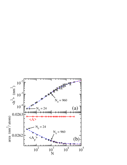
Figure 2: $(a)$ Amplitude of the ZA modes as a function of the number of atoms in the simulation cell. Symbols are $N\tau T$ simulation results for $\left\langle h^{2}\right\rangle$ at 300 K and $\tau=0$. Broken and dotted lines are finite-size corrections for $N_{0}=24$ and $960$ atoms, respectively. The two lines are nearly indistinguishable. $(b)$ Circles are the simulation results for the projected area $\left\langle A_{p}\right\rangle$. The broken and dotted lines are finite-size extrapolations of the simulations with $N_{0}=24$ and $960$ atoms, respectively. Squares display the real area $\left\langle A\right\rangle$ from simulations with $N=24$. The continuous line is a guide to the eye.

A similar scheme applies to the size correction of $\left\langle A_{p}\right\rangle_{N_{0}}$. Differential elements of the real and projected areas are related by the surface metric as(Safran, 1994)

$$dA=(1+h_{x}^{2}+h_{y}^{2})^{1/2}dA_{p}\approx\left(1+\frac{h_{x}^{2}+h_{y}^{2}}{2}\right)dA_{p}\>,$$ (12)

where $h_{x}$ ($h_{y}$) denotes the partial derivative of the height $h$ with respect to $x$ ($y$), and the r.h.s. is a first-order approximation when deviations from planarity are small. By integration of the r.h.s and after Fourier transform one derives(Safran, 1994)

$$S_{N}=\frac{4}{N}\sum_{l=0}^{n_{k}}\sum_{n=0}^{n_{k}}{}^{{}^{\prime}}\alpha_{ln}\frac{1}{2}k_{ln}^{2}\bar{H}_{ln}^{2}.$$ (13)

The sum $S_{N}$ in reciprocal space provides the finite-size correction to the projected area $\left\langle A_{p}\right\rangle_{N_{0}}$ as

$$\left\langle A_{p}\right\rangle_{N}\approx\left\langle A_{p}\right\rangle_{N_{0}}+S_{N}-S_{N_{0}}\>.$$ (14)

Simulation results for the projected area $\left\langle A_{p}\right\rangle$ are presented in Fig. 2b as open circles. Size effects are significant. $\left\langle A_{p}\right\rangle$ decreases with increasing $N$, and converges to a finite area per atom for $N\rightarrow\infty$. This behavior is in good agreement to previous Monte Carlo (MC) simulations with the LCBOPII model.(Los et al., 2016) The finite-size correction for $N_{0}=24$ using Eq. (14) is shown as a broken line. A remarkable agreement to the simulation data is found. The correction with $N_{0}=960$ is nearly indistinguishable from that with $N_{0}=24.$

Simulation results of the real area $\left\langle A\right\rangle$ with $N=24$ are shown in Fig. 2b. $A$ is calculated by triangulation of the surface, with C atoms and hexagon centers as vertices of the triangles. Hexagon centers are located at the average position of their six vertices. The area $\left\langle A\right\rangle$, in contrast to $\left\langle A_{p}\right\rangle$, displays a small finite-size error, not visible at the scale of Fig. 2b. For $N=24$, the relative finite-size error in $\left\langle A\right\rangle$ amounts to $2\times 10^{-3}$ %, while that of $\left\langle A_{p}\right\rangle$ is two orders of magnitude larger, $0.3$ %. A larger size, $N\sim 4\times 10^{4}$, is needed to reduce the finite-size error of $\left\langle A_{p}\right\rangle$ to the small error achieved for $\left\langle A\right\rangle$ with $N=24$. Note that our finite-size correction considers only the acoustic ZA mode. The obtained results imply that the rest of vibrational modes (namely the in-plane and optical out-of-plane (ZO) modes of the layer) display a comparatively small size effect.

The difference between $A$ and $A_{p}$ for a continuous membrane in the $N\rightarrow\infty$ limit can be calculated by integration and Fourier transform of the r.h.s. of Eq. (12).(Safran, 1994; Chacón et al., 2015) With the ZA dispersion law, $\rho\omega^{2}=\sigma k^{2}+\kappa k^{4}$, one gets

$$A=A_{p}\left(1+\frac{k_{B}T}{4\pi}\int_{0}^{k_{max}}dk\frac{k}{\sigma+\kappa k^{2}}\right)=$$

$$=A_{p}\left[1+\frac{k_{B}T}{8\pi\kappa}\ln\left(1+\frac{2\pi\kappa}{\sigma A_{p}}\right)\right]\>,$$ (15)

with $k_{max}=\left(2\pi/A_{p}\right)^{1/2}$. A quadratic term $\sigma k^{2}$ in $\rho\omega^{2}$ is a sufficient condition for the convergence of the integral.

III.3 Elastic moduli

We focus now on the elastic moduli of graphene. First, the finite-size correction $\left\langle A_{p}\right\rangle_{N}$ is derived with $N_{0}=24$ at mechanical tensions $\tau$ in the range $-4$ to $0.05$ N/m, using the values of $\sigma$ and $\kappa$ shown in Fig. 1. For each tension $\tau$ and size $N$, $\left\langle A_{p}\right\rangle_{N}$ is then obtained at two close tensions $\tau\pm$0.016 N/m, in order to calculate numerically the derivative $\partial\left\langle A_{p}\right\rangle_{N}/\partial\tau$. The bulk modulus $B_{p}$ for size $N$ is then obtained as

$$B_{p}=-\left\langle A_{p}\right\rangle_{N}\frac{\partial\tau}{\partial\left\langle A_{p}\right\rangle_{N}}\>.$$ (16)

The values of $B_{p}$ for the sizes $24n_{k}^{2}$, with $n_{k}=6$ ($N=864$) and $n_{k}=7$ ($N=1176$ ) are plotted in Fig. 3a as dotted and full lines, respectively. For comparison, open circles display $B_{p}$ from $N\tau T$ simulation with $N=960$ atoms, as derived from the fluctuation formula(Herrero, 2008)

$$B_{p}=\frac{k_{B}T\left\langle A_{p}\right\rangle}{N\left(\left\langle A_{p}^{2}\right\rangle-\left\langle A_{p}\right\rangle^{2}\right)}\>.$$ (17)

It is remarkable the agreement between the values of $B_{p}$ from the simulations with $N=960$ atoms and from the finite-size extrapolation with $N_{0}=24$. This agreement is more demanding than that of $\left\langle h^{2}\right\rangle$ and $\left\langle A_{p}\right\rangle$ in Fig. 2, because of the wide range of studied mechanical tensions.

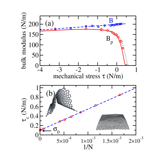
Figure 3: $(a)$ Bulk moduli of graphene at 300 K as a function of the mechanical tension $\tau$. $B$ and $B_{p}$ are defined with respect to the real and projected areas, $A$ and $A_{p},$ respectively. Circles are simulation results of $B_{p}$ for $N=960$. The dotted and continuous lines are extrapolations of $B_{p}$ for $N=864$ and $N=1176$ atoms, respectively. Both lines were derived by finite-size correction of simulations with $N_{0}=24$ atoms. Squares are simulation results of $B$ for $N=24$ atoms. The broken line is a linear fit. $(b)$ Critical mechanical tension as a function of the number of atoms. Results derived by finite-size correction of simulations with $N_{0}=24$ atoms. Typical atomic structures with $N=960$ are shown below (planar layer) and above (wrinkled layer) the critical tension.

The bulk modulus, $B$, calculated from the fluctuation of the real area, $\left\langle A\right\rangle$, in simulations with $N=24$ is shown as open squares in Fig. 3. The finite-size effect in $B$ is negligible at the scale of Fig. 3a, in line with the negligible finite-size effect in the real area $\left\langle A\right\rangle$ (see Fib. 2b). $B$ and $B_{p}$ behave quite differently. The anharmonicity causes a finite derivative of $B$ with respect to $\tau$, $B^{\prime}\sim 7.$ $B_{p}$ is close to $B$ at the largest studied negative tensions, when out-of-plane fluctuations are small, but $B_{p}$ becomes much smaller than $B$ as $\tau$ increases. At a critical compressive tension, $\tau_{c}>0,$ the bulk modulus $B_{p}$ vanishes. $\tau_{c}$ represents the stability limit for a planar layer before the stable configuration becomes wrinkled. $\tau_{c}$ displays a strong size effect that is shown in Fig. 3b. The critical mechanical tension, $\tau_{c},$ decreases with the number of atoms as $N^{-1}$. In the thermodynamic limit we get $\tau_{c}=\sigma_{0}$, i.e., a planar layer is able to sustain a compressive tension of about $\tau_{c}\sim 0.1$ N/m before becoming wrinkled. The structural plots in Fig. 3b shows that wrinkles are generated along a preferential direction.

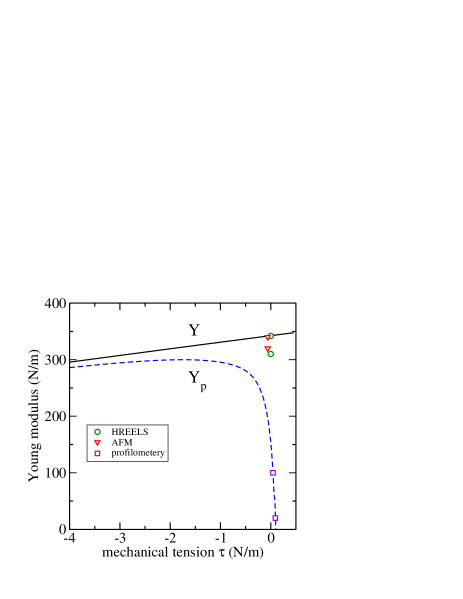
Figure 4: The Young moduli, $Y$ and $Y_{p},$ are displayed at 300 K as a function of the mechanical tension $\tau$. $Y$ and $Y_{p}$ are defined with respect to the real and projected areas, $A$ and $A_{p},$ respectively. $Y_{p}$ was derived by finite-size correction of the simulation with $N_{0}=24$ atoms. $Y$ displays a very small size effect and it was derived by a least-squares fit of simulations with $N=24$ atoms. The Poisson ratio is $\nu=0.15$. Symbols are experimental values of the Young modulus of graphene as measured by HREELS,(Politano and Chiarello, 2015) AFM, (Lee et al., 2008, 2013; Lopez-Polin et al., 2015) and interferometric profilometery.(Nicholl et al., 2015)

The Young modulus, $Y$, of a 2D layer is related to the bulk modulus by $Y=2B(1-\nu)$, where $\nu$ is the Poisson ratio. We have calculated $\nu=0.15$ for the employed LCBOPII model in the classical $T\rightarrow 0$ limit. Using this value, the Young moduli, $Y$ and $Y_{p}$, of graphene have been plotted in Fig. 4 as a function of $\tau$. $Y_{p}$ was derived in the thermodynamic limit ($N\rightarrow\infty$) by applying the finite-size correction to simulations with $N_{0}=24$. $Y$ has a small size effect and it was derived by a least-squares fit of simulations with $N=24$ atoms. The Young modulus $Y$, related to the real area $A$, shows a monotonic dependence with $\tau$. For $\tau=0$ we find $Y=339$ N/m. On the other side, $Y_{p}$ displays a maximum ($297$ N/m) at $\tau=-1.7$ N/m, decreases rapidly for $\tau\gtrsim-1$ N/m and vanishes at the critical tension $\tau_{c}=0.1$ N/m.

Experimental HREELS results of the Young modulus of both planar and corrugated graphene supported on a variety of metal substrates are displayed in Fig. 4 as open circles.(Politano and Chiarello, 2015) HREELS provides in-plane phonon dispersion curves. The elastic constants derived from the sound velocities of the acoustic in-plane branches are a property related to the real area of the layer that should correspond to the observable $Y$. In fact, we find good agreement between the HREELS results and our simulation results for $Y$. Results from AFM indentation experiments, shown as triangles in Fig. 4, also agree with our simulation results for $Y$.(Lee et al., 2008, 2013; Lopez-Polin et al., 2015) The lack of correlation between the elastic modulus and the mechanical tension, reported in the experiments of Ref. Lopez-Polin et al., 2015, is in line with the weak dependence of the simulation results of $Y$ on the value of $\tau$. However, elastic constants from interferometric profilometery are derived by fitting the experimental data to an average surface.(Nicholl et al., 2015) These elastic constants, plotted as squares in Fig. 4, should correspond to the observable $Y_{p}$. The two interferometric profilometery results are displayed at mechanical tensions of 0.04 and 0.09 N/m. The tension of the graphene layer depends on the sample processing by factors that can not be controlled experimentally. Thus the previous tensions have been chosen to fit the experimental data to our $Y_{p}$ curve.

IV Summary

We have analyzed the long-wave limit of the acoustic transverse fluctuations of graphene at 300 K. A finite-size correction for the out-out-plane amplitude, $h^{2}$, the projected area, $A_{p}$, and the bulk modulus, $B_{p}$, has been based on the dispersion relation, $\rho\omega^{2}=\sigma k^{2}+\kappa k^{4}$. The size correction has small computational cost, displays excellent agreement to simulations with larger cells, and strongly supports the validity of the acoustic dispersion law in graphene. The fluctuation tension, $\sigma$, depends on the external mechanical tension, $\tau$, by an anharmonic relation, $\sigma=\sigma_{0}-\tau$. At 300 K we find $\sigma_{0}\sim 0.1$ N/m. The finite value of $\sigma_{0}$ has a large influence in the amplitude of the out-of-plane fluctuations and in the mechanical stability of the crystalline membrane against wrinkling. The Young modulus, $Y_{p}$, related to the projected area varies between 0 and $\sim 300$ N/m depending upon the mechanical tension sustained by the layer. However, the Young modulus, $Y$, related to the real area, amounts to $340$ N/m in the absence of external mechanical tension, and decreases to $\sim 300$ N/m for large tensile stresses of -4 N/m. The existence of two different observables, $Y$ and $Y_{p}$, provides a reliable explanation for the experimental values of the Young modulus of graphene as measured by HREELS, AFM, and interferometric profilometery.