Optimal quantum tomography

Abstract

The present short review article illustrates the latest theoretical developments on quantum tomography, regarding general optimization methods for both data-processing and setup. The basic theoretical tool is the informationally complete measurement. The optimization theory for the setup is based on the new theoretical approach of quantum combs.

I Introduction

Fine calibration of apparatuses is the basis of any precise experiment, and the quest for precision and reliability is relentlessly increasing with the strict requirements of the new photonics, nanotechnology, and the new world of quantum information. The latter, in particular, depends crucially on the reliability of processes, sources and detectors, and on precise knowledge of all sources of noise, e.g. for error correction.

But what does it mean to calibrate a quantum device? It is really a much harder task than calibrating a classical “scale”. For example, for calibrating a photo-counter, we don’t have standard sources with precise numbers of photons—the equivalent of the “standard weights” for the scale. Even worst, we never know for sure that all photons have been actually absorbed by the detector. The practical problem is then to perform a kind of quantum calibration to determine in a purely experimental manner (by relying on some well established measuring instruments) the quantum description of our device, without the need of a detailed theoretical knowledge of its inner functioning—being it a measuring apparatus, a quantum channel, a quantum gate, or a source of quantum states.

And here it comes the powerful technique of quantum tomography. Originally invented for determining the quantum state of radiation (for recent reviews see the book [1] and e. g. Refs. [2, 3], it soon became the universal measuring technique by which one can determine any ensemble average and measure the fine details of any quantum operation, channel, or measuring instruments—objects that before were just theoretical tools (for history and references see next section).

In the present short review article we will illustrate our latest theoretical developments on quantum tomography, consisting in a first systematic theoretical approach to optimization of both data-processing and setup. Therefore, apart from the historical excursus of the next section, where we mention the relevant contributions from other authors, the body of the paper is focus only on our theoretical work.

The basic tool of the theoretical approach is the informationally complete measurement [4] (see Refs. [5, 6] for applications in the present context)—corresponding to the mathematical theory of operator bases. The optimization of data-processing [7] relies on the fact that as an operator basis the informationally complete measurement is typically linearly dependent, allowing different expansion coefficients, which can be then optimized, according to specific criteria. The optimization theory for the setup [8], on the other hand, needs the new theory of quantum combs and quantum testers [9], novel powerful notions in quantum mechanics, which generalize those of quantum channel and of POVM (positive-operator-valued measure). These will be briefly reviewed in the section before conclusions. As the reader will see, the theoretical framework is sufficiently general and mature for a concrete optimization in the lab, i.e. accounting for realistic bounded resources, and this will be the direction of future development of the field.

II Historical excursus

Quantum tomography is a relatively recent discipline. However, the possibility of “measuring the quantum state” has puzzled physicists in the last half century, since the earlier theoretical studies of Fano [10] (see also Pauli in Ref. [11]). That more than two observables—actually a complete set of them, a so-called quorum of observables [12, 13]—are needed for a complete determination of the density matrix was immediately clear [10]. However, in those years it was hard to devise concretely measurable observables other than position, momentum and energy (Royer pointed out that instead of measuring varying observables one can vary the state itself in a controlled way, and measure e. g. just its energy [16]). For this reason, the fundamental problem of determining the quantum state remained at the level of mere speculation for many years. The issue finally entered the realm of experiments only less than twenty years ago, after the pioneering experiments by Raymer’s group [17], in the domain of quantum optics. Why quantum optics? Because in quantum optics, differently particle physics, there is the unique opportunity of measuring all possible linear combinations of position and momentum of a harmonic oscillator, representing a single mode of the electromagnetic field. Such measurement can be achieved by means of a balanced homodyne detector, which measures the quadrature $X_{\phi}=\frac{1}{2}\left(a^{\dagger}e^{i\phi}+ae^{-i\phi}\right)$ of a field mode at any desired phase $\phi$ with respect to the local oscillator (LO) [as usual $a$ denotes the annihilator of the field mode]. The first technique to reconstruct the density matrix from homodyne measurements—so called homodyne tomography—originated from the observation by Vogel and Risken [18] that the collection of probability distributions $\{p(x,\phi)\}$ for $\phi\in[0,\pi)$ is just the Radon transform—i.e. the tomography—of the Wigner function $W$. Therefore, by a Radon transform inversion, one can obtain $W$, and from $W$ the matrix elements of the density operator $\rho$. This first method, however, works fine only for high number of photons or for almost classical states, whereas in the truly quantum regime is affected by the smoothing needed for the Radon transform inversion. The main physical tool, however—i.e. using homodyning—was a perfectly good idea: one just needed to process the experimental data properly.

In Ref.[19] the first exact technique was given for measuring experimentally the matrix elements of $\rho$ in the photon-number representation, by just averaging functions of homodyne data. After that, the method was further simplified [20], and the feasibility for nonunit quantum efficiency $\eta<1$ at detectors—above some bounds—was established. Further improvements in the numerical algorithms made the method so simple and fast that it could be implemented easily on small PCs, and the method became quite popular in the laboratories (for the earlier progresses and improvements the reader can see the old review [21]). In the meanwhile there has been an explosion of interest on the subject of measuring quantum states, with hundreds of papers, both theoretical and experimental. The exact homodyne method has been implemented experimentally to measure the photon statistics of a semiconductor laser [22], and the density matrix of a squeezed vacuum[23]. The success of optical homodyne tomography has then stimulated the development of state reconstruction procedures for atomic beams [24], the experimental determination of the vibrational state of a molecule [25], of an ensemble of helium atoms [26], and of a single ion in a Paul trap [27], and different state reconstruction methods have been proposed (for an extensive list of references of these first pioneering years, see e.g. Ref. [28]).

Later the method of quantum homodyne tomography has been generalized to the estimation of an arbitrary observable of the field [29], with any number of modes [30], and, to arbitrary quantum systems via group theory [31, 32, 33], and with a general method for unbiasing noise [31, 32]. Eventually, it was recognized that the general data-processing is just an application of the theory of operator expansions[34, 35], which lead to identify quantum tomography as an informationally complete measurement [36]—a generalization of the concept of quorum of observables [12, 13].

State reconstruction was extended to the case where an incomplete measurement is performed. In this the reconstruction of the full density matrix of the system is actually impossible, and one can only estimate the state that best fits the measured data applying the Jaynes’s maximum entropy principle (MaxEnt) [14]. When one has some non-trivial prior information the fit can be improved by minimizing the Kullback-Leibler distance from a given state which represents this a priori information [15].

At the same time, in alternative to the averaging data-processing strategy of the original method [19], it was recognized in Refs. [37, 38] the possibility of implementing a maximum likelihood strategy for reconstructing the diagonal of the density matrix, and later for the full matrix [39]. An advantage of the maximum likelihood strategy is that the density matrix is constrained to be positive, whereas positivity can be violated in the fluctuations of the averaging strategy. In addition, the maximum likelihood often allows to reduce dramatically the number of experimental data for achieving the same statistical error, at the expense of a bias, which is however negligible in many cases of practical interest. However, there is a drawback: this is the need of estimating the full density matrix (the strategy is essentially a maximization of the joint probability of the full data-set over all possible density matrices, or Bayesian variations of such maximization accounting for prior knowledge[40]). This, on one side requires a cutoff of the dimension of the Hilbert space when infinite (such as for the harmonic oscillator, as in homodyne tomography), thus introducing the mentioned bias; on the other side it has computational and memory complexities which increase exponentially with the number of systems for a joint tomography on multiple systems. On the contrary, the averaging strategy for any desired expectation value needs just to average a single function of the experimental outcome, without needing the full matrix, and this includes as a special case the evaluation of single matrix element itself, whence without necessitating a dimensional cutoff.

Contemporary to this preliminary evolution of data-processing methods, there has been also a parallel evolution in the tomographic setup design. It was realized that it is possible not only states, but also channels [41, 42]—the so-called (standard quantum) process tomography (SQPT)—based on the idea of tomographing the outputs of a channel corresponding to a set of input states making an operator basis for all density matrices. However, soon later it was recognized (first for the diagonal matrix elements in the number basis of an optical process [43], then in general for any channel [44, 45] that the same process tomography can be actually achieved using just a single input state entangled (with maximal Schmidt number) with an ancilla—the so-called ancilla-assisted process tomography (AAPT)—exploiting the “quantum parallelism” of the entangled input state which plays the role of a “superposition of all possible input states”. This can have a great experimental advantage when the basis of states is not easily achievable experimentally, whereas the entangled state is, as in the case of homodyne tomography where it is easy to achieve such entangled state from parametric down-conversion of vacuum, whereas it is hard to achieve photon-number states (see however, Ref. [46], where a set of random coherent states have been proposed as a basis). As later proved in Ref. [47], and experimentally verified in Refs. [48], almost any joint system-ancilla state can be exploited for AAPT. On the other hand, the same AAPT has been extended to quantum operations and to measuring apparatus [49, 50] (former theoretical proposals for calibration of detectors were published without ancilla [52, 53], and even ancilla-assisted [54]). Later, by another kind of quantum parallelism, it was recognized that one can also estimate the ensemble average of all operators of a quantum system by measuring only one fixed ”universal” entangled observable on an extended Hilbert space [55]—a truly universal observable. At this point the tomographic method had reached the stage in which a single fixed apparatus (single preparation of the input and single observable at the output) is needed, in principle reducing enormously the experimental complexity for joint tomography on many systems (complexity 1 versus exponential complexity).

After the first experimental SQPT by NMR [56], AAPT was experimentally proved in Refs. [57, 48], for photon polarization qubit quantum operations, exploiting spontaneous parametric downconversion in a non linear crystal as a source of entangled states.

As in the case of state tomography, the freedom in the choice of the experimental configuration poses the natural question of what is the optimal setup for a given figure of merit. In Ref. [58] the issue of minimizing the number of different experimental configurations needed for process tomography was raised again, and a the so-called Direct Characterization of Quantum Dynamics (DCQD) setup was introduced for qubits, later generalized to arbitrary finite dimensional systems [59]. The proposed protocol starts from the expression of the Choi-Jamiołkowski operator (also called $\chi$-matrix) $\mathscr{C}(\rho)=\sum_{mn}\chi_{mn}A_{m}\rho A_{n}^{\dagger}$ of the quantum channel $\mathscr{C}$ operating on the inputs state $\rho$, choosing for the basis $\{A_{m}\}$ the shift-and-multiply group elements, and then uses techniques from error detection for the estimation of parameters $\chi_{mn}$ from estimated error probabilities. The DCQD approach is interesting because of the interpretation of Process Tomography in terms of error detection, however, it does not provide any optimality argument in terms of number of experimental configurations, apart from a vague resource analysis [60]. A similar scheme was introduced in Ref. [61], where the authors provide a method for process tomography that allows to separately reconstruct the Choi operator matrix elements in a fixed basis based by Haar-distributed input state sampling. The authors exploit spherical $2$-designs [62] in order to discretize the required averaging over the group $\mathbb{SU}(d)$.

In more recent years some experiments in the continuous-variable domain were performed both for process tomography [63] and for measurement calibration [64], however both experiments exploited the SQPT technique, while no AAPT experiments with continuous variable systems have been reported so far. Many tomographic experiments on different kinds of quantum systems have been performed, like atoms in optical lattices [65], cold ions in Paul traps [66], NMR probed molecules [67], solid state qubits [68], and quantum optic cavity modes interacting with atoms [69].

In the last decade the interest in quantum tomography grew very fast with the increasing number of applications in the hot field of quantum information, allowing testing the accuracy of state-preparation and calibration of quantum gates and measuring apparatuses. One should realize that the whole technology of quantum information crucially depends on the reliability of processes, source and detectors, and on precise knowledge of sources of noise and errors. For example, all error correction techniques are based on the knowledge of the noise model, which is a prerequisite for an effective design of correcting codes [70, 71, 72], and Quantum Process Tomography allows a reliable reconstruction of the noise and its decoherence free subspaces without recurring to prior assumptions on the noisy channels [73]. The increasingly high confidence in the tomographic technique, with the largest imaginable flexibility of data-processing, and expanding outside the optical domain in the whole physical domain, grew the appetite of experimentalists and theoreticians posing increasingly challenging problems. The relevant issues were now to establish the optimal tomographic setups and data-processing, and to minimize the physical resources, handling increasingly large numbers of quantum system jointly. Regarding this last point, a relevant issue is the exponentially increasing dimension of the Choi operator of the quantum process versus the number of systems involved, and methods for safely neglecting irrelevant parameters in multiple qubit noise model reconstruction have been introduced [74] based on assumptions of qubit noise independence and Markovianity. In Ref. [75], methods to tackle the case of sparse Choi matrices are shown, expressing the minimum $\ell_{1}$-norm distance criterion in terms of a standard convex optimization problem. On the problem of optimizing data-processing, on the other hand, upper bounds on minimal Hilbert-Schmidt distance between the estimated and the actual Choi-Jamiołkowski state has been derived[76] exploiting spherical $2$-designs. It can be shown that minimizing such a distance is equivalent to the minimizing the statistical error in the estimation of any ensemble average evolved by the channel. On the other hand, a systematic way of posing the problem of optimizing the data-processing is to fix a cost-function (depending on the purpose of the tomographic reconstruction), and minimize the average cost—the canonical procedure in quantum estimation theory [77].

The optimal data-processing for any measurement (in finite-dimensions) for estimating the expectation of any observable with minimum error was derived in Ref. [7]. On the other hand, in regards of the optimal setups, an approach based on the theory of quantum combs and quantum testers [9, 78] have been introduced, that allowed to determine the optimal schemes (minimizing the statistical error in estimating expectation values) for all of the three kinds of tomography: state, process, and measurement [8] (quantum combs and quantum testers generalize the notion of channels and POVM’s). The optimal setups use up to three ancillas, and need only a single input state (with bipartite entanglement only) and the measurement of a Bell basis, with a variable local unitary shifts of the ancillas. Exploiting the same approach incomplete process tomography has been addressed in Ref. [79] using “process entropy”, the analogous of the max-entropy method [14] for process tomography.

III methodology

In the following we will treat linear operators $X$ from $\mathcal{H}_{0}$ to $\mathcal{H}_{1}$ as elements of a vector space, and the following formula is very useful

$$|X\rangle\!\rangle:=\sum_{m=0}^{d_{1}-1}\sum_{n=0}^{d_{0}-1}X_{mn}|m\rangle_{1}|n\rangle_{0}.$$ (1)

In Eq. (1) $d_{i}$ denotes the dimension of the Hilbert space $\mathcal{H}_{i}$, $\{|n\rangle_{i}\}$ are orthonormal bases for for $\mathcal{H}_{i}$ $i=1,2$, and $X_{mn}$ are the matrix elements of $X$ on the same orthonormal basis.

A general mathematical framework for quantum tomography was introduced in Refs. [34, 35], based on spanning sets of observables called quorums. In we will review the more general approach based on informationally complete POVMs [5, 6]. A POVM is a set of positive operators $\{P_{l}\}$ that add up to the identity. The method is based on operator expansions, and we will show how expanding operators on a POVM can be used to reconstruct their expectation values on the state of the measured system. The aim of a tomographic reconstruction is to obtain the ensemble expectation of an operator $X$ by averaging some function $f_{l}[X]$ depending on the outcome of a suitable POVM $\{P_{l}\}$. We require the procedure to be unbiased, namely the reconstruction must be as follows

$$\langle X\rangle_{\rho}=\sum_{l}f_{l}[X]p(l|\rho),\quad p(l|\rho):=\mathrm{Tr}[\rho P_{l}].$$ (2)

Whatever notion of convergence one uses, the requirement for unbiasedeness implies—by the polarization identity—that the following expansion for the operator $X$ holds

$$X=\sum_{l}f_{l}[X]P_{l},$$ (3)

where the sum can be replaced by an integral in the case of continuous outcome set (the expansion clearly is defined for weakly convergent sum, meaning that Eq. (2) holds for all states $\rho$). The general reconstruction method consists in finding expansion coefficients $f_{l}[X]$, and then averaging them over the outcomes $l$. In this way one can define the expansion for general bounded operators $X$. Further extensions of the definition in Eq. (3) to unbounded operators can be obtained requiring the convergence of Eq. (2) for states $\rho$ in a dense set $\mathcal{S}$ (e. g. finite energy states). A particularly simple case is that of operators on finite dimensional Hilbert spaces, or for Hilbert-Schmidt operators in infinite dimensional spaces, since in these cases the space of operators is a Hilbert space itself, equipped with the Hilbert-Schmidt product $\langle\!\langle A|B\rangle\!\rangle:=\mathrm{Tr}[A^{\dagger}B]$, and convergence of Eq. (3) can be defined in the Hilbert-Schmidt norm $\left|\!\left|X\right|\!\right|:=\sqrt{\langle\!\langle X|X\rangle\!\rangle}$.

Clearly, the use of the formula in Eq. (2) for estimation of $\langle X\rangle_{\rho}$ (for all $\rho\in\mathcal{S}$ and for all $X$ such that $\mathrm{Tr}[\rho X]$ is defined on $\mathcal{S}$) is possible iff $\{P_{l}\}$ is a complete set in the space of linear operators. Such a POVM is called informationally complete [4]. For the sake of simplicity, in the following we will restrict attention to the case of Hilbert-Schmidt operators $X$. Eq. (3) defines a linear map $\Lambda$ from the vector space of coefficients ${\bf f}:=(f_{l})$ to linear operators as follows

$$\Lambda{\bf f}=\sum_{l}f_{l}P_{l},$$ (4)

whose domain contains all the vectors $\bf f$ such that the sum in Eq. (4) converges (either in Hilbert-Schmidt norm or weakly). As we mentioned before, a reconstruction strategy requires a choice of coefficients ${\bf f}[X]$ for any operator $X$, such that $\Lambda{\bf f}[X]=X$. In algebraic terms, the choice corresponds to a generalized inverse $\Gamma$ of $\Lambda$ defined by $\Lambda\Gamma\Lambda=\Lambda$, so that ${\bf f}[X]=\Gamma(X)$ [80]. When the set $\{P_{l}\}$ is not linearly independent the inverse $\Gamma$ is not unique, and this implies that one can choose the coefficients ${\bf f}[X]$ according to some optimality criterion, as we will explain in Sec. VIII. Notice that by linearity, any inverse $\Gamma$ provides a dual spanning set $\{Q_{l}\}$ whose matrix elements are $(Q_{l})^{*}_{mn}:=f_{l}[E_{mn}]$, with $E_{mn}:=|m\rangle\langle n|$, namely $f_{l}[X]=\mathrm{Tr}[Q^{\dagger}_{l}X]$.

As we will see in the next sections, for finite dimensional systems the theory of generalized inverses is sufficient for classifying all possible expansions and consequently deriving the optimal coefficients ${\bf f}[X]$ for a fixed POVM $\{P_{l}\}$, [7, 84]. On the other hand, the full classification of inverses $\Gamma$ and consequent optimization is a still unsolved problem for infinite dimensional systems, for which alternative approaches are useful [83].

III-A Frames

In this subsection we will review the relevant results in the theory of frames on Hilbert spaces, which is useful for dealing with POVMs on infinite dimensional systems [83] where a classification of all inverses $\Gamma$ is still lacking. The method for evaluating possible inverses provided in Refs. [34, 35] is an orthogonalization algorithm—similar to the customary Gram-Schmidt method—based on the assumption that the POVM is a frame [81] in the Hilbert space of Hilbert-Schmidt operators, namely that the two following inequalities hold

$$a\left|\!\left|X\right|\!\right|^{2}\leq\sum_{l}|\langle\!\langle P_{l}|X\rangle\!\rangle|^{2}\leq b\left|\!\left|X\right|\!\right|^{2}.$$ (5)

Equivalently, $\{P_{l}\}$ is a frame iff its frame operator

$$F:=\sum_{l}|P_{l}\rangle\!\rangle\langle\!\langle P_{l}|,$$ (6)

is bounded and invertible with bounded inverse. The theory of frames provides a (partial) classification of inverses $\Gamma$ in terms of dual frames for $\{P_{l}\}$, namely those frames $Q_{l}$ such that the following identity holds in the vector space of operators

$$\sum_{l}|P_{l}\rangle\!\rangle\langle\!\langle Q_{l}|=I.$$ (7)

While the orthogonalization method is effective in providing adequate coefficients ${\bf f}[X]$ for the purpose of evaluating the expectation value of operators $X$, it maybe inefficient in minimizing the statistical errors, since the orthogonalization would be equivalent to discard experimental data. On the other hand, using the method of alternate duals of a frame allows one to use all experimental data in the most efficient way, according to any chosen criterion, such as minimize the statistical error. We will now show how the method works,

The canonical dual frame is defined as

$$|D_{l}\rangle\!\rangle:=F^{-1}|P_{l}\rangle\!\rangle,$$ (8)

and it trivially satisfy Eq. (7). All alternate dual frames of a fixed frame $\{P_{l}\}$ are classified in Ref. [82], and they are given by the following expression

$$Q_{l}=D_{l}+Y_{l}-\sum_{j}\langle\!\langle D_{l}|P_{j}\rangle\!\rangle Y_{j},$$ (9)

where $Y_{l}$ is arbitrary, provided that the sum $\sum_{j}\langle\!\langle D_{l}|P_{j}\rangle\!\rangle Y_{j}$ converges. It is clear from the definition in Eq. (7) that any dual frame $\{Q_{l}\}$ corresponds to an inverse $\Gamma$, via the identification $\Gamma(X)={\bf f}[X]$, with the coefficients given by

$$f_{l}[X]:=\langle\!\langle Q_{l}|X\rangle\!\rangle.$$ (10)

For finite dimensions also the converse is true, namely any inverse $\Gamma$ provides a dual set $\{Q_{l}\}$ which is a frame. However, in the infinite dimensional case it is not guaranteed that all the dual sets corresponding to inverses $\Gamma$ are frames themselves.

The results in this subsection can be generalized to frames for bounded operators (for the theory of frames for Banach spaces, see Ref. [85]) by weakening the definition of convergence of the sums in Eqs. (6), (7), and (9).

IV What you need to measure for tomography

As we mentioned in the previous section, the use of a detector whose statistics is described by an informationally complete POVM $\{P_{l}\}$ allows the reconstruction of any expectation value (including those of external products $|m\rangle\langle n|$, namely matrix elements in a fixed representation). In the assumption that every repetition of the experiment is independent, it is indeed sufficient to find a set of coefficients ${\bf f}[X]$, and to average it by the experimental frequencies $\nu_{l}:=n_{l}/N$ ($n_{l}$ is the number of outcomes $l$ occurred, and $N$ is the total number of repetitions). The estimated expectation is then

$$\overline{X}:=\sum_{l}\nu_{l}f_{l}[X]\simeq\langle X\rangle_{\rho},$$ (11)

where the symbol $\simeq$ means that by the law of large numbers l.h.s. converges in probability to r.h.s.

IV-A Informationally complete measurements

Informationally complete measurements play a relevant role in foundations of quantum mechanics, constituting a kind of standard reference measurement with respect to which all quantum quantities are defined. They have been used as a tool to assess general foundational issues, such as in the proof of the quantum version of the de Finetti theorem [86]. One of the most popular examples of informationally complete measurement is the coherent-state POVM for harmonic oscillators, which is used in particular in quantum optics. Its probability distribution is the so-called Q-function (or Husimi function). Other example are the quorums of observables, such as the set of quadratures of the harmonic oscillator, which was the first kind of informationally complete measurement considered for quantum tomography [18]. The use of the notion of informational completeness has also lead to advancements on other relevant conceptual issues, such as the problem of joint measurements of non-commuting observables [87].

IV-B Quorums

A quorum of observables $\{X_{\xi}\}_{\xi\in\mathfrak{X}}$ is a set of independent observables ($[X_{\xi},X_{\xi^{\prime}}]=0$ only if $\xi=\xi^{\prime}$), with spectral resolution $E_{\xi}(\operatorname{d}x)$ and spectrum ${\mathcal{X}}_{\xi}$, such that the statistics of their outcomes $x\in{\mathcal{X}}_{\xi}$ allows one to reconstruct average values of an arbitrary operator $X$ as follows

$$\langle X\rangle_{\rho}=\int_{\mathfrak{X}}\mu(\operatorname{d}\xi)\langle f_{\xi}(X_{\xi},X)\rangle_{\rho},$$ (12)

where $\mu(\operatorname{d}\xi)$ is a probability measure on $\mathfrak{X}$ and $f_{\xi}(x,X)$ is a complex function of $x\in\mathbb{\mathcal{X}}_{\xi}$ called tomographic estimator, enjoying the following properties

• In order to have bounded variance in the estimation, $f_{\xi}(x,X)$ is square summable with respect to the measure $\mu(\operatorname{d}\xi)\langle E_{\xi}(\operatorname{d}x)\rangle_{\rho}$ for all $\rho$ in the set $\mathcal{S}$ of interest, namely

  $$\int_{\mathfrak{X}}\mu(\operatorname{d}\xi)\int_{{\mathcal{X}}_{\xi}}\langle E_{\xi}(\operatorname{d}x)\rangle_{\rho}|f_{\xi}(x,X)|^{2}<\infty,$$ (13)

  for $X$ such that $|\mathrm{Tr}[\rho X]|<\infty$ and for all $\rho\in\mathcal{S}$.

• For a fixed $x$, $f_{\xi}(x,X)$ is linear in $X$, namely

  $$\begin{split}&f_{\xi}(x,aX+bY)=af_{\xi}(x,X)+bf_{\xi}(x,Y),\\ &f_{\xi}(x,X^{\dagger})=f_{\xi}(x,X)^{*}.\end{split}$$ (14)

The problem of tomography is to find all possible correspondences $X\leftrightarrow f_{\xi}(x,X)$, namely all possible estimators. Usually quorums are obtained from observable spanning sets $\{F_{\omega}\}_{\omega\in\Omega}$, satisfying

$$X=\int_{\Omega}\operatorname{d}\omega\,c_{\omega}[X]F_{\omega},$$ (15)

where the measure $\operatorname{d}\omega$ may be unnormalizable. However, this feature is usually due to redundancy of the set $\Omega$, which may be partitioned into sets ${\mathfrak{K}}_{\xi}$ of observables such that for all $F_{\omega}\in{\mathfrak{K}}_{\xi}$, one has $[F_{\omega},X_{\xi}]=0$ for a fixed observable $X_{\xi}$. The set ${\mathfrak{K}}_{\xi}$ then corresponds to the observable $X_{\xi}$ in the quorum so that for $F_{\omega}\in{\mathfrak{K}}_{\xi}$ we can write $F_{\omega}:=F_{(\xi,\kappa)}=f_{\kappa}(X_{\xi})$. Under standard hypotheses $\operatorname{d}\omega$ can be decomposed as $\mu(\operatorname{d}\xi)\nu_{\xi}(\operatorname{d}\kappa)$, where $\nu_{\xi}(\operatorname{d}\kappa)$ is the measure on ${\mathfrak{K}}_{\xi}$ induced by $\operatorname{d}\omega$, and Eq. (15) can be rewritten as

$$X=\int_{\mathfrak{X}}\mu(\operatorname{d}\xi)\int_{{\mathfrak{K}}_{\xi}}\nu(\operatorname{d}\kappa)c_{(\xi,\kappa)}[X]f_{\kappa}(X_{\xi}).$$ (16)

The last expression has the form of Eq. (12) with the choice of tomographic estimators provided by

$$f_{\xi}(x,X):=\int_{{\mathfrak{K}}_{\xi}}\nu(\operatorname{d}\kappa)c_{(\xi,\kappa)}[X]f_{\kappa}(x).$$ (17)

Notice that in the case of a quorum the possibility of optimizing the estimator depends on non uniqueness of the estimator, which is equivalent to the existence of null functions, namely functions $n_{\xi}(x)$ such that

$$\int_{\mathfrak{X}}\mu(\operatorname{d}\xi)\int_{{\mathcal{X}}_{\xi}}E_{\xi}(\operatorname{d}x)n_{\xi}(x)=0.$$ (18)

IV-C Group tomography

In this subsection we will review the approach to quantum tomography based on group representations, that was introduced in Ref. [32], and then exploited in Refs. [33, 89]. The method exploits the following group theoretical identity, holding for unitary irreducible representations $U(g)$ of a unimodular group $G$

$$\int_{G}\operatorname{d}g\,U(g)XU(g^{\dagger})=\mathrm{Tr}[X]I,$$ (19)

where $\operatorname{d}g$ is the invariant Haar measure of $G$ normalized to 1 [we recall that a group is unimodular when the left-invariant measure is equal to the right-invariant one]. In the following we will consider compact Lie groups (such as the rotation group or the group of unitary transformations), which are necessarily unimodular. However the identity can be extended to square summable representations of non compact unimodular groups [92], allowing for extension of group tomography to the noncompact groups $SU(1,1)$ [90, 91], along with the Euclidean group on the complex plane (which is the case of homodyne tomography). We will exploit the following identities coming from the correspondence of Eq. (1)

$$A\otimes B|C\rangle\!\rangle=|ACB^{T}\rangle\!\rangle,\quad\mathrm{Tr}_{1}[|A\rangle\!\rangle\langle\!\langle B|]=A^{T}B^{*},$$ (20)

where $X^{T}$ and $X^{*}$ denote the transpose and the complex conjugate of $X$, respectively, on the bases of Eq. (1). Using Eqs. (19) and (20) one obtains $\int_{G}\operatorname{d}g\,|U(g)\rangle\!\rangle\langle\!\langle U(g)|=I$, which implies the following reconstruction formula

$$X=\int_{G}\operatorname{d}g\,\mathrm{Tr}[U^{\dagger}(g)X]U(g).$$ (21)

In the hypothesis that the group manifold is connected, the exponential map $e^{i\psi{\bf n}\cdot{\bf T}}$ covers the whole group, $T_{i}$ denoting the generators Lie algebra representation and $\bf n$ being a normalized real vector. The integral can then be rewritten as follows

$$X=\int_{\Psi}\mu(\operatorname{d}\psi)\int_{S^{n}}\nu(\operatorname{d}{\bf n})\mathrm{Tr}[e^{-i\psi{\bf n}\cdot{\bf T}}X]e^{i\psi{\bf n}\cdot{\bf T}}.$$ (22)

By exchanging the two integrals over $\psi$ and $\bf n$, the integral over $\psi$ is evaluated analytically, whereas the integral over $\bf n$ is sampled experimentally. The practical problem is then to measure ${\bf n}\cdot{\bf T}$. A way is to start from a finite maximal set of commuting observables, say $\{T_{\nu}\}$ (these make the so-called Cartan abelian subalgebra of the Lie algebra), and achieve the observables of the quorum by evolving $T_{\nu}$ with the group $G$ of physical transformations in the Heisenberg picture, e.g. by preceding the $T_{\nu}$-detectors with an apparatus that performs the transformations of $G$. For example, for the group $SU(2)$ the generators are the angular momentum components $J_{i}$, and a quorum is provided by the set of all angular momentum operators ${\bf J}\cdot{\bf n}$ on the sphere ${\bf n}\in S^{2}$ [89], that can be obtained measuring $J_{z}$ after a rotation of the state.

The use of group representations provides also a tool for constructing covariant informationally complete POVMs. A covariant POVM with respect to the representation $U(g)$ of the group $G$ is a POVM with the following form

$$P(\operatorname{d}g)=\operatorname{d}gU(g)\xi U(g)^{\dagger},$$ (23)

where $\xi\geq 0$ is called seed and must be such that $\int_{G}P(\operatorname{d}g)=I$. The informational completeness can be required through the invertibility condition for the frame operator in Eq. (6), which rewrites

$$F=\int_{G}\operatorname{d}g\,U(g)\otimes U(g)^{*}|\xi\rangle\!\rangle\langle\!\langle\xi|U(g)^{\dagger}\otimes U(g)^{T}.$$ (24)

A general classification of covariant informationally complete measurements has been given in Ref. [6].

V Methods of data processing

Given a detector corresponding to an informationally complete POVM, one can use either the theory of generalized inverses or the theory of frames to find a suitable data processing to reconstruct all the parameters of a quantum state. However, the processing is usually not unique, and this feature leaves room for optimization. One can indeed choose a figure of merit and look for the processing that optimizes it for a fixed POVM. This step is mandatory for a fair comparison between two POVMs, and a comparison without optimization generally leads to a wrong choice of POVM. Before reviewing recent results on optimization of processing and POVMs, in Sec. VIII, we summarize the main approaches to data-processing, along with the corresponding figures of merit.

V-A The unbiased averaging method: tomography as indirect estimation

Quantum tomography can be regarded as a special case of indirect estimation [87], in which the informationally complete detector allows one to indirectly estimate without bias any expectation value. From this point of view, a very natural figure of merit in judging a data processing strategy is the statistical error in the reconstruction of expectations. The statistical error occurring when the processing in Eq. (3) is used has the following expression

$$\Delta(X)_{\rho,{\boldsymbol{\nu}}}^{2}:=\sum_{l}|f_{l}[X]\nu_{l}-\langle X\rangle_{\rho}|^{2},$$ (25)

where the frequencies $\nu_{l}$ have a multinomial distribution $p_{N}({\boldsymbol{\nu}}|\rho):=\frac{N!}{\prod_{l}n_{l}!}\prod_{l}\mathrm{Tr}[\rho P_{l}]^{N\nu_{l}}$. Notice that this reconstruction is unbiased for any $N$, since averaging the reconstructed expectation in Eq. (11) over all possible experimental outcomes provides exactly $\langle X\rangle_{\rho}$. On the other hand, averaging the statistical error over all possible experimental outcomes provides the following expression

$$\Delta(X)^{2}_{\rho}:=\frac{\sum_{l}|f_{l}[X]|^{2}p(l|\rho)-|\langle X\rangle_{\rho}|^{2}}{N}.$$ (26)

Finally, this quantity depends on the state $\rho$, and in order to remove this dependence we consider a Bayesian setting in which the measured state is assumed to be distributed according to a prior probability $p(\rho)$. Averaging the error over the prior distribution finally provides

$$\delta(X)_{\mathcal{E}}:=\sum_{l}|f_{l}[X]|^{2}p(l|\rho_{\mathcal{E}})-\overline{|\langle X\rangle|^{2}}_{\mathcal{E}},$$ (27)

where $\rho_{\mathcal{E}}:=\int\operatorname{d}\rho\,p(\rho)\rho$, and $\overline{f(\rho)}_{\mathcal{E}}:=\int\operatorname{d}\rho\,p(\rho)f(\rho)$. In Refs. [93, 6], the expression in Eq. (27) was considered as a figure of merit for judging the quality of the reconstruction provided by the processing coefficients ${\bf f}[X]$ with a fixed POVM $\{P_{l}\}$. In Sect. VIII we will show how the optimal processing [7] can be derived within this framework.

V-B The maximum likelihood method

The unbiased averaging method can generally lead to expectations that are unphysical, e.g. violating the positivity of the density operator. This fact had led some authors to adopt data processing algorithms based on the maximum likelihood criterion, that allows one to constrain the estimated state to be physical[37, 38]. However, it actually does not make much difference if the deviation from the true value results in a physical or unphysical state: is it better to guess a physical state that is far from the true one, or to guess an unphysical one that is close to the true one? Indeed, as we have already discussed in Sect. II, the maximum likelihood is generally biased, and the physical constraint may result e. g. in the state to be pure when instead the true state is mixed. A Bayesian variation of the maximum-likelihood method was proposed in Ref. [40], in order to avoid such feature.

A comprehensive maximum-likelihood approach has been given in Ref. [39]. The likelihood is a functional $L[\rho]$ over the set of states that evaluates the probability that the state $\rho$ produces the experimental outcomes summarized by the frequencies $\boldsymbol{\nu}$, and has the following expression

$$L[\rho]:=\prod_{l}p(l|\rho)^{\nu_{l}}=\left(\prod_{l}p(l|\rho)^{n_{l}}\right)^{\frac{1}{N}}.$$ (28)

It is convenient to define the following functional, which is just the logarithm of $L[\rho]$

$$\mathcal{L}[\rho]:=\frac{1}{N}\sum_{l}n_{l}\log p(l|\rho),$$ (29)

whose maximization is equivalent to the maximization of $L[\rho]$. The positivity constraint on $\rho$ is achieved by substituting it with $T^{\dagger}T$ in Eq. (29), thus defining a functional ${\mathcal{L}}^{\prime}[T]$, and introducing a Lagrange multiplier $\mathcal{N}$ to account for the condition $\mathrm{Tr}[T^{\dagger}T]=1$. Eq. (29) provides a natural interpretation of the maximum likelihood criterion in terms of the Kullback-Leibler divergence $D({\boldsymbol{\nu}}|\!|{\bf p})$, where $p_{l}:=p(l|\rho)$. Indeed, the Kullback-Leibler distance of the probability distribution $\bf p$ from experimental frequencies $\boldsymbol{\nu}$ has the following expression

$$D({\boldsymbol{\nu}}|\!|{\bf p})=\sum_{l}\nu_{l}\log\frac{\nu_{l}}{p_{l}},$$ (30)

and since $S({\boldsymbol{\nu}}):=-\sum_{l}\nu_{l}\log\nu_{l}$ is fixed, the minimization of the distance is equivalent to the maximization of

$$\sum_{l}\nu_{l}\log p_{l}=\frac{1}{N}\sum_{l}n_{l}\log p_{l}\equiv{\mathcal{L}}[\rho].$$ (31)

The maximization over $\rho$ with the positivity and normalization constraints can thus be interpreted as the choice of a physical state $\rho$ such that its probability distribution has the minimum Kullback-Leibler distance from the experimental frequencies.

The statistical motivation for the maximum likelihood estimator resides in the following argument. Given a family of probability distributions $p(x;{\boldsymbol{\theta}})$ in $x$, depending on a multidimensional parameter $\boldsymbol{\theta}$, the Fisher information matrix can be defined as follows

$$F({\boldsymbol{\theta}})_{mn}:=\left\langle\frac{\partial p(x;{\boldsymbol{\theta}})}{\partial\theta_{m}}\frac{\partial p(x;{\boldsymbol{\theta}})}{\partial\theta_{n}}\right\rangle_{x}.$$ (32)

Upon defining the covariance matrix for an estimator $\hat{\boldsymbol{\theta}}$ as follows

$$\Sigma_{mn}:=\langle(\hat{\theta}_{m}-\theta_{m})(\hat{\theta}_{n}-\theta_{n})\rangle_{x},$$ (33)

one has the Cramér-Rao bound

$$\Sigma\geq\frac{1}{N}F({\boldsymbol{\theta}})^{-1},$$ (34)

which is independent of the estimator $\hat{\theta}$. It can be proved that when the bound is tight the maximum-likelihood estimator saturates asymptotically for large $N$.

The maximization of the functional ${\mathcal{L}}[\rho]$ is a nonlinear convex programming problem, and can be solved numerically. Convergence is assured by convexity and differentiability of the functional to be maximized over the convex set of states. However, the derivatives of ${\mathcal{L}}[\rho]$ with respect to some of the parameters defining $\rho$ can be very small, so that very different values of the parameters will give almost the same likelihood, thus making it hard to judge whether the point reached at a given iteration step is a good approximation of the point corresponding to the maximum: in such case the problem becomes numerically ill conditioned, with an extremely low convergence rate.

V-C Unbiasing known noise

In this subsection we will show how the unbiased averaging method explained in Subsect. V-A can be applied also in the presence of a known noise disturbing the measurement, provided that the quantum channel describing the noise is invertible [32]. The unbiasing method is the following. Suppose that the noisy channel $\mathscr{N}$ (in the Heisenberg picture) affects the system before it is measured by the detector corresponding to the POVM $\{P_{l}\}$. Then the measured POVM is actually $\{\mathscr{N}(P_{l})\}$, that for invertible $\mathscr{N}$ is still informationally complete. The reconstruction formula Eq. (3) then becomes

$$X =\mathscr{N}\mathscr{N}^{-1}(X)=\mathscr{N}\left(\sum_{l}f_{l}[\mathscr{N}^{-1}(X)]P_{l}\right)$$

$$=\sum_{l}f_{l}[\mathscr{N}^{-1}(X)]\mathscr{N}(P_{l}).$$ (35)

Using the statistics from the measurement of $\{\mathscr{N}(P_{l})\}$ it is then possible to unbias the noise $\mathscr{N}$ by averaging the functions ${\bf f}[\mathscr{N}^{-1}(X)]$. In all known cases, the coefficients $f_{l}[Z]$ are obtained as $f_{l}[Z]=\mathrm{Tr}[Q^{\dagger}_{l}Z]$ for a dual frame $\{Q_{l}\}$, and consequently the coefficients for unbiasing are $\mathrm{Tr}[Q^{\dagger}_{l}\mathscr{N}^{-1}(Z)]=\mathrm{Tr}[{\mathscr{N}_{*}}^{-1}(Q^{\dagger}_{l})Z]$, where $\mathscr{N}_{*}$ denotes the Schrödinger picture of the channel $\mathscr{N}$. As we will see in the following, usually the procedure for unbiasing the noise increases the statistical error. For examples of noise-unbiasing see Refs. [95, 94].

VI The quantum systems

VI-A Qubits

The case of a two-dimensional quantum system (qubit) is the easiest example. Any operator on a qubit space can be written as

$$X=\frac{1}{2}(\mathrm{Tr}[X]I+\sum_{i=1}^{3}\mathrm{Tr}[X\sigma_{i}]\sigma_{i}),$$ (36)

where $\sigma_{i}$ are the Pauli matrices. The reconstruction of the expectation $\langle X\rangle_{\rho}$ can be obtained by measuring the observables $\sigma_{i}$ (namely the POVM collecting their eigenstates, $1/3|\psi_{i\pm}\rangle\langle\psi_{i\pm}|$) and then averaging the function

$$f_{i\pm}[X]=\frac{1}{2}(\pm 3\mathrm{Tr}[X\sigma_{i}]+\mathrm{Tr}[X]).$$ (37)

Also noise unbiasing is particularly easy in this case. Consider for example a depolarizing channel $\mathscr{D}_{p}$ acting in the Heisenberg picture as

$$\mathscr{D}_{p}(X)=(1-p)X+\frac{p}{2}\mathrm{Tr}[X]I,$$ (38)

with $0\leq p<1$. The unbiased estimator is then

$$f_{i\pm}[X]=\pm\frac{3}{2(1-p)}\mathrm{Tr}[X\sigma_{i}]+\frac{1}{2}\mathrm{Tr}[X].$$ (39)

The physical realization of a qubit in quantum optics is the dual rail encoding involving two modes (typically two different polarization in the same spatial mode) with the logical states $|0\rangle_{L}$ and $|1\rangle_{L}$ corresponding to $|0\rangle|1\rangle$ and $|1\rangle|0\rangle$, respectively.

VI-B Continuous variables

The term continuous variables in the literature has become a synonym of quantum mechanics of a radiation mode (harmonic oscillator) with creation and annihilation operators $a$ and $a^{\dagger}$. A spanning set of observables for linear operators on such system is the displacement representation $D(\alpha):=e^{\alpha a^{\dagger}-\alpha^{*}a}$ of the Weyl-Heisenberg group, parametrized by $\alpha\in\mathbb{C}$, for which the following identity holds

$$\int_{\mathbb{C}}\frac{\operatorname{d}^{2}\alpha}{\pi}|D(\alpha)\rangle\!\rangle\langle\!\langle D(\alpha)|=I.$$ (40)

Notice that we use of the term observable to designate any normal operator $X$ such that $[X,X^{\dagger}]=0$, so that its real and imaginary parts $(X^{\dagger}+X)/2$ and $i(X^{\dagger}-X)/2$, respectively, are simultaneously diagonalizable, and unitary operators like $D(\alpha)$ are indeed normal. The measure $\operatorname{d}^{2}\alpha$ on the Complex plane $\mathbb{C}$ is unnormalizable, and plays the role of the measure $\operatorname{d}\omega$ of Eq. (15). However, for $\alpha$ with argument $\arg\alpha=\phi-\pi/2$ we have $[D(\alpha),X_{\phi}]=[e^{i|\alpha|X_{\phi}},X_{\phi}]=0$, where $X_{\phi}:=\frac{1}{2}(a^{\dagger}e^{i\phi}+ae^{-i\phi})$ are the field quadratures. Thus, we can take $\{D(\alpha)\}$ as the set $\{F_{\omega}\}$ of Eq. (15), and the quadratures $X_{\phi}$ as the quorum observables $X_{\xi}$. The integral $\int_{\mathbb{C}}\frac{\operatorname{d}^{2}\alpha}{\pi}$ can be separated as $\int_{0}^{\pi}\frac{\operatorname{d}\phi}{\pi}\int_{-\infty}^{+\infty}\frac{|k|}{4}\operatorname{d}k$, and since the integral over $\operatorname{d}k$ is included in the definition of the estimators $f_{\phi}(X_{\phi},X)$ as in Eq. (17), the remaining integral is the one on $\operatorname{d}\phi$ which is bounded and can be sampled from a uniform distribution on $[0,\pi)$. The homodyne technique then consists in measuring the informationally complete POVM $|x\rangle\langle x|_{\phi}\operatorname{d}x\frac{\operatorname{d}\phi}{\pi}$ (where $|x\rangle_{\phi}$ are Dirac eigenvectors of the quadrature $X_{\phi}$), for suitably sampled values of $\phi$, and then averaging the estimators. The final reconstruction formula is the following

$$\langle X\rangle_{\rho}=\int_{0}^{\pi}\frac{\operatorname{d}\phi}{\pi}\int_{-\infty}^{\infty}\operatorname{d}x\,f_{\phi}(x,X)\langle|x\rangle\langle x|_{\phi}\rangle_{\rho},$$ (41)

with $f_{\phi}(x,X)=\int_{-\infty}^{+\infty}\frac{|k|}{4}\operatorname{d}k\,\mathrm{Tr}[D^{\dagger}(ke^{i\phi})X]e^{ikx}$.

VII Tomography of devices

Since the publication of Refs. [41, 44] most of the efforts in quantum tomography were directed to the reconstruction of devices, that consists in using the techniques for state reconstruction to the problem of characterizing the behavior of a quantum device, like a channel [43], a quantum operation [50] or a POVM [49]. In the following subsections we will review the main issues of these techniques.

VII-A Tomography of channels

A quantum channel describes the most general evolution that a quantum system can undergo. It must satisfy three main requirements: linearity, complete positivity, and preservation of trace (the physical motivation of complete positivity is that the transformation must preserve positivity of states also when applied locally to a bipartite system). Probabilistic transformations—so-called quantum operations—enjoy linearity and complete positivity, but generally decrease the trace.

The tomography of channels is strictly related to the possibility of imprinting all the information about a quantum transformation on a quantum state [44], formally expressed by the Choi-Jamiołkowski correspondence between a channel $\mathscr{C}:{\mathcal{L}}(\mathcal{H}_{0})\rightarrow{\mathcal{L}}(\mathcal{H}_{1})$ and a positive operator $R_{\mathscr{C}}\in{\mathcal{L}}(\mathcal{H}_{1}\otimes\mathcal{H}_{0})$ defined as

$$R_{\mathscr{C}}:=(\mathscr{C}\otimes\mathscr{I})(|I\rangle\!\rangle\langle\!\langle I|),$$ (42)

where $\mathscr{I}$ is the identity map and $|I\rangle\!\rangle\in\mathcal{H}_{0}\otimes\mathcal{H}_{0}$. The correspondence can be inverted as follows

$$\mathscr{C}(\rho)=\mathrm{Tr}_{0}[(I\otimes\rho^{T})R_{\mathscr{C}}],$$ (43)

and this implies that determining $R_{\mathscr{C}}$ is equivalent to determining $\mathscr{C}$. While complete positivity of $\mathscr{C}$ corresponds to positivity of $R_{\mathscr{C}}$, trace preservation corresponds to the condition $\mathrm{Tr}_{1}[R_{\mathscr{C}}]=I$. The reconstruction of the channel $\mathscr{C}$ can then obtained preparing the maximally entangled state $1/d(|I\rangle\!\rangle\langle\!\langle I|)$, applying the channel locally and then reconstructing the output state $d^{-1}R_{\mathscr{C}}$. More generally it can be shown that one can use any bipartite input state $R$ as an input state, as long as it is connected to the maximally entangled state $1/d(|I\rangle\!\rangle\langle\!\langle I|)$ by an invertible channel [47]. Such a state is called faithful. This situation is actually forced in the infinite dimensional case, where the vector $|I\rangle\!\rangle$ is not normalizable, and e. g. one can use as a faithful state the twin-beam $T(\lambda)=(1-|\lambda|^{2})|\lambda^{a^{\dagger}a}\rangle\!\rangle\langle\!\langle\lambda^{a^{\dagger}a}|$ [47, 48].

VII-B Tomography of measurements

The statistics and dynamics of a general quantum measurement are described by a quantum instrument, that is a set of quantum operations $\mathscr{E}_{i}$ such that $\sum_{i}\mathscr{E}_{i}=\mathscr{E}$ is trace preserving. Their Choi operators satisfy $R_{\mathscr{E}}=\sum_{i}R_{\mathscr{E}_{i}}$, and the POVM describing the statistics of the measurement is provided by $P_{i}:=\mathrm{Tr}_{1}[R_{\mathscr{E}_{i}}]$. Similarly to the case of quantum channels, one can reconstruct quantum operations, along with the whole instrument corresponding to a measurement [50]. The tomography of the POVM can be obtained also for measurements that destroy the system (such as in photo-detection), exploiting the following argument introduced in Ref. [49]. If we consider a faithful state $T$, then measuring the POVM $\{P_{i}\}$ on $\mathcal{H}_{1}$ we have the following conditional state on $\mathcal{H}_{0}$

$$\rho_{i}:=\frac{\mathrm{Tr}_{1}[(P_{i}\otimes I)T]}{\mathrm{Tr}[(P_{i}\otimes I)T]}.$$ (44)

Tomographing $\rho_{i}$ and collecting the statistics of outcomes $i$, one can reconstruct $P_{i}$ by inverting the map $\mathscr{T}(P)=\mathrm{Tr}[(P\otimes I)T]$ as follows

$$P_{i}=\mathrm{Tr}[(P_{i}\otimes I)T]\mathscr{T}^{-1}(\rho_{i}).$$ (45)

VIII Optimization

In this section we will show the full optimization of quantum tomographic setups for finite-dimensional states, channels and measurements, according to the figure of merit defined in Eq. (27). Optimizing quantum tomography is a complex task, that can be divided in two main steps.

The first optimization stage involves a fixed detector, and only regards the data processing, namely the choice of the inverse $\Gamma$ used to determine the expansion coefficients ${\bf f}[X]$ for a fixed $X$. As we will prove in the following, the $\Gamma$ is independent of $X$, and only depends on the ensemble $\mathscr{E}$.

The second stage consists in optimizing the average statistical error on a determined set of observables with respect to the POVM, namely the detector itself.

VIII-A Optimization of data-processing

In this section we review the data processing optimization, giving the full derivation in the case of state tomography. Optimizing the data processing means choosing the best $\Gamma$ according to the figure of merit. As proposed in section V-A, a natural figure of merit for the estimation of the expectation $\langle X\rangle_{\rho}$ of an observable $X$ is the average statistical error; this is given by the variance $\delta(X)_{\mathcal{E}}$ of the random variable $f_{l}[X]$ with probability distribution $\mathrm{Tr}[\rho_{\mathcal{E}}P_{i}]$, namely $\delta(X)_{\mathcal{E}}$ defined in Eq. (27) The only term in Eq. (27) that depends on ${\bf f}[X]$ is $\sum_{l}|f_{l}[X]|^{2}p(l|\rho_{\mathcal{E}})$, that can be expressed as a norm in the space $\mathcal{K}$ of coefficients

$$\sum_{l}|f_{l}[X]|^{2}p(l|\rho_{\mathcal{E}})=\left|\!\left|{\bf f}[X]\right|\!\right|^{2}_{\pi},$$ (46)

where $\left|\!\left|\bf c\right|\!\right|^{2}_{\pi}:=\sum_{lm}c^{*}_{l}\pi_{lm}c_{m}$, with

$$\pi_{lm}=\delta_{lm}p(l|\rho_{\mathcal{E}}).$$ (47)

It is now clear that minimizing the statistical error in Eq. (27) is equivalent to minimizing the norm $\left|\!\left|{\bf f}[X]\right|\!\right|_{\pi}$. In terms of $\pi$ we define the minimum norm generalized inverses $\Gamma$: this a generalized inverse that satisfies [84]

$$\pi\Gamma\Lambda=\Lambda^{\dagger}\Gamma^{\dagger}\pi.$$ (48)

$\Gamma$ has the property that for all $A\in\mathrm{Rng}(\Lambda)$, ${\bf f}[A]=\Gamma(A)$ is a solution of the equation $\Lambda{\bf f}[A]=A$ with minimum norm. Notice that the present definition of minimum norm generalized inverse requires that the norm is induced by a scalar product (in our case ${\bf a}\cdot{\bf b}:=\sum_{lm}a_{l}^{*}\pi_{lm}b_{m}$).

It can be shown that the minimum norm $\Gamma$ is unique and does not depend on $X$; the corresponding optimal dual is given by [7]

$$\Gamma=\Lambda^{\ddagger}-([(I-M)\pi(I-M)]^{\ddagger}\pi M)\Lambda^{\ddagger},$$ (49)

where $M:=\Lambda^{\ddagger}\Lambda$ and $\Lambda^{\ddagger}$ denotes the Moore-Penrose generalized inverse of $\Lambda$, satisfying $\Lambda^{\ddagger}\Lambda\Lambda^{\ddagger}=\Lambda^{\ddagger}$ and $\Lambda^{\ddagger}\Lambda=(\Lambda^{\ddagger}\Lambda)^{\dagger}$. We would like to stress that as long as the figure of merit can be expresses as a norm in $\mathcal{K}$ induced by a scalar product, the optimal processing represented by $\Gamma$ does not depend on $X$. The minimum of the expression Eq. (46) can be rewritten in this way [96]

$$\delta(X)_{\mathcal{E}}=\langle\!\langle X|Y^{-1}|X\rangle\!\rangle-\overline{|\langle X\rangle|^{2}}_{\mathcal{E}},$$ (50)

where we defined

$$Y=\sum_{j}\frac{|P_{j}\rangle\!\rangle\langle\!\langle P_{j}|}{\mathrm{Tr}[\rho_{\mathcal{E}}P_{j}]}.$$ (51)

VIII-B Optimization of the setup

VIII-B1 Short Review on Quantum Comb Theory

In this section we give a brief review of the general theory of quantum circuits, as developed in [9, 78, 97].

Figure 1: A quantum comb with $N$ slots. Information flows from left to right. The causal structure of the comb implies that the input system $m$ cannot influence the output system $n$ if $m>n$.

Figure 2: Linking of two combs. We identify the wires with the same label.

A quantum comb describes a quantum circuit board, namely a network of quantum devices with open slots in which variable subcircuits can be inserted. A board with $(N-1)$ open slots has $N$ input and output systems, labeled by even numbers from $0$ to $2N-2$ and by odd numbers from $1$ to $2N-1$, respectively, as in Fig. 1. The internal connections of the circuit board determine a causal structure, according to which the input system $m$ cannot influence the output system $n$ if $m>n$. Moreover, two circuit boards $\mathscr{C}_{1}$ and $\mathscr{C}_{2}$ can be connected by linking some outputs of $\mathscr{C}_{1}$ with inputs of $\mathscr{C}_{2}$, thus forming a new board $\mathscr{C}_{3}:=\mathscr{C}_{1}*\mathscr{C}_{2}$. We adopt the convention that wires that are connected are identified by the same label (see Fig. 2).

The quantum comb associated to a circuit board with $N$ input/output systems is a positive operator acting on the Hilbert spaces $\mathcal{H}_{out}\otimes\mathcal{H}_{in}$ where $\mathcal{H}_{out}:=\bigotimes_{j=0}^{N-1}\mathcal{H}_{2j+1}$ and $\mathcal{H}_{in}:=\bigotimes_{j=0}^{N-1}\mathcal{H}_{2j}$, $\mathcal{H}_{n}$ being the Hilbert space of the $n$-th system. For a deterministic circuit board (i.e. a network of quantum channels) the causal structure is equivalent to the recursive normalization condition

$$\mathrm{Tr}_{2k-1}[R^{(k)}]=I_{2k-2}\otimes R^{(k-1)}\qquad k=1,\dots,N~{}$$ (52)

where $R^{(N)}=R$, $R^{(0)}=1$, $R^{(k)}\in{\mathcal{L}}(\bigotimes_{n=0}^{2k-1}\mathcal{H}_{n})$, $\mathcal{H}_{2n}$ denoting the Hilbert space of the $n$th input, and $\mathcal{H}_{2n+1}$ that of the $n$th output. We call a positive operator $R$ satisfying Eq. (52), a deterministic quantum comb. We can also consider probabilistic combs, which are defined as the Choi-Jamiołkowski operators of probabilistic circuit boards (i.e. network of quantum operations). A network containing measuring devices will be then described by a set of probabilistic combs $\{R_{i}\}$, where the index $i$ represents a classical outcome. The normalization of probabilities implies that the sum over all outcomes $R=\sum_{i}R_{i}$ has to be a deterministic quantum comb.

The connection of two circuit boards is represented by the link product of the corresponding combs $R_{1}$ and $R_{2}$, which is defined as

$$R_{1}*R_{2}=\mathrm{Tr}_{\mathcal{K}}[R_{1}^{\theta_{\mathcal{K}}}R_{2}],$$ (53)

$\theta_{\mathcal{K}}$ denoting partial transposition over the Hilbert space $\mathcal{K}$ of the connected systems (recall that we identify with the same labels the Hilbert spaces of connected systems). Note that Eq. (43), which gives the action of a channel $\mathscr{C}$ on a state $\rho$ in term of the Choi operator $C$, can be rewritten using the link product as $\mathscr{C}(\rho)=C*\rho$. Moreover, when variable circuits with Choi operators $C_{j}\in{\mathcal{L}}(\mathcal{H}_{2j}\otimes\mathcal{H}_{\mathcal{H}_{2j-1}}),~{}j=1,\dots,N-1$ are inserted as inputs in the slots of the circuit board, one obtains as output the quantum operation $\mathscr{C}^{\prime}$ given by

$$C^{\prime}=R*C_{1}*C_{2}*\dots*C_{N-1}~{}.$$ (54)

According to the above equation, quantum combs describe all possible manipulations of quantum circuits, thus generalizing the notions of quantum channel and quantum operation to the case of transformations where the input is not a quantum system, but rather a set of quantum operations. An important example of such transformations is that of quantum testers, i.e. transformations that take circuits as the input and provide probabilities as the output. A tester is a set of probabilistic combs $\{\Pi_{i}\}$ with one-dimensional spaces $\mathcal{H}_{0}$ and $\mathcal{H}_{2N-1}$, with the sum $\Pi=\sum_{i}\Pi_{i}$ being a deterministic comb satisfying Eq. (52). When connecting the tester with another circuit board $R$ we obtain the probabilities $p_{i}=\Pi_{i}*R=\mathrm{Tr}[\Pi_{i}^{T}R]$, which, a part from the transpose (which can be reabsorbed into the definition of the tester), is nothing but the generalization of the Born rule for quantum networks. In the particular case of testers with a single slot, the tester is a set of probabilistic combs $\{\Pi_{i}\in{\mathcal{L}}(\mathcal{H}_{out}\otimes\mathcal{H}_{in})\}$, and its normalization becomes

$$\sum_{i}\Pi_{i}=I_{out}\otimes\sigma,\quad\sigma\geq 0,\mathrm{Tr}[\sigma]=1.$$ (55)

When connecting a channel $\mathscr{C}$ to the tester, the latter provides the outcome $i$ with probability

$$p_{i}=\mathrm{Tr}[R_{{\mathcal{C}}}\Pi_{i}]~{},$$ (56)

where $R_{{\mathcal{C}}}$ is the Choi operator of $\mathcal{C}$.

It is easy to see that every tester $\{\Pi_{i}\}$ can be realized with the following physical scheme: i) prepare the pure state $|\sqrt{\sigma^{T}}\rangle\!\rangle\in{\mathcal{L}}(\mathcal{H}_{in}\otimes\mathcal{H}_{in})$, ii) apply the channel $\mathscr{C}$ on one side of the entangled state iii) measure the joint POVM $\{P_{i}=\Pi^{-\frac{1}{2}}\Pi_{i}\Pi^{-\frac{1}{2}}\}$, where $\Pi^{-1}$ is the g-inverse $\Pi$. With this scheme one has indeed

$$p_{i}=\mathrm{Tr}[P_{i}(\mathscr{C}\otimes I)(|\sqrt{\sigma^{T}}\rangle\!\rangle\langle\!\langle\sqrt{\sigma^{T}}|)]=\mathrm{Tr}[\Pi_{i}R_{\mathscr{C}}]~{}.$$ (57)

Tomographing a quantum transformation means using a suitable tester $\Pi_{i}$ such that the expectation value of any other possible measurement can be inferred by the probability distribution $p_{i}=\mathrm{Tr}[R_{{\mathcal{T}}}\Pi_{i}]$. In order to achieve this task we have to require that $\{\Pi_{i}\}$ is an operator frame for ${\mathcal{L}}(\mathcal{H}_{out}\otimes\mathcal{H}_{in})$. This means that we can expand any operator on $\mathcal{H}_{out}\otimes\mathcal{H}_{in}$ as follows

$$A=\sum_{l}\langle\!\langle\Delta_{l}|A\rangle\!\rangle\Pi_{l}\qquad A\in\mathcal{B}(\mathcal{H}_{out}\otimes\mathcal{H}_{in}),$$ (58)

where we use the fact that for all generalized inverses $\Gamma$ one has $f_{l}[X]=\mathrm{Tr}[\Delta^{\dagger}_{l}X]$ with $\{\Delta_{l}\}$ a possible dual spanning set of $\{\Pi_{l}\}$ satisfying the condition $\sum_{i}|\Pi_{i}\rangle\!\rangle\langle\!\langle\Delta_{i}|=I_{out}\otimes I_{in}$.

Optimizing the tomography of quantum transformations means minimizing the statistical error in the determination of the expectation of a generic operator $A$ as in Eq. (58). The optimization of the dual frame follows exactly the same lines as for state tomography and gives the same result of Eq. (50), provided that i) the POVM $\{P_{i}\}$ is replaced by the tester $\{\Pi_{i}\}$ ii) the ensemble $\mathcal{E}$ becomes an ensemble $\mathcal{E}=\{R_{k},p_{k}\}$ of possible transformations and the average state $\rho_{\mathcal{E}}$ becomes the average Choi operator $R_{\mathcal{E}}$.

VIII-B2 Derivation of the optimized setup

In this section we address the problem of the optimization of the tester $\{\Pi_{i}\}$. A priori one can be interested in some observables more than other ones, and this can be specified in terms of a weighted set of observables $\mathcal{G}=\{X_{n},q_{n}\}$, with weight $q_{n}>0$ for the observable $X_{n}$. The optimal tester depends on the choice of $\mathcal{G}$, as we will prove in the following. We can assume that we already optimized the data-processing, so that the minimum statistical error averaged over $\mathcal{G}$, leading to

$$\delta_{\mathcal{E},\mathcal{G}}:=\sum_{n}\langle\!\langle X_{n}|Y^{-1}|X_{n}\rangle\!\rangle-\sum_{n}q_{n}\overline{|\langle X_{n}\rangle|^{2}}_{\mathcal{E}}.$$ (59)

Notice that only the first addendum of Eq. (59) depends on the tester, so we just have to minimize

$$\eta_{\mathcal{E},\mathcal{G}}:=\mathrm{Tr}[Y^{-1}G],$$ (60)

where $G=\sum_{n}q_{n}|X_{n}\rangle\!\rangle\langle\!\langle X_{n}|$.

In the following, for the sake of clarity we will consider $\hbox{dim}(\mathcal{H}_{1})=\hbox{dim}(\mathcal{H}_{2})=:d$, and focus on the “symmetric” case $G=I$; this happens for example when the set $\{X_{n}\}$ is an orthonormal basis, whose elements are equally weighted. Moreover, we assume that the averaged channel of the ensemble $\mathcal{E}$ is the maximally depolarizing channel, whose Choi operator is $R_{\mathcal{E}}=d^{-1}I\otimes I$. Since $R_{\mathcal{E}}$ is invariant under the action of $SU(d)\times SU(d)$ we now show that it is possible to impose the same covariance also on the tester without increasing the value of $\eta_{{\mathcal{E}},{\mathcal{G}}}$. Let us define

$$\Pi_{i,g,h} :=(U_{g}\otimes V_{h})\Pi_{i}(U_{g}^{\dagger}\otimes V_{h}^{\dagger}),$$ (61)

$$\Delta_{i,g,h} :=(U_{g}\otimes V_{h})\Delta_{i}(U_{g}^{\dagger}\otimes V_{h}^{\dagger}).$$ (62)

It is easy to check that $\Delta_{i,g,h}$ is a dual of $\Pi_{i,g,h}$. In fact, using identity in Eq. (20), we have

$$\sum_{i}\int\!\operatorname{d}g\operatorname{d}h\,|\Pi_{igh}\rangle\!\rangle\langle\!\langle\Delta_{igh}|=$$ (63)

$$\int\!\operatorname{d}g\operatorname{d}h\,W_{gh}\left(\sum_{i}|\Pi_{i}\rangle\!\rangle\langle\!\langle\Delta_{i}|\right)W^{\dagger}_{gh}=d^{-1}I\otimes I$$ (64)

where $\operatorname{d}g$ and $\operatorname{d}h$ denote the Haar measure normalized to unit, and $W_{gh}:=(U_{g}\otimes V_{h})\otimes(U^{*}_{g}\otimes V^{*}_{h})$. Then we observe that the normalization of $\Pi_{i,g,h}$ gives

$$\sum_{i}\!\int\!\!\operatorname{d}g\operatorname{d}h\;\Pi_{i,g,h}=d^{-1}I\otimes I$$ (65)

corresponding to $\sigma=d^{-1}I$ in Eq. (55), namely one can choose $\nu=d^{-1}|I\rangle\!\rangle\langle\!\langle I|$. It is easy to verify that the figure of merit for the covariant tester is the same as for the non covariant one, whence, w.l.o.g. we optimize the covariant tester. The condition that the covariant tester is informationally complete w.r.t. the subspace of transformations to be tomographed will be verified after the optimization.

We note that a generic covariant tester is obtained by Eq. (61), with operators $\Pi_{i}$ becoming seeds of the covariant POVM, and now being required to satisfy only the normalization condition

$$\sum_{i}\mathrm{Tr}[\Pi_{i}]=d$$ (66)

(analogous of covariant POVM normalization in [6, 98]). With the covariant tester and the assumptions $G=I$, $R_{\mathcal{E}}=I$ Eq. (60) becomes

$$\eta_{{\mathcal{E}},{\mathcal{G}}}=\mathrm{Tr}[\tilde{Y}^{-1}],$$ (67)

where

$$\tilde{Y}=\sum_{i}\int\!\!\operatorname{d}g\operatorname{d}h\;\frac{d|\Pi_{i,g,h}\rangle\!\rangle\langle\!\langle\Pi_{i,g,h}|}{\mathrm{Tr}[\Pi_{i,g,h}]}=\int\!\!\operatorname{d}g\operatorname{d}h\;W_{g,h}XW_{g,h}^{\dagger}$$ (68)

with $Y=\sum_{i}d|\Pi_{i}\rangle\!\rangle\langle\!\langle\Pi_{i}|/\mathrm{Tr}[\Pi_{i}]$. Using Schur’s lemma we have

$$\tilde{Y}=P_{1}+AP_{2}+BP_{3}+CP_{4},$$ (69)

$$\!\!\begin{array}[]{ll}P_{1}=\Omega_{13}\otimes\Omega_{24},&P_{2}=\left(I_{13}-\Omega_{13}\right)\otimes\Omega_{24},\\ P_{3}=\Omega_{13}\otimes\left(I_{24}-\Omega_{24}\right),&P_{4}=(I_{13}-\Omega_{13})\otimes(I_{24}-\Omega_{24}),\end{array}$$

having posed $\Omega={|I\rangle\!\rangle\langle\!\langle I|}/{d}$ and

$$A=\frac{1}{d^{2}-1}\left\{\sum_{i}\frac{\mathrm{Tr}[(\mathrm{Tr}_{2}[\Pi_{i}])^{2}]}{\mathrm{Tr}[\Pi_{i}]}-1\right\},$$

$$B=\frac{1}{d^{2}-1}\left\{\sum_{i}\frac{\mathrm{Tr}[(\mathrm{Tr}_{1}[\Pi_{i}])^{2}]}{\mathrm{Tr}[\Pi_{i}]}-1\right\},$$ (71)

$$C=\frac{1}{(d^{2}-1)^{2}}\left\{\sum_{i}\frac{d\mathrm{Tr}[\Pi_{i}^{2}]}{\mathrm{Tr}[\Pi_{i}]}-(d^{2}-1)(A+B)-1\right\}.$$

One has

$$\mathrm{Tr}[\tilde{Y}^{-1}]=1+(d^{2}-1)\left(\frac{1}{A}+\frac{1}{B}+\frac{(d^{2}-1)}{C}\right).$$ (72)

Notice that if the ensemble of transformations is contained in a subspace $\mathcal{V}\subseteq\mathcal{B}(\mathcal{H}_{2}\otimes\mathcal{H}_{2})$ the figure of merit becomes $\eta=\mathrm{Tr}[\tilde{Y}^{\ddagger}Q_{\mathcal{V}}]$. We now carry on the minimization for three relevant subspaces:

$$\mathcal{Q}=\mathcal{B}(\mathcal{H}_{2}\otimes\mathcal{H}_{1}),\qquad\mathcal{C}=\{R\in\mathcal{Q},\;\mathrm{Tr}_{2}[R]=I_{1}\}$$

$$\mathcal{U}=\{R\in\mathcal{Q},\;\mathrm{Tr}_{2}[R]=I_{1},\mathrm{Tr}_{1}[R]=I_{2}\}$$ (73)

corresponding respectively to quantum operations, general channels and unital channels. The subspaces $\mathcal{C}$ and $\mathcal{U}$ are invariant under the action of the group $\{W_{g,h}\}$ and thus the respective projectors decompose as

$$Q_{\mathcal{C}}=P_{1}+P_{2}+P_{4},\qquad Q_{\mathcal{U}}=P_{1}+P_{4}$$ (74)

Without loss of generality we can assume the operators $\{\Pi_{i}\}$ to be rank one. In fact, suppose that $\Pi_{i}$ has rank higher than 1. Then it is possible to decompose it as $\Pi=\sum_{j}\Pi_{i,j}$ with $\Pi_{i,j}$ rank 1. The statistics of $\Pi_{i}$ can be completely achieved by $\Pi_{i,j}$ through a suitable post-processing. For the purpose of optimization it is then not restrictive to consider rank one $\Pi_{i}$, namely $\Pi_{i}=\alpha_{i}|\Psi_{i}\rangle\!\rangle\langle\!\langle\Psi_{i}|$, with $\sum_{i}\alpha_{i}=d$. Notice that all multiple seeds of this form lead to testers satisfying Eq. (66). In the three cases under examination, the figure of merit is then

$$\eta_{\mathcal{Q}}=\mathrm{Tr}[\tilde{Y}^{-1}]=1+(d^{2}-1)\left(\frac{2}{A}+\frac{(d^{2}-1)^{2}}{1-2A}\right)$$

$$\eta_{\mathcal{C}}=\mathrm{Tr}[\tilde{Y}^{\ddagger}Q_{\mathcal{C}}]=1+(d^{2}-1)\left(\frac{1}{A}+\frac{(d^{2}-1)^{2}}{1-2A}\right)$$

$$\eta_{\mathcal{U}}=\mathrm{Tr}[\tilde{Y}^{\ddagger}Q_{\mathcal{U}}]=1+(d^{2}-1)\left(\frac{(d^{2}-1)^{2}}{1-2A}\right)$$ (75)

where $0\leq A=(d^{2}-1)^{-1}(\sum_{i}\alpha_{i}\mathrm{Tr}[(\Psi_{i}\Psi_{i}^{\dagger})^{2}]-1)\leq\frac{1}{d+1}<\frac{1}{2}$. The minimum can simply be determined by derivation with respect to $A$, obtaining $A=1/(d^{2}+1)$ for quantum operations, $A=1/(\sqrt{2}(d^{2}-1)+2)$ for general channels and $A=0$ for unital channels. The corresponding minimum for the figure of merit is

$$\eta_{\mathcal{Q}}\geq d^{6}+d^{4}-d^{2}$$

$$\eta_{\mathcal{C}}\geq d^{6}+(2\sqrt{2}-3)d^{4}+(5-4\sqrt{2})d^{2}+2(\sqrt{2}-1)$$

$$\eta_{\mathcal{U}}\geq(d^{2}-1)^{3}+1.$$ (76)

The same result for quantum operations and for unital channels has been obtained in [99] in a different framework.

These bounds are simply achieved by a single seed $\Pi_{0}=d|\Psi\rangle\!\rangle\langle\!\langle\Psi|$, with

$$\mathrm{Tr}[(\Psi\Psi^{\dagger})^{2}]=\frac{2d}{d^{2}+1},\quad\frac{\sqrt{2}(d^{2}-1)+1+d^{2}}{d(\sqrt{2}(d^{2}-1)+2)},\quad\frac{1}{d}$$ (77)

respectively for quantum operations, general channels and unital channels, namely with

$$\Psi=[d^{-1}(1-\beta)I+\beta|\psi\rangle\langle\psi|]^{\frac{1}{2}}$$ (78)

where $\beta=[(d+1)/(d^{2}+1)]^{1/2}$ for quantum operations, $\beta=[(d+1)/(2+\sqrt{2}(d^{2}-1))]^{1/2}$ for general channels and $\beta=0$ for unital channels, and $|\psi\rangle$ is any pure state. The informational completeness is verified if the operator

$$F=\int\!\!\operatorname{d}g\operatorname{d}h\,|\Pi_{0gh}\rangle\!\rangle\langle\!\langle\Pi_{0gh}|$$ (79)

is invertible, namely (see [6]) if, for every $i$,

$$\langle\!\langle\Psi|\langle\!\langle\Psi|P_{i}|\Psi\rangle\!\rangle|\Psi\rangle\!\rangle\neq 0,$$ (80)

which is obviously true for $\Psi$ defined in Eq. (78).

The same procedure can be carried on when the operator $G$ has the more general form $G=g_{1}P_{1}+g_{2}P_{2}+g_{3}P_{3}+g_{4}P_{4}$, where $P_{i}$ are the projectors defined in (69). In this case Eq. (72) becomes

$$\mathrm{Tr}[\tilde{Y}^{-1}G]=g_{1}+(d^{2}-1)\left(\frac{g_{2}}{A}+\frac{g_{3}}{B}+\frac{(d^{2}-1)g_{4}}{C}\right),$$ (81)

which can be minimized along the same lines previously followed. $G$ has this form when optimizing measuring procedures of this kind: i) preparing an input state randomly drawn from the set $\{U_{g}\rho U^{{\dagger}}_{g}\}$; ii) measuring an observable chosen from the set $\{U_{h}AU^{{\dagger}}_{h}\}$. With the same derivation, but keeping $\dim(\mathcal{H}_{1})\neq\dim(\mathcal{H}_{2})$, one obtains the optimal tomography for general quantum operations. The special case of $\text{dim}(\mathcal{H}_{2})=1$ (one has $P_{3}=P_{4}=0$ in Eq. (69)) corresponds to optimal tomography of states, whereas case $\text{dim}(\mathcal{H}_{2})=1$ ($P_{2}=P_{4}=0$) gives the optimal tomography of POVMs.

VIII-B3 Experimental realization schemes

Figure 3: Physical implementation of optimal quantum transformation tomography. The two measurements are Bell’s measurements preceded by a random unitary. The state $|\Psi\rangle\!\rangle$ depends on the prior ensemble.

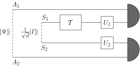
We now show how the optimal measurement can be experimentally implemented. Referring to Fig. 3, the bipartite system carrying the Choi operator of the transformation is indicated with the labels $S_{1}$ and $S_{2}$. We prepare a pair of ancillary systems $A_{1}$ and $A_{2}$ in the joint state $|\Psi\rangle\!\rangle\langle\!\langle\Psi|$, then we apply two random unitary transformations $U_{1}$ and $U_{2}$ to $S_{1}$ and $S_{2}$, finally we perform a Bell measurement on the pair $A_{1}S_{1}$ and another Bell measurement on the pair $A_{2}S_{2}$. This experimental scheme realizes the continuous measurement by randomizing among a continuous set of discrete POVM; this is a particular application of a general result proved in [101]. The scheme proposed is feasible using e. g. the Bell measurements experimentally realized in [100]. We note that choosing $|\Psi\rangle\!\rangle$ maximally entangled (as proposed for example in [60]) is generally not optimal, except for the unital case.

The experimental schemes for POVMs/states are obtained by removing the upper/lower for branch quantum operations, respectively. In the remaining branch the bipartite detector becomes mono-partite, performing a von Neumann measurement for the qudit, preceded by a random unitary in $SU(d)$. Moreover, for the case of POVM, the state $|\Psi\rangle\!\rangle$ is missing, whereas, for state-tomography, both bipartite states are missing. The optimal $\eta_{{\mathcal{E}},{\mathcal{G}}}$ in Eq. (67) is given by $\eta=d^{3}+d^{2}-d$, in both cases (for state-tomography compare with Ref. [76]).

References

- [1] M. G. A. Paris and J. Řeháček (Eds.) Quantum State Estimation, Lect. Notes Phys. 649 (Springer, Berlin-New York, 2004).
- [2] G. M. D’Ariano, L. Maccone, and M. F. Sacchi, Homodyne tomography and the reconstruction of quantum states of light, in Quantum Information with Continuous Variables of Atoms and Light, Ed. by N. Cerf, G. Leuchs, and E. Polzik, (Imperial College Press, London, 2007).
- [3] G. M. D’Ariano, M. G. A. Paris, M. F. Sacchi, Quantum Tomography, Advances in Imaging and Electron Physics 128 205-308 (2003)
- [4] P. Busch, Informationally complete sets of physical quantities, Int. J. Theor. Phys. 30, 1217 (1991).
- [5] G. M. D’Ariano, P. Perinotti, and M. F. Sacchi, Quantum Universal Detectors, Europhys. Lett. 65 165 (2004)
- [6] G. M. D’Ariano, P. Perinotti, and M. F. Sacchi, Informationally complete measurements and group representation, J. Opt. B: Quantum Semiclass. Opt. 6, S487-S491 (2004).
- [7] G. M. D’Ariano and P. Perinotti, Optimal Data Processing for Quantum Measurements, Phys. Rev. Lett. 98, 020403 (2007).
- [8] A. Bisio, G. Chiribella, G. M. D’Ariano, S. Facchini, and P. Perinotti, Optimal Quantum Tomography of States, Measurements, and Transformations, Phys. Rev. Lett. 102, 010404 (2009).
- [9] G. Chiribella, G. M. D’Ariano, and P. Perinotti, Quantum Circuit Architecture, Phys. Rev. Lett. 101, 060401 (2008).
- [10] U. Fano, Description of States in Quantum Mechanics by Density Matrix and Operator Techniques, Rev. Mod. Phys. 29, 74 (1957).
- [11] W. Pauli, in Encyclopedia of Physics V (Springer, Berlin 1958) p. 17.
- [12] W. Band and J. L. Park, The empirical determination of quantum states, Found. Phys. 1, 133 (1970).
- [13] B. D’Espagnat, Conceptual Foundations of Quantum Mechanics (W. A. Benjamin, Mass. 1976).
- [14] V. Bužek, Quantum tomography from incomplete data via MaxEnt principle, in Lect. Notes Phys. 649 189 (2004).
- [15] S. Olivares and M. G. A. Paris, Quantum estimation via the minimum Kullback entropy principle, Phys. Rev. A 76, 042120 (2007).
- [16] A. Royer, Measurement of quantum states and the Wigner function, Found. Phys. 19, 3 (1989).
- [17] D. T. Smithey, M. Beck, M. G. Raymer, and A. Faridani, Measurement of the Wigner distribution and the density matrix of a light mode using optical homodyne tomography - Application to squeezed states and the vacuum, Phys. Rev. Lett. 70, 1244 (1993).
- [18] K. Vogel and H. Risken, Determination of quasiprobability distributions in terms of probability distributions for the rotated quadrature phase, Phys. Rev. A 40, 2847 (1989).
- [19] G. M. D’Ariano, C. Macchiavello, and M. G. A. Paris, Detection of the density matrix through optical homodyne tomography without filtered back projection, Phys. Rev. A 50, 4298 (1994).
- [20] U. Leonhardt, H. Paul and G. M. D’Ariano, Tomographic reconstruction of the density matrix via pattern functions, Phys. Rev. A 52, 4899 (1995).
- [21] G. M. D’Ariano, Measuring Quantum States, in Quantum Optics and Spectroscopy of Solids, ed. by T. Hakioǧlu and A. S. Shumovsky, (Kluwer Academic Publisher, Amsterdam, 1997), p. 175-202.
- [22] M. Munroe, D. Boggavarapu, M. E. Anderson, and M. G. Raymer, Photon-number statistics from the phase-averaged quadrature-field distribution: Theory and ultrafast measurement, Phys. Rev. A 52, R924 (1995).
- [23] S. Schiller, G. Breitenbach, S. F. Pereira, T. Müller and J. Mlynek, Quantum statistics of the squeezed vacuum by measurement of the density matrix in the number state representation, Phys. Rev. Lett. 77 2933 (1996); G. Breitenbach, S. Schiller and J. Mlynek, Measurement of the quantum states of squeezed light, Nature 387, 471 (1997).
- [24] U. Janicke and M. Wilkens, Tomography of Atom Beams, J. Mod. Opt. 42, 2183 (1995); S. Wallentowitz and W. Vogel, Reconstruction of the Quantum Mechanical State of a Trapped Ion, Phys. Rev. Lett. 75, 2932 (1995); S. H. Kienle, M. Freiberger, W. P. Schleich, and M. G. Raymer in Experimental Metaphysics: Quantum Mechanical Studies for Abner Shimony ed. by S. Cohen et al. (Kluwer, Lancaster, 1997) p. 121.
- [25] T. J. Dunn, I. A. Walmsley and S. Mukamel, Experimental Determination of the Quantum-Mechanical State of a Molecular Vibrational Mode Using Fluorescence Tomography, Phys. Rev. Lett. 74, 884 (1995).
- [26] C. Kurtsiefer, T. Pfau T. and J. Mlynek, Measurement of the Wigner function of an ensemble of helium atoms, Nature 386, 150 (1997).
- [27] D. Leibfried, D. M. Meekhof, B. E. King, C. Monroe, W. M. Itano and D. J. Wineland, Experimental Determination of the Motional Quantum State of a Trapped Atom, Phys. Rev. Lett. 77, 4281 (1996).
- [28] G. M. D’Ariano, M. Vasilyev, and P. Kumar, Self-homodyne tomography of a twin-beam state, Phys. Rev. A 58, 636 (1998).
- [29] G. M. D’Ariano, Homodyning as universal detection, in Quantum Communication, Computing, and Measurement, edited by O. Hirota, A. S. Holevo, and C. M. Caves (Plenum Publishing, New York and London, 1997) p. 253.
- [30] G. D’Ariano, P. Kumar, M. Sacchi, Universal homodyne tomography with a single local oscillator, Phys. Rev. A 61, 13806 (2000).
- [31] G. M. D’Ariano, Latest developements in quantum tomography, in Quantum Communication, Computing, and Measurement, edited by P. Kumar, G. M. D’Ariano, and O. Hirota (Kluwer Academic/Plenum Publishers, New York and London, 2000) p. 137.
- [32] G. M. D’Ariano, Universal quantum estimation, Phys. Lett. A 268, 151 (2000).
- [33] G. Cassinelli, G. M. D’Ariano, E. De Vito, A. Levrero, Group TheoreticalQuantum Tomography, J. Math. Phys. 41, 7940 (2000)
- [34] G. M. D’Ariano, L. Maccone, and M. G. A. Paris, Orthogonality relations in Quantum Tomography, Phys. Lett. A 276, 25 (2000)
- [35] G. M. D’Ariano, L. Maccone and M. G. A. Paris, Quorum of observables for universal quantum estimation, J. Phys. A: Math. Gen. 34, 93 (2001).
- [36] E. Prugovečki, Information-theoretical aspects of quantum measurement,Int. J. Theor. Phys 16, 321 (1977).
- [37] Z. Hradil, Quantum-state estimation, Phys. Rev. A 55, R1561 (1997).
- [38] K. Banaszek, Maximum-likelihood estimation of photon-number distribution from homodyne statistics Phys. Rev. A 57, 5013 (1998).
- [39] K. Banaszek, G. M. D’Ariano, M. G. A. Paris, M. F. Sacchi, Maximum-likelihood estimation of the density matrix, Phys. Rev. A 61 010304(R) (2000).
- [40] R. Blume-Kohout, Optimal, reliable estimation of quantum states, quant-ph/0611080.
- [41] I. L. Chuang and M. A. Nielsen, Prescription for experimental determination of the dynamics of a quantum black box, J. Mod. Opt. 44, 2455 (1997).
- [42] J. F. Poyatos, J. I. Cirac, and P. Zoller, Complete Characterization of a Quantum Process: The Two-Bit Quantum Gate, Phys. Rev. Lett. 78, 390 (1997).
- [43] G. M. D’Ariano and L. Maccone, Measuring Quantum Optical Hamiltonians, Phys. Rev. Lett. 80, 5465 (1998).
- [44] G. M. D’Ariano and P. Lo Presti, Quantum Tomography for Measuring Experimentally the Matrix Elements of an Arbitrary Quantum Operation, Phys. Rev. Lett. 86, 4195 (2001).
- [45] D. Leung, Ph.D. thesis, Stanford University, comp-sci/0012017.
- [46] M. F. Sacchi, Maximum-likelihood reconstruction of completely positive maps, Phys. Rev. A 63, 054104 (2001).
- [47] G. D’Ariano and P. Lo Presti, Imprinting a complete information about a quantum channel on its output state, Phys. Rev. Lett. 91, 047902 (2003).
- [48] J. B. Altepeter, D. Branning, E. Jeffrey, T. C. Wei, P. G. Kwiat, R. T. Thew, J. L. O’Brien, M. A. Nielsen, and A. G. White, Ancilla-Assisted Quantum Process Tomography, Phys. Rev. Lett. 90, 193601 (2003).
- [49] G. M. D’Ariano, P. Lo Presti, and L. Maccone, Quantum Calibration of Measurement Instrumentation, Phys. Rev. Lett. 93, 250407 (2004).
- [50] G. M. D’Ariano and P. Lo Presti, Characterization of Quantum Devices, Lect. Notes Phys. 649, 297-322 (Springer, Berlin-New York 2004).
- [51] G. M. D’Ariano, M. G. A. Paris, and M. F. Sacchi, Quantum Tomographic Methods, Lect. Notes Phys. 649, 2-58 (Springer, Berlin-New York 2004).
- [52] J. Fiurášek and Z. Hradil, Maximum-likelihood estimation of quantum processes, Phys. Rev. A 63, 020101(R) (2001).
- [53] J. Fiurášek, Maximum-likelihood estimation of quantum measurement, Phys. Rev. A 64 024102 (2001).
- [54] A. Luis and L. L. Sanchez-Soto, Complete Characterization of Arbitrary Quantum Measurement Processes, Phys. Rev. Lett. 83, 3573 (1999).
- [55] G. M. D’Ariano, Universal quantum observables, Phys. Lett. A 300, 1 (2002).
- [56] A. M. Childs, I. L. Chuang, D. W. Leung, Realization of quantum process tomography in NMR, Phys. Rev. A 64, 012314 (2001).
- [57] F. de Martini, A. Mazzei, M. Ricci, G. M. D’Ariano, Exploiting quantum parallelism of entanglement for a complete experimental quantum characterization of a single-qubit device, Phys. Rev. A 67, 062307 (2003).
- [58] M. Mohseni and D. A. Lidar, Direct Characterization of Quantum Dynamics, Phys. Rev. Lett. 97, 170501 (2006).
- [59] M. Mohseni and D. A. Lidar, Direct characterization of quantum dynamics: General theory, Phys. Rev. A 75, 062331 (2007).
- [60] M. Mohseni, A. T. Rezakhani, and D. A. Lidar, Quantum-process tomography: Resource analysis of different strategies, Phys. Rev. A 77, 032322 (2008).
- [61] A. Bendersky, F. Pastawski, J. P. Paz, Selective and Efficient Estimation of Parameters for Quantum Process Tomography, Phys. Rev. Lett. 100, 190403 (2008).
- [62] P. Delsarte, J. M. Goethals, and J. J. Seidel, Spherical codes and designs, Geometriae Dedicata 6, 363 (1977).
- [63] M. Lobino, D. Korystov, C. Kupchak, E. Figueroa, B. C. Sanders, and A. I. Lvovsky, Complete Characterization of Quantum-Optical Processes, Science 322, 563 (2008).
- [64] J. S. Lundeen, A. Feito, H. Coldenstrodt-Ronge, K. L. Pregnell, C. Silberhorn, T. C. Ralph, J. Eisert, M. B. Plenio, I. A. Walmsley, Tomography of quantum detectors, Nature Physics 5, 27 (2008).
- [65] S. H. Myrskog, J. K. Fox, M. W. Mitchell, and A. M. Steinberg, Quantum process tomography on vibrational states of atoms in an optical lattice, Phys. Rev. A 72, 013615 (2005).
- [66] M. Riebe, M. Chwalla, J. Benhelm, H. Häffner, W. Hänsel, C. F. Roos, and R. Blatt, Quantum teleportation with atoms: quantum process tomography, New. J. Phys. 9, 211 (2007).
- [67] H. Kampermann and W. S. Veeman, Characterization of quantum algorithms by quantum process tomography using quadrupolar spins in solid-state nuclear magnetic resonance, J. Chem. Phys. 122, 214108 (2005).
- [68] M. Howard, J. Twamley, C. Wittmann, T. Gaebel, F. Jelezko, and J. Wrachtrup, Quantum process tomography and Linblad estimation of a solid-state qubit, New J. Phys. 8, 33 (2006).
- [69] M. Brune, J. Bernu, C. Guerlin, S. Deléglise, C. Sayrin, S. Gleyzes, S. Kuhr, I. Dotsenko, J. M. Raimond, and S. Haroche, Process Tomography of Field Damping and Measurement of Fock State Lifetimes by Quantum Nondemolition Photon Counting in a Cavity, Phys. Rev. Lett. 101, 240402 (2008).
- [70] P. Shor, Scheme for reducing decoherence in quantum computer memory, Phys. Rev. A 52, R2493 (1995).
- [71] A. M. Steane, Error Correcting Codes in Quantum Theory, Phys. Rev. Lett. 77, 793 (1996).
- [72] E. Knill and R. Laflamme, Theory of quantum error-correcting codes, Phys. Rev. A 55, 900 (1997).
- [73] M. W. Mitchell, C. W. Ellenor, R. B. A. Adamson, J. S. Lundeen, A. M. Steinberg, Quantum process tomography and the search for decoherence-free subspaces, in Quantum Information and Computation II. E. Donkor, A. R. Pirich, R. Andrew, H. E. Brandt eds., Proceedings of the SPIE, 5436, 223-231 (2004).
- [74] J. Emerson, M. Silva, O. Moussa, C. Ryan, M. Laforest, J. Baugh, D. G. Cory, and R. Laflamme, Symmetrized Characterization of Noisy Quantum Processes, Science 317, 1893 (2007)
- [75] R. L. Kosut, Quantum Process Tomography via L1-norm Minimization, arXiv:0812.4323.
- [76] A. J. Scott, Tight informationally complete quantum measurements, J. Phys. A 39, 13507 (2006).
- [77] C. W. Helstrom, Quantum detection and estimation theory, (Academic Press, New York, San Francisco, London, 1976).
- [78] G. Chiribella, G. M. D’Ariano, and P. Perinotti, Memory Effects in Quantum Channel Discrimination, Phys. Rev. Lett. 101, 180501 (2008).
- [79] M. Ziman, Incomplete quantum process tomography and principle of maximal entropy, Phys. Rev. A 78, 032118 (2008).
- [80] R. B. Bhapat, Linear Algebra and Linear Models, (Springer-Verlag, New York, 2000).
- [81] R. J. Duffin and A. C. Schaeffer, A class of nonharmonic Fourier series, Trans. Am. Math. Soc. 72, 341 (1952).
- [82] S. Li, On general frame decompositions, Numer. Funct. Anal. Optim. 16 1181 (1995).
- [83] G. M. D’Ariano, M. F. Sacchi, Renormalized quantum tomography arXiv:0901.2866
- [84] G. M. D’Ariano, D. F. Magnani, and P. Perinotti, Adaptive Bayesian and frequentist data processing for quantum tomography Phys. Lett. A, doi:10.1016/j.physleta.2009.01.055.
- [85] P. G. Casazza, D. Han, and D. Larson, Frames for Banach spaces, Contemp. Math. 247, 149-182 (1999).
- [86] C. M. Caves, C. A. Fuchs, and R. Schack, Unknown quantum states: The quantum de Finetti representation, J. Math. Phys. 43, 4537 (2002).
- [87] G. M. D’Ariano, P. Perinotti, and M. F. Sacchi, Quantum indirect estimation theory and joint estimates of all moments of two incompatible observables, Phys. Rev. A 77, 052108 (2008).
- [88] G. M. D’Ariano, P. Perinotti, and M. F. Sacchi, Informationally complete measurements on bipartite quantum systems: Comparing local with global measurements, Phys. Rev. A 72, 042108 (2005).
- [89] G. M. D’Ariano, L. Maccone, and M. Paini, Spin tomography, J. Opt. B 5, 77 (2003).
- [90] G. M. D’Ariano, E. De Vito, and L. Maccone, SU (1,1) tomography, Phys. Rev. A 64, 033805 (2001).
- [91] G. Chiribella, G. M. D’Ariano, and P. Perinotti, Applications of the group SU (1,1) for quantum computation and tomography, Laser Phys. 16, 1572 (2006).
- [92] A. Grossmann, J. Morlet, and T. Paul, Transforms associated to square integrable group representations. I: General results., J. Math. Phys. 26, 2473 (1985).
- [93] G. M. D’Ariano, P. Perinotti, and M. F. Sacchi, Optimization of Quantum Universal Detectors, in Squeezed States and Uncertainty Relations, ed. by H. Moya-Cessa, R. Jauregui, S. Hacyan, and O. Castanos, (Rinton Press, Princeton, 2003) pag. 86.
- [94] G. M. D’Ariano, Tomographic methods for universal estimation in quantum optics, Scuola “E. Fermi” on Experimental Quantum Computation and Information, F. De Martini and C. Monroe ed. (IOS Press, Amsterdam, 2002) pag. 385.
- [95] G. M. D’Ariano, and N. Sterpi, Robustness of Homodyne Tomography to Phase-Insensitive Noise, J. Mod. Optics 44 2227 (1997).
- [96] G. M. D’Ariano and P. Perinotti, Optimal estimation of ensemble averages from a quantum measurement, in Proceedings of the 8th Int. Conf. on Quantum Communication, Measurement and Computing, ed. by O. Hirota, J. H. Shapiro and M. Sasaki (NICT press, Japan, 2007), p. 327.
- [97] G. Chiribella, G. M. D’Ariano, and P. Perinotti, Transforming quantum operations: quantum supermaps, Europhys. Lett. 83, 30004 (2008).
- [98] A. S. Holevo, Probabilistic and Statistical Aspects of Quantum Theory, North Holland, Amsterdam, 1982.
- [99] A. J. Scott, Optimizing quantum process tomography with unitary 2-design, J. Phys. A 41, 055308 (2008).
- [100] P. Walther, A. Zeilinger, Experimental Realization of a Photonic Bell-State Analyzer, Phys. Rev. A 72, 010302(R) (2005)
- [101] G. Chiribella, G. M. D’Ariano, D. M. Schlingemann, How continuous quantum measurements in finite dimension are actually discrete, Phys. Rev. Lett. 98, 190403 (2007).