Nonlinear TM Modes of the Symmetric Hyperbolic Slab Waveguide

Abstract

Guided wave modes in a symmetric slab waveguide formed by an isotropic dielectric layer with cubic nonlinear response placed in the hyperbolic surrounding medium are investigated theoretically. Optical axis of the hyperbolic medium is normal to the slab plane. If dielectric permittivity of the waveguide core is more than extraordinary permittivity of the hyperbolic medium each TM mode has two cut-off frequencies. The dispersion relations for these modes are found and numerically solved for cases of focusing and defocussing medium of the core. Number of possible modes at given frequency depends on the applied field intensity. It is shown that zero values of the TM modes propagation constants are possible in the waveguide. Moreover in the self-defocussing case they can be obtained by increasing field intensity. The dependence of a propagation constant and width of the mode on radiation intensity is obtained and analyzed.

I Introduction

Hyperbolic medium can be defined as strongly anisotropic uniaxial medium which principal components of dielectric permittivity or magnetic permeability tensors have opposite signs Narim:06 ; Noginov:09 . In case of nonmagnetic hyperbolic material an extraordinary wave propagating through this medium has a hyperbolic dispersion. This lead to a number of new optical phenomena Poddubny:12 ; Poddubny:13 ; Ferrari:14 ; Benedict:13 ; Zapata:13 ; XNi:11 . A review is presented in Drachev:13 ; Shekhar:14 .

Photonic or plasmonic guiding devices, such as waveguides, are widely used in different communication networks or information processing systems. A numerous guiding structures formed from hyperbolic medium as component were investigated already. Among them are plasmonic waveguides with hyperbolic cladding Kildishev:15a ; Kildishev:15b , photonic waveguides with hyperbolic core Huang:08 ; Zhu:15 or surroundings Guo-ding Xu:08 demonstrating negative refractive index, slow light, large mode index, etc. All these works are limited by linear media response to the applied radiation.

In our previous work Lyashko:15 a slab waveguide with isotropic dielectric core in the hyperbolic host was considered. In this structure much of the guided wave energy is concentrated in the non-dissipative core, whereas only evanescent waves are in the hyperbolic medium. The optical axis of hyperbolic medium is aligned with normal vector to the wave propagation direction. In this geometry the transverse magnetic polarization modes is extraordinary waves in the hyperbolic cladding. This leads to the new phenomenon: each TM guiding wave could be characterized by the two cut-off frequencies. Thus, each TM mode is held by the waveguide only in certain frequency range or the mode exists only in certain interval of core thickness. It is conventional only one cut-off frequency exists and the number of the guided waves is always increasing with the frequency or the core thickness.

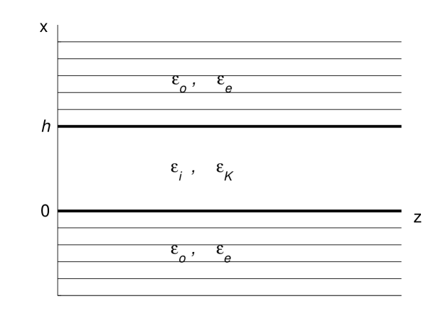
Figure 1: Scheme of hyperbolic slab waveguide

Nonlinear guided wave modes in an asymmetric slab waveguide formed by an isotropic dielectric layer placed on a linear or nonlinear substrate and covered by a hyperbolic material were investigated in LM:16 . In this case the additional solutions for guided waves arises. These modes corresponds with situation, where the peak of electric field is localized in the nonlinear substrate. These modes are absent in the linear waveguide. To excite these modes the power must exceed certain threshold value. The cut-off frequencies for each mode are determined by the dielectric permittivities and the field intensity.

In present paper the nonlinear guided wave modes in an symmetric slab waveguide formed by an isotropic nonlinear dielectric layer dipped into a hyperbolic material will be considered.

In the next step we will consider a cubic nonlinear response of the core medium and its influence on the waveguide dispersion characteristics. The field distributions and dispersion relations, connecting mode propagation constant and radiation frequency, are analytically obtained and analyzed. Cases of self-focusing and self-defocusing Kerr medium of the core are considered. In all cases the two cutoff frequencies phenomenon also exist. In the case of focusing core medium mode effective refractive index (or propagation constant) increases with field intensity growth. In the de-focusing case propagation constant monotonically decreases with intensity growth, achieving zero value. This situation equals to zero energy flux in the mode propagation direction or ”stopped light”. Also it is possible to control a number of propagating modes in the hyperbolic waveguide varying the field intensity. There is another phenomenon in case of self-defocusing core in the hyperbolic environment, namely, the mode width narrows with field intensity growth.

II Constituent Equations

It is assumed that waveguide under consideration is formed by nonmagnetic media without any dissipation. The substrate and the covering layer are uniaxial hyperbolic media with an optical axis directed perpendicularly to the media interfaces. An electromagnetic properties of the hyperbolic media are described by principle components of the dielectric tensor: $\varepsilon_{o}$ and $\varepsilon_{e}$. The core is a cubic nonlinear (Kerr) isotropic dielectric characterized by linear dielectric permittivity $\varepsilon_{i}$ and Kerr constant $\varepsilon_{K}$. The coordinate axes are determined as follows. OX axis is directed along with the normal vector to the interfaces. OY and OZ axes are parallel to the core interfaces. It is assumed that guided waves propagate along the OZ axis. In such planar geometry the electromagnetic fields are independent on the y coordinate.

To describe an electromagnetic wave propagation in the general case following system can be obtained from the wave equations Lyashko:15 ; LM:16

$$\left(\frac{\varepsilon_{e}(x)}{\varepsilon_{o}(x)}\frac{\partial^{2}}{\partial x^{2}}+\frac{\partial^{2}}{\partial z^{2}}+k_{0}^{2}\varepsilon_{e}(x)\right)E_{x}+4\pi k_{0}^{2}P_{nl,x}=0,$$

$$\left(\frac{\partial^{2}}{\partial x^{2}}+\frac{\partial^{2}}{\partial z^{2}}+k_{0}^{2}\varepsilon_{o}(x)\right)E_{y}+4\pi k_{0}^{2}P_{nl,y}=0,$$ (1)

$$\left(\frac{\partial^{2}}{\partial x^{2}}+\frac{\partial^{2}}{\partial z^{2}}+k_{0}^{2}\varepsilon_{o}(x)\right)E_{z}+\frac{\Delta\varepsilon(x)}{\varepsilon_{o}(x)}\frac{\partial^{2}}{\partial x\partial z}E_{x}+$$

$$\qquad\qquad\qquad\qquad\qquad+4\pi k_{0}^{2}P_{nl,z}=0.$$

If planar waveguide with core width $h$ is considered, linear principal dielectric constants can be presented as piecewise functions

$$\varepsilon_{o,e}(x)=\left\{\begin{array}[]{ccc}\varepsilon_{o,e}&~{}~{}x<0,\\ \varepsilon_{i}&~{}~{}0\leq x\leq h,\\ \varepsilon_{o,e}&~{}~{}x>h,\\ \end{array}\right.$$ (2)

In the planar geometry under consideration (Fig. 1) transverse electric (TE) and transverse magnetic (TM) waves can be analyzed independently. The present work is dedicated to TM polarization case. TM wave is an extraordinary wave and is defined by following field components $\mathbf{E}=(E_{x},0,E_{z})$ and $\mathbf{H}=(0,H_{y},0)$. These components are connected with each other

$$H_{y} = \frac{i}{k_{0}}\left(\frac{\partial E_{z}}{\partial x}-\frac{\partial E_{x}}{\partial z}\right),$$

$$\frac{\partial H_{y}}{\partial z} = ~{}~{}~{}ik_{0}\varepsilon_{e}(x)E_{x}+i4\pi k_{0}P_{nl,x},$$ (3)

$$\frac{\partial H_{y}}{\partial x} = -ik_{0}\varepsilon_{o}(x)E_{z}-i4\pi k_{0}P_{nl,z}.$$

It is assumed that no harmonic generation processes available in the waveguide core. Nonlinear polarization for TM wave in case of isotropic core medium can be presented as

$$P_{x}^{nl}=(\gamma_{xx}|E_{x}|^{2}+\gamma_{xz}|E_{z}|^{2})E_{x},$$

$$P_{z}^{nl}=(\gamma_{zz}|E_{z}|^{2}+\gamma_{zx}|E_{x}|^{2})E_{z},$$

where parameters $\gamma_{ij}$ depend on forth-rank susceptibility tensor components $\chi_{mnkl}$. In further analysis for simplicity we will consider uniaxial approximation Mihala:Fedy:83 ; Agranowich:86 $\gamma_{zz}=\varepsilon_{K}/4\pi$, $\gamma_{xz}=\gamma_{zx}=\gamma_{xx}=0$. Thus, an expression for nonlinear polarization will take a form:

$$\textbf{P}^{nl}=\frac{\varepsilon_{K}}{4\pi}|E_{z}|^{2}E_{z}\textbf{e}_{z}.$$ (4)

III Electromagnetic Field Distribution

The considered waveguide is homogeneous in $Z$ direction. So the guiding wave fields can be presented as $\mathbf{E}=(\tilde{E}_{x},0,\tilde{E}_{z})e^{i\beta z}$ and $\mathbf{H}=(0,\tilde{H}_{y},0)e^{i\beta z}$, where $\beta$ is propagation constant. In this assumption one can obtain from (1) the following system for the $\tilde{E}_{z}$ component

$$x<0 \frac{\partial^{2}}{\partial x^{2}}\tilde{E}_{z}+\frac{\varepsilon_{o}}{\varepsilon_{e}}(k_{0}^{2}\varepsilon_{e}-\beta^{2})\tilde{E}_{z}=0,$$

$$0\leq x\leq h \frac{\partial^{2}}{\partial x^{2}}\tilde{E}_{z}+(k_{0}^{2}\varepsilon_{i}-\beta^{2})\tilde{E}_{z}+k_{0}^{2}\varepsilon_{K}\tilde{E}_{z}^{3}=0,$$ (5)

$$x>h \frac{\partial^{2}}{\partial x^{2}}\tilde{E}_{z}+\frac{\varepsilon_{o}}{\varepsilon_{e}}\left(k_{0}^{2}\varepsilon_{e}-\beta^{2}\right)\tilde{E}_{z}=0,$$

It is suitable to introduce new parameters $q^{2}=\varepsilon_{o}/\varepsilon_{e}(\beta^{2}-k_{0}^{2}\varepsilon_{e})$, $p^{2}=k_{0}^{2}\varepsilon_{i}-\beta^{2}$. To consider guided modes of the waveguide the condition $q^{2}>0$ must be satisfied. In the case of a hyperbolic material this inequality is satisfied only when $\varepsilon_{o}<0$ and $\varepsilon_{e}>0$.

There is no restriction for the $p^{2}$ sign. The case of $p^{2}<0$ corresponds to pair of two surface waves propagating along the waveguide interfaces. The case $p^{2}>0$ corresponds to guided modes regime of the waveguide. In further analysis the case $p^{2}>0$ will be considered.

The first and the last equations of the system (5) can be simply integrated

$$\tilde{E}_{z}^{(1)}=A_{0}e^{qx},\quad\tilde{E}_{z}^{(3)}=A_{h}e^{-qx},$$ (6)

The upper marks 1 and 3 are referred to substrate and covering layer respectively.

The second equation of (5) can be integrated in terms of Jacobi elliptic functions Batm:Erd:67 . The first step is to present (5) as an integral of motion

$$\left(\frac{\partial}{\partial x}\tilde{E}_{z}\right)^{2}+p^{2}\tilde{E}_{z}^{2}+\frac{1}{2}k_{0}^{2}\varepsilon_{K}\tilde{E}_{z}^{4}=G,$$ (7)

where $G$ is an integration constant.

In further derivation we will concentrate on case of the self-defocusing core medium, $\varepsilon_{K}<0$. Case of self-focusing medium could be described in similar way.

By introducing a new variable $v=\sqrt{\alpha}\tilde{E}_{z}$, where $\alpha=\sqrt{k_{0}^{2}|\varepsilon_{K}|/2}$ is a new parameter of nonlinearity, one can obtain from the (7)

$$\left(\frac{\partial v}{\partial x}\right)^{2}=\alpha(v^{2}-\bar{v}_{1}^{2})(v^{2}-\bar{v}_{2}^{2}).$$ (8)

Here $\bar{v}_{1}^{2}$, $\bar{v}_{2}^{2}$ are

$$\bar{v}_{1}^{2}=\frac{p^{2}}{2\alpha}-\sqrt{\left(\frac{p^{2}}{2\alpha}\right)^{2}-G},~{}~{}~{}\bar{v}_{2}^{2}=\frac{p^{2}}{2\alpha}+\sqrt{\left(\frac{p^{2}}{2\alpha}\right)^{2}-G}.$$

By the use of $w(x)=v(x)/\bar{v}_{1}$ the equation (8) can be presented as

$$\left(\frac{\partial w}{\partial x}\right)^{2}=\alpha\bar{v}_{2}^{2}(1-w^{2})(1-\xi^{2}w^{2}),$$ (9)

where $\xi^{2}=\bar{v}_{1}^{2}/\bar{v}_{2}^{2}$, $0\leq\xi^{2}\leq 1$, and $\xi$ monotonically increases with $G$. Hence parameter $\xi$ can be considered as a new integration constant. Parameters in (8) can be presented in terms of $\xi$

$$\bar{v}_{1}^{2}=\frac{p^{2}}{\alpha}\frac{\xi^{2}}{1+\xi^{2}},~{}~{}~{}~{}\bar{v}_{2}^{2}=\frac{p^{2}}{\alpha}\frac{1}{1+\xi^{2}}.$$

By integrating (9) one obtains the expression

$$\pm\frac{p(x-x_{0})}{\sqrt{1+\xi^{2}}}=\int_{0}^{w}\frac{d\tilde{w}}{\sqrt{(1-\tilde{w}^{2})(1-\xi^{2}\tilde{w}^{2})}},$$ (10)

where $x_{0}$ is integration constant. Integral in the right side of the equation is the incomplete elliptic integral of the first genus Batm:Erd:67 . Hence $w$ can be expressed in terms of the Jacobi elliptic sinus

$$w(x)=\pm\mathrm{sn}\left(\frac{p(x-x_{0})}{\sqrt{1+\xi^{2}}},~{}\xi\right).$$

Z-component of electric field in the core of waveguide is defined as

$$\tilde{E}_{z}^{(2)}=\frac{\bar{v}_{1}}{\sqrt{\alpha}}w(x)=\pm\frac{p}{\alpha}\frac{\xi}{\sqrt{1+\xi^{2}}}~{}\mathrm{sn}\left(\frac{p(x-x_{0})}{\sqrt{1+\xi^{2}}};~{}\xi\right).$$

It is suitable to introduce a new variable

$$A_{m}=\frac{p}{\alpha}\frac{\xi}{\sqrt{1+\xi^{2}}},$$ (11)

which is the maximum value of field component $E_{z}$.

As is known, tangential components of electric and magnetic fields are continuous functions on the boundaries between media. Taking into account the equations (6) for electric fields in the substrate and in the cover, the following definitions can be achieved

$$x<0 \tilde{E}^{(1)}_{z}(x)=\pm A_{m}~{}\mathrm{sn}\left(\frac{-px_{0}}{\sqrt{1+\xi^{2}}};~{}\xi\right)e^{qx},$$

$$0\leq x\leq h \tilde{E}^{(2)}_{z}(x)=\pm A_{m}~{}\mathrm{sn}\left(\frac{p(x-x_{0})}{\sqrt{1+\xi^{2}}};~{}\xi\right),$$ (12)

$$x>h \tilde{E}^{(3)}_{z}(x)=\pm A_{m}~{}\mathrm{sn}\left(\frac{p(h-x_{0})}{\sqrt{1+\xi^{2}}};~{}\xi\right)e^{q(h-x)},$$

so $\tilde{E}_{z}^{(1)}(0)=\tilde{E}_{z}^{(2)}(0)$ and $\tilde{E}_{z}^{(2)}(h)=\tilde{E}_{z}^{(3)}(h)$. The upper marks 1, 2 and 3 are referred to substrate, core and covering layer.

In the case of self-focusing core medium the Z-components of electric field distribution can be obtained by the use of substitution $\xi=i\kappa$, where $0\leq\kappa\leq 1$.

Components of $\tilde{H}_{y}$ and $\tilde{E}_{x}$ can be easy expressed in terms of $\tilde{E}_{z}$ using the following formulas:

$$\tilde{H}_{y}=\frac{ik_{0}\varepsilon_{e}(x)}{k_{0}^{2}\varepsilon_{e}(x)-\beta^{2}}\frac{\partial}{\partial x}\tilde{E}_{z},$$

(13)

$$\tilde{E}_{x}=\frac{i\beta}{k_{0}^{2}\varepsilon_{e}(x)-\beta^{2}}\frac{\partial}{\partial x}\tilde{E}_{z},$$

that follow from the system (3) and assumption (4).

It is important to understand how the system (12) can be transformed to the linear case. Let us consider the case when $\varepsilon_{K}$ is negligibly small. Thus parameter $\xi$ will be:

$$\xi^{2}=\frac{p^{2}-\sqrt{p^{4}-G(2\alpha)^{2}}}{p^{2}+\sqrt{p^{4}-G(2\alpha)^{2}}}~{}\to 0~{}~{}(\alpha\to 0).$$

Then

$$\mathrm{sn}(p(x-x_{0});~{}0)~{}\to\sin(p(x-x_{0})).$$

So maximum value of $\tilde{E}_{z}^{(1,2,3)}=A_{m}$ will be

$$A_{m}^{2}=\frac{p^{2}}{\alpha^{2}}\frac{\xi^{2}}{1+\xi^{2}}~{}\to~{}\frac{G}{p^{2}},$$ (14)

where the definition of $\xi$ and L’Hôpital’s rule were used. Hence, $G$ is connected with maximum field intensity in the linear case.

IV Dispersion Relation

Taking into account the continuity conditions for $\tilde{H}_{y}$ at the core boundaries ($x=0$, $x=h$), equations (13) and system (12) the following relations can be achieved

$$\qquad\qquad\qquad-\frac{\varepsilon_{o}}{\varepsilon_{i}}\frac{p}{q}\sqrt{1+\xi^{2}}=$$

$$\frac{\mathrm{cn}\left(-px_{0}/\sqrt{1+\xi^{2}};\xi\right)\mathrm{dn}\left(-px_{0}/\sqrt{1+\xi^{2}};~{}\xi\right)}{\mathrm{sn}\left(-px_{0}/\sqrt{1+\xi^{2}};\xi\right)},$$

(15)

$$\qquad\qquad\qquad\frac{\varepsilon_{o}}{\varepsilon_{i}}\frac{p}{q}\sqrt{1+\xi^{2}}=$$

$$\frac{\mathrm{cn}\left(p(h-x_{0})/\sqrt{1+\xi^{2}};\xi\right)\mathrm{dn}\left(p(h-x_{0})/\sqrt{1+\xi^{2}};~{}\xi\right)}{\mathrm{sn}\left(p(h-x_{0})/\sqrt{1+\xi^{2}};\xi\right)}.$$

Comparison of the equations of this system results in the relation $x_{0}=h/2+NT\sqrt{1+\xi^{2}}/p$, where $T$ is a period of elliptic function $\mathrm{sn}(x,\xi)$ and $N$ is an integer constant. Periods of the elliptic functions $\mathrm{sn}(x,\xi)$ and $\mathrm{cn}(x,\xi)$ are the same. Period of $\mathrm{dn}(x,\xi)$ is equal to $T/2$. Thus the system (15) can be reduced to one equation

$$\qquad\qquad\qquad\frac{\varepsilon_{o}}{\varepsilon_{i}}\frac{p}{q}\sqrt{1+\xi^{2}}=$$ (16)

$$=\frac{\mathrm{cn}\left(ph/2\sqrt{1+\xi^{2}};~{}\xi\right)\mathrm{dn}\left(ph/2\sqrt{1+\xi^{2}};~{}\xi\right)}{\mathrm{sn}\left(ph/2\sqrt{1+\xi^{2}};~{}\xi\right)}.$$

This equation connects propagation constant $\beta$ included in parameters $p$ and $q$ with radiation frequency $\omega$ included in the wave number $k_{0}$. Hence obtained equation is the dispersion relation. The substitution $\xi=i\kappa$ results in the dispersion relation for the self-focusing core medium case, $\varepsilon_{K}>0$.

Parameter $\xi$ accounts nonlinear property of the waveguide core. As follows from (11) its value increases with intensity $A_{m}^{2}$.

In the linear case, $\xi=0$, elliptic functions are replaced by theirs trigonometrical analogous and relation (16) reduces to the dispersion equation obtained earlier LM:16 .

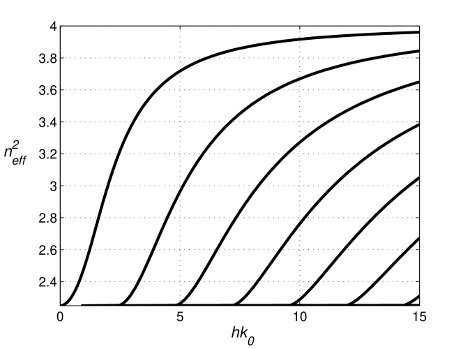
Figure 2: Dispersion curves for TM modes of the standard dielectric waveguide. Mode marks are: $m=0,1,2,3,4,5$.

In further analysis we will consider the mode effective refractive index $n_{eff}=\beta/k_{0}$ instead of mode propagation constant $\beta$. In the previous section it was shown that propagation parameters $q$ and $p$ must satisfy inequalities $q^{2}>0$, $p^{2}>0$. In the case of hyperbolic claddings with dielectric constants $\varepsilon_{o}<0$, $\varepsilon_{e}>0$ these conditions set limits on possible values of $n_{eff}$:

$$0\leq n_{eff}^{2}\leq\min{(\varepsilon_{e},\varepsilon_{i})},$$ (17)

were value $n_{eff}=0$ means zero value of wave vector projection on the mode propagation direction ($Z$ axis), i.e. stopped wave between the waveguide claddings. For comparison in the usual case of waveguide with dielectric claddings possible values of $n_{eff}$ are in the range

$$\varepsilon_{e}\leq n_{eff}^{2}\leq\varepsilon_{i}.$$ (18)

It is interesting to note that value $n_{eff}=\varepsilon_{i}$ or $p=0$ is a solution of dispersion relations both for hyperbolic and standard dielectric waveguide cases for all values of frequency or core width $h$. The elliptic functions presented in (16) are the periodic functions excepting the case $\xi=1$. Thus equation (16) has a number of different solution brunches $n_{eff}^{2}(hk_{0})$ that are dispersion characteristics for the different waveguide modes. They are usually marked with integer mode mark $m$. If the value $n_{eff}^{2}=\varepsilon_{i}$ is possible it will be at least one mutual point for all brunches. In Fig.2 the dispersion curves for TM modes of a usual linear dielectric slab waveguide with $\varepsilon_{i}=4.0$, $\varepsilon_{e}=\varepsilon_{o}=2.25$ are presented. One can notice that each TM mode curve have a starting point (cutoff frequency) where $n_{eff}^{2}=\varepsilon_{e}$ and then tends to the common value $n_{eff}^{2}=\varepsilon_{i}$ that is achieved at $hk_{0}\to\infty$. In the hyperbolic waveguide case at $\varepsilon_{e}<\varepsilon_{i}$, the value $n_{eff}^{2}=\varepsilon_{i}$ is not possible due to (18) and the behavior of dispersion curves is quite different.

(a) $\xi=0$

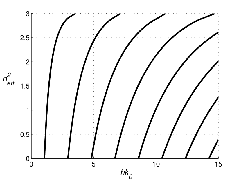
(b) $\xi=0.5$

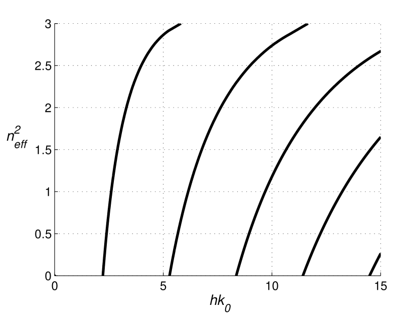
(c) $\xi=0.9$

Figure 3: Dispersion curves for TM modes in case of $\varepsilon_{K}<0$, $\varepsilon_{e}<\varepsilon_{i}$. Mode marks are: (a) $m$ = 1, 2,…, 9, (b) $m$ = 1, 2,…, 8, (c) $m$ = 1, 2,…, 5

.

Functions $n_{eff}^{2}(hk_{0})$ that are numerical solutions of the relation (16) are presented in Fig. 3 for different values of $\xi$. Linear dielectric permittivities of the waveguide layers are $\varepsilon_{i}=4.0$, $\varepsilon_{e}=3.0$, $\varepsilon_{o}=-3.5$. In several works Guo-ding Xu:08 ; Lyashko:15 it was shown that in the waveguide with hyperbolic environment there is not a fundamental mode corresponding to $m=0$. So in each case presented in Fig. 3 mode index starts from $m=1$ value.

From the pictures presented in Fig.3 it follows that TM modes in each case have two cutoff frequencies. At $n_{eff}^{2}(hk_{0})=0$ the mode appears in the waveguide, at $n_{eff}^{2}(hk_{0})=\varepsilon_{e}$ the mode leaves the waveguide. That is not possible in the usual dielectric waveguides. An additional cutoff frequency phenomenon found earlier in the linear case Lyashko:15 is present in the case of waveguide with nonlinear core too.

By comparing results presented on pictures of Fig.3 (a), (b), and (c) one can notice that with nonlinear parameter $\xi$ growth the density of dispersion characteristics becomes lower and each curve shifts to the greater values of normalized core width (or frequency). This allows to make conclusion that with intensity growth in the self-defocusing case an effective mode index $n_{eff}$ or propagation constant $\beta$ decreases and finally achieves zero value (for constant frequency value). Then mode leaves the waveguide. A case $\beta=0$ equals to the stopped waveguide mode.

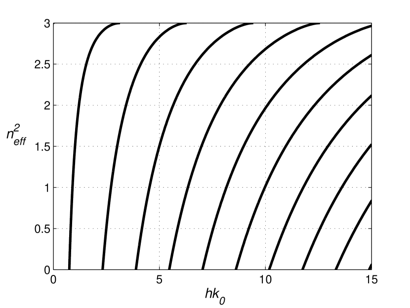
(a) $\kappa=0$

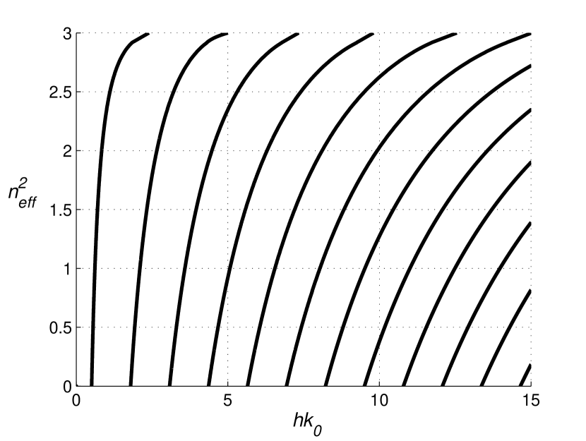
(b) $\kappa=0.5$

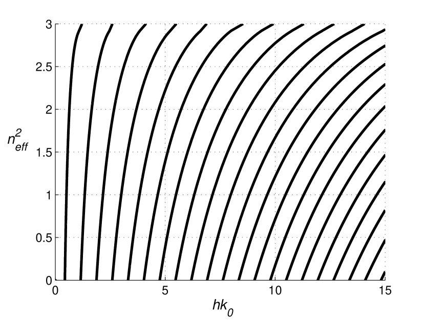
(c) $\kappa=0.85$

Figure 4: Dispersion curves for TM modes in case of $\varepsilon_{K}>0$, $\varepsilon_{e}<\varepsilon_{i}$. Mode marks are: (a) $m$ = 1, 2,…, 9, (b) $m$ = 1, 2,…, 12, (c) $m$ = 1, 2,…, 21.

In Fig. 4 dispersion curves for TM waves in case of $\varepsilon_{K}>0$ for different values of parameter $\kappa$ are presented. From the pictures follows that each TM mode also has two cutoff frequencies. But in comparison with self-defocusing case the dispersion curves density becomes higher with nonlinear parameter growth. And each curve shifts to the lower values of normalized core width or frequency. Thus in the focusing case a value of $n_{eff}^{2}$ increases with intensity at constant radiation frequency (or core width) finally achieves $\varepsilon_{e}$ value. Then considered mode leaves the waveguide.

Comparing the results obtained for cases $\varepsilon_{K}<0$ and $\varepsilon_{K}>0$ the first one seems to be more interesting: the number of possible solutions here decreases with intensity growth. This fact could prevent mode propagation from the inter-modes dispersion. And slowing light is possible.

In further parts of the paper we will analyze the case of slab waveguide with self-defocusing medium of the core in more details.

IV.1 The case of $\xi=1$

At maximum possible field intensity a nonlinear parameter $\xi$ is equal to value $\xi=1$. In this case the elliptic functions in the dispersion relation can be replaced by corresponding hyperbolic functions Batm:Erd:67 . Thus equation (16) is reduced to the form

$$\tanh\left(\frac{hk_{0}}{2\sqrt{2}}\sqrt{\varepsilon_{i}-n_{eff}^{2}}\right)\cosh^{2}\left(\frac{hk_{0}}{2\sqrt{2}}\sqrt{\varepsilon_{i}-n_{eff}^{2}}\right)=$$

$$\qquad\qquad=-\frac{\varepsilon_{i}}{\sqrt{|\varepsilon_{o}|\varepsilon_{e}}}\sqrt{\frac{\varepsilon_{e}-n_{eff}^{2}}{\varepsilon_{i}-n_{eff}^{2}}},$$ (19)

where a hyperbolic claddings with $\varepsilon_{o}<0$ and $\varepsilon_{e}>0$ was taken into account and the definitions of $p$, $q$ were used. As $hk_{0}\geq 0$ the relation (19) has solution only in following case

$$n_{eff}^{2}=\varepsilon_{e},~{}~{}hk_{0}=0.$$

But these conditions have no physical meaning (i.e., from this it follows that $h=0$).

V Influence of Field Energy Density on Mode Propagation Characteristics

This section is dedicated to analyze of the influence of propagating mode energy on the mode propagation characteristics, such as an effective refractive index and the cutoff frequencies in case $\varepsilon_{K}<0$.

In the previous sections a dimensionless parameter $\xi$ was used to account nonlinear effects in all principal equations describing guided wave. But $\xi$ has no clear physical meaning. So in the next analysis we will consider a carried density of energy $W$ as a parameter responsible for lever of nonlinearity influence.

The carried density of energy for planar wave in the dispersion-less medium can be obtained from the Brillouin formula for this case and takes a form:

$$W=\frac{1}{16\pi}\int_{-\infty}^{\infty}\left(\varepsilon_{e}|\tilde{E}_{x}|^{2}+\varepsilon_{o}|\tilde{E}_{z}|^{2}+|\tilde{H}_{y}|^{2}\right)dx,$$ (20)

where components of the TM wave field are defined by the equations (12) and (13). The dielectric constants $\varepsilon_{e}$, $\varepsilon_{o}$ are defined by (2).

V.1 Effective Refractive Index of the TM Modes

Let us consider a slab hyperbolic waveguide with fixed core width and guided TM wave with constant frequency defined by equality $hk_{0}=5$. Values of the linear dielectric constant are the same as were used in the previous section, $\varepsilon_{K}=-10^{-9}$ esu. In Fig. 5 ($a$) dispersion curves for linear case are presented. Dashed vertical line marks the value $hk_{0}=5$. From the picture follows that in the linear case modes with marks $m=2$ and $m=3$ can be exited in this waveguide. By comparing cases ($a$) ($b$) and ($c$) presented in the Fig.3 one can notice that with increasing of the nonlinear parameter $\xi$ the dispersion curves with marks $m=2$ and $m=3$ gradually leaves the waveguide. Also at certain value of $\xi$ the mode with $m=1$ can be exited in the waveguide while the modes with $m=2$ and $m=3$ can not be exited.

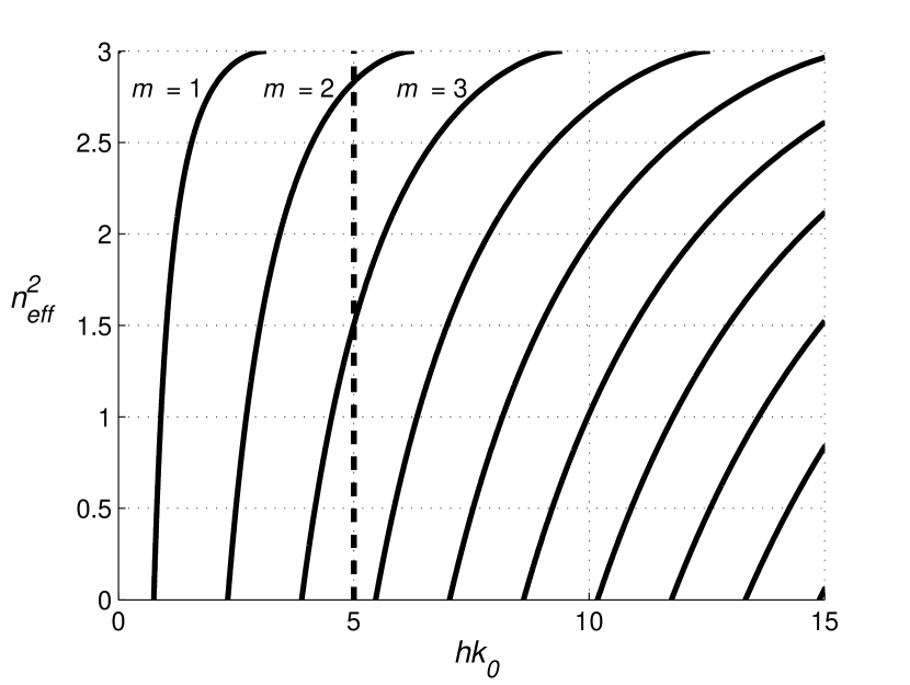
(a)

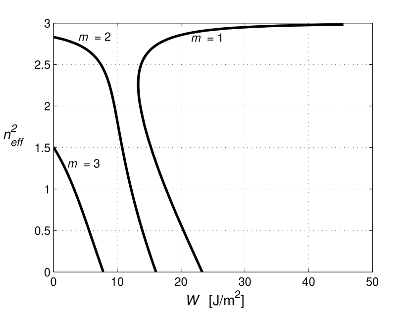
(b)

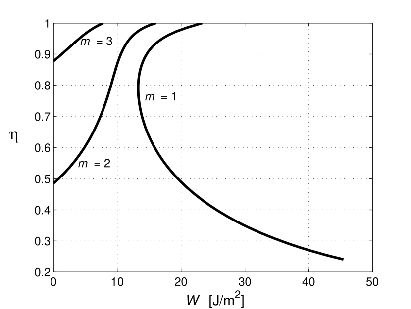
(c)

Figure 5: Hyperbolic waveguide with $hk_{0}=5$ ($a$) Dispersion curves for $\xi=0$; ($b$) Dependence of effective refractive index on carried density of energy; ($c$) Dependence of energy fraction in the core on carried density of energy.

An analogous behavior is illustrated in Fig. 5 ($b$). The picture shows how the square of effective indexes of possible modes varying with carried density of energy $W$. The core width and radiation frequency satisfy condition $hk_{0}=5$. All possible in this case mode marks are presented on the picture. At $W=0$ values of $n_{eff}^{2}$ for marks $m=2$ and $m=3$ are the same as in the linear case. They are also present in Fig. 5 ($a$) as intersections of dashed line with corresponding dispersion curves.

With increasing of carried density of energy $W$ values of $n_{eff}^{2}$ in cases $m=2$ and $m=3$ decrease more slowly at lower values of $W$ and faster at higher values. That is because dispersion curves presented in Fig.5 ($a$) or Fig.3, Fig.4 are more flat at higher $n_{eff}^{2}$ values. At certain value of $W$ mode with $m=3$ becomes stopped, i.e., the associated effective mode index $n_{eff}^{2}$ or propagation constant $\beta$ achieves zero value. After point $n_{eff}^{2}=0$ guided mode becomes decaying and not propagating. With further increasing of the electromagnetic field for mode with $m=2$ the propagation constant also becomes equal to zero.

The mode with mark $m=1$ presents a special situation. It does not exist in the linear case. But if $W$ exceeds a certain threshold value mode with $m=1$ appears in the waveguide. Another feature of this mode is that the function $n_{eff}^{2}(W)$ is double valued. One brunch of function has a similar behavior with cases $m=2$ and $m=3$: $n_{eff}^{2}$ decreases to zero value. At another brunch $n_{eff}^{2}$ tends to it maximum possible value $n_{eff}^{2}=\varepsilon_{e}$.

In Fig. 5 plot ($c$) shows the dependence of energy fraction $\eta$ to whole value $W$. The fraction $\eta$ is defined as

$$\eta=\frac{W_{core}}{W},$$

where $W_{core}$ is carried density of energy,which is concentrated in the waveguide core only. Comparing the figures ($b$) and ($c$) one can notice that with decreasing of $n_{eff}$ the guided wave becomes more confined in the waveguide. This fact will be considered in more details in the next subsection. If $n_{eff}^{2}$ tends to $\varepsilon_{e}$ the considered mode leaves the waveguide core. Two branches of the curve $m=1$ represent two guided modes. One of them corresponds to mode that is confined in the core, another one corresponds to mode with most of carrying energy concentrated in the waveguide claddings.

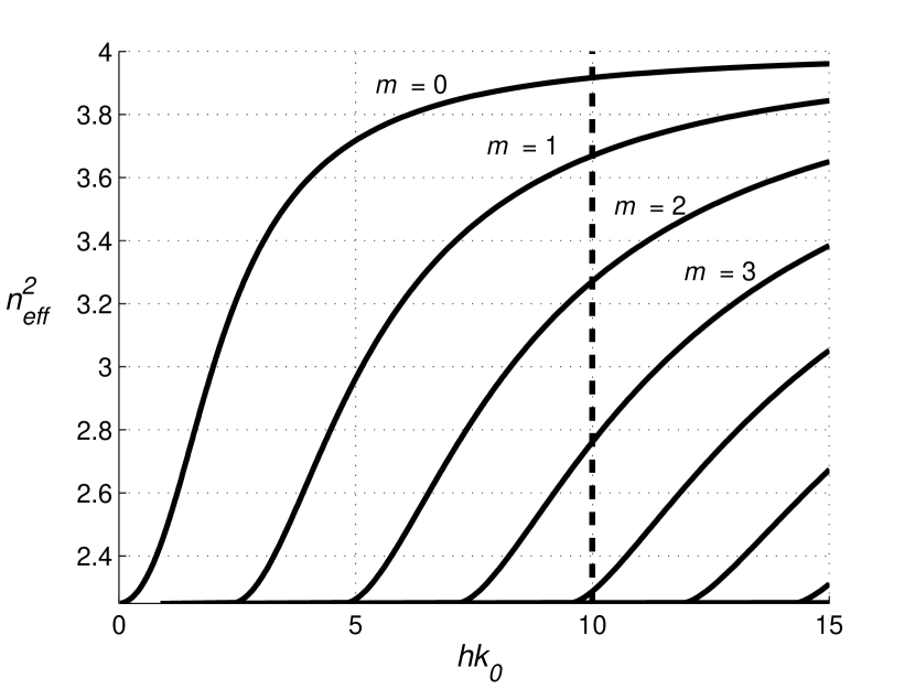
(a)

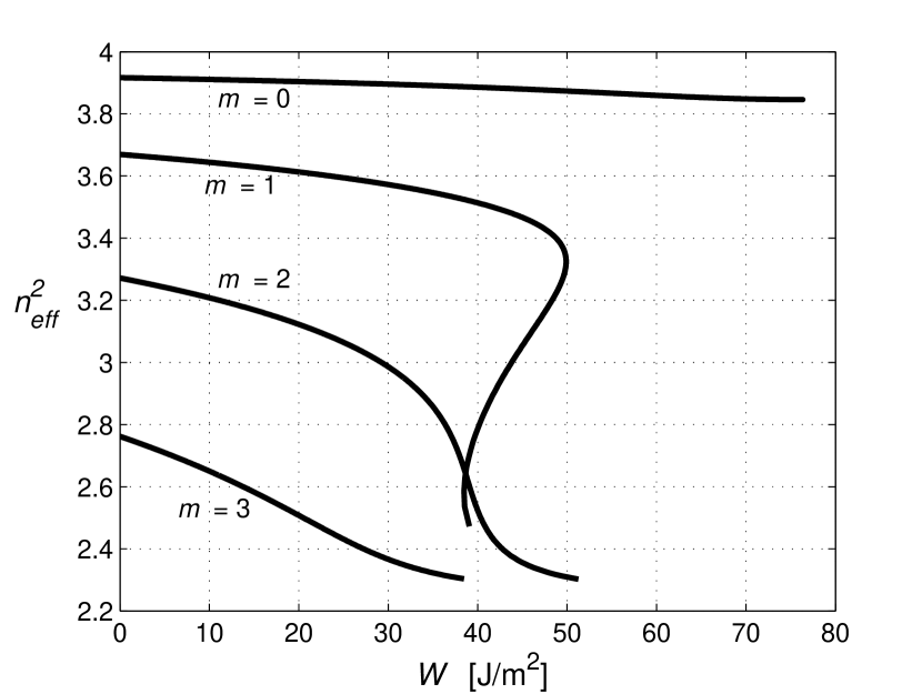
(b)

Figure 6: Usual dielectric waveguide with normalized core width $hk_{0}=10$. ($a$) Dispersion curves for $\xi=0$; ($b$) Dependence of effective refractive index on carried density of energy.

For comparison with obtained results the similar results for the usual dielectric slab waveguide with $\varepsilon_{i}=4.0$, $\varepsilon_{e}=\varepsilon_{o}=2.25$, $\varepsilon_{K}=-10^{-9}$ esu are presented in Fig.6. Normalized core width was proposed $hk_{0}=10$. In linear case modes with marks $m=0,1,\ldots,4$ can be exited. With increasing of the field intensity the linear values of $n_{eff}^{2}$ for each modes are decreased tending to theirs lowest values $n_{eff}^{2}=\varepsilon_{e}=\varepsilon_{o}$. No another curve appears. All possible mode are in the linear case already.

V.2 Decaying Length

Due to (12) a parameter $k_{\vec{n}}=iq$ is a projection of guided mode wave vector on normal direction to the waveguide layers. Thus $q$ is a constant that defines how far wave intensity can penetrate from the core to surrounding medium. Let us define a decaying length as

$$L_{d}=1/2q,$$

so at distance $L_{d}$ the field intensity $|E_{z}|^{2}$ decreases to $1/e$ of its previous value. As $n_{eff}$ depends on field carried density of energy $W$ the $L_{d}$ will also be changing with $W$.

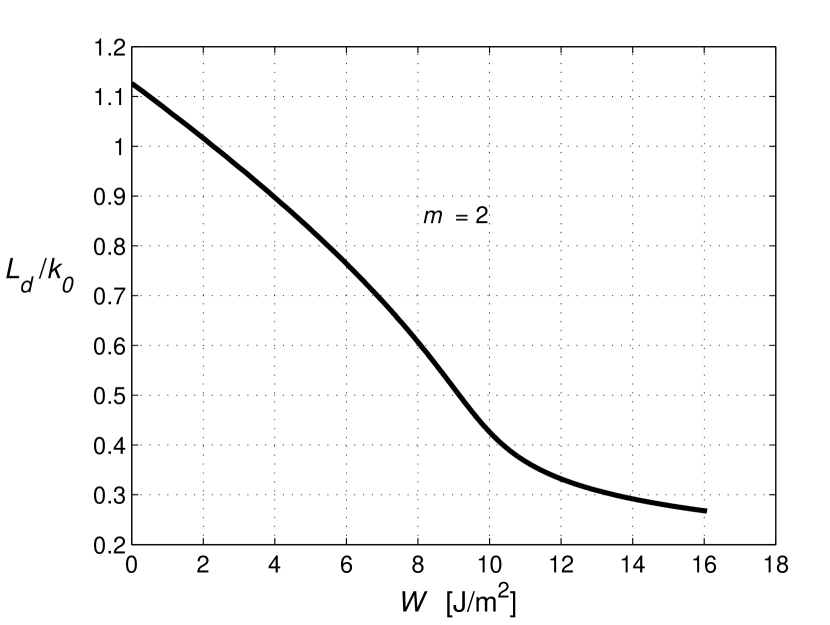
(a)

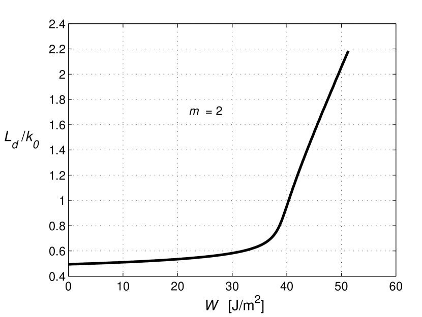
(b)

Figure 7: Dependence of decaying length in the claddings on surface density of energy. ($a$) Hyperbolic waveguide; ($b$) Usual dielectric waveguide.

The Fig.7 illustrates this dependence both for a hyperbolic waveguide ($a$) and a conventional waveguide case ($b$). The mode with mark $m=2$ was chosen for both pictures.

As was shown earlier, in case of self-defocusing Kerr-medium of the waveguide core the effective refractive index decreases with $W$. In the hyperbolic case the value of $q$ increases with $n_{eff}$ decaying. Parameter $q$ is inversely proportional to decay length $L_{d}$. Thus, the electromagnetic field will be more concentrated in the waveguide core. Width of the considered mode becomes more narrow with $W$. In the usual dielectric waveguide case at $\varepsilon_{o}>0$, $\varepsilon_{e}>0$ parameters $n_{eff}$ and $q$ are varying similarly. So with increasing of $W$ the electric field penetrates farther into the waveguide cladding.

In Fig.8 the field distributions for mode $m=2$ in the hyperbolic waveguide for lowest and highest values of $W$ are presented. Normalized waveguide core width is $hk_{0}=5$. Cases $(a)$ and $(c)$ correspond to $W\leq$ 1 J/m², $n_{eff}^{2}=2.28$. The cases $(b)$ and $(d)$ correspond to $W\geq 15$ J/m², $n_{eff}^{2}<0.05$. The distributions of the electric fields outside the core confirm the previous result presented in Fig. 7 ($a$).

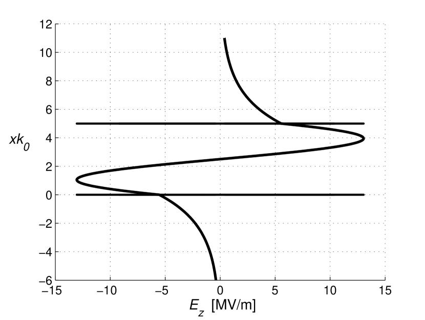
(a)

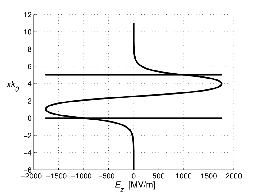
(b)

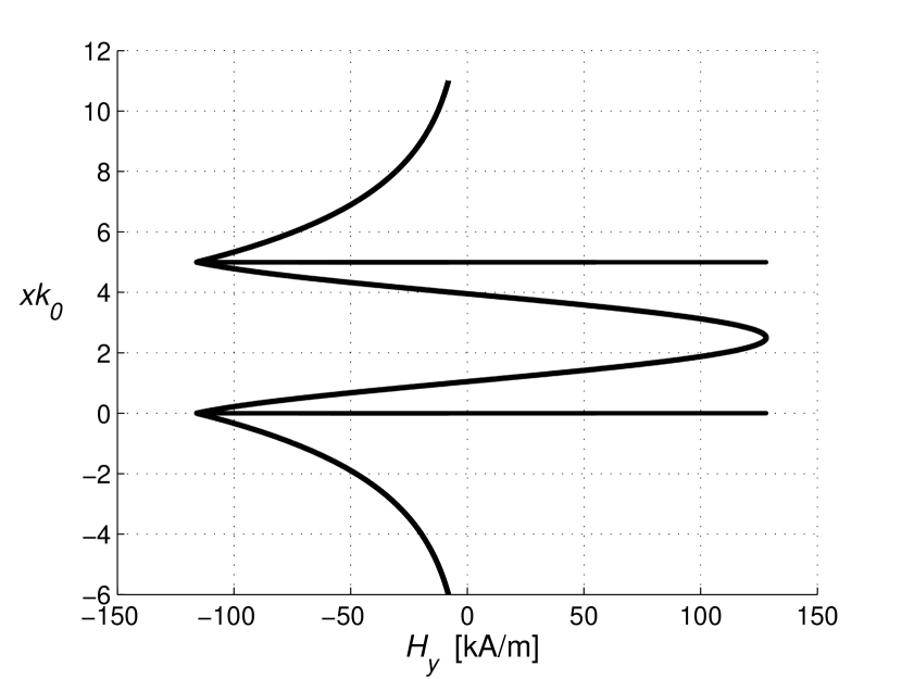
(c)

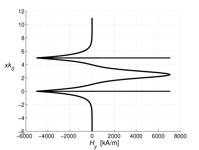
(d)

Figure 8: Field distributions in the hyperbolic waveguide for TM mode $m=2$. ($a$), ($b$) Electric field distributions at low and high intensity correspondingly; ($c$), ($d$) Magnetic field distributions at low and high intensity.

V.3 Cutoff Frequencies

It was shown earlier that each TM mode of the hyperbolic waveguide exists only in certain frequency range, i.e., there are two cutoff frequencies at $\varepsilon_{e}<\varepsilon_{i}$. In this subsection the influence of nonlinearity on cutoff frequencies of mode with index $m=2$ will be tested.

Let us define mode cutoff frequencies as

$$V_{cm}^{(1)}=hk_{0}(n_{eff}^{2}=0),~{}~{}~{}V_{cm}^{(2)}=hk_{0}(n_{eff}^{2}=\varepsilon_{e}),$$ (21)

where $m$ is a mode mark ($m=1,2,\ldots$) and the normalized frequency (or normalized width) $hk_{0}$ is solution of (16). So a slab hyperbolic waveguide with core width $h$ confines only TM mode for radiation frequencies lying in the corresponding interval

$$\frac{c}{h}V_{cm}^{(1)}\leq\omega\leq\frac{c}{h}V_{cm}^{(2)}.$$ (22)

Cutoff frequencies could be obtained from the equation (16) as functions of $\xi$ at appropriate values of parameters $p(n_{eff}^{2})$ and $q(n_{eff}^{2})$. The results for $m=2$ are presented in Fig.9 ($a$). Initial values of $V_{c2}^{(1)}$ and $V_{c2}^{(2)}$ at $\xi=0$ were defined from the linear dispersion equation obtained in Lyashko:15 . The influence of field carried density of energy on the cutoff frequencies are presented in Fig.9 ($b$). Dielectric constants are the same as in previous sections. Kerr constant was chosen to be equal to $\varepsilon_{K}=-10^{-9}$ esu.

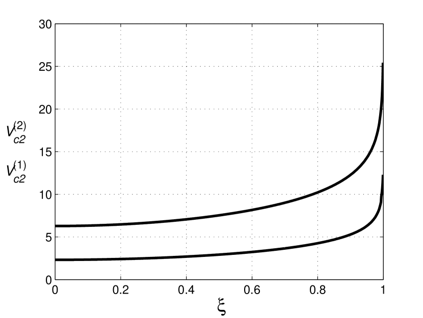
(a)

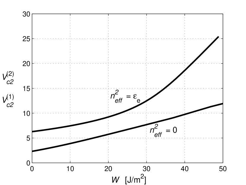
(b)

Figure 9: Dependence of cutoff frequencies on $\xi$ ($a$) and $W$ ($b$).

From the picture it follows that both cutoff frequencies increase with $\xi$ (intensity). The width of interval ($V_{cm}^{(1)}$, $V_{cm}^{(2)}$) slowly increase with $\xi$. At values $\xi\to 1$ both frequencies tend to infinity, that means that there are no guided waves in this waveguide.

Strictly speaking at limit value $\xi=1$ the following results for cutoff frequencies can be obtained

$$V_{cm}^{(1)}\to\infty,\quad V_{cm}^{(2)}=0.$$

Thus the function $V_{cm}^{(2)}(\xi)$ is continuous function in interval $[0,1)$.

VI Conclusion

Properties of the TM guided modes in the hyperbolic slab waveguide are theoretically investigated. The slab waveguide is formed from a non-dissipative dielectric core and a hyperbolic environment with anisotropy axis aligned with normal vector to the layers interfaces. The nonlinear Kerr response of the core was taken into account. Only evanescent waves are in the hyperbolic environment. So possible absorption of the hyperbolic medium was not considered. The effect of the dissipation has been discussed in LM:16 . As usually the losses lead to the guided wave amplitude decreasing. However, it was fond that if the carry wave frequency lies in transparency region of the hyperbolic medium the principal phenomena presented in the paper will exist and the effects of losses will be like effects in the case of waveguide with metallic covering layer.

The dispersion relation for the guided modes was found. It was shown that if dielectric constant of the core is greater then extraordinary permittivity of the environment each TM guided wave has two cutoff frequencies as well as in works Lyashko:15 ; LM:16 . So each mode can be exited only in appropriate frequency range. Contrary to the case considered in LM:16 , here the principal part of the guided wave energy in the waveguide with nonlinear core is localized in nonlinear dielectric medium. In the case of self-focusing Kerr medium of the core a number of possible modes increases with the field intensity. In case of self-defocusing medium this dependence is inverse.

The value of mode propagating constant decreases with intensity of the radiation field in the self-defocusing case. Hence the propagations constant will be zero at certain value of the intensity. With further increasing of field intensity mode becomes an evanescent and disappears. Thus varying the energy of the field one can obtain the slow-light waveguide of a new kind. The changing of a number of possible waveguide modes in the hyperbolic waveguide under consideration could be exploited to fabrication of the all-optical modulator or another all-optical devices.

The influence of carried density of energy on the mode width and cutoff frequencies was also analyzed in the self-defocusing core medium case. It was shown that with field energy growth mode width becomes more narrow as opposite to the usual dielectric waveguide case.

References

- (1) Elser J , Wangberg R , Podolskiy V A and Narimanov E E, 2006 Appl.Phys.Lett. 89 261102.
- (2) Noginov M A, Barnakov Yu A, Zhu G, Tumkur T, Li H, and Narimanov E E, 2009 Appl.Phys.Lett. 94 151105.
- (3) Poddubny Al N, Belov P A, Ginzburg P, Zayats A V, and Kivshar Yu S 2012 Phys.Rev. B 86 035148.
- (4) Poddubny Al, Belov P V, and Kivshar Yu S, 2013 Phys.Rev. A 87 035136.
- (5) Ferrari L., Dylan Lu, Lepage D , Zhaowei Liu, 2014 Opt. Express 22 4301–4306.
- (6) Benedicto J, Centeno E, Polles R, Moreau A, 2013 Phys.Rev. B 88 245138.
- (7) Zapata-Rodriguez C J, Miret J J, Vukovic S, Belic M R 2013 Opt. Express 21 19113 -19127.
- (8) Ni Xingjie, Ishii Satoshi, Thoreson M D, Shalaev Vl M, Seunghoon Han, Sangyoon Lee, and Kildishev Al V, 2011 Opt. Express 19 25242- 25254.
- (9) Drachev V P, Podolskiy V A, and Kildishev A V, 2013 Opt. Express 21 15048–15064.
- (10) Shekhar P, Atkinson J and Jacob Z, 2014 Nano Convergence 1:14 1–17.
- (11) Babicheva V E, Shalaginov M Y, Ishii S, Boltasseva A, and Kildishev Al V 2015 Opt. Express 23 31109–31119.
- (12) Babicheva V E, Shalaginov M Y, Ishii S, Boltasseva Al, and Kildishev Al V 2015 Opt. Express 23 9681–9689.
- (13) Y. J. Huang, W. T. Lu and S. Sridhar, 2008 Phys. Rev. A 77 063836.
- (14) Hua Zhu, Xiang Yin, Lin Chen, Zhongshu Zhu, and Xun Li, 2015 Opt. Lett. 40 4595–4598.
- (15) Guo-ding Xu, Tao Pan, Tao-cheng Zang and Jian Sun, 2008 Opt. Commun. 281 2819–2825.
- (16) Lyashko E I and Maimistov A I, 2015 Quantum Electronics 45 1050–1054.
- (17) Lyashko E I and Maimistov A I, 2016 J. Opt. Soc. Am. B 33 2320–2330.
- (18) Mihalache D, and Fedyanin V K, 1983 Teor. Mat. Fiz. 54 443–455 [1983 Theoretical and Mathematical Physics 54 289- 297 ]
- (19) Agranovich V M, Babichenko V S, and Chernyak V Ya, 1980 JETP Lett. 32 512–515.
- (20) Bateman H and Erdelyi A, (eds) 1955 Higer transcendntal functions vol 3 (New York, Toronto, London: Mc Graw-Hill Book Company).