Abstract

In this article we provide the Henon-Heiles system defined on Lie-algebraically deformed nonrelativistic space-time with the commutator of two spatial directions proportional to time. Particularly, we demonstrate that in such a model the total energy is not conserved and for this reason the role of control parameter is taken by the initial energy value $E_{0,{\rm tot}}=E_{{\rm tot}}(t=0)$. Besides, we show that in contrast with the commutative case, for chosen values of deformation parameter $\kappa$, there appears chaos in the system for initial total energies $E_{0,{\rm tot}}$ below the threshold $E_{0,{\rm th}}=1/6$.

1 Introduction

At the beginning of 70’s Edward Lorenz proposed his widely-known ”model of weather” containing the system of nonlinear and strongly sensitive with respect initial conditions differential equations [1]. Since this time there appears a lot of papers dealing with classical and quantum systems of which dynamic remains chaotic; the most popular of them are: Henon-Heiles system [2], Rayleigh-Bernard system [3], jerk equation [4], Duffing equation [5], double pendulum [6], [7], pendulum with forced damping [6], [7] and quantum forced damped oscillator model [8]. The first of them, so-called Henon-Heiles system, has been provided in pure astrophysical context, i.e., it concerns the problem of nonlinear motion of a star around of a galactic center where the motion is restricted to a plane. It is defined by the following Hamiltonian function

$$H(p,x)\;=\;\frac{1}{2}\sum_{i=1}^{2}\;\left(p_{i}^{2}+x_{i}^{2}\right)+x_{1}^{2}x_{2}-\frac{1}{3}x_{2}^{3}\;,$$ (1)

which in cartesian coordinates $x_{1}$ and $x_{2}$ describes the set of two nonlinearly coupled harmonic oscillators. In polar coordinates $r$ and $\theta$ it corresponds to the particle moving in noncentral potential of the form

$$V(r,\varphi)\;=\;\frac{r^{2}}{2}+\frac{r^{3}}{3}\sin\left(3\varphi\right)\;,$$ (2)

with $x_{1}=r\cos\varphi$ and $x_{2}=r\sin\varphi$. The above model has been inspired by observations indicating that star moving in a weakly perturbated central potential should has apart of total energy $E_{\rm{tot}}$ constant in time also the second conserved physical quantity $I$. It has been demonstrated with use of so-called Poincare section method, that such a situation appears in the case of Henon-Heiles system only for the values of control parameter $E_{\rm{tot}}$ below the threshold $E_{\rm th}=1/6$. For higher energies the trajectories in phase space become chaotic and the quantity $I$ does not exist (see e.g. [9], [10]).

Our aim in this paper is to study further the impact of noncommutative generalization of the model on its chaotic properties. Recently, there has been proposed in article [11] the noncommutative counterpart of Henon-Heiles system defined on the following canonically deformed Galilei space-time [12]-[14],

$$[\;t,\hat{x}_{i}\;]=0\;\;\;,\;\;\;[\;\hat{x}_{i},\hat{x}_{j}\;]=i\theta_{ij}\;,$$ (3)

with $\theta_{ij}=-\theta_{ji}={\rm const.}$ Particularly, there has been provided the Hamiltonian function of the model as well as the corresponding canonical equations of motion. Besides, it has been demonstrated that for proper values of deformation parameter $\theta$ and for proper values of control parameter $E_{\rm{tot}}$ there appears (much more intensively) chaos in the system. Consequently, in such a way it has been shown the impact of most simple space-time noncommutativity on the basic dynamical properties of this important classical chaotic model. It should be noted, however, that there exist a lot of papers dealing with noncommutative classical and quantum mechanics (see e.g. [22]-[25]) as well as with field theoretical systems (see e.g. [26]-[28]), in which the quantum space-time is not classical. Such models follow, in particular, from formal arguments based mainly on Quantum Gravity [29], [30] and String Theory [31], [32] indicating that space-time at Planck scale becomes noncommutative.

In present article we provide another noncommutative Henon-Heiles system defined on the following Lie-algebraically deformed space-time [14]

$$[\;t,\hat{x}_{i}\;]=0\;\;\;,\;\;\;[\;\hat{x}_{i},\hat{x}_{j}\;]=\frac{i}{\kappa}t\epsilon_{ij}\;,$$ (4)

with deformation parameter $\kappa$. In such a way we get the model with time-dependent Hamiltonian function in which the role of control parameter is taken over by the initial value of total energy $E_{0,\rm{tot}}=E_{\rm{tot}}(t=0)$. We shall demonstrate with use of Poincare section method, that contrary to the commutative case, there appears for suitable values of deformation parameter $\kappa$ chaos below the threshold $E_{0,\rm{th}}=1/6$. We interpret such a result as an effect of the time dependence of Hamiltonian function of the model.

The paper is organized as follows. In second Section we briefly remind the basic properties of classical Henon-Heiles system. In Section 3 we recall Lie-algebraic noncommutative quantum Galilei space-time proposed in article [14]. Section 4 is devoted to the new Lie-algebraically deformed Henon-Heiles model while the conclusions are discussed in Sect. 5, describing final remarks.

2 Classical Henon-Heiles model

As it was already mentioned the Henon-Heiles system is defined by the following Hamiltonian function

$$H(p,x)\;=\;\frac{1}{2}\sum_{i=1}^{2}\;\left(p_{i}^{2}+x_{i}^{2}\right)+x_{1}^{2}x_{2}-\frac{1}{3}x_{2}^{3}\;,$$ (5)

with canonical variables $(p_{i},x_{i})$ satisfying

$$\{\;x_{i},x_{j}\;\}=0=\{\;p_{i},p_{j}\;\}\;\;\;,\;\;\;\{\;x_{i},p_{j}\;\}=\delta_{ij}\;,$$ (6)

i.e., it describes the system of two nonlineary coupled one-dimensional harmonic oscillator models. One can check that the corresponding canonical equations of motion take the form

$$\dot{p}_{1}\;=\;-\frac{\partial H}{\partial x_{1}}\;=\;-x_{1}-2x_{1}x_{2}\;\;\;,\;\;\;\dot{x}_{i}\;=\;\frac{\partial H}{\partial p_{i}}\;=\;p_{i}\;,$$ (7)

$$\dot{p}_{2}\;=\;-\frac{\partial H}{\partial x_{2}}\;=\;-x_{2}-x_{1}^{2}+x_{2}^{2}\;,$$ (8)

while the proper Newton equations look as follows

$$\left\{\begin{array}[]{rcl}\ddot{x}_{1}&=&-x_{1}-2x_{1}x_{2}\\[5.0pt] \ddot{x}_{2}&=&-x_{2}-x_{1}^{2}+x_{2}^{2}\;.\end{array}\right.$$ (9)

Besides, it is easy to see that the conserved in time total energy of the model is given by

$$E_{\rm tot}\;=\;\frac{1}{2}\sum_{i=1}^{2}\;\left(\dot{x}_{i}^{2}+x_{i}^{2}\right)+x_{1}^{2}x_{2}-\frac{1}{3}x_{2}^{3}\;.$$ (10)

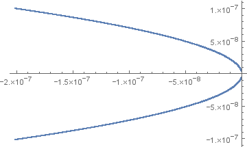
Figure 1: Poincare map in two dimensional phase space $(x_{2},p_{2})$ for section $x_{1}=0$ and for total energy $E_{\rm tot}=0.00000015$ lying down below the threshold $E_{\rm th}=1/6$. Trajectory is completely regular - there is no chaos in the system.

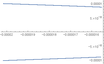
Figure 2: Poincare map in two dimensional phase space $(x_{2},p_{2})$ for section $x_{1}=0$ and for total energy $E_{\rm tot}=0.000015$ lying down below the threshold $E_{\rm th}=1/6$. Trajectory is completely regular - there is no chaos in the system.

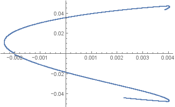
Figure 3: Poincare map in two dimensional phase space $(x_{2},p_{2})$ for section $x_{1}=0$ and for total energy $E_{\rm tot}=0.0015125$ lying down below the threshold $E_{\rm th}=1/6$. Trajectory is completely regular - there is no chaos in the system.

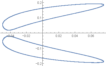
Figure 4: Poincare map in two dimensional phase space $(x_{2},p_{2})$ for section $x_{1}=0$ and for total energy $E_{\rm tot}=0.03125$ lying down below the threshold $E_{\rm th}=1/6$. Trajectory is completely regular - there is no chaos in the system.

In order to illustrate the basic properties of discussed system we find numerically the Poincare maps in two dimensional phase space $(x_{2},p_{2})$ for section $x_{1}=0$ and for four fixed values of total energy $E_{\rm{tot}}$ below the threshold $E_{\rm th}=1/6$: $E_{\rm tot}=0.00000015$, $E_{\rm tot}=0.000015$, $E_{\rm tot}=0.0015125$ and $E_{\rm tot}=0.03125$; the obtained results are summarized on Figures 1 - 4 respectively. Consequently, one can see that in such a case the all trajectories (in fact) remain completely regular.

3 Lie-algebraically deformed Galilei space-time

In this section we very shortly recall the basic facts associated with the (twisted) canonically deformed Galilei Hopf algebra $\;{\cal U}_{\kappa}({\cal G})$ and with the corresponding quantum space-time [14]. First of all, it should be noted that in accordance with Drinfeld twist procedure [33] the algebraic sector of Hopf structure $\;{\cal U}_{\kappa}({\cal G})$ remains undeformed

$$\left[\,K_{ij},K_{kl}\,\right]=i\left(\delta_{il}\,K_{jk}-\delta_{jl}\,K_{ik}+\delta_{jk}K_{il}-\delta_{ik}K_{jl}\right)\;,$$ (11)

(13)

$$\left[\,K_{ij},V_{k}\,\right]=i\left(\delta_{jk}\,V_{i}-\delta_{ik}\,V_{j}\right)\;\;\;,\;\;\;\left[\,K_{ij},\Pi_{\rho}\right]=i\left(\eta_{j\rho}\,\Pi_{i}-\eta_{i\rho}\,\Pi_{j}\right)\;,$$

(15)

$$\left[\,V_{i},V_{j}\,\right]=\left[\,V_{i},\Pi_{j}\,\right]=0\;\;\;,\;\;\;\left[\,V_{i},\Pi_{0}\,\right]=-i\Pi_{i}\;\;\;,\;\;\;\left[\,\Pi_{\rho},\Pi_{\sigma}\,\right]=0\;,$$

where $K_{ij}$, $\Pi_{0}$, $\Pi_{i}$ and $V_{i}$ can be identified with rotation, time translation, momentum and boost operators respectively. Besides, the coproducts and antipodes of such algebra take the form

$$\Delta_{{\kappa}}(\Pi_{0}) = \Delta_{0}(\Pi_{0})+\frac{1}{2{{\kappa}}}\Pi_{l}\wedge\Pi_{k}\;,$$ (16)

(17)

$$\Delta_{{\kappa}}(\Pi_{i}) = \Delta_{0}(\Pi_{i})\;\;\;,\;\;\;\Delta_{{\kappa}}(V_{i})=\Delta_{0}(V_{i})\;,$$ (18)

(19)

$$\Delta_{{\kappa}}(K_{ij}) = \Delta_{0}(K_{ij})+\frac{i}{2{{\kappa}}}\left[\,K_{ij},V_{k}\,\right]\wedge\Pi_{l}\;+$$ (20)

$$~{}~{}~{}~{}~{}~{}~{}~{}~{}~{}~{}~{}~{}~{}~{}~{}~{}~{}~{}~{}~{}~{}~{}~{}~{}~{}+\;\frac{1}{2{{\kappa}}}V_{k}\wedge(\delta_{il}\Pi_{j}-\delta_{jl}\Pi_{i})\;,$$

while the corresponding quantum space-time can be defined as the representation space, so-called Hopf modules (see e.g. [12], [13]), for the Lie-algebraically deformed Hopf structure $\;{\cal U}_{\kappa}({\cal G})$; it looks as follows

$$[\;t,\hat{x}_{i}\;]=0\;\;\;,\;\;\;[\;\hat{x}_{i},\hat{x}_{j}\;]=i\frac{t}{\kappa}(\delta_{li}\delta_{kj}-\delta_{ki}\delta_{lj})\;,$$ (22)

and for deformation parameter $\kappa$ approaching infinity it becomes commutative.

4 Lie-algebraically deformed classical Henon-Heiles system

Let us now turn to the Henon-Heiles model defined on quantum space-time (4). In first step of our construction we extend the Lie-algebraically deformed space to the whole algebra of momentum and position operators as follows (see e.g. [34]-[36])

$$\{\;\hat{x}_{1},\hat{x}_{2}\;\}=\frac{2t}{\kappa}\;\;\;,\;\;\;\{\;\hat{p}_{i},\hat{p}_{j}\;\}=0\;\;\;,\;\;\;\{\;\hat{x}_{i},\hat{p}_{j}\;\}=\delta_{ij}\;.$$ (23)

One can check that relations (23) satisfy the Jacobi identity and for deformation parameter $\kappa$ approaching infinity become classical.
Next, by analogy to the commutative case we define the corresponding Hamiltonian function by

$$H(\hat{p},\hat{x})\;=\;\frac{1}{2}\sum_{i=1}^{2}\;\left(\hat{p}_{i}^{2}+\hat{x}_{i}^{2}\right)+\hat{x}_{1}^{2}\hat{x}_{2}-\frac{1}{3}\hat{x}_{2}^{3}\;,$$ (24)

with the noncommutative operators $({\hat{x}}_{i},{\hat{p}}_{i})$ represented by the classical ones $({x}_{i},{p}_{i})$ as [36]-[38]

$${\hat{x}}_{1} = {x}_{1}-{\frac{t}{\kappa}}p_{2}\;,$$ (25)

$${\hat{x}}_{2} = {x}_{2}+{\frac{t}{\kappa}}p_{1}\;,$$ (26)

$${\hat{p}}_{1} = {p}_{1}\;\;,\;\;{\hat{p}}_{2}\;=\;{p}_{2}\;.$$ (27)

Consequently, we have

$$H({p},{x},t) = \frac{1}{2M\left(\frac{t}{\kappa}\right)}\left({{{p}}_{1}^{2}}+{{{p}}_{2}^{2}}\right)+\frac{1}{2}M\left(\frac{t}{\kappa}\right)\Omega^{2}\left(\frac{t}{\kappa}\right)\left({{{x}}_{1}^{2}}+{{{x}}_{2}^{2}}\right)-S\left(\frac{t}{\kappa}\right)L\;+$$

$$+ \left(x_{1}-{\frac{t}{\kappa}p_{2}}\right)^{2}\left(x_{2}+{\frac{t}{\kappa}p_{1}}\right)-\frac{1}{3}\left(x_{2}+{\frac{t}{\kappa}p_{1}}\right)^{3}\;,$$

where

$$L=x_{1}p_{2}-x_{2}p_{1}\;,$$ (29)

$$\frac{1}{M\left(\frac{t}{\kappa}\right)}=1+\left(\frac{t}{\kappa}\right)^{2}\;,$$ (30)

$$\Omega\left(\frac{t}{\kappa}\right)=\sqrt{\left(1+\left(\frac{t}{\kappa}\right)^{2}\right)}\;,$$ (31)

and

$$S\left(\frac{t}{\kappa}\right)=\frac{t}{\kappa}\;.$$ (32)

We see that the Hamiltonian function depends on time and for this reason the role of control parameter in the model is taken by initial value of total energy $E_{0,{\rm tot}}=E_{\rm tot}(t=0)$. Besides, using the formula (4) one gets the following canonical equations of motion

$$\left\{\begin{array}[]{rcl}\dot{x}_{1}&=&\frac{1}{M\left(\frac{t}{\kappa}\right)}p_{1}+S\left(\frac{t}{\kappa}\right)x_{2}+\left[\left(x_{1}-\frac{t}{\kappa}p_{2}\right)^{2}-\left(x_{2}+\frac{t}{\kappa}p_{1}\right)^{2}\right]\frac{t}{\kappa}\\[5.0pt] &{}{}\hfil&{}\cr\dot{x}_{2}&=&\frac{1}{M\left(\frac{t}{\kappa}\right)}p_{2}-S\left(\frac{t}{\kappa}\right)x_{1}-2\left[x_{2}+\frac{t}{\kappa}p_{1}\right]\left[x_{1}-\frac{t}{\kappa}p_{2}\right]\frac{t}{\kappa}\\[5.0pt] &{}{}\hfil&{}\cr\dot{p}_{1}&=&-{M\left(\frac{t}{\kappa}\right)}\Omega^{2}\left(\frac{t}{\kappa}\right)x_{1}+S\left(\frac{t}{\kappa}\right)p_{2}-2\left[x_{2}+\frac{t}{\kappa}p_{1}\right]\left[x_{1}-\frac{t}{\kappa}p_{2}\right]\\[5.0pt] &{}{}\hfil&{}\cr\dot{p}_{2}&=&-{M\left(\frac{t}{\kappa}\right)}\Omega^{2}\left(\frac{t}{\kappa}\right)x_{2}-S\left(\frac{t}{\kappa}\right)p_{1}-\left[x_{1}-\frac{t}{\kappa}p_{2}\right]^{2}+\left[x_{2}+\frac{t}{\kappa}p_{2}\right]^{2}\;,\end{array}\right.$$ (33)

which for deformation parameter running to infinity become classical.

Similarly to the undeformed case we find numerically the Poincare maps in two dimensional phase space $(x_{2},p_{2})$ for section $x_{1}=0$. We perform our calculations for exactly the same initial values of total energy as in commutative model, however, this time, apart of parameter $E_{0,{\rm tot}}$ we take under consideration the parameter of deformation $\kappa$. Consequently, we derive the Poincare sections of phase space for four pairs: $\left(E_{0,{\rm tot}}=0.00000015,1/\kappa=0.0001\right)$, $\left(E_{0,{\rm tot}}=0.000015,1/\kappa=0.001\right)$, $(E_{0,{\rm tot}}=0.0015125,$ $1/\kappa=0.001)$ and $\left(E_{0,{\rm tot}}=0.03125,1/\kappa=0.0001\right)$, and we represent them on Figures 5 - 8 respectively. In such a way we demonstrate that contrary to the undeformed Henon-Heiles system there appears chaos in the model for initial energies $E_{0,\rm{tot}}$ below the threshold $E_{0,{\rm th}}=1/6$.

5 Final remarks

In this article we provide the Henon-Heiles system defined on Lie-algebraically deformed nonrelativistic space-time with the commutator of two spatial directions proportional to time. Particularly, we demonstrate that in such a model the total energy is not conserved and for this reason the role of control parameter is taken by the initial energy value $E_{0,{\rm tot}}=E_{{\rm tot}}(t=0)$. Besides, we show that in contrast with the commutative case, for chosen values of deformation parameter $\kappa$, there appears chaos in the system for initial total energies $E_{0,{\rm tot}}$ below the threshold $E_{0,{\rm th}}=1/6$.

It should be noted that the present studies can be extended in various ways. First of all one may consider more complicated noncommutative Henon-Heiles models defined, for example, on the quadratic space-times provided in article [14]. Besides, it is possible to investigate the Lie-algebraic deformation of so-called generalized Henon-Heiles systems given by the following Hamiltonian function

$$H(p,x)\;=\;\frac{1}{2}\left(p_{1}^{2}+p_{2}^{2}\right)+\delta x_{1}^{2}+(\delta+\Omega)x_{2}^{2}+\alpha x_{1}^{2}x_{2}+\alpha\beta x_{2}^{3}\;,$$ (34)

with arbitrary coefficients $\alpha$, $\beta$, $\delta$ and $\Omega$ respectively. It should be noted that the properties of commutative models described by function (34) are quite interesting. For example, it is well-known (see e.g. [39]-[42] and references therein) that such systems remain integrable only in the Sawada-Kotera case: with $\beta=1/3$ and $\Omega=0$, in the KdV case: with $\beta=2$ and arbitrary $\Omega$ as well as in the Kaup-Kupershmidt case: with $\beta=16/3$ and $\Omega=15\delta$. Besides, there has been provided in articles [43] and [44] the different types of integrable perturbations of mentioned above (integrable) models such as, for example, $q^{-2}$ perturbations, the Ramani series of polynomial deformations and the rational perturbations. Consequently, the impact of the Lie-algebraic deformation (4) on the above dynamical structures (in fact) seems to be very interesting. For this reason the works in this direction already started and are in progress.

                  

                  

                  

                  

                  

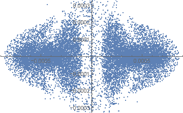
Figure 5: Poincare map in two dimensional phase space $(x_{2},p_{2})$ for section $x_{1}=0$ and for deformation parameter $1/\kappa=0.0001$ as well as for initial value of total energy $E_{0,{\rm tot}}=0.00000015$ lying down below the threshold $E_{0,{\rm th}}=1/6$. Trajectory is partially chaotic.

                  

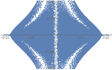
Figure 6: Poincare map in two dimensional phase space $(x_{2},p_{2})$ for section $x_{1}=0$ and for deformation parameter $1/\kappa=0.001$ as well as for initial value of total energy $E_{0,{\rm tot}}=0.000015$ lying down below the threshold $E_{0,{\rm th}}=1/6$. Trajectory is almost completely chaotic.

                  

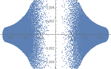
Figure 7: Poincare map in two dimensional phase space $(x_{2},p_{2})$ for section $x_{1}=0$ and for deformation parameter $1/\kappa=0.001$ as well as for initial value of total energy $E_{0,{\rm tot}}=0.0015125$ lying down below the threshold $E_{0,{\rm th}}=1/6$. Trajectory is partially chaotic.

                  

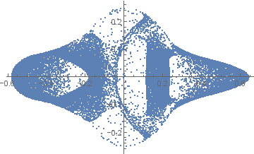
Figure 8: Poincare map in two dimensional phase space $(x_{2},p_{2})$ for section $x_{1}=0$ and for deformation parameter $1/\kappa=0.0001$ as well as for initial value of total energy $E_{0,{\rm tot}}=0.03125$ lying down below the threshold $E_{0,{\rm th}}=1/6$. Trajectory is partially chaotic.

References

• [1] E.N. Lorenz, J. Atmos. Sci. 20, 130 (1963)
• [2] M. Henon, C. Heiles, AJ. 69, 73 (1964)
• [3] S. Chandrasekhar, ”Hydrodynamic and Hydromagnetic Stability” (Dover), ISBN 0-486-64071-X, 1982.
• [4] J.C. Sprott, Am J Phys. 65, 537 (1997)
• [5] G. Duffing, ”Erzwungene Schwingungen bei Ver nderlicher Eigenfrequenz”, F. Vieweg u. Sohn, Braunschweig, 1918.
• [6] D.A. Wells, ”Theory and Problems of Lagrangian Dynamics”, New York: McGraw-Hill, pp. 13-14, 24, and 320-321, 1967.
• [7] V.I. Arnold, ”Problem in Mathematical Methods of Classical Mechanics”, 2nd ed. New York: Springer-Verlag, p. 109, 1989.
• [8] W.P. Schleich, ”Quantum Optics in Phase Space”, WILEY VCH, Berlin, 2001.
• [9] M. Tabor, ”Chaos and integrability in nonlinear dynamics”, New York: Wiley, 1989.
• [10] M.C. Gutzwiller, ”Chaos in Classical and Quantum Mechanics”, Springer-Verlag, Berlin, 1989.
• [11] M. Daszkiewicz, Acta Phys. Polon. B 47, 2387 (2016); arXiv: 1610.08361 [physics.class-ph]
• [12] R. Oeckl, J. Math. Phys. 40, 3588 (1999)
• [13] M. Chaichian, P.P. Kulish, K. Nashijima, A. Tureanu, Phys. Lett. B 604, 98 (2004); hep-th/0408069
• [14] M. Daszkiewicz, Mod. Phys. Lett. A 23, 505 (2008); arXiv: 0801.1206 [hep-th]
• [15] S. Zakrzewski, ”Poisson Structures on the Poincare group”; q-alg/9602001
• [16] Y. Brihaye, E. Kowalczyk, P. Maslanka, ”Poisson-Lie structure on Galilei group”; math/0006167
• [17] J. Lukierski, A. Nowicki, H. Ruegg and V.N. Tolstoy, Phys. Lett. B 264, 331 (1991)
• [18] S. Giller, P. Kosinski, M. Majewski, P. Maslanka and J. Kunz, Phys. Lett. B 286, 57 (1992)
• [19] J. Lukierski and M. Woronowicz, Phys. Lett. B 633, 116 (2006); hep-th/0508083
• [20] O. Ogievetsky, W.B. Schmidke, J. Wess, B. Zumino, Comm. Math. Phys. 150, 495 (1992)
• [21] P. Aschieri, L. Castellani, A.M. Scarfone, Eur. Phys. J. C 7, 159 (1999); q-alg/9709032
• [22] A. Deriglazov, JHEP 0303, 021 (2003); hep-th/0211105
• [23] S. Ghosh, Phys. Lett. B 648, 262 (2007)
• [24] M. Chaichian, M.M. Sheikh-Jabbari, A. Tureanu, Phys. Rev. Lett. 86, 2716 (2001); hep-th/0010175
• [25] Kh.P. Gnatenko, V.M. Tkachuk, Phys. Lett. A 378, 3509 (2014); arXiv: 1407.6495 [quant-ph]
• [26] P. Kosinski, J. Lukierski, P. Maslanka, Phys. Rev. D 62, 025004 (2000); hep-th/9902037
• [27] M. Chaichian, P. Prešnajder and A. Tureanu, Phys. Rev. Lett. 94, 151602 (2005); hep-th/0409096
• [28] G. Fiore, J. Wess, Phys. Rev. D 75, 105022 (2007); hep-th/0701078
• [29] S. Doplicher, K. Fredenhagen, J.E. Roberts, Phys. Lett. B 331, 39 (1994); Comm. Math. Phys. 172, 187 (1995); hep-th/0303037
• [30] A. Kempf and G. Mangano, Phys. Rev. D 55, 7909 (1997); hep-th/9612084
• [31] A. Connes, M.R. Douglas, A. Schwarz, JHEP 9802, 003 (1998); hep-th/9711162
• [32] N. Seiberg and E. Witten, JHEP 9909, 032 (1999); hep-th/9908142
• [33] V.G. Drinfeld, Soviet Math. Dokl. 32, 254-258 (1985); Algebra i Analiz (in Russian), 1, Fasc. 6, p. 114 (1989)
• [34] M. Chaichian, M.M. Sheikh-Jabbari, A. Tureanu, Eur. Phys. J. C 36 (2004) 251; hep-th/0212259
• [35] S. Gangopadhyay, A. Saha, A. Halder, Phys. Lett. A 379 (2015) 2956; arXiv: 1412.3581 [hep-th]
• [36] J.M. Romero, J.A. Santiago, J.D. Vergara, Phys. Lett. A 310, 9 (2003); hep-th/0211165
• [37] Y. Miao, X. Wang, S. Yu, Annals Phys. 326, 2091 (2011); arXiv: 0911.5227 [math-ph]
• [38] A. Kijanka, P. Kosinski, Phys. Rev. D 70, 12702 (2004); hep-th/0407246
• [39] T. Bountis, H. Segur, F. Vivaldi, Phys. Rev. A 25, 1257 (1982)
• [40] Y.F. Chang, M. Tabor, J. Weiss, J. Math. Phys. 23, 531 (1982)
• [41] S. Wojciechowski, Phys. Lett. A 100, 277 (1984)
• [42] A.P. Fordy, Physica D 52, 204 (1990)
• [43] A. Ballesteros, A. Blasco, Annals of Physics 325, 2787 (2010); arXiv: 1011.3005 [math-ph]
• [44] A. Ballesteros, A. Blasco, F.J. Herranz, J. Phys: Conf. Ser. 597 (2015) 012013; arXiv: 1503.09187 [nlin.SI]
Refer to caption