Error identities for variational problems with obstacles

Abstract.

The paper is concerned with a class of nonlinear free boundary problems, which are usually solved by variational methods based on primal (or primal–dual) variational settings. We deduce and investigate special relations (error identities). They show that a certain nonlinear measure of the distance to the exact solution (specific for each problem) is equivalent to the respective duality gap, which minimization is a keystone of all variational numerical methods. Therefore, the identity defines the measure that contains maximal quantitative information on the quality of a numerical solution available through these methods. The measure has quadratic terms generated by the linear part of the differential operator and nonlinear terms associated with free boundaries. We obtain fully computable two sided bounds of this measure and show that they provide efficient estimates of the distance between the minimizer and any function from the corresponding energy space. Several examples show that for different minimization sequence the balance between different components of the overall error measure may be different and domination of nonlinear terms may indicate that coincidence sets are approximated incorrectly.

1. Introduction

Variational inequalities form an important class of nonlinear models that describe free boundary phenomena arising in various applied problems (see, e.g., G. Duvaut and J. L. Lions [8] and other publications cited therein). Usually free boundaries separate regions where solutions possess quite different physical properties. Therefore, any reliable information on the shape and location of such a boundary is very important. Qualitative properties of free boundaries are studied by purely analytical (a priori) methods unlike quantitative information, which in the vast majority of cases can be obtained only by computational methods. In this context, it is necessary to know which quantitative information could be indeed extracted from a numerical solution.

In this paper, we are concerned with two classes of variational inequalities generated by obstacle type conditions. Differentiability properties of exact solutions to these problems are, in general, restricted even if all external data of a problem are smooth (e.g., see the works of H. Brezis [1], L.A. Caffarelli [7], D. Kinderlehrer and G. Stampacchia [16], A. Friedman [10], N. N. Uraltseva [28]). In [2] it was proved that there exists a unique solution $u\in W^{2,2}(\Omega)$ of an obstacle problem

$$\int\limits_{\Omega}\nabla u\cdot\nabla wdx\,\geq\,\int\limits_{\Omega}fw\,dx\;\;\;\forall w\in K:=\{w\in H^{1}(\Omega)\,\mid\,w=u_{D}\,on\,\partial\Omega,\,\,w\geq\psi\}$$

if $\psi\in W^{2,2}(\Omega)$, $f\in L^{2}$, the function $u_{D}$ (which defines the Dirichlét boundary condition) belongs to $W^{2,2}(\Omega)$ and satisfies the natural condition $u_{D}\geq\psi$ on $\partial\Omega$.

Many researches were focused on clarifying mathematical properties of the coincidence set. In particular, it was proved that if the domain $\Omega\subset R^{2}$ is strictly convex with a smooth boundary $\partial\Omega$ and if the obstacle $\psi\in C^{2}(\Omega)$ is strictly concave, then the coincidence set is connected and its boundary is smooth and homeomorphic to the unit circle (see, e.g. [16]). However, in general, the structure of a coincidence set can be very complicated and for any domain one can point out such an obstacle that this set has any number of disjoint subsets.

Numerical methods for problems with obstacles (and many other problems related to variational inequalities) were systematically studied in R. Glowinski, J.-L. Lions, and R. Tremolieres [12, 11]. Getting the respective a priori rate convergence estimates (in terms of the mesh size $h$) was the first question studied by many authors. In the context of finite element approximations such type estimates were derived by R. S. Falk [9] who proved the standard a priori convergence error estimates (with the rate $h$ for the $L^{2}$ norm of gradients and the rate $h^{2}$ for the $L^{2}$ norm of the functions) provided that $u\in W^{2,2}$. Convergence of mixed methods for problems with obstacles was established in F. Brezzi, W. W. Hager and P. A. Raviart [3] and numerical methods based on the augmented Lagrangian approach were studied in T. Kärkkäinen, K. Kunisch, and P. Tarvainen [15].

This paper is concerned with other important questions arising in quantitative analysis of nonlinear problems. One of them is which measure $\mathds{M}$ of the distance to the exact solution is adequate (natural) for a particular problem? (see a discussion in [23]). Furthermore, we must know which properties of a solution are controlled by $\mathds{M}$ and deduce explicitly computable bounds (minorants and majorants). In the paper, we study these questions in the context of obstacle type problems. Our analysis is based upon general type error identities derived in [17, 20, 21] for a wide class of convex variational problems. These identities establish equivalence of a certain nonlinear measure $\mathds{M}$ and the duality gap between the primal and dual energy functionals. Since variational methods are based on minimization of this gap, the measure $\mathds{M}$ shows limits of quantitative analysis for this class of methods.

For convenience of the reader we shortly recall the main items necessary for understanding of the material. Consider the class of variational problems

(1) $$\inf\limits_{v\in V}J(v),\qquad J(v)=G(\Lambda v)+F(v),$$

where $\Lambda:Y^{*}\rightarrow{\mathbb{R}}$ is a bounded linear operator, $G:Y\rightarrow{\mathbb{R}}$ is a convex, coercive, and lower semicontinuous functional, $F:V\rightarrow{\mathbb{R}}$ is another convex lower semicontinuous functional, and $Y$ and $V$ are reflexive Banach spaces. The dual spaces are denoted by $Y^{*}$ and $V^{*}$, respectively, and the duality pairings are denoted by $(y^{*},y)$ and $\left<v^{*},v\right>$. The dual variational problem consists of finding $p^{*}\in Y^{*}$ maximizing the dual functional

(2) $$I^{*}(y^{*}):=-G^{*}(y^{*})-F^{*}(-\Lambda^{*}y^{*})$$

over the space $Y^{*}$. Here $G^{*}:Y^{*}\rightarrow{\mathbb{R}}$ and $F^{*}:V^{*}\rightarrow{\mathbb{R}}$ are the Young-Fenchel transforms (convex conjugates) of $G$ and $F$, respectively. Henceforth we use are the so called compound functionals

$$D_{F}(v,v^{*}):= F(v)+F^{*}(v^{*})-\left<v^{*},v\right>,$$

$$D_{G}(y,\;y^{*})\;:= G(y)+G^{*}(y^{*})-(y^{*},y)$$

generated by the convex functionals $F$ and $G$, respectively. These functionals are nonnegative and vanish if and only if $v$ and $v^{*}$ (resp. $y$ and $y^{*}$) are joined by special differential relations (see, e.g., [18]). Notice that in the simplest case where $V$ is a Hilbert space and $F(v)=\frac{1}{2}\|v\|^{2}$, the functional $D_{F}(v,v^{*})$ coincides with the norm $\frac{1}{2}\|v-v^{*}\|^{2}$. However, in general $D_{F}(v,v^{*})$ should be viewed as a nonlinear measure, which vanishes if and only if the pair $(v,v^{*})$ satisfies certain conditions.

Let $y^{*}\in Y^{*}$ and $v\in V$ be the functions compared with $p^{*}$ and $u$. Introduce the following (nonlinear) measure of the distance between $\{u,p^{*}\}$ and $\{v,y^{*}\}$:

(3) $${\mathds{M}}(\{u,p^{*}\},\{v,y^{*}\}):=D_{F}(u,-\Lambda^{*}y^{*})+D_{F}(v,-\Lambda^{*}p^{*})+D_{G}(\Lambda u,y^{*})+D_{G}(\Lambda v,p^{*})\,\geq\,0.$$

It vanishes if and only if

$$\Lambda v\in\partial G^{*}(p^{*}),\;y^{*}\in\partial G(\Lambda u),\;-\Lambda^{*}y^{*}\in\partial F(u),\;v\in\partial F^{*}(-\Lambda^{*}p^{*}).$$

The above conditions are satisfied if and only if $v=u$ and $y^{*}=p^{*}$ (i.e., if approximations coincide with the exact primal and dual solutions). In [20] and [17] (Section 7.2), it was proved that

(4) $${\mathds{M}}(\{u,p^{*}\},\{v,y^{*}\})=J(v)-I^{*}(y^{*}).$$

Hence ${\mathds{M}}\{(u,p^{*}),(v,y^{*})\}=0$ if and only if $J(v)=I^{*}(y^{*})$ (what means that $v$ is a minimizer of the problem ${\mathcal{P}}$ and $y^{*}$ is a maximizer of the problem ${\mathcal{P}}^{*}$).

Two particular forms of (4) arise if we set $v=u$ or $y^{*}=p^{*}$. They are ${\mathds{M}}(u,v):={\mathds{M}}(\{u,p^{*}\},\{v,p^{*}\})$ and ${\mathds{M}}(p^{*},y^{*}):={\mathds{M}}(\{u,p^{*}\},\{u,y^{*}\})$. In view of (4),

(5) $${\mathds{M}}(u,v)= D_{F}(v,-\Lambda^{*}p^{*})+D_{G}(\Lambda v,p^{*})=J(v)-J(u),$$

(6) $${\mathds{M}}(p^{*},y^{*})= D_{F}(u,-\Lambda^{*}y^{*})+D_{G}(\Lambda u,y^{*})=I^{*}(p^{*})-I^{*}(y^{*}).$$

Numerical methods are based either on minimization of the primal energy, or maximization of the dual energy, or on coupled minimization–maximization of both. The identities (4), (5), and (6) show that the functional ${\mathds{M}}(\{u,p^{*}\},\{v,y^{*}\})$ (and its particular forms ${\mathds{M}}(u,v)$ and ${\mathds{M}}(y^{*},p^{*})$) are in fact the error measures used by energy based numerical procedure designed to solve (1). Since the error measures are equal to the respective duality gaps, they present the strongest (and in a sense the most natural) measure for the class of problems considered.

Below we study these identities for two classes of nonlinear variational problems and show that they generated specific error measures containing two parts. The first part is presented by a norm equivalent to $H^{1}$ norm and the second one is a nonlinear measure, which controls (in a rather weak sense) how accurately an approximate solution recovers configuration of the free boundary. We deduce directly computable quantities which majorate the right hand sided of (4), (5), and (6). Furthermore, we prove that the majorants are sharp, i.e., they do not contain an irremovable gap between the left and right hand sides. The majorants possesses other important properties, namely, they need no a priori knowledge about the shape of a coincidence set, valid for any approximations of the admissible functional (energy) set, and do not contain unknown (e.g., interpolation) constants. In the last section of the paper, we collect computational results aimed to confirm theoretical analysis. They are mainly focused on two points. First we show that the measures correctly represent the quality of approximations for various minimizing sequences. Another observation is that for different sequences different parts of the measure may dominate, but their sum always correctly represent the error and can be efficiently estimated from above by the majorant.

2. Classical obstacle problem

2.1. Variational setting

We begin with the classical obstacle problem (see, e.g. [1, 10, 16]), where admissible functions belong to the set

$$K:=\{v\in V_{0}:=H^{1}_{0}(\Omega)\,\mid\,\phi(x)\,\leq v(x)\,\leq\psi(x)\;{\rm a.e.\,in\,}\Omega\}.$$

Here, $H^{1}_{0}(\Omega)$ denotes the Sobolev space of functions vanishing on $\partial\Omega$ (hence we consider the case $u_{D}=0$), $\Omega\subset\mathbb{R}^{d}$ ($d\in\{1,2,3\}$) is a bounded domain with a Lipschitz continuous boundary $\partial\Omega$ and $\phi,\psi\in H^{2}(\Omega)$ are two given functions (lower and upper obstacles) such that

$$\phi(x)\leq 0\;{\rm on}\;\partial\Omega,\quad\psi(x)\geq 0\;{\rm on}\;\partial\Omega,\quad\phi(x)\leq\psi(x),\quad\forall x\in\Omega.$$

The problem is to find $u\in K$ satisfying the variational inequality

(7) $$a(u,w-u)\geq\,(f,w-u)\quad\forall w\in K$$

for a given function $f\in L^{2}(\Omega)$ and a bilinear form

$$a(u,w):=\int\limits_{\Omega}A\nabla u\cdot\nabla w\,dx.$$

It is assumed that $A$ is a symmetric matrix subject to the condition

(8) $$A(x)\xi\cdot\xi\geq c_{1}\,|\xi|^{2}\qquad c_{1}>0,\qquad\forall\xi\in\mathbb{R}^{d}$$

almost everywhere in $\Omega$. Under the assumptions made, the unique solution $u\in K$ exists. In general, the solution $u$ divides $\Omega$ into three sets:

$$\Omega^{u}_{-}:= \{x\in\Omega\,\mid\,u(x)=\phi(x)\}\,,$$

$$\Omega^{u}_{+}:= \{x\in\Omega\,\mid\,u(x)=\psi(x)\}\,,$$

$$\Omega^{u}_{0}:= \{x\in\Omega\,\mid\,\phi(x)<u(x)<\psi(x)\}\,.$$

The sets $\Omega^{u}_{-}$ and $\Omega^{u}_{+}$ are the lower and upper coincidence sets and $\Omega^{u}_{0}$ is an open set, where $u$ satisfies the Poisson equation ${\rm div}(A\nabla u)+f=0$. Thus, the problem involves free boundaries, which are unknown a priori. Let $v$ be an approximation of $u$. It defines approximate sets

$$\Omega^{v}_{-}:= \{x\in\Omega\,\mid\,v(x)=\phi(x)\}\,,$$

$$\Omega^{v}_{+}:= \{x\in\Omega\,\mid\,v(x)=\psi(x)\}\,,$$

$$\Omega^{v}_{0}:= \{x\in\Omega\,\mid\,\phi(x)<v(x)<\psi(x)\}\,.$$

Notice that unlike the sets in (2.1), the sets (2.1) are known.

Solution of the problem (7) can be represented in a mixed form, i.e., as a pair $(u,p^{*})$, where the flux

(11) $$p^{*}=A\nabla u$$

satisfies the conditions

$${\rm div}p^{*}+f\leq 0\quad {\rm on}\;\Omega^{u}_{-},$$

$${\rm div}p^{*}+f\geq 0\quad {\rm on}\;\Omega^{u}_{+},$$

$${\rm div}p^{*}+f=0\quad {\rm on}\;\Omega^{u}_{0}.$$

The pair $(u,p^{*})\in K\times L^{2}(\Omega,\mathbb{R}^{d})$ is a saddle point of the respective minimax formulation. Under the above made assumptions it exists. Moreover, $p^{*}$ has square summable divergence and satisfies the relations (11) and (2.1) almost everywhere in $\Omega$.

2.2. Error measures

The variational inequality (7) is known to have the equivalent form (1) for

$$\Lambda v=\nabla v,\qquad\qquad \Lambda^{*}y^{*}=-{\rm div}y^{*},$$

$$G(\Lambda v)=\frac{1}{2}\int\limits_{\Omega}A\nabla v\cdot\nabla v\,dx,\;\qquad\qquad F(v)=-\int\limits_{\Omega}fv\,dx+\chi_{K}(v),$$

where $\chi_{K}$ is the characteristic functional of the set $K$, i.e.,

$$\chi_{K}(v):=\left\{\begin{array}[]{cc}0&{\rm if}\;\phi\leq v\leq\psi,\\ +\infty&{\rm else}.\end{array}\right.$$

In this case, $V=V_{0}$, $V^{*}=H^{-1}(\Omega)$, $Y=L^{2}(\Omega,\mathbb{R}^{d})$

(14) $$G^{*}(y^{*}) = \frac{1}{2}\int\limits_{\Omega}A^{-1}y^{*}\cdot y^{*}\,dx,$$

and

(15) $$D_{G}(\Lambda v,y^{*}) = \frac{1}{2}\int\limits_{\Omega}(A\nabla v-y^{*})\cdot(\nabla v-A^{-1}y^{*})\,dx.$$

For $y^{*}=p^{*}$ and for $v=u$, we obtain

(16) $$D_{G}(\Lambda v,p^{*})=\frac{1}{2}\int\limits_{\Omega}A\nabla(u-v)\cdot\nabla(u-v)\,dx=:\frac{1}{2}||\nabla(u-v)||_{A}^{2},$$

(17) $$D_{G}(\Lambda u,y^{*})=\frac{1}{2}\int\limits_{\Omega}A^{-1}(p^{*}-y^{*})\cdot(p^{*}-y^{*})\,dx=:\frac{1}{2}||p^{*}-y^{*}||_{A^{-1}}^{2}.$$

Next, for $v^{*}\in L^{2}(\Omega)$,

(18) $$F^{*}(v^{*})=\sup\limits_{v\in K}\int\limits_{\Omega}v(v^{*}+f)\,dx=\sup\limits_{v\in K}\int\limits_{\Omega}(-v(v^{*}+f)_{-}+v(v^{*}+f)_{+})\,dx=\int\limits_{\Omega}(-\phi(v^{*}+f)_{-}+\psi(v^{*}+f)_{+})\,dx.$$

Here, $(z)_{-}$ and $(z)_{+}$ denote the negative and positive parts of the quantity $z$, i.e., $(z)_{-}:=-\min\{0,z\},(z)_{+}:=\max\{0,z\}$. They satisfy the relations $z=-(z)_{-}+(z)_{+}$ and $|z|=(z)_{-}+(z)_{+}$.

In view of (18), we deduce explicit form of the functional $D_{F}$ provided that $y^{*}\in Y^{*}_{\rm div}(\Omega):=\left\{y^{*}\in Y^{*}\,\mid\,{\rm div}y^{*}\in L^{2}(\Omega)\right\}$:

(19) $$D_{F}(v,-\Lambda^{*}y^{*})=F(v)+F^{*}(-\Lambda^{*}y^{*})+\left<\Lambda^{*}y^{*},v\right>=\\ =\int\limits_{\Omega}(-fv-\phi\,({\rm div}y^{*}+f)_{-}+\psi\,({\rm div}y^{*}+f)_{+}-{\rm div}y^{*}v)\,dx=\\ =\int\limits_{\Omega}((v-\phi)\,({\rm div}y^{*}+f)_{-}+(\psi-v)\,({\rm div}y^{*}+f)_{+})\,dx.$$

Since $p^{*}$ belongs to $Y^{*}_{\rm div}(\Omega)$ and satisfies the relation (2.1), we find that

(20) $$D_{F}(v,-\Lambda^{*}p^{*})=-\int\limits_{\Omega^{u}_{-}}(v-\phi)({\rm div}p^{*}+f)\,dx+\int\limits_{\Omega^{u}_{+}}(\psi-v)({\rm div}p^{*}+f)\,dx=\\ =-\int\limits_{\Omega^{u}_{-}}(v-\phi)({\rm div}A\nabla\phi+f)\,dx+\int\limits_{\Omega^{u}_{+}}(\psi-v)({\rm div}A\nabla\psi+f)\,dx.$$

This quantity can be viewed as a certain measure

(21) $$\mu_{\phi\psi}(v):=\!\int\limits_{\Omega^{u}_{-}}\!\!{\sf W}_{\phi}(v-\phi)\,dx+\int\limits_{\Omega^{u}_{+}}\!\!{\sf W}_{\psi}(\psi-v)\,dx,$$

where ${\sf W}_{\phi}:=-({\rm div}A\nabla\phi+f)$, ${\sf W}_{\psi}:={\rm div}A\nabla\psi+f$ are two nonnegative weight functions generated by the source term $f$, the obstacles $\psi,\phi$ and the diffusion $A$. It is clear that $\mu_{\phi\psi}(v)=0$ if $\Omega^{v}_{-}\subset\Omega^{u}_{-}$ and $\Omega^{v}_{+}\subset\Omega^{u}_{+}$. In other words, if all points of approximate sets $\Omega^{v}_{-}$ and $\Omega^{v}_{+}$ indeed belong to the coincidence sets, then the measure is zero.

Remark 1.

Assume that $A={\mathbb{I}}$ (the identity matrix), obstacles $\phi,\psi$ are harmonic functions ($\triangle\phi=\triangle\psi=0$ in $\Omega$) satisfying $\phi<0<\psi$ almost everywhere in $\Omega$ and $f=const\not=0$. If $f>0$ then $\Omega^{u}_{-}=\emptyset$ (the lower obstacle $\phi$ is never active) and

(22) $$\mu_{\phi\psi}(v)=f\int\limits_{\Omega^{u}_{+}}(\psi-v)\,dx=f\|\psi-v\|_{L^{1}(\Omega^{u}_{+})}=f\|\psi-v\|_{L^{1}(\Omega^{u}_{+}\setminus\Omega^{v}_{+})}.$$

Here, we decomposed

$$\Omega^{u}_{+}=(\Omega^{u}_{+}\setminus\Omega^{v}_{+})\cup(\Omega^{u}_{+}\cap\Omega^{v}_{+})$$

and applied the equality $\|\psi-v\|_{L^{1}(\Omega^{u}_{+})}=\|\psi-v\|_{L^{1}(\Omega^{u}_{+}\setminus\Omega^{v}_{+})}$ (which holds because $\|\psi-v\|_{L^{1}(\Omega^{u}_{+}\cap\Omega^{v}_{+})}={0}$). Analogously, if $f<0$ then $\Omega^{u}_{+}=\emptyset$ (the upper obstacle $\psi$ is neven active) and

(23) $$\mu_{\phi\psi}(v)=-f\int\limits_{\Omega^{u}_{-}}(v-\phi)\,dx=-f\|v-\phi\|_{L^{1}(\Omega^{u}_{-})}=-f\|v-\phi\|_{L^{1}(\Omega^{u}_{-}\cap\Omega^{v}_{-})}.$$

We see that $\mu_{\phi\psi}(v)$ represents a certain measure, which controls (in a weak integral sense) whether or not the function $v$ coincides with obstacles $\psi,\phi$ on true coincidence sets $\Omega^{u}_{-}$ and $\Omega^{u}_{+}$.

Analogously, the quantity

(24) $$D_{F}(u,-\Lambda^{*}y^{*})=-\int\limits_{\Omega^{y^{*}}_{-}}(u-\phi)({\rm div}y^{*}+f)\,dx+\int\limits_{\Omega^{y^{*}}_{+}}(\psi-u)({\rm div}y^{*}+f)\,dx$$

forms another measure

(25) $$\mu_{\phi\psi}^{*}(y^{*}):=-\int\limits_{\Omega^{y^{*}}_{-}}\!\!(u-\phi)({\rm div}y^{*}+f)\,dx+\int\limits_{\Omega^{y^{*}}_{+}}\!\!(\psi-u)({\rm div}y^{*}+f)\,dx,$$

where the sets

$$\Omega^{y^{*}}_{-}:=\{x\in\Omega\,\mid\,{\rm div}y^{*}+f<0\}\,,$$

(26) $$\Omega^{y^{*}}_{+}:=\{x\in\Omega\,\mid\,{\rm div}y^{*}+f>0\}\,,$$

$$\Omega^{y^{*}}_{0}:=\{x\in\Omega\,\mid\,{\rm div}y^{*}+f=0\}\,$$

are approximations of $\Omega_{-}$, $\Omega_{0}$, and $\Omega^{u}_{-},\Omega^{u}_{+},\Omega^{u}_{0}$ generated on the basis of dual solution $y^{*}$. It is clear that this measure is zero if $\Omega^{y^{*}}_{-}\subset\Omega^{u}_{-}$ and $\Omega^{y^{*}}_{+}\subset\Omega^{u}_{+}$. Hence, the measure $\mu_{\phi\psi}^{*}(y^{*})$ is positive if the sets $\Omega^{y^{*}}_{-}$ and $\Omega^{y^{*}}_{+}$ contain parts which do not belong to true coincidence sets. We summarize properties of $\mu_{\phi\psi}(v)$ and $\mu_{\phi\psi}^{*}(y^{*})$ as follows:

(27) $$\Omega^{u}_{-}\subset\Omega^{v}_{-}\;{\rm and}\;\Omega^{u}_{+}\subset\Omega^{v}_{+}\quad\Rightarrow\quad \mu_{\phi\psi}(v)=0,$$

(28) $$\Omega^{y^{*}}_{-}\subset\Omega^{u}_{-},\;{\rm and}\;\Omega^{y^{*}}_{+}\subset\Omega^{u}_{+}\quad\Rightarrow\quad \mu_{\phi\psi}^{*}(y^{*})=0.$$

Now we use (4), (5), and (6) and deduce error identities for the obstacle problem.

Theorem 1 (energy identities for the classical obstacle problem).

Let $v$ and $y^{*}$ be approximations of $u$ and $p^{*}$, respectively. Then,

(29) $${\mathds{M}}(u,v)= \frac{1}{2}||\nabla(u-v)||_{A}^{2}+\mu_{\phi\psi}(v)=J(v)-J(u),$$

(30) $${\mathds{M}}(p^{*},y^{*})= \frac{1}{2}||p^{*}-y^{*}||_{A^{-1}}^{2}+\mu_{\phi\psi}^{*}(y^{*})=I^{*}(p^{*})-I^{*}(y^{*}).$$

Theorem 1 establishes exact error identities for the classical obstacle problem in terms the primal and dual posings. In view of the relation between the primal and dual functionals, the identities (29) and (30) yield

(31) $${\mathds{M}}(\{u,p^{*}\},\{v,y^{*}\})={\mathds{M}}(u,v)+{\mathds{M}}(p^{*},y^{*})=J(v)-I^{*}(y^{*}).$$

This error identity holds for the mixed nonlinear measure ${\mathds{M}}(\{u,p^{*}\},\{v,y^{*}\})$ (which decomposes additively to two primal nonlinear measures). It shows that the duality gap consists of four nonnegative quantities. Two of them are quadratic terms associated with energy errors. Two others are nonlinear measures $\mu_{\phi\psi}(v)$ and $\mu_{\phi\psi}^{*}(y^{*})$ defined by (21) and (25) Without taking them into account, only inequalities

$$\frac{1}{2}||\nabla(u-v)||_{A}^{2}\leq J(v)-J(u),\qquad\frac{1}{2}||p^{*}-y^{*}||_{A^{-1}}^{2}\leq I^{*}(p^{*})-I^{*}(y^{*})$$

can be obtained.

2.3. Computable bounds of error measures

First we show that the measure ${\mathds{M}}(\{u,p^{*}\},\{v,y^{*}\})$ can be directly computed for any pair of approximate solutions $\{v,y^{*}\}$ provided that $y^{*}$ possesses an additional regularity.

Theorem 2.

Let $\{v,y^{*}\}\in K\times Y^{*}_{{\rm div}}(\Omega)$. Then,

(32) $${\mathds{M}}(\{u,p^{*}\},\{v,y^{*}\})=\frac{1}{2}||A\nabla v-y^{*}||_{A^{-1}}^{2}+\Upsilon(v,y^{*}),$$

where

(33) $$\Upsilon(v,y^{*}):=\int\limits_{\Omega^{y^{*}}_{-}\setminus\Omega^{v}_{-}}(\phi-v)({\rm div}y^{*}+f)\,dx+\int\limits_{\Omega^{y^{*}}_{+}\setminus\Omega^{v}_{+}}(\psi-v)({\rm div}y^{*}+f)\,dx.$$

Proof.

In view of (2)), (14), and (18), we have

(34) $$J(v) = \frac{1}{2}||\nabla v||_{A}^{2}-\int\limits_{\Omega}fv\,dx,$$

(35) $$I^{*}(y^{*}) = -\frac{1}{2}||y^{*}||_{A^{-1}}^{2}+\int\limits_{\Omega}(\phi\,({\rm div}y^{*}+f)_{-}-\psi\,({\rm div}y^{*}+f)_{+})\,dx.$$

According to (31),

(36) $${\mathds{M}}(\{u,p^{*}\},\{v,y^{*}\})=\frac{1}{2}||\nabla v||_{A}^{2}-\int\limits_{\Omega}fv\,dx+\frac{1}{2}||y^{*}||_{A^{-1}}^{2}+\\ +\int\limits_{\Omega}(-\phi\,({\rm div}y^{*}+f)_{-}+\psi\,({\rm div}y^{*}+f)_{+})\,dx.$$

Since

$$\frac{1}{2}||\nabla v||_{A}^{2}+\frac{1}{2}||y^{*}||_{A^{-1}}^{2}-\int\limits_{\Omega}fv\,dx=\frac{1}{2}||A\nabla v-y^{*}||_{A^{-1}}^{2}+\int\limits_{\Omega}(y^{*}\cdot\nabla v-fv)\,dx=\\ =\frac{1}{2}||A\nabla v-y^{*}||_{A^{-1}}^{2}-\int\limits_{\Omega}({\rm div}y^{*}+f)v\,dx$$

and

$$-\int\limits_{\Omega}({\rm div}y^{*}+f)v\,dx+\int\limits_{\Omega}(-\phi\,({\rm div}y^{*}+f)_{-}+\psi\,({\rm div}y^{*}+f)_{+})\,dx=\\ =-\int\limits_{\Omega^{y^{*}}_{-}}(v-\phi)({\rm div}y^{*}+f)\,dx+\int\limits_{\Omega^{y^{*}}_{+}}(\psi-v)({\rm div}y^{*}+f)\,dx=\\ =-\int\limits_{\Omega^{y^{*}}_{-}\setminus\Omega^{v}_{-}}(v-\phi)({\rm div}y^{*}+f)\,dx+\int\limits_{\Omega^{y^{*}}_{+}\setminus\Omega^{v}_{+}}(\psi-v)({\rm div}y^{*}+f)\,dx$$

the substitution of last two equalities in (36) yields (32). ∎

Remark 2.

Assume that the right hand side of (32) is equal to zero. Then $y^{*}=A\nabla v$ and

$$v=\phi\qquad{\rm if}\;{\rm div}y^{*}+f<0,$$

$$v=\psi\qquad{\rm if}\;{\rm div}y^{*}+f>0.$$

Hence, $\Omega^{y^{*}}_{-}\subset\Omega^{v}_{-}$ and $\Omega^{y^{*}}_{+}\subset\Omega^{v}_{+}$. The sets $\Omega^{v}_{+}$ and $\Omega^{v}_{-}$ do not intersect as well as the sets $\Omega^{y^{*}}_{+}$ and $\Omega^{y^{*}}_{-}$. Therefore, the set $\Omega^{v}_{0}=\Omega\setminus(\Omega^{v}_{+}\cup\Omega^{v}_{-})$ is contained in the set $\Omega^{y^{*}}_{0}=\Omega\setminus(\Omega^{y^{*}}_{+}\cup\Omega^{y^{*}}_{-})$. Thus, ${\rm div}y^{*}+f=0$ in $\Omega^{v}_{0}$. For any $w\in K$, we have

$$\int\limits_{\Omega}A\nabla v\cdot\nabla(w-v)\,dx-\int\limits_{\Omega}f(w-v)\,dx=\int\limits_{\Omega^{v}_{-}}({\rm div}y^{*}+f)(\phi-w)\,dx$$

$$+\int\limits_{\Omega^{v}_{+}}({\rm div}y^{*}+f)(\psi-w)\,dx+\int\limits_{\Omega^{v}_{0}}({\rm div}y^{*}+f)(v-w)\,dx.$$

The right hand side of the above relation is nonnegative. Indeed, the first two integrals are nonnegative and the last one is equal to zero. This means that $v$ satisfies the variational inequality and, consequently, the pair $\{v,y^{*}\}$ coincides with $\{u,p^{*}\}$.

Remark 3.

If approximations of the coincidence sets (constructed on the basis of $v$ and $y^{*}$) satisfy the relations $\Omega^{y^{*}}_{-}\subset\Omega^{v}_{-}$ and $\Omega^{y^{*}}_{+}\subset\Omega^{v}_{+}$, then (32) reads

(37) $${\mathds{M}}(\{u,p^{*}\},\{v,y^{*}\})=\frac{1}{2}||A\nabla v-y^{*}||_{A^{-1}}^{2}.$$

Moreover, if $\Omega^{y^{*}}_{-}\subset\Omega^{u}_{-}\subset\Omega^{v}_{-}$ and $\Omega^{y^{*}}_{+}\subset\Omega^{u}_{+}\subset\Omega^{v}_{+},$ then nonlinear terms of ${\mathds{M}}(\{u,p^{*}\},\{v,y^{*}\})$ vanish and we arrive at the equality

$$||\nabla(u-v)||_{A}^{2}+||p^{*}-y^{*}||_{A^{-1}}^{2}=||A\nabla v-y^{*}||_{A^{-1}}^{2}.$$

However, the sets $\Omega^{u}_{-}$ and $\Omega^{u}_{+}$ are unknown, so that in practice it is impossible to verify the conditions that yield this simplest (hypercircle type) form of the error identity.

Theorem 2 provides a way to compute ${\mathds{M}}(\{u,p^{*}\},\{v,y^{*}\})$, which is the sum of error measures ${\mathds{M}}(u,v)$ and ${\mathds{M}}(p^{*},y^{*})$. These measures separately evaluate deviations of $v$ from $u$ and $y^{*}$ from $p^{*}$. It is desirable to have guaranteed bounds for them as well (notice that in view of (32) two sided bounds of ${\mathds{M}}(u,v)$ imply two sided bounds of ${\mathds{M}}(p^{*},y^{*})$ and vise versa). For this purpose, we require knowledge of the exact energy $J(u)$ (or $I^{*}(p^{*})$), which is generally unknown. However, their is a way to derive computable bounds of ${\mathds{M}}(u,v)$ without this knowledge (see [19, 22]). In this section, we briefly discuss some of them addressing the reader to a more systematic exposition and numerical tests to the above cited literature and [17].

The first bound of ${\mathds{M}}(u,v)$ has the form

(38) $${\mathds{M}}(u,v)\,\leq\,{\mathds{M}}^{+}(v;\beta,\lambda_{1},\lambda_{2},y^{*}):=(1+\beta^{-1})D_{G}(\nabla v,y^{*})\\ +\frac{1}{2}C^{2}_{\Omega}(1+\beta)\|{\rm div}y^{*}+f+\lambda_{1}-\lambda_{2}\|^{2}_{\Omega}+\int\limits_{\Omega}(\lambda_{1}(v-\phi)+\lambda_{2}(\psi-v))\,dx.$$

The majorant ${\mathds{M}}^{+}$ contains contains free variables: $\beta>0$, $y^{*}\in Y^{*}_{{\rm div}}(\Omega)$, and two nonnegative functions (Lagrange multipliers) $\lambda_{1},\lambda_{2}\in L^{2}(\Omega)$. The constant $C_{\Omega}>0$ is a minimal constant in a Friedrichs type inequality

(39) $$\|w\|\,\leq\,C_{\Omega}\|\nabla w\|_{A}\qquad\mbox{for all }w\in V_{0}.$$

It is not difficult to show that for any $v$, there exist $\beta$, $\lambda_{1}$, $\lambda_{2}$, and $y^{*}$ such that (38) holds as the equality. Indeed, set $y^{*}=p^{*}$, and

$$\lambda_{1}=-({\rm div}p^{*}+f),\quad\lambda_{2}=0\quad{\rm on}\;\Omega^{u}_{-},$$

(40) $$\lambda_{2}={\rm div}p^{*}+f,\quad\lambda_{1}=0\quad{\rm on}\;\Omega^{u}_{+},$$

$$\lambda_{1}=0,\quad\lambda_{2}=0\qquad{\rm on}\;\Omega^{u}_{0}.$$

Then, the second term of ${\mathds{M}}^{+}$ vanishes (for any choice of $\beta$) and the third term is equal to $\mu_{\phi\psi}(v)$. By taking a limit $\beta\rightarrow+\infty$, the first term converges to

$$D_{G}(\nabla v,p^{*})=\int\limits_{\Omega}\left(\frac{1}{2}A\nabla v\cdot\nabla v+\frac{1}{2}A^{-1}p^{*}\cdot p^{*}-\nabla v\cdot p^{*}\right)dx=\frac{1}{2}\|\nabla(v-u)\|^{2}_{A}.$$

The choice (40) of Lagrange multipliers is theoretically important since it depends on the exact solution $u$. It is replaced by different choices in practical computations. If we set alternatively

$$\lambda_{1}=({\rm div}y^{*}+f)_{-},\quad\lambda_{2}=0\quad{\rm on}\;\Omega^{v}_{-},$$

(41) $$\lambda_{2}=({\rm div}y^{*}+f)_{+},\quad\lambda_{1}=0\quad{\rm on}\;\Omega^{u}_{+},$$

$$\lambda_{1}=0,\quad\lambda_{2}=0\qquad{\rm on}\;\Omega^{v}_{0},$$

the third term of (38) vanishes and we obtain another majorant (which is free of $\lambda_{1},\lambda_{2}$)

(42) $${\mathds{M}}^{+}_{1}(v;\beta,y^{*})=\frac{1}{2}(1+\beta^{-1})D_{G}(\nabla v,y^{*})+\frac{1}{2}C^{2}_{\Omega}(1+\beta)\|[f+{\rm div}y^{*}]_{v}\|^{2},$$

where

(46) $$[f+{\rm div}y^{*}]_{v}:=\left\{\begin{array}[]{ll}(f+{\rm div}y^{*})_{-}&\mbox{in }\Omega^{v}_{+},\\ (f+{\rm div}y^{*})_{+}&\mbox{in }\Omega^{v}_{-},\\ f+{\rm div}y^{*}&\mbox{in }\Omega^{v}_{0}.\end{array}\right.$$

More accurate optimization of (38) with respect to $\lambda_{1},\lambda_{2}$ provides a sharper majorant [22] in the form

(47) $${\mathds{M}}^{+}_{2}(v;\beta,y^{*}):=\frac{1}{2}(1+\beta^{-1})D_{G}(\nabla v,y^{*})+\frac{1}{2}\int\limits_{\Omega}R(v,f+{\rm div}y^{*},\beta)\,dx,$$

where

$$R(v,r,\beta):=\left\{\begin{array}[]{ll}\frac{-(\phi-v)^{2}}{c_{\beta}}+2r(\phi-v)&\mbox{if }c_{\beta}r+v\leq\phi,\\ \frac{-(\psi-v)^{2}}{c_{\beta}}+2r(\psi-v)&\mbox{if }c_{\beta}r+v\geq\psi,\qquad c_{\beta}=C^{2}_{\Omega}(1+\beta)\\ c_{\beta}r^{2}&\mbox{if }\phi<c_{\beta}r+v<\psi.\end{array}\right.$$

Practical computations of majorants for the classical obstacle problem are further explained in [6, 13, 14].

Remark 4.

Since $J(v)-J(w)\geq J(v)-J(u)$ holds for all $w\in K$, we always have a computable lower bound

(49) $$J(v)-J(w)=:{\mathds{M}}^{-}(v,w)\leq{\mathds{M}}(u,v).$$

In practice, a suitable $w$ can be constructed by local (e.g., patch wise) improvement of $v$ and ideas of hierarchical basis methods.

3. Double obstacle problem

3.1. Variational setting

The following double-obstacle problem (also known as the two–phase obstacle problem), was studied in H. Shahgholian, N. N. Uraltseva, and G. S.Weiss [25], N.N. Uraltseva [29], G. S. Weiss [27] and some other papers cited therein. Here the variational (energy) functional $J(v)$ is defined by the relation

(50) $$J(v):=\int\limits_{\Omega}\Big{(}\frac{1}{2}A\nabla v\cdot\nabla v-fv+\alpha_{+}(v)_{+}+\alpha_{-}(v)_{-}\Big{)}\,dx.$$

The functional $J(v)$ is minimized on the set

$$V_{0}+u_{D}:=\{v=v_{0}+u_{D}\,:\,v_{0}\in V_{0},\;u_{D}\in H^{1}(\Omega)\}.$$

Here $u_{D}$ is a given bounded function that defines the boundary condition ($u_{D}$ may attain both positive and negative values on different parts of the boundary $\partial\Omega$). It is assumed that the coefficients $\alpha_{+},\alpha_{-}:\Omega\rightarrow\mathbb{R}$ are positive constants (without essential difficulties the consideration and main results can be extended to the case where they are positive Lipschitz continuous functions). Also, it is assumed that $f\in L^{\infty}(\Omega)$, $A\in L^{\infty}(\Omega,\mathbb{R}^{d\times d})$, and the condition (8) holds. Since the functional $J(v)$ is strictly convex and continuous on $V$, existence and uniqueness of a minimizer $u\in K$ is guaranteed by well known results of the calculus of variations (see, e.g., [18]). Analysis of the corresponding Euler-Lagrangian equation leads to the nonlinear problem ([25, 27, 29])

(51) $${\rm{div}}(A\nabla u)+f=\alpha_{+}\,\chi_{\{u>0\}}-\alpha_{-}\,\chi_{\{u<0\}},\qquad u=u_{D}\;{\rm on}\;\partial\Omega,$$

where $\chi$ denotes the characteristic function of a set (attaining values 1 and 0 inside and outside the set, respectively). A physical interpretation of the problem (51) is presented by an elastic membrane touching the planar phase boundary between two liquid/gaseous phases (see, e.g., [25]).

We introduce two decompositions of $\Omega$ associated with the minimizer $u$ and an approximation $v$:

$$\Omega^{u}_{-}:=\{x\in\Omega\,\mid\,u(x)<0\},$$

(52) $$\Omega^{u}_{+}:=\{x\in\Omega\,\mid\,u(x)>0\},$$

$$\Omega^{u}_{0}:=\{x\in\Omega\,\mid\,u(x)=0\},$$

and

$$\Omega^{v}_{-}:=\{x\in\Omega\,\mid\,v(x)<0\},$$

(53) $$\Omega^{v}_{+}:=\{x\in\Omega\,\mid\,v(x)>0\},\$$

$$\Omega^{v}_{0}:=\{x\in\Omega\,\mid\,v(x)=0\}.$$

These decompositions generate exact and approximate free boundaries. Using the above notation we can rewrite (51) as follows

(54) $${\rm div}(A\nabla u)+f=\begin{cases}\,\alpha_{+}\,\qquad\mbox{in }\Omega^{u}_{+},\\ \,-\alpha_{-}\,\quad\mbox{in }\Omega^{u}_{-},\\ \,0\quad\,\qquad\mbox{in }\Omega^{u}_{0}.\end{cases}$$

3.2. Error measures

The problem is reduced to (1) if $V=V_{0}:=H^{1}_{0}(\Omega)$, $Y=L^{2}(\Omega,\mathbb{R}^{d})$, $\Lambda w=\nabla w$, $\Lambda^{*}y^{*}=-{\rm div}y^{*}$, and the functionals

$$\widehat{G}(y)=\frac{1}{2}\int\limits_{\Omega}A(y+y_{D})\cdot(y+y_{D})\,dx,\quad y_{D}=\nabla u_{D},$$

$$\widehat{F}(v_{0}):=\int\limits_{\Omega}\Big{(}-f(v_{0}+u_{D})+\alpha_{+}(v_{0}+u_{D})_{+}+\alpha_{-}(v_{0}+u_{D})_{-}\Big{)}\,dx$$

stand for $G$ and $F$, respectively. The problem is to find $u_{0}\in V_{0}$ such that the functional $\widehat{J}(v_{0})=\widehat{G}(\nabla v_{0})+\widehat{F}(v_{0})$ attains infimum on the space $V_{0}$.

(55) $$\widehat{G}^{*}(y^{*})=\sup\limits_{y\in Y}\int\limits_{\Omega}\left(y^{*}\cdot y-\frac{1}{2}A(y+y_{D})\cdot(y+y_{D})\right)\,dx\\ =\sup\limits_{y\in Y}\int\limits_{\Omega}\left(y^{*}\cdot(y-y_{D})-\frac{1}{2}Ay\cdot y\right)\,dx=\int\limits_{\Omega}\left(\frac{1}{2}A^{-1}y^{*}\cdot y^{*}-y^{*}\cdot y_{D}\right)\,dx$$

Hence,

(56) $$D_{\widehat{G}}(\Lambda v_{0},y^{*})=\int\limits_{\Omega}\left(\frac{1}{2}A\nabla v\cdot\nabla v+\frac{1}{2}A^{-1}y^{*}\cdot y^{*}-y^{*}\cdot\nabla v\right)\,dx=\frac{1}{2}\|A\nabla v-y^{*}\|^{2}_{A^{-1}},$$

for any $v=v_{0}+u_{D}$. Computation of $\widehat{F}^{*}(v^{*})$ is more sophisticated.

Lemma 1.

Let $v^{*}\in L^{\infty}(\Omega)$. Then,

(59) $$\widehat{F}^{*}(v^{*})=\left\{\begin{array}[]{cc}-\int\limits_{\Omega}v^{*}u_{D}\,dx&\mbox{if }\;v^{*}+f\in[-\alpha_{-},\alpha_{+}],\\ +\infty&\mbox{else}.\end{array}\right.$$

Proof.

Assume that $v^{*}+f>\alpha_{+}$ on some open subset $\omega\subset\Omega$. Then this inequality holds on a ball $B\subset\omega$. Define two smooth cut off functions $\lambda^{\epsilon}_{1}$ and $\lambda^{\epsilon}_{2}$ such that

$$\lambda^{\epsilon}_{i}(x)\in[0,1],\qquad i=1,2,$$

$$\lambda^{\epsilon}_{1}=1\;{\rm on}\;\partial\Omega,\qquad \lambda^{\epsilon}_{1}=0\;{\rm if}\;{\rm dist}(x,\partial\Omega)>\epsilon,$$

$$\lambda^{\epsilon}_{2}=1\;{\rm in}\;B,\qquad \lambda^{\epsilon}_{2}=0\;{\rm if}\;{\rm dist}(x,B)>\epsilon,\quad{\rm supp}\lambda^{\epsilon}_{2}\subset\omega.$$

Here $\epsilon$ is a positive quantity smaller than $\frac{1}{2}{\rm dist}(B,\partial\Omega)$. For any $\rho\in{\mathbb{R}}$, the function $v^{\epsilon}:=\lambda^{\epsilon}_{1}u_{D}+\rho\lambda^{\epsilon}_{2}$ belongs to $V_{0}+u_{D}$. It is not difficult to see that

$$v^{\epsilon}=\left\{\begin{array}[]{cc}\lambda^{\epsilon}_{1}u_{D}&{\rm in}\;S^{\epsilon}_{1}:={\rm supp}\lambda^{\epsilon}_{1},\\ \rho\lambda^{\epsilon}_{2}&{\rm in}\;S^{\epsilon}_{2}:={\rm supp}\lambda^{\epsilon}_{2}\setminus B,\\ \rho&{\rm in}\;B,\\ 0&\mbox{in\,\ all\,other\,points}\end{array}\right.$$

and

$$(v^{\epsilon})_{-}=\left\{\begin{array}[]{cc}\lambda^{\epsilon}_{1}(u_{D})_{-}&{\rm in}\;S^{\epsilon}_{1},\\ 0&\mbox{in\,\ all\,other\,points}\end{array}\right.,\qquad(v^{\epsilon})_{+}=\left\{\begin{array}[]{cc}\lambda^{\epsilon}_{1}(u_{D})_{+}&{\rm in}\;S^{\epsilon}_{1},\\ \rho\lambda^{\epsilon}_{2}&{\rm in}\;S^{\epsilon}_{2},\\ \rho&{\rm in}\;B,\\ 0&\mbox{in\,\ all\,other\,points}.\end{array}\right.$$

Therefore,

$$\widehat{F}^{*}(v^{*}) = \sup\limits_{v_{0}\in V_{0}}\left\{\int\limits_{\Omega}(v^{*}v_{0}+f(v_{0}+u_{D})-\alpha_{-}(v_{0}+u_{D})_{-}-\alpha_{+}(v_{0}+u_{D})_{+})\,dx\right\}$$

$$= \sup\limits_{v\in V_{0}+u_{D}}\left\{\int\limits_{\Omega}((v^{*}+f)v-\alpha_{-}(v)_{-}-\alpha_{+}(v)_{+})\,dx\right\}-\int\limits_{\Omega}v^{*}u_{D}\,dx$$

$$\geq\int\limits_{\Omega}((v^{*}+f)v^{\epsilon}-\alpha_{-}(v^{\epsilon})_{-}-\alpha_{+}(v^{\epsilon})_{+})\,dx-\int\limits_{\Omega}v^{*}u_{D}\,dx$$

$$\quad=\int\limits_{S^{\epsilon}_{1}}((v^{*}+f)\lambda^{\epsilon}_{1}u_{D}-\alpha_{-}(u_{D})_{-}-\alpha_{+}(u_{D})_{+})\,dx$$

$$\qquad+\int\limits_{S^{\epsilon}_{2}}\rho(v^{*}+f-\alpha_{+})\lambda^{\epsilon}_{2}\,dx+\rho\int\limits_{S^{\epsilon}_{2}}(v^{*}+f-\alpha_{+})\,dx-\int\limits_{\Omega}v^{*}u_{D}\,dx.$$

Let $\epsilon\rightarrow 0$ and $\rho\rightarrow+\infty$. Then the first integral in the right hand side vanishes, the second is positive and the third tends to $+\infty$. Hence, $F^{*}(v^{*})=+\infty$.

Quite analogously we prove that $F^{*}(v^{*})=+\infty$ if $v^{*}+f<\alpha_{-}$ on some open set $\omega\subset\Omega$. It remains to show that $F^{*}(v^{*})=-\int\limits_{\Omega}v^{*}u_{D}\,dx$ if $-\alpha_{-}\leq v^{*}+f\leq\alpha_{+}$. For this purpose, we define $v^{\epsilon}:=\lambda^{\epsilon}_{1}u_{D}$. In this case,

(63) $$\widehat{F}^{*}(v^{*})=\sup\limits_{v\in V_{0}+u_{D}}\left\{\int\limits_{\Omega}((v^{*}+f)v-\alpha_{-}(v)_{-}-\alpha_{+}(v)_{+})dx\right\}-\int\limits_{\Omega}v^{*}u_{D}\,dx\\ =\int\limits_{\Omega^{v}_{-}}((v^{*}+f+\alpha_{-})vdx+\int\limits_{\Omega^{v}_{+}}(v^{*}+f-\alpha_{+})v\,dx-\int\limits_{\Omega}v^{*}u_{D}\,dx.$$

We see that the first two integrals are nonpositive, so that $\widehat{F}^{*}(v^{*})\leq-\int\limits_{\Omega}v^{*}u_{D}\,dx$. On the other hand,

$$\int\limits_{\Omega^{v^{\epsilon}}_{-}}((v^{*}+f+\alpha_{-})v^{\epsilon}\,dx+\int\limits_{\Omega^{v^{\epsilon}}_{+}}(v^{*}+f-\alpha_{+})v^{\epsilon}\,dx\rightarrow 0$$

as $\epsilon\rightarrow 0$ and we arrive at (59). ∎

Corollary 1.

If $v^{*}$ satisfies $-\alpha_{-}\leq v^{*}+f\leq\alpha_{+}$, then

$$D_{\widehat{F}}(v_{0})={\widehat{F}}(v_{0})+{\widehat{F}}^{*}(v^{*})-<v^{*},v_{0}>=\int\limits_{\Omega}\Big{(}-(f+v^{*})v+\alpha_{+}(v)_{+}+\alpha_{-}(v)_{-}\Big{)}\,dx,$$

where $v=v_{0}+u_{D}$. Hence, if

$$y^{*}\in Y^{*}_{{\rm div},[-\alpha_{-},\alpha_{+}]}:=\Bigl{\{}y^{*}\in Y^{*}:{\rm div}y^{*}+f\in[-\alpha_{-},\alpha_{+}]\;a.e.\,in\;\Omega\Bigr{\}},$$

then

(64) $$D_{\widehat{F}}(v_{0},-\Lambda^{*}y^{*})=\int\limits_{\Omega}\left(\alpha_{+}(v)_{+}+\alpha_{-}(v)_{-}-({\rm div}y^{*}+f)v\right)\,dx=\\ =\int\limits_{\Omega^{v}_{+}}\left(\alpha_{+}-({\rm div}y^{*}+f)\right)v\,dx+\int\limits_{\Omega^{v}_{-}}\left(-\alpha_{-}-({\rm div}y^{*}+f)\right)v\,dx$$

To obtain error identities, we need to express (64) for two particular cases where $y^{*}=p^{*}$ and $v=u$. For the first case, we have

(65) $$D_{\widehat{F}}(v_{0},-\Lambda^{*}p^{*})\!=\!\int\limits_{\Omega^{v}_{+}}\!\!\left(\alpha_{+}-({\rm div}p^{*}+f)\right)v\,dx+\int\limits_{\Omega^{v}_{-}}\!\!\left(-\alpha_{-}-({\rm div}p^{*}+f)\right)v\,dx.$$

Since $p^{*}=A\nabla u$ the relation (54) guarantees that ${\rm div}p^{*}+f\in[-\alpha_{-},-\alpha_{+}]$ almost everywhere in $\Omega$ and, therefore, $p^{*}\in Y^{*}_{{\rm div},[\alpha_{-},\alpha_{+}]}$. Introduce the sets

$$\omega_{+}:=\Omega^{v}_{+}\cap\Omega^{u}_{0},\quad\omega_{-}:=\Omega^{v}_{-}\cap\Omega^{u}_{0},\quad\omega_{\pm}:=\left\{\Omega^{v}_{+}\cap\Omega^{u}_{-}\right\}\cup\left\{\Omega^{v}_{-}\cap\Omega^{u}_{+}\right\},$$

which qualify the difference between exact coincidence sets and those formed by $v$ (see Fig. 1). The remaining part $\widehat{\Omega}:=\Omega\setminus\omega$ (where $\omega:=\omega_{+}\cup\omega_{-}\cup\omega_{\pm}$) contains the points of $\Omega$ which belong to $\Omega^{v}_{+}\cap\Omega^{u}_{+}$ or $\Omega^{v}_{0}\cap\Omega^{u}_{0}$. In view of (54), at these points integrands of (65) vanish and we obtain

(66) $$\mu_{\omega}(v):=D_{\widehat{F}}(v_{0},-\Lambda^{*}p^{*})=\int\limits_{\Omega}\alpha(x)|v|\,dx,\quad v=v_{0}+u_{D},$$

where

(71) $$\alpha(x)=\left\{\begin{array}[]{ll}\alpha(x)=0&{\rm if}\;x\in\widehat{\Omega},\\ \alpha(x)=\alpha_{+}&{\rm if}\;x\in\,\omega_{+},\\ \alpha(x)=\alpha_{-}&{\rm if}\;x\in\,\omega_{-},\\ \alpha(x)=\alpha_{+}+\alpha_{-}&{\rm if}\;x\in\,\omega_{\pm}.\end{array}\right.$$

The right hand side of (66) is a nonnegative functional (measure), which is equal to zero if $\Omega^{v}_{+}$ coincides with $\Omega^{u}_{+}$ and $\Omega^{v}_{-}$ coincides with $\Omega^{u}_{-}$.

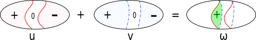
Figure 1. Illustration example to the double obstacle problem: exact coincidence sets $\Omega^{u}_{+},\Omega^{u}_{0},\Omega^{u}_{-}$ with the exact free boundary indicated by red full curves (left), approximate coincidence sets $\Omega^{v}_{+},\Omega^{v}_{0},\Omega^{v}_{-}$ with the approximate free boundary indicated by blue dash-dot curves (middle). Exact and approximate sets do not coincide and it results in an nonempty intersection set $\omega_{+}:=\Omega^{v}_{+}\cap\Omega^{u}_{0}$ filled by the green area (right), where the primal nonlinear measure $\mu_{\omega}(v)$ contributes to the error. Note that sets $\omega_{-}$ and $\omega_{\pm}$ are empty in this simple example.

For the second case, we have

(72) $$\mu^{*}_{\omega}(y^{*}):=D_{\widehat{F}}(u_{0},-\Lambda^{*}y^{*})=\int\limits_{\Omega^{u}_{+}}\left(\alpha_{+}-({\rm div}y^{*}+f)\right)u\,dx+\int\limits_{\Omega^{u}_{-}}\left(-\alpha_{-}-({\rm div}y^{*}+f)\right)u\,dx.$$

Again we may view the right hand side as a certain measure, which is zero if the sets

$$\Omega^{y^{*}}_{-}:=\left\{{\rm div}y^{*}+f+\alpha_{-}=0\right\}\qquad{\rm and}\qquad\Omega^{y^{*}}_{+}:=\left\{{\rm div}y^{*}+f-\alpha_{+}=0\right\}$$

coincide with the sets $\Omega^{u}_{-}$ and $\Omega^{u}_{+}$, respectively.

Now (4), (5), and (6) imply the following result.

Theorem 3.

Let $v\in V_{0}+u_{D}$ and $y^{*}\in Y^{*}_{{\rm div},[\alpha_{-},\alpha_{+}]}$ be approximations of $u$ and $y^{*}$, respectively. Then

(73) $${\mathds{M}}(u,v):=\frac{1}{2}||\nabla(u-v)||_{A}^{2}+\mu_{\omega}(v)=J(v)-J(u),$$

(74) $${\mathds{M}}(p^{*},y^{*}):=\frac{1}{2}||p^{*}-y^{*}||_{A^{-1}}^{2}+\mu_{\omega}^{*}(y^{*})=\widehat{I}^{*}(p^{*})-\widehat{I}^{*}(y^{*}),$$

(75) $${\mathds{M}}(\{u,p^{*}\},\{v,y^{*}\})=\frac{1}{2}\|A\nabla v-y^{*}\|^{2}_{A^{-1}}+\Upsilon(v,y^{*}),$$

where

(76) $$\Upsilon(v,y^{*}):=\int\limits_{\Omega}(\alpha_{+}(v)_{+}+\alpha_{-}(v)_{-}-(f+{\rm div}y^{*})v)\,dx$$

is a nonnegative functional, which vanishes if $y^{*}=p^{*}$ and $v=u$.

Proof.

We apply (5) and (6). Notice that $\widehat{J}(v_{0})=G(\nabla v_{0})+F(v_{0})=J(v)$. Next,

$$D_{\widehat{F}}(v_{0},-\Lambda^{*}p^{*})+D_{\widehat{G}}(\Lambda v_{0},p^{*})=\mu_{\omega}(v)+\frac{1}{2}\|A\nabla(u-v)\|^{2}_{A}.$$

It is easy to see that for any $v=v_{0}+u_{D}\in V_{0}+u_{D}$, the functional

$$J(v):=\frac{1}{2}\int\limits_{\Omega}A\nabla v\cdot\nabla v\,dx-\int\limits_{\Omega}(fv-\alpha_{+}(v)_{+}-\alpha_{(}v)_{-})dx$$

coincides with $\widehat{J}(v_{0})$ and $\widehat{J}(u_{0})$ coincides with $J(u)$. Since

$$D_{\widehat{F}}(v_{0},-\Lambda^{*}p^{*})+D_{\widehat{G}}(\Lambda v_{0},p^{*})=\widehat{J}(v_{0})-\widehat{J}(u_{0})=J(v)-J(u),$$

we arrive at (73).

Since $u_{0}=u-u_{D}$ (where $u$ satisfies the relation $A\nabla u=p^{*}$), we use (56) and (72) and obtain

$$D_{\widehat{F}}(u_{0},-\Lambda^{*}y^{*})+D_{\widehat{G}}(\Lambda u_{0},y^{*})=\mu^{*}_{\omega}(y^{*})+\frac{1}{2}||p^{*}-y^{*}||_{A^{-1}}^{2}.$$

Now (6) yields (74), where

(77) $$\widehat{I}^{*}(y^{*})=-\widehat{G}^{*}(y^{*})-\widehat{F}^{*}(-\Lambda^{*}y^{*})=-\frac{1}{2}\|y^{*}\|^{2}_{A^{-1}}+\int\limits_{\Omega}(y^{*}\cdot\nabla u_{D}+{\rm div}y^{*}u_{D})\,dx$$

(78) $$=-\frac{1}{2}\|y^{*}\|^{2}_{A^{-1}}+\int\limits_{\partial\Omega}(y^{*}\cdot n)u_{D}\,dx.$$

Finally, summation of (73) and (74) yields

(79) $${\mathds{M}}(\{u,p^{*}\},\{v,y^{*}\})=\widehat{J}(v_{0})-\widehat{I}^{*}(y^{*})=J(v)-\widehat{I}^{*}(y^{*})=\frac{1}{2}\|A\nabla v-y^{*}\|^{2}_{A^{-1}}+\Upsilon(v,y^{*}),$$

where

$$\Upsilon(v,y^{*})=\int\limits_{\Omega}(\alpha_{+}(v)_{+}+\alpha_{-}(v)_{-}-fv+y^{*}\cdot\nabla(v-u_{D})-{\rm div}y^{*}u_{D})\,dx=\int\limits_{\Omega}(\alpha_{+}(v)_{+}+\alpha_{-}(v)_{-}-(f+{\rm div}y^{*})v)\,dx.$$

∎

Corollary 2.

From (75) it follows that

(80) $$\frac{1}{2}||\nabla(u-v)||_{A}^{2}+\frac{1}{2}||p^{*}-y^{*}||_{A^{-1}}^{2}\,\leq\,\frac{1}{2}\|A\nabla v-y^{*}\|^{2}_{A^{-1}}+\Upsilon(v,y^{*}).$$

This inequality has a practical value because it provides a directly computable upper bound of the error.

Remark 5.

It is not difficult to show that $\Upsilon(v,y^{*})=0$ if and only if the set $\Omega^{y^{*}}_{<>}:=\Omega\setminus\left\{\Omega^{y^{*}}_{-}\cup\Omega^{y^{*}}_{+}\right\}$ (in this set $-\alpha_{-}<{\rm div}y^{*}+f<\alpha_{+}$) is a subset of $\Omega^{v}_{0}$, $v$ does not have positive values in $\Omega^{y^{*}}_{-}$ and negative values in $\Omega^{y^{*}}_{+}$. To prove this we represent $\Upsilon(v,y^{*})$ in the form

$$\Upsilon(v,y^{*})=\int\limits_{\Omega^{y^{*}}_{-}}(\alpha_{+}(v)_{+}+\alpha_{-}((v)_{-}+v)\,dx+\int\limits_{\Omega^{y^{*}}_{<>}}(\alpha_{+}(v)_{+}+\alpha_{-}(v)_{-}-(f+{\rm div}y^{*})v)\,dx\\ +\int\limits_{\Omega^{y^{*}}_{+}}(\alpha_{+}((v)_{+}-v)+\alpha_{-}(v)_{-})\,dx\\ =\int\limits_{\Omega^{y^{*}}_{-}}(\alpha_{+}+\alpha_{-})(v)_{+}\,dx+\int\limits_{\Omega^{y^{*}}_{<>}}(\alpha_{+}\chi_{\{v>0\}}-\alpha_{-}\chi_{\{v>0\}}-f-{\rm div}y^{*})v\,dx\\ +\int\limits_{\Omega^{y^{*}}_{+}}(\alpha_{+}+\alpha_{-})(v)_{-}\,dx=\Upsilon_{1}(v,y^{*})+\Upsilon_{2}(v,y^{*})+\Upsilon_{3}(v,y^{*}),$$

where the terms are defined by the relations

$$\Upsilon_{1}(v,y^{*})=\int\limits_{\{\Omega^{y^{*}}_{-}\cap\Omega^{v}_{+}\}\cup\{\Omega^{y^{*}}_{+}\cap\Omega^{v}_{-}\}}(\alpha_{+}+\alpha_{-})|v|\,dx,$$

$$\Upsilon_{2}(v,y^{*})=\int\limits_{\Omega^{y^{*}}_{<>}\cap\Omega^{v}_{+}}W_{+}(y^{*})|v|\,dx,\qquad\Upsilon_{3}(v,y^{*})=\int\limits_{\Omega^{y^{*}}_{<>}\cap\Omega^{v}_{-}}W_{-}(y^{*})|v|\,dx,$$

with the weights $W_{+}(y^{*})=(\alpha_{+}-f-{\rm div}y^{*})$ and $W_{-}(y^{*})=\alpha_{-}+f+{\rm div}y^{*}$. The term $\Upsilon_{1}(v,y^{*})$ vanishes if $v\leq 0$ in $\Omega^{y^{*}}_{-}$ and $v\geq 0$ in $\Omega^{y^{*}}_{+}$. In the set $\Omega^{y^{*}}_{<>}$ the weights $W_{+}(y^{*})$ and $W_{-}(y^{*})$ are positive. Therefore, $\Upsilon_{2}(v,y^{*})=\Upsilon_{3}(v,y^{*})=0$ implies $v=0$ almost everywhere in $\Omega^{y^{*}}_{<>}$, i.e., $\Omega^{y^{*}}_{<>}\subset\Omega^{v}_{0}$. If all the above conditions are satisfied, then $\Upsilon(v,y^{*})=0$ and we arrive at the identity

(81) $${\mathds{M}}(\{u,p^{*}\},\{v,y^{*}\})=\frac{1}{2}\|A\nabla v-y^{*}\|^{2}_{A^{-1}}.$$

It is clear that $\Upsilon(v,y^{*})=0$ if the set $\Omega^{v}_{-}$ coincides (up to a set of zero measure) with the set $\Omega^{y^{*}}_{-}$ and $\Omega^{v}_{+}$ coincides $\Omega^{y^{*}}_{+}$.

Remark 6.

Computable upper bound of the primal error measure ${\mathds{M}}(u,v)$ was first derived in [24]. It has the form

(82) $${\mathds{M}}(u,v)\,\leq\,{\mathds{M}}^{+}(v;\beta,\lambda_{+},\lambda_{-},y^{*})\\ :=\frac{1}{2}(1+\beta)||A\nabla v-y^{*}||_{\Omega,A^{-1}}^{2}+\frac{1}{2}(1+\frac{1}{\beta})C_{\Omega}^{2}||{\rm div}y^{*}+f-\alpha_{+}\lambda_{+}+\alpha_{-}\lambda_{-}||_{\Omega}^{2}\\ +\int\limits_{\Omega}\Big{(}\alpha_{+}\big{(}v_{+}-\lambda_{+}v\big{)}+\alpha_{-}\big{(}v_{-}+\lambda_{-}v\big{)}\Big{)}\,dx.$$

The majorant ${\mathds{M}}^{+}$ contains contains free variables: $\beta>0$, $y^{*}\in Y^{*}_{{\rm div}}(\Omega)$, and two nonnegative functions (Lagrange multipliers) $\lambda_{+},\lambda_{-}\in L^{2}(\Omega)$ satisfying $\lambda_{+}(x),\lambda_{-}(x)\in[0,1]$ almost for all $x\in\Omega$. The constant $C_{\Omega}>0$ is given by (39). In practical computations [5] it is convenient to simplify ${\mathds{M}}^{+}(v;\beta,\lambda_{+},\lambda_{-},y^{*})$ to

(83) $$\qquad{\mathds{M}}_{1}^{+}(v;\beta,\lambda,y^{*}):=\frac{1}{2}(1+\beta)||A\nabla v-y^{*}||_{\Omega,A^{-1}}^{2}+\frac{1}{2}(1+\frac{1}{\beta})C_{\Omega}^{2}||{\rm div}y^{*}+f-\lambda||_{\Omega}^{2}+\int\limits_{\Omega}(\alpha_{+}v_{+}+\alpha_{-}v_{-}-\lambda v)\,dx,$$

where only one multiplier $\lambda\in L^{2}(\Omega)$ satisfying $\lambda\in[-\alpha_{-},\alpha_{+}]$ almost for all $x\in\Omega$ is required.

4. Numerical verifications of the error identities

4.1. The classical obstacle problem

We consider an example from [13] with known exact solution. Here,

$$\Omega=(0,1),\qquad f=const<0,\qquad A=1,\qquad\phi=const<0$$

and $u$ satisfies the homogeneous Dirichlet boundary conditions $u(0)=0,u(1)=0.$ The exact solution $u$ is in the form

(84) $$u(x)=u_{f,\phi}(x)=\left\{\begin{array}[]{lrl}\vskip 6.0pt plus 2.0pt minus 2.0pt-\frac{f}{2}x^{2}-\sqrt{2f\phi}\,x&\quad\textrm{if}&x\in[0,\frac{1}{2}-r]\\ \vskip 6.0pt plus 2.0pt minus 2.0pt\phi&\quad\textrm{if}&x\in(\frac{1}{2}-r,\frac{1}{2}+r)\\ \vskip 6.0pt plus 2.0pt minus 2.0pt-\frac{f}{2}(x-1)^{2}+\sqrt{2f\phi}\,(x-1)&\quad\textrm{if}&x\in[\frac{1}{2}+r,1]\end{array}\right.$$

where $r=r_{f,\phi}:=\frac{1}{2}-\sqrt{\frac{2\phi}{f}}\in(0,\frac{1}{2})$. The parameter $r$ determines the radius of the exact lower coincidence set

$$\Omega^{u}_{-}=(\frac{1}{2}-r,\frac{1}{2}+r).$$

It is easy to show that the exact energy reads

$$J(u)=f\phi(\frac{4}{3}\sqrt{\frac{2\phi}{f}}-1).$$

An approximation $v_{\epsilon_{1}}$ is considered in the form of $u$ corresponding to the same value of $\phi$ and a perturbed value $f$,

$$v_{\epsilon_{1}}(x):=u_{f_{\epsilon_{1}},\phi}(x),\qquad f_{\epsilon_{1}}:=\frac{2\phi}{(\frac{1}{2}-r+\epsilon_{1})^{2}}$$

for some small perturbation $\epsilon_{1}$. This choice ensures

$$\Omega^{v_{\epsilon_{1}}}_{-}=(\frac{1}{2}-r+\epsilon_{1},\frac{1}{2}+r-\epsilon_{1})\qquad\mbox{for }\epsilon_{1}\in(r-\frac{1}{2},r)$$

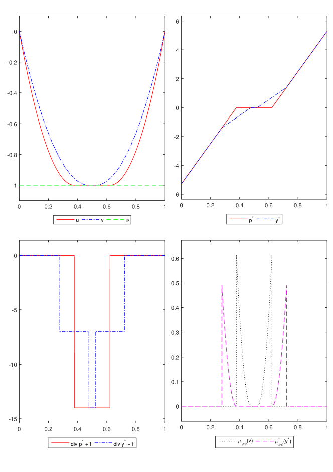
Figure 2. Example of the classical obstacle problem with $\phi=-1$ and $f=-14$ and approximations $v_{\epsilon_{1}}$ and $y^{*}_{\epsilon_{2}}$ generated by perturbations $\epsilon_{1}=\epsilon_{2}=0.1.$ The exact solution $u$ and its approximation $v_{\epsilon_{1}}$ are displayed in the top left picture, the exact flux $p^{*}=u^{\prime}$ and its approximation $y^{*}_{\epsilon_{2}}$ in the top right picture. Both nonpositive functions ${\rm div}\,p^{*}+f$ and ${\rm div}\,y^{*}_{\epsilon_{2}}+f$ are displayed in the bottom left picture. Since $\Omega^{v}_{-}\subset\Omega^{u}_{-}$ and $\subset\Omega^{u}_{-}\subset\Omega^{y^{*}}_{-}$ , there are positive contributions of $\mu_{\phi\psi}(v_{\epsilon_{1}})$ and $\mu_{\phi\psi}^{*}(y^{*}_{\epsilon_{2}})$ shown in the bottom right picture.

and in particular, $\Omega^{v_{\epsilon_{1}}}_{-}\subset\Omega^{u}_{-}$ for $\epsilon_{1}\in(0,r)$. An example of $u$ and $v_{\epsilon_{1}}$ is depicted in the top left picture of Figure 2. An approximation $y^{*}_{\epsilon_{2}}$ is taken as

$$y^{*}_{\epsilon_{2}}(x)=I(p^{*})(x),\qquad x\in\Omega,$$

where $I$ denotes a piecewise linear nodal and continuous interpolation operator at nodes

$$\{0,\frac{1}{2}-r-\epsilon_{2},\frac{1}{2}-r+\epsilon_{2},\frac{1}{2}+r-\epsilon_{2},\frac{1}{2}+r+\epsilon_{2},1\}$$

for some small positive perturbation $\epsilon_{2}$. The approximation $y^{*}_{\epsilon_{2}}$ differs from the exact flux $p^{*}$ only locally in $(\frac{1}{2}-r-\epsilon_{2},\frac{1}{2}-r+\epsilon_{2})\cup(\frac{1}{2}+r-\epsilon_{2},\frac{1}{2}+r+\epsilon_{2})$ and

$$\Omega^{u}_{-}\subset\Omega^{y^{*}_{\epsilon_{2}}}_{-}=(\frac{1}{2}-r-\epsilon_{2},\frac{1}{2}+r+\epsilon_{2})\quad\mbox{for }\epsilon_{2}\in(0,r).$$

An example of $p^{*}$ and $y^{*}_{\epsilon_{2}}$ is shown in the top right picture of Figure 2 and corresponding equilibrium terms ${\rm div}p^{*}+f$ and ${\rm div}y^{*}_{\epsilon_{2}}+f$ in the bottom left picture.

For numerical verifications, we choose parameters

$$\phi=-1,\quad f=-14$$

resulting in $r\approx 0.1220$, $J(u)\approx-6.9446$ and approximations $v_{\epsilon_{1}},y^{*}_{\epsilon_{2}}$ corresponding to

$$\epsilon_{1},\epsilon_{2}\in\{1/10,1/20,1/40,1/80,1/160\}.$$

We first verify the primal error identity

$$\frac{1}{2}\|\nabla(u-v_{\epsilon_{1}})\|^{2}+\mu_{\phi\psi}(v_{\epsilon_{1}})={\mathds{M}}(u,v_{\epsilon_{1}})=J(v_{\epsilon_{1}})-J(u)$$

for all approximations $v_{\epsilon_{1}}$. Table 3 confirms that the primal error identity holds and both quadratic (gradient containing) and nonlinear parts of the primal error converge. For smaller values of $\epsilon_{1}$ the quadratic part dominates over the nonlinear part. This is due to the fact that the quadratic part of error is globally distributed over $\Omega$ and the nonlinear part $\mu_{\phi\psi}(v_{\epsilon_{1}})$ has a support in

$$\Omega^{u}_{-}\setminus\Omega^{v_{\epsilon_{1}}}_{-}\approx(0.3779,0.3779+\epsilon_{1})\,\cup\,(0.6220-\epsilon_{1},0.6220).$$

Table 3 verifies the dual error identity

$$\frac{1}{2}\|p^{*}-y^{*}_{\epsilon_{2}}\|^{2}+\mu_{\phi\psi}^{*}(y^{*}_{\epsilon_{2}})={\mathds{M}}(p^{*},y^{*}_{\epsilon_{2}})=I^{*}(p^{*})-I^{*}(y^{*}_{\epsilon_{2}})$$

for all approximations $y^{*}_{\epsilon_{2}}$. Again, both quadratic and nonlinear parts converge. None of error parts dominates, since $y^{*}_{\epsilon_{2}}$ and $p^{*}_{\epsilon_{2}}$ differ only locally. The nonlinear part $\mu_{\phi\psi}^{*}(y^{*}_{\epsilon_{2}})$ has a support in

$$\Omega^{y^{*}_{\epsilon_{2}}}_{-}\setminus\Omega^{u}_{-}\approx(0.3779-\epsilon_{2},0.3779)\,\cup\,(0.6220,0.6220+\epsilon_{2}).$$

An example of primal and dual nonlinear error functions is depicted in the bottom left picture of of Figure 2.

Table 3 verifies the majorant identity

$${\mathds{M}}(\{u,p^{*}\},\{v_{\epsilon_{1}},y^{*}_{\epsilon_{2}}\})=\frac{1}{2}||A\nabla v_{\epsilon_{1}}-y^{*}_{\epsilon_{2}}||^{2}+\Upsilon(v_{\epsilon_{1}},y^{*}_{\epsilon_{2}}),$$

where the computable nonlinear majorant part $\Upsilon$ is given by (33). The majorant identity is valid for all considered approximations.

Remark 7.

Since the upper obstacle $\psi$ is not considered in this example,

$${\rm div}y^{*}+f\leq 0\qquad\mbox{in }\Omega$$

has to be satisfied. This condition is fulfilled for $y^{*}_{\epsilon_{2}}$ constructed above.

4.2. The double obstacle problem

We consider an example with known exact solution. Here,

$$\Omega=(-1,1),\qquad f=0,\qquad A=1,\qquad\alpha_{+},\alpha_{-}>2$$

and $u$ satisfies Dirichlet boundary conditions $u(-1)=-1,u(1)=1.$ This example generalizes example of [4], in which $\alpha_{+}=\alpha_{-}=8$. It is possible to show the exact solution is given by a formula

$$u(x)=u_{\alpha_{-},\alpha_{+}}(x)=\left\{\begin{array}[]{ll}-(\frac{\alpha_{-}}{2})\,x^{2}+(\sqrt{2\alpha_{-}}-\alpha_{-})\,x+\sqrt{2\alpha_{-}}-\frac{\alpha_{-}}{2}-1,&x\in\left<-1,r_{-}\right>,\\ 0,&x\in(r_{-},r_{+}),\\ (\frac{\alpha_{+}}{2})\,x^{2}+(\sqrt{2\alpha_{+}}-\alpha_{+})\,x-\sqrt{2\alpha_{+}}+\frac{\alpha_{+}}{2}+1,&x\in\left<r_{+},1\right>,\end{array}\right.$$

where $r_{-}:=\sqrt{\frac{2}{\alpha_{-}}}-1\in(-1,0)$ and $r_{+}:=1-\sqrt{\frac{2}{\alpha_{+}}}\in(0,1)$ determine exact coincidence sets

$$\Omega^{u}_{-}=(-1,r_{-}),\qquad\Omega^{u}_{0}=\left<r_{-},r_{+}\right>,\qquad\Omega^{u}_{+}=(r_{+},1).$$

The exact energy then reads

$$J(u)=\frac{2\sqrt{2}}{3}(\sqrt{\alpha_{+}}+\sqrt{\alpha_{-}}).$$

An approximation $v_{\epsilon_{1}}$ is considered in the form of $u$ corresponding to perturbed values $\alpha_{+}$, $\alpha_{-}$,

$$v_{\epsilon_{1}}(x):=u_{\alpha_{-_{\epsilon_{1}}},\alpha_{+_{\epsilon_{1}}}},\qquad\alpha_{\pm_{\epsilon_{1}}}:=\frac{2}{(1\mp r_{\pm}+\epsilon_{1})^{2}}$$

for some small perturbation $\epsilon_{1}$. This choice ensures

$$\Omega^{v_{\epsilon_{1}}}_{0}=(r_{-}+\epsilon_{1},r_{+}-\epsilon_{1})\qquad\mbox{for }\epsilon_{1}\in(-1+r_{+},r_{+})\cap(-1-r_{-},-r_{-})$$

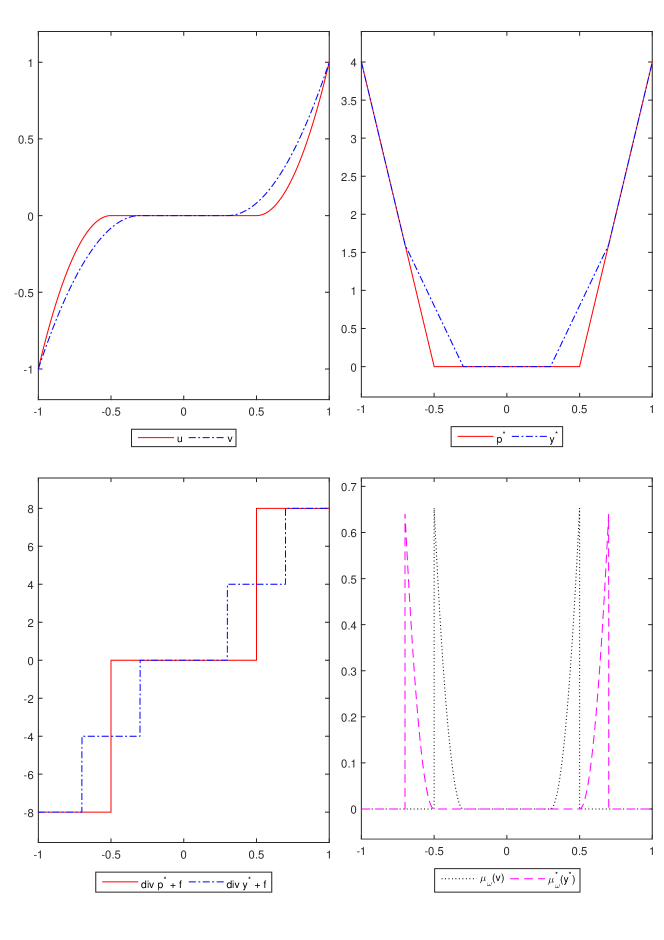
Figure 3. Example of the double obstacle problem with $\alpha_{+}=\alpha_{-}=8$ and approximations $v_{\epsilon_{1}}$ and $y^{*}_{\epsilon_{2}}$ generated by perturbations $\epsilon_{1}=\epsilon_{2}=0.2.$ The exact solution $u$ and its approximation $v_{\epsilon_{1}}$ are displayed in the top left picture, the exact flux $p^{*}=u^{\prime}$ and its approximation $y^{*}_{\epsilon_{2}}$ in the top right picture. Both nonpositive functions ${\rm div}\,p^{*}+f$ and ${\rm div}\,y^{*}_{\epsilon_{2}}+f$ are displayed in the bottom left picture. Since $\Omega^{v}_{-}\subset\Omega^{u}_{-}$ and $\subset\Omega^{u}_{-}\subset\Omega^{y^{*}}_{-}$ , there are positive contributions of $\mu_{\omega}(v_{\epsilon_{1}})$ and $\mu_{\omega}^{*}(y^{*}_{\epsilon_{2}})$ shown in the bottom right picture.)

and in particular, $\Omega^{v_{\epsilon_{1}}}_{0}\subset\Omega^{u}_{0}$ for $\epsilon_{1}\in(0,\min\{r_{+},-r_{-}\})$. An example of $u$ and $v_{\epsilon_{1}}$ is depicted in the top left picture of Figure 3. An approximation $y^{*}_{\epsilon_{2}}$ is taken as

$$y^{*}_{\epsilon_{2}}(x)=I(p^{*})(x),\qquad x\in\Omega,$$

where $I$ denotes a piecewise linear nodal and continuous interpolation operator at nodes

$$\{-1,r_{-}-\epsilon_{2},r_{-}+\epsilon_{2},r_{+}-\epsilon_{2},r_{+}+\epsilon_{2},1\}$$

for some small positive perturbation $\epsilon_{2}$. The approximation $y^{*}_{\epsilon_{2}}$ differs from the exact flux $p^{*}$ only locally in $(r_{-}-\epsilon_{2},r_{-}+\epsilon_{2})\cup(r_{+}-\epsilon_{2},r_{+}+\epsilon_{2})$ and

$$\Omega^{u}_{-}\subset\Omega^{y^{*}_{\epsilon_{2}}}_{-}=(r_{-}-\epsilon_{2},r_{+}+\epsilon_{2})\quad\mbox{for }\epsilon_{2}\in(0,\min\{-r_{-},r_{+}\}).$$

An example of $p^{*}$ and $y^{*}_{\epsilon_{2}}$ is shown in the top right picture of Figure 3 and corresponding equilibrium terms in the bottom left picture.

For numerical verifications, we choose parameters (identical to example of [4])

$$\alpha_{-}=\alpha_{+}=8$$

resulting in

$$u(x)=\left\{\begin{array}[]{ll}-4x^{2}-4x-1,&x\in\left<-1,-0.5\right>,\\ 0,&x\in(-0.5,0.5),\\ 4x^{2}-4x+1,&x\in\left<0.5,1\right>\end{array}\right.$$

and $J(u)=5\frac{1}{3}$ and approximations $v_{\epsilon_{1}},y^{*}_{\epsilon_{2}}$ corresponding to

$$\epsilon_{1},\epsilon_{2}\in\{1/5,1/10,1/20,1/40,1/80\}.$$

We again verify the primal error identity

$$\frac{1}{2}\|\nabla(u-v_{\epsilon_{1}})\|^{2}+\mu_{\omega}(v_{\epsilon_{1}})={\mathds{M}}(u,v_{\epsilon_{1}})=J(v_{\epsilon_{1}})-J(u)$$

for all approximations $v_{\epsilon_{1}}$. Table 6 confirms that the primal error identity holds and both quadratic (gradient containing) and nonlinear parts of the primal error converge. For smaller values of $\epsilon_{1}$ the quadratic part dominates over the nonlinear part. This is due to the fact that the quadratic part of error is globally distributed over $\Omega$ and the nonlinear part $\mu_{\phi\psi}(v_{\epsilon_{1}})$ has a support in

$$\Omega^{u}_{-}\setminus\Omega^{v_{\epsilon_{1}}}_{-}\approx(-0.5,-0.5+\epsilon_{1})\,\cup\,(0.5-\epsilon_{1},0.5).$$

Table 6 verifies the dual error identity

$$\frac{1}{2}\|p^{*}-y^{*}_{\epsilon_{2}}\|^{2}+\mu_{\omega}^{*}(y^{*}_{\epsilon_{2}})={\mathds{M}}(p^{*},y^{*}_{\epsilon_{2}})=I^{*}(p^{*})-I^{*}(y^{*}_{\epsilon_{2}})$$

for all approximations $y^{*}_{\epsilon_{2}}$. Again, both quadratic and nonlinear parts converge. None of error parts dominates, since $y^{*}_{\epsilon_{2}}$ and $p^{*}_{\epsilon_{2}}$ differ only locally. The nonlinear part $\mu_{\phi\psi}^{*}(y^{*}_{\epsilon_{2}})$ has a support in

$$\Omega^{y^{*}_{\epsilon_{2}}}_{-}\setminus\Omega^{u}_{-}\approx(0.5-\epsilon_{2},0.5)\,\cup\,(0.5,0.5+\epsilon_{2}).$$

An example of primal and dual nonlinear error functions is depicted in the bottom left picture of of Figure 3.

Table 6 verifies the majorant identity

$${\mathds{M}}(\{u,p^{*}\},\{v_{\epsilon_{1}},y^{*}_{\epsilon_{2}}\})=\frac{1}{2}||A\nabla v_{\epsilon_{1}}-y^{*}_{\epsilon_{2}}||^{2}+\Upsilon(v_{\epsilon_{1}},y^{*}_{\epsilon_{2}}),$$

where the computable nonlinear majorant part $\Upsilon$ is given by (76). The majorant identity is valid for all considered approximations.

$\epsilon_{1}$	$\frac{1}{2}\|\nabla(u-v_{\epsilon_{1}})\|^{2}$	$\mu_{\phi\psi}(v_{\epsilon_{1}})$	${\mathds{M}}(u,v_{\epsilon_{1}})$	$J(v_{\epsilon_{1}})-J(u)$	$\mu_{\phi\psi}(v_{\epsilon_{1}})$ [%]
0.1000	1.54e-01	4.09e-02	1.95e-01	1.95e-01	20.92
0.0500	4.82e-02	6.37e-03	5.45e-02	5.45e-02	11.68
0.0250	1.36e-02	8.98e-04	1.45e-02	1.45e-02	6.20
0.0125	3.62e-03	1.20e-04	3.73e-03	3.73e-03	3.20
0.0063	9.33e-04	1.54e-05	9.49e-04	9.49e-04	1.63

Table 1. Terms in the primal error identity computed for various approximation $v_{\epsilon_{1}}$ in case of the classical obstacle in 1D. The rightmost column shows the contribution of $\mu_{\phi\psi}(v_{\epsilon_{1}})$ to the majorant value ${\mathds{M}}(u,v_{\epsilon_{1}})$.

$\epsilon_{2}$	$\frac{1}{2}\|p^{*}-y^{*}_{\epsilon_{2}}\|^{2}$	$\mu_{\phi\psi}^{*}(y^{*}_{\epsilon_{2}})$	${\mathds{M}}(p^{*},y^{*}_{\epsilon_{2}})$	$I^{*}(p^{*})-I^{*}(y^{*}_{\epsilon_{2}})$	$\mu_{\phi\psi}^{*}(y^{*}_{\epsilon_{2}})$ [%]
0.0500	4.08e-03	4.08e-03	8.17e-03	8.17e-03	50.00
0.0250	5.10e-04	5.10e-04	1.02e-03	1.02e-03	50.00
0.0125	6.38e-05	6.38e-05	1.28e-04	1.28e-04	50.00
0.0063	7.98e-06	7.98e-06	1.60e-05	1.60e-05	50.00
0.0031	9.97e-07	9.97e-07	1.99e-06	1.99e-06	50.00

Table 2. Terms in the dual error identity computed for various approximation $y^{*}_{\epsilon_{2}}$ in case of the classical obstacle in 1D. The rightmost column shows the contribution of $\mu_{\phi\psi}^{*}(y^{*}_{\epsilon_{2}})$ to the majorant value ${\mathds{M}}(p^{*},y^{*}_{\epsilon_{2}})$.

$\epsilon_{1}$	$\epsilon_{2}$	$\frac{1}{2}||\nabla v_{\epsilon_{1}}-y^{*}_{\epsilon_{2}}||^{2}$	$\Upsilon(v_{\epsilon_{1}},y^{*}_{\epsilon_{2}})$	sum	${\mathds{M}}(\{u,p^{*}\},\{v_{\epsilon_{1}},y^{*}_{\epsilon_{2}}\})$
0.1000	0.1000	9.72e-02	1.63e-01	2.61e-01	2.61e-01
0.1000	0.0500	1.32e-01	7.15e-02	2.03e-01	2.03e-01
0.0500	0.0500	3.72e-02	2.55e-02	6.27e-02	6.27e-02
0.0500	0.0250	4.44e-02	1.11e-02	5.55e-02	5.55e-02
0.0250	0.0250	1.19e-02	3.59e-03	1.55e-02	1.55e-02
0.0250	0.0125	1.30e-02	1.57e-03	1.46e-02	1.46e-02
0.0125	0.0125	3.38e-03	4.78e-04	3.86e-03	3.86e-03
0.0125	0.0063	3.54e-03	2.09e-04	3.75e-03	3.75e-03
0.0063	0.0063	9.03e-04	6.17e-05	9.65e-04	9.65e-04
0.0063	0.0031	9.24e-04	2.70e-05	9.51e-04	9.51e-04

Table 3. Terms in the majorant error identity computed for various approximation $v_{\epsilon_{1}}$ and $y^{*}_{\epsilon_{2}}$ in case of the classical obstacle in 1D. The computable majorant $\frac{1}{2}||\nabla v_{\epsilon_{1}}-y^{*}_{\epsilon_{2}}||^{2}+\Upsilon(v_{\epsilon_{1}},y^{*}_{\epsilon_{2}})$ is identical to ${\mathds{M}}(\{u,p^{*}\},\{v_{\epsilon_{1}},y^{*}_{\epsilon_{2}}\})$, which can only be computed with the knowledge of the exact solution $u$ and the exact flux $p^{*}$.

$\epsilon_{1}$	$\frac{1}{2}\|\nabla(u-v_{\epsilon_{1}})\|^{2}$	$\mu_{\omega}(v_{\epsilon_{1}})$	${\mathds{M}}(u,v_{\epsilon_{1}})$	$J(v_{\epsilon_{1}})-J(u)$	$\mu_{\omega}(v_{\epsilon_{1}})$ [%]
0.2000	2.18e-01	8.71e-02	3.05e-01	3.05e-01	28.57
0.1000	7.41e-02	1.48e-02	8.89e-02	8.89e-02	16.67
0.0500	2.20e-02	2.20e-03	2.42e-02	2.42e-02	9.09
0.0250	6.05e-03	3.02e-04	6.35e-03	6.35e-03	4.76
0.0125	1.59e-03	3.97e-05	1.63e-03	1.63e-03	2.44

Table 4. Terms in the primal error identity computed for various approximation $v_{\epsilon_{1}}$ in case of the double obstacle in 1D. The rightmost column shows the contribution of $\mu_{\phi\psi}(v_{\epsilon_{1}})$ to the majorant value ${\mathds{M}}(u,v_{\epsilon_{1}})$.

$\epsilon_{2}$	$\frac{1}{2}\|p^{*}-y^{*}_{\epsilon_{2}}\|^{2}$	$\mu_{\omega}^{*}(y^{*}_{\epsilon_{2}})$	${\mathds{M}}(p^{*},y^{*}_{\epsilon_{2}})$	$I^{*}(p^{*})-I^{*}(y^{*}_{\epsilon_{2}})$	$\mu_{\omega}^{*}(y^{*}_{\epsilon_{2}})$ [%]
0.2000	8.53e-02	8.53e-02	1.71e-01	1.71e-01	50.00
0.1000	1.07e-02	1.07e-02	2.13e-02	2.13e-02	50.00
0.0500	1.33e-03	1.33e-03	2.67e-03	2.67e-03	50.00
0.0250	1.67e-04	1.67e-04	3.33e-04	3.33e-04	50.00
0.0125	2.08e-05	2.08e-05	4.17e-05	4.17e-05	50.00

Table 5. Terms in the dual error identity computed for various approximation $y^{*}_{\epsilon_{2}}$ in case of the double obstacle in 1D. The rightmost column shows the contribution of $\mu_{\phi\psi}^{*}(y^{*}_{\epsilon_{2}})$ to the majorant value ${\mathds{M}}(p^{*},y^{*}_{\epsilon_{2}})$.

$\epsilon_{1}$	$\epsilon_{2}$	$\frac{1}{2}||\nabla v_{\epsilon_{1}}-y^{*}_{\epsilon_{2}}||^{2}$	$\Upsilon(v_{\epsilon_{1}},y^{*}_{\epsilon_{2}})$	sum	${\mathds{M}}(\{u,p^{*}\},\{v_{\epsilon_{1}},y^{*}_{\epsilon_{2}}\})$
0.2000	0.2000	1.27e-01	3.48e-01	4.75e-01	4.75e-01
0.1000	0.2000	5.96e-02	2.00e-01	2.60e-01	2.60e-01
0.1000	0.1000	5.10e-02	5.93e-02	1.10e-01	1.10e-01
0.0500	0.1000	1.58e-02	2.98e-02	4.56e-02	4.56e-02
0.0500	0.0500	1.81e-02	8.82e-03	2.69e-02	2.69e-02
0.0250	0.0500	4.93e-03	4.08e-03	9.02e-03	9.02e-03
0.0250	0.0250	5.47e-03	1.21e-03	6.68e-03	6.68e-03
0.0125	0.0250	1.42e-03	5.35e-04	1.96e-03	1.96e-03
0.0125	0.0125	1.51e-03	1.59e-04	1.67e-03	1.67e-03
0.0063	0.0125	3.85e-04	6.86e-05	4.53e-04	4.53e-04

Table 6. Terms in the majorant error identity computed for various approximation $v_{\epsilon_{1}}$ and $y^{*}_{\epsilon_{2}}$ in case of the double obstacle in 1D. The computable majorant $\frac{1}{2}||\nabla v_{\epsilon_{1}}-y^{*}_{\epsilon_{2}}||^{2}+\Upsilon(v_{\epsilon_{1}},y^{*}_{\epsilon_{2}})$ is identical to ${\mathds{M}}(\{u,p^{*}\},\{v_{\epsilon_{1}},y^{*}_{\epsilon_{2}}\})$, which can only be computed with the knowledge of the exact solution $u$ and the exact flux $p^{*}$.

References

- [1] H. Brezis, Problémes unilatéraux, J. Math. Pures Appl. 9 (1971), 1–168.
- [2] H. Brezis and M. Sibony, Equivalence de deux inequations variationnelles et applications, Arch. Rat. Mech. Anal., 41(1971), 254–265.
- [3] F. Brezzi, W. Hager, and P.-A. Raviart, Error estimates for the finite element solution of variational inequalities. II. Mixed methods. Numer. Math. 31 (1978), no. 1, 1–16.
- [4] F. Bozorgnia, Numerical solutions of a two-phase membrane problem, Applied Numerical Mathematics 61 (2011), no. 1, 92–107.
- [5] F. Bozorgnia and J. Valdman, A FEM approximation of a two-phase obstacle problem and its a posteriori error estimate, Computers & Mathematics with Applications 73 (2017), no. 3, 419–432.
- [6] H. Buss and S. Repin, A posteriori error estimates for boundary value problems with obstacles, Proceedings of 3nd European Conference on Numerical Mathematics and Advanced Applications, Jÿvaskylä, 1999, World Scientific, 162–170, 2000.
- [7] L.A. Caffarelli, The obstacle problem revisited, J. Fourier Anal. Appl. 4 (1998), 383–402.
- [8] G. Duvaut and G.-L. Lions. Inequalities in mechanics and physics. Springer, Berlin-New York, 1976.
- [9] R. S. Falk. Error estimates for the approximation of a class of variational inequalities. Journal Mathematics of Computations, 28 (1974), no. 128, 963–971.
- [10] A. Friedman, Variational principles and free-boundary problems, Wiley, New York (1982).
- [11] R. Glowinski, Numerical Methods for Nonlinear Variational Problems, Springer Verlag, New York, New York, 1984.
- [12] R. Glowinski, J.-L. Lions, and R. Tremolieres, Numerical Analysis of Variational Inequalities, North-Holland, Amsterdam, Holland, 1981.
- [13] P. Harasim, J. Valdman. Verification of functional a posteriori error estimates for obstacle problem in 1D. Kybernetika, 49 (5), 738 – 754, 2013.
- [14] P. Harasim, J. Valdman. Verification of functional a posteriori error estimates for obstacle problem in 2D. Kybernetika, 50 (6), 978 – 1002, 2014.
- [15] T. Kärkkäinen, K. Kunisch, and P. Tarvainen. Augmented Lagrangian active set methods for obstacle problems. J. Optim. Theory Appl. 119 (2003), no. 3, 499–533.
- [16] D. Kinderlehrer and G. Stampacchia, An introduction to variational inequalities and their applications, Academic Press, New York, 1980.
- [17] P. Neittaanmäki and S. Repin, Reliable Methods for Computer Simulation. Error Control and a Posteriori Estimates, Elsevier, Amsterdam (2004).
- [18] I. Ekeland and R. Temam, Convex Analysis and Variational Problems, North-Holland, Amsterdam (1976).
- [19] S. Repin, A Posteriori Estimates for Partial Differential Equations, Walter de Gruyter, Berlin (2008).
- [20] S. Repin, A posteriori error estimates for approximate solutions to variational problems with strongly convex functionals. Journal of Mathematical Sciences. Vol. 97, No. 4, 1999.
- [21] S. Repin. A posteriori error estimation for variational problems with uniformly convex functionals, Math. Comp. 69, No. 230, 481–500 (2000).
- [22] S. Repin, Estimates of deviations from exact solutions of elliptic variational inequalities, J. Math. Sci., 115, No. 6, 2811–2819 (2003).
- [23] S. Repin, On measures of errors for nonlinear variational problems, Russ. J. Numer. Anal. Math. Model. 27, No. 6, 577–584 (2012).
- [24] S. Repin and J. Valdman, A posteriori error estimates for two-phase obstacle problem, J. Math.Sci. 20, No. 2, 324–336 (2015)
- [25] H. Shahgholian, N. N. Uraltseva, G. S.Weiss, The two-phase membrane problem regularity of the free boundaries in higher dimensions, Int. Math. Res. Not. 2007, No. 8, ID rnm026 (2007).
- [26] P. Tarvainen, Two-Level Schwarz Method for Unilateral Variational Inequalities, IMA Journal of Numerical Analysis, Vol. 19, pp. 193?212, 1999.
- [27] G. S. Weiss, The two-phase obstacle problem: pointwise regularity of the solution and an estimate of the Hausdorff dimension of the free boundary. Interfaces Free Bound. 3, No. 2, 121–128 (2001).
- [28] N. N. Uraltseva, Regularity of solutions of variational inequalities,” Usp. Mat. Nauk, 42, No. 6(258), 151–174 (1987).
- [29] N.N. Uraltseva, Two-phase obstacle problem. Problems in Math.Analysis, v 22, 2001, 240–245 (in Russian. English translation: Journal of Math Sciences, v.106, N 3, 2001, pp. 3073-3078)