Fast and slow thermal processes in harmonic scalar lattices

Abstract

An approach for analytical description of thermal processes in harmonic lattices is presented. We cover longitudinal and transverse vibrations of chains and out-of-plane vibrations of two-dimensional lattices with interactions of an arbitrary number of neighbors. Motion of each particle is governed by a single scalar equation and therefore the notion “scalar lattice” is used. Evolution of initial temperature field in an infinite lattice is investigated. An exact equation describing the evolution is derived. Continualization of this equation with respect to spatial coordinates is carried out. The resulting continuum equation is solved analytically. The solution shows that the kinetic temperature is represented as the sum of two terms, one describing short time behavior, the other large time behavior. At short times, the temperature performs high-frequency oscillations caused by redistribution of energy among kinetic and potential forms (fast process). Characteristic time of this process is of order of ten periods of atomic vibrations. At large times, changes of the temperature are caused by ballistic heat transfer (slow process). The temperature field is represented as a superposition of waves having the shape of initial temperature distribution and propagating with group velocities dependent on the wave vector. Expressions describing fast and slow processes are invariant with respect to substitution $t$ by $-t$. However examples considered in the paper demonstrate that these processes are irreversible. Numerical simulations show that presented theory describes the evolution of temperature field at short and large time scales with high accuracy.

PACS: 05.60.Cd, 44.10.+i, 63.20.-e, 63.22.-m, 66.70.-f
Keywords: ballistic heat transfer, harmonic crystal, scalar lattice, covariance, kinetic temperature.

1 Introduction

At macrolevel, heat propagation is usually diffusive and well-described by the Fourier law. The law assumes linear dependence between the heat flux and temperature gradient with proportionality coefficient refereed to as the heat conductivity. Phonon theory relates the heat conductivity coefficient with the phonon mean free path [1, 2]. It is assumed that the Fourier law is valid if the mean free path is much smaller than characteristic size of the system. At micro- and nanolevel, this condition may be violated. In particular, it is shown experimentally that the mean free path can be as large as several microns [3]. In this case, the heat transport is ballistic [3, 4, 5, 6, 7, 8, 9] and can not be described by the Fourier law. In particular, the effective heat conductivity is size-dependent [4, 5, 6] and it can not be regarded as a material constant. This phenomenon leads to a variety of practical applications of heat transport in micro- and nanosystems (see e.g. review paper [10]). On the other hand, derivation of macroscopic heat transport equations from lattice dynamics equations is a serious challenge for theoreticians [11].

One of the convenient models for investigation of heat transport in solids is a harmonic crystal. Heat transport in harmonic crystals is usually investigated in a steady-state regime. Stationary temperature distribution between two reservoirs with different temperatures is considered. For example, in a pioneering work by Reider, Lebowitz and Lieb [12], anomalies of the heat transport in one-dimensional harmonic chain with nearest neighbor interactions are demonstrated and an analytical solution of the steady heat transport problem is derived. The solution shows that thermal resistance of the chain is independent on its length. Therefore the effective heat conductivity diverges with length and the Fourier law is not applicable.

Anomalous heat transport is also observed in more complicated harmonic systems. Generalization of results obtained in paper [12] for the multidimensional case is carried out in papers [13, 14]. Harmonic chains with alternating masses are considered in paper [15]. The effect of disorder on heat transport in harmonic crystals is studied in papers [16, 17, 18, 19]. The influence of conservative bulk noises on nonequilibrium steady state is investigated in papers [20, 21, 22, 23]. Solution of the steady-state problem for an arbitrary harmonic network is obtained in paper [24]. Specific feature of the stationary heat transfer problem considered in the above mentioned papers is that the results strongly depend on the type of thermostat [25, 26, 27]. For example, in paper [27] it is shown that a specific choice of the thermostat leads to Fourier heat conduction in harmonic crystals. Note that the influence of thermostat is also observed in nonlinear systems [28].

The present paper focuses on unsteady thermal processes. Evolution of initial temperature field in an infinite lattice is considered. It allows us to investigate properties of the lattice, rather than properties of the thermostat. We consider the initial conditions typical for molecular dynamics simulations of the heat transfer [29, 30, 31, 32, 33, 34, 35, 36, 37]. Initially, particles have random velocities corresponding to the initial temperature field. Initial displacements are equal to zero. In this case, initial kinetic and potential energies are not equal. Motion of particles leads to redistribution of energy between kinetic and potential forms. After some time the energies become equal as predicted by the virial theorem [38]. However the theorem does not describe the transient process. This process is important in particular because it determines the short time behavior of the kinetic temperature. Analytical description of the transient process is reported only for several particular systems [39, 40, 41]. At large time scale, kinetic and potential energies are practically equal and changes of kinetic temperature are caused by the energy transport. Rigorous mathematical description of large time behavior of energy density for harmonic lattices in continuum limit is presented in papers [42, 43, 44, 45, 46]. Short time behavior of kinetic temperature is not considered in these works.

The main goal of the present paper is to develop an approach for analytical description of short and large time behavior of the kinetic temperature. A wide class of one- and two-dimensional lattices with interactions of an arbitrary number of neighbors and harmonic on-site potential is considered. The approach is based on analysis of velocity covariances for all pairs of particles. A deterministic equation exactly describing the evolution of temperature field is derived (section 3). Continualization of this equation with respect to spatial coordinates is carried out (section 4). The resulting continuum equation is solved analytically (section 5). The expression for the temperature field, valid at both short and large time scales, is obtained. At short times, it describes oscillations of temperature caused by equilibration of kinetic and potential energies (fast process). From a practical viewpoint, the description of the fast process is important for modeling of fempto- and attosecond laser excitation [47, 48, 49, 50]. At large time scale, the expression describes the ballistic heat transfer (slow process). Large time behavior of the solution is consistent with results obtained in papers [42, 43, 44, 45, 46]. Additionally, the present work contains detailed analysis of several physically important cases, such as, oscillations of temperature in uniformly heated lattice (section 9.2), contact of hot and cold half-spaces (sections 7, 9.3.2) and irreversible decay of sinusoidal temperature distribution (section 9.3.4). Analytical results are supported by numerical simulations.

2 Equations of motion and initial conditions

Consider an infinite harmonic lattice with simple structure in $d$-dimensional space, where $d=1,2$. Each particle has one degree of freedom, i.e. particles move along parallel lines. Displacement of a particle is described by the scalar function $u(\boldsymbol{\mathrm{x}}{})$, where $\boldsymbol{\mathrm{x}}{}$ is the radius vector of the particle in the undeformed state. Therefore the notion “scalar lattice” [42, 45, 51, 52, 53] is used.

Each particle interacts with neighbors numbered by index $\alpha$. Vectors $\boldsymbol{\mathrm{a}}{}_{\alpha}$, connecting the particle with its neighbors, satisfy relation

$$\boldsymbol{\mathrm{a}}{}_{\alpha}=-\boldsymbol{\mathrm{a}}{}_{-\alpha}.$$ (1)

Since the lattice is harmonic, then the total force acting on the particle is a linear combination of displacements of the neighboring particles. Therefore the equations of motion have the form

$$\begin{array}[]{l}\displaystyle\ddot{u}\left(\boldsymbol{\mathrm{x}}{}\right)={\cal L}u\left(\boldsymbol{\mathrm{x}}{}\right),\qquad{\cal L}u\left(\boldsymbol{\mathrm{x}}{}\right)=\omega_{*}^{2}\sum_{\alpha}b_{\alpha}u(\boldsymbol{\mathrm{x}}{}+\boldsymbol{\mathrm{a}}{}_{\alpha}),\quad b_{\alpha}=b_{-\alpha},\end{array}$$ (2)

where $\omega_{*}$ is a characteristic frequency (see e.g. formulas (3), (5)); ${\cal L}$ is a linear difference operator.

Equations of motion (2) cover a variety of one- and two-dimensional lattices. For example, the simplest one-dimensional lattice described by equation (2) is a chain with nearest-neighbor interactions. In this case

$$\begin{array}[]{l}{\cal L}u\left(\boldsymbol{\mathrm{x}}{}\right)=\omega_{*}^{2}\Bigl{(}u(\boldsymbol{\mathrm{x}}{}+\boldsymbol{\mathrm{a}}{}_{1})-2u(\boldsymbol{\mathrm{x}}{})+u(\boldsymbol{\mathrm{x}}{}+\boldsymbol{\mathrm{a}}{}_{-1})\Bigr{)}\quad\Rightarrow\\[11.38109pt] \Rightarrow\quad\omega_{*}=\sqrt{\frac{C}{M}},\qquad\quad\boldsymbol{\mathrm{a}}{}_{\pm 1}=\pm a\boldsymbol{\mathrm{i}}{},\qquad b_{\pm 1}=1,\quad b_{0}=-2,\end{array}$$ (3)

where $\boldsymbol{\mathrm{i}}{}$ is a unit vector directed along the chain; $a$ is an equilibrium distance between neighboring particles; $C$ is bond stiffness; $M$ is particle mass. Note that equation (3) with appropriate choice of $\omega_{*}$ also describes linearized transverse vibrations of a stretched chain with pair interactions [54, 55]. Transverse vibrations of a chain with angular interactions [56, 57] are also described by equation (2). In this case

$$\begin{array}[]{l}{\cal L}u\left(\boldsymbol{\mathrm{x}}{}\right)=-\omega_{*}^{2}\Bigl{(}u(\boldsymbol{\mathrm{x}}{}+\boldsymbol{\mathrm{a}}{}_{2})-4u(\boldsymbol{\mathrm{x}}{}+\boldsymbol{\mathrm{a}}{}_{1})+6u(\boldsymbol{\mathrm{x}}{})-4u(\boldsymbol{\mathrm{x}}{}+\boldsymbol{\mathrm{a}}{}_{-1})+u(\boldsymbol{\mathrm{x}}{}+\boldsymbol{\mathrm{a}}{}_{-2})\Bigr{)}\quad\Rightarrow\\[11.38109pt] \Rightarrow\quad\omega_{*}=\sqrt{\frac{C_{a}}{Ma^{2}}},\qquad\boldsymbol{\mathrm{a}}{}_{\pm 1}=\pm a\boldsymbol{\mathrm{i}}{},\qquad\boldsymbol{\mathrm{a}}{}_{\pm 2}=\pm 2a\boldsymbol{\mathrm{i}}{},\qquad b_{0}=-6,\quad b_{\pm 1}=4,\quad b_{\pm 2}=-1,\end{array}$$ (4)

where $C_{a}$ is stiffness of the angular spring. This model can be used, for example, for description of ballistic heat transfer in carbine. It can also be considered as a coarse-grained model for nanowires [3] or diamond nanothreads [58].

The simplest two-dimensional system described by equations of motion (2) is a stretched square lattice with nearest-neighbor interactions performing out-of-plane vibrations. In this case

$$\begin{array}[]{l}{\cal L}u\left(\boldsymbol{\mathrm{x}}{}\right)=\omega_{*}^{2}\Bigl{(}u(\boldsymbol{\mathrm{x}}{}+\boldsymbol{\mathrm{a}}{}_{1})+u(\boldsymbol{\mathrm{x}}{}+\boldsymbol{\mathrm{a}}{}_{2})-4u(\boldsymbol{\mathrm{x}}{})+u(\boldsymbol{\mathrm{x}}{}+\boldsymbol{\mathrm{a}}{}_{-1})+u(\boldsymbol{\mathrm{x}}{}+\boldsymbol{\mathrm{a}}{}_{-2})\Bigr{)}\quad\Rightarrow\\[11.38109pt] \Rightarrow\quad\omega_{*}=\sqrt{\frac{F}{Ma}},\quad\boldsymbol{\mathrm{a}}{}_{\pm 1}=\pm a\boldsymbol{\mathrm{i}}{},\quad\boldsymbol{\mathrm{a}}{}_{\pm 2}=\pm a\boldsymbol{\mathrm{j}}{},\quad b_{\pm 1}=b_{\pm 2}=1,\quad b_{0}=-4,\end{array}$$ (5)

where $\boldsymbol{\mathrm{i}}{}$, $\boldsymbol{\mathrm{j}}{}$ are orthogonal unit vectors; $F$ is the magnitude of stretching force in equilibrium. This lattice is considered in detail in section 9. Two-dimensional scalar lattices can be considered as simplest models for out-of-plane (transverse) vibrations of 2D materials such as graphene [59, 60, 61, 62], molybdenum disulphide [63, 64], boron nitride [62], etc.

Remark. In general, an appropriate choice of parameters $\boldsymbol{\mathrm{a}}{}_{\alpha}$ and $b_{\alpha}$ in (2) allows to consider linearized vibrations of one- and two-dimensional scalar lattices. Pair and multibody interactions with an arbitrary number of neighbors and harmonic on-site potential can be considered.

We consider the following stochastic initial conditions typical for molecular dynamics simulations:

$$u(\boldsymbol{\mathrm{x}}{})=0,\qquad v(\boldsymbol{\mathrm{x}}{})=v_{0}\left(\boldsymbol{\mathrm{x}}{}\right),$$ (6)

where $v=\dot{u}$; initial velocities $v_{0}\left(\boldsymbol{\mathrm{x}}{}\right)$ are uncorrelated, centered random numbers with zero mean. Initial conditions (6) correspond to some instantaneous distribution of kinetic temperature in a lattice.

Note that no assumptions about distribution function for velocities are made. Evolution of the distribution function and its convergence to the Gaussian distribution are discussed e.g. in papers [68, 69, 70].

Equations of motion (2) with initial conditions (6) can be solved analytically. The solution yields random particle displacements and velocities. In contrast, description of macroscopic thermal processes usually focuses on statistical characteristics such as a kinetic temperature. An equation exactly describing the evolution temperature field is derived in the following section.

3 Covariances of velocities. Kinetic temperature

In the present section, we derive an equation for covariances of particle velocities. Solution of this equation exactly describes evolution of kinetic temperature.

A covariance of velocities for particles with radius-vectors $\boldsymbol{\mathrm{x}}{}$ and $\boldsymbol{\mathrm{y}}{}$ is defined as

$$\kappa(\boldsymbol{\mathrm{x}}{},\boldsymbol{\mathrm{y}}{})=\Bigl{\langle}{v(\boldsymbol{\mathrm{x}}{})v(\boldsymbol{\mathrm{y}}{})}\Bigr{\rangle}.$$ (7)

Here and below angle brackets $\Bigl{\langle}{...}\Bigr{\rangle}$ stands for mathematical expectation. The number of covariances (7) is equal to the number of different particle pairs in the lattice. The velocity covariance is related to kinetic temperature $T$ by the following formula:

$$k_{B}T(\boldsymbol{\mathrm{x}}{})=M\Bigl{\langle}{v(\boldsymbol{\mathrm{x}}{})^{2}}\Bigr{\rangle}=M\kappa|_{\boldsymbol{\mathrm{x}}{}=\boldsymbol{\mathrm{y}}{}},$$ (8)

where $k_{B}$ is the Boltzmann constant.

Differentiation of covariances (7) with respect to time taking into account equations of motion (2), yields the following equation (see appendix A for more details):

$$\begin{array}[]{l}\displaystyle\ddddot{\kappa}-2\left({\cal L}_{x}+{\cal L}_{y}\right)\ddot{\kappa}+\left({\cal L}_{x}-{\cal L}_{y}\right)^{2}\kappa=0,\end{array}$$ (9)

where

$${\cal L}_{x}\kappa=\omega_{*}^{2}\sum_{\alpha}b_{\alpha}\kappa(\boldsymbol{\mathrm{x}}{}+\boldsymbol{\mathrm{a}}{}_{\alpha},\boldsymbol{\mathrm{y}}{}),\quad{\cal L}_{y}\kappa=\omega_{*}^{2}\sum_{\alpha}b_{\alpha}\kappa(\boldsymbol{\mathrm{x}}{},\boldsymbol{\mathrm{y}}{}+\boldsymbol{\mathrm{a}}{}_{\alpha}).$$ (10)

Equation (9) exactly describes the evolution of temperature field in any harmonic scalar lattice.

Initial conditions for equation (9), corresponding to initial conditions for particles (6), have the form:

$$\begin{array}[]{l}\displaystyle\kappa=\frac{k_{B}}{M}T_{0}(\boldsymbol{\mathrm{x}}{})\delta_{D}(\boldsymbol{\mathrm{x}}{}-\boldsymbol{\mathrm{y}}{}),\quad\dot{\kappa}=0,\quad\ddot{\kappa}=\frac{k_{B}}{M}\left({\cal L}_{x}+{\cal L}_{y}\right)\left(T_{0}(\boldsymbol{\mathrm{x}}{})\delta_{D}(\boldsymbol{\mathrm{x}}{}-\boldsymbol{\mathrm{y}}{})\right),\quad\dddot{\kappa}=0,\\[11.38109pt] \displaystyle k_{B}T_{0}(\boldsymbol{\mathrm{x}}{})=M\Bigl{\langle}{v_{0}(\boldsymbol{\mathrm{x}}{})^{2}}\Bigr{\rangle},\end{array}$$ (11)

where $T_{0}(\boldsymbol{\mathrm{x}}{})$ is the spatial distribution of initial temperature; function $\delta_{D}(\boldsymbol{\mathrm{x}}{}-\boldsymbol{\mathrm{y}}{})$ is equal to unity for $\boldsymbol{\mathrm{x}}{}=\boldsymbol{\mathrm{y}}{}$ and it is equal to zero for $\boldsymbol{\mathrm{x}}{}\neq\boldsymbol{\mathrm{y}}{}$.

Thus an exact deterministic equation (9) is obtained for the stochastic thermal problem. In the following sections, we construct solutions of equation (9) in continuum limit.

Remark. Analysis of covariances can also be used for description of thermal processes in harmonic chains with a conservative noise [20, 21]. In this case, it is not sufficient to consider covariances of velocities. Equations for covariances of displacements and cross-covariances of velocities and displacements should be added in order to obtain closed system of equations.

4 Continualization

In the present section, we simplify equation (9) using continualization with respect to spatial variable [71, 72]. We introduce new variables:

$$(\boldsymbol{\mathrm{x}}{},\boldsymbol{\mathrm{y}}{})\rightarrow\left(\boldsymbol{\mathrm{r}}{},\,\boldsymbol{\mathrm{x}}{}-\boldsymbol{\mathrm{y}}{}\right),\qquad\boldsymbol{\mathrm{r}}{}=\frac{\boldsymbol{\mathrm{x}}{}+\boldsymbol{\mathrm{y}}{}}{2}.$$ (12)

From now on, covariance of velocities is represented in the form $\kappa(\boldsymbol{\mathrm{r}}{},\boldsymbol{\mathrm{x}}{}-\boldsymbol{\mathrm{y}}{})$. Continualization of equation (9) is carried out with respect to spatial variable $\boldsymbol{\mathrm{r}}{}$.

We assume that function $\kappa$ is slowly changing with $\boldsymbol{\mathrm{r}}{}$ at distances of order of $|\boldsymbol{\mathrm{a}}{}_{\alpha}|$. Then operators ${\cal L}_{x},{\cal L}_{y}$ can be approximated by the power series expansion with respect to $\boldsymbol{\mathrm{a}}{}_{\alpha}$ (see. appendix B):

$$\begin{array}[]{l}{\cal L}_{x}\approx{\cal L}+\boldsymbol{\mathrm{{\cal R}}}{}\cdot\nabla,\qquad{\cal L}_{y}\approx{\cal L}-\boldsymbol{\mathrm{{\cal R}}}{}\cdot\nabla,\\[11.38109pt] \displaystyle{\cal L}=\omega_{*}^{2}\sum_{\alpha}b_{\alpha}{\cal S}_{\alpha},\quad\boldsymbol{\mathrm{{\cal R}}}{}=\frac{\omega_{*}^{2}}{2}\sum_{\alpha}\boldsymbol{\mathrm{a}}{}_{\alpha}b_{\alpha}{\cal S}_{\alpha},\quad{\cal S}_{\alpha}\kappa=\kappa\left(\boldsymbol{\mathrm{r}}{},\boldsymbol{\mathrm{x}}{}-\boldsymbol{\mathrm{y}}{}+\boldsymbol{\mathrm{a}}{}_{\alpha}\right),\end{array}$$ (13)

where $\nabla=\frac{\partial}{\partial\boldsymbol{\mathrm{r}}{}}$ is nabla-operator. Substitution of formula (13) into (9), (11) yields equation

$$\ddddot{\kappa}-4{\cal L}\ddot{\kappa}+4\left(\boldsymbol{\mathrm{{\cal R}}}{}\cdot\nabla\right)^{2}\kappa=0$$ (14)

with initial conditions

$$\kappa=\frac{k_{B}}{M}T_{0}(\boldsymbol{\mathrm{r}}{})\delta_{D}(\boldsymbol{\mathrm{x}}{}-\boldsymbol{\mathrm{y}}{}),\quad\dot{\kappa}=0,\quad\ddot{\kappa}=2\frac{k_{B}}{M}T_{0}(\boldsymbol{\mathrm{r}}{}){\cal L}\delta_{D}(\boldsymbol{\mathrm{x}}{}-\boldsymbol{\mathrm{y}}{}),\quad\dddot{\kappa}=0.$$ (15)

Equation (14) describes, in particular, the evolution of temperature field in continuum limit. The equation is differential with respect to continuum variables $\boldsymbol{\mathrm{r}}{}$, $t$ and difference with respect to discrete-valued variable $\boldsymbol{\mathrm{x}}{}-\boldsymbol{\mathrm{y}}{}$.

Remark. In the case of uniform distribution of initial temperature ($T_{0}={\rm const}$) covariances of velocities exactly satisfy the following equation:

$$\ddddot{\kappa}-4{\cal L}\ddot{\kappa}=0.$$ (16)

Solutions of equations (14) and (16) are derived below.

5 Analytical solution: fast and slow thermal processes

In the present section, we solve equation (14) and obtain the expression describing the evolution of the temperature field.

The solution is constructed using the discrete Fourier transform (see Appendix C for definition). Since lattices with simple structure are considered, then vectors $\boldsymbol{\mathrm{x}}{}-\boldsymbol{\mathrm{y}}{}$ are represented in the form

$$\boldsymbol{\mathrm{x}}{}-\boldsymbol{\mathrm{y}}{}=a\sum_{j=1}^{d}z_{j}\boldsymbol{\mathrm{e}}{}_{j},$$ (17)

where $\boldsymbol{\mathrm{e}}{}_{j}$, $j=1,..,d$ are unit vectors directed along basis vectors of the lattice; $d$ is space dimensionality; $a$ is an equilibrium distance; $z_{j}$ are integer numbers.

Applying the discrete Fourier transform to equation (14) with respect to $z_{j}$, yields

$$\begin{array}[]{l}\ddddot{\hat{\kappa}}+4\omega^{2}\ddot{\hat{\kappa}}-4\omega^{2}\left(\boldsymbol{\mathrm{c}}{}\cdot\nabla\right)^{2}\hat{\kappa}=0.\end{array}$$ (18)

Here $\omega(\boldsymbol{\mathrm{k}}{})$ is the dispersion relation for the lattice, $\boldsymbol{\mathrm{k}}{}$ is the wave vector:

$$\omega^{2}(\boldsymbol{\mathrm{k}}{})=-\omega_{*}^{2}\left(b_{0}+2\sum_{\alpha>0}b_{\alpha}\cos\left(\boldsymbol{\mathrm{k}}{}\cdot\boldsymbol{\mathrm{a}}{}_{\alpha}\right)\right),\qquad\boldsymbol{\mathrm{k}}{}=\frac{1}{a}\sum_{j=1}^{d}p_{j}\tilde{\boldsymbol{\mathrm{e}}{}}_{j},$$ (19)

where $\tilde{\boldsymbol{\mathrm{e}}{}}_{j}$ are vectors of the reciprocal basis. Vector $\boldsymbol{\mathrm{c}}{}$ coincides with vector of group velocity for the lattice:

$$\boldsymbol{\mathrm{c}}{}=\frac{{\rm d}\omega}{{\rm d}\boldsymbol{\mathrm{k}}{}}=\frac{\displaystyle\omega_{*}\sum_{\alpha>0}b_{\alpha}\boldsymbol{\mathrm{a}}{}_{\alpha}\sin\left(\boldsymbol{\mathrm{k}}{}\cdot\boldsymbol{\mathrm{a}}{}_{\alpha}\right)}{\displaystyle\sqrt{-b_{0}-2\sum_{\alpha>0}b_{\alpha}\cos\left(\boldsymbol{\mathrm{k}}{}\cdot\boldsymbol{\mathrm{a}}{}_{\alpha}\right)}},$$ (20)

Formulas (19), (20) are derived in appendix C.

To the accuracy of term $\left(\boldsymbol{\mathrm{c}}{}\cdot\nabla\right)^{2}\ddot{\hat{\kappa}}$, neglected during the continualization, equation (18) is factorized

$$\left(\frac{\partial^{2}}{\partial t^{2}}+4\omega^{2}\right)\left(\frac{\partial^{2}}{\partial t^{2}}-\left(\boldsymbol{\mathrm{c}}{}\cdot\nabla\right)^{2}\right)\hat{\kappa}=0.$$ (21)

Solution of equation (21) is equal to sum of solutions of the following equations

$$\ddot{\hat{\kappa}}+4\omega^{2}\hat{\kappa}=0,$$ (22)

$$\ddot{\hat{\kappa}}-\left(\boldsymbol{\mathrm{c}}{}\cdot\nabla\right)^{2}\hat{\kappa}=0.$$ (23)

Solving equations (22), (23) with initial conditions (15) and applying the inverse discrete Fourier transform, yields

$$T=T_{F}+T_{S},$$ (24)

$$T_{F}=\frac{T_{0}(\boldsymbol{\mathrm{r}}{})}{2(2\pi)^{d}}\int_{-\pi}^{\pi}\cos\bigl{(}2\omega t\bigr{)}{\rm d}p_{1}...{\rm d}p_{d},$$ (25)

$$T_{S}=\frac{1}{4(2\pi)^{d}}\int_{-\pi}^{\pi}\Bigl{(}T_{0}(\boldsymbol{\mathrm{r}}{}+\boldsymbol{\mathrm{c}}{}t)+T_{0}(\boldsymbol{\mathrm{r}}{}-\boldsymbol{\mathrm{c}}{}t)\Bigr{)}{\rm d}p_{1}...{\rm d}p_{d}.$$ (26)

Formulas (24), (25), (26) describe the behavior of the kinetic temperature. It is seen that the temperature is represented as a sum of two terms. The first term, $T_{F}$, describes short time behavior of the kinetic temperature, while the second term, $T_{S}$, describes large time behavior.

At short times, the kinetic temperature performs high-frequency oscillations caused by redistribution of energy among kinetic and potential forms (fast process). According to formula (25), these oscillations in different spatial points are independent. Integrand in formula (25) changes sign and oscillates with frequency proportional to time. Therefore $T_{F}$ tends to zero, while temperature tends to $T_{S}$. To our knowledge, general analytical description of this fast transient process for scalar lattices is not presented in literature. Detailed analysis of the process for the stretched square lattice performing out-of-plane vibrations is presented in sections 9.2 and 9.3.4.

Remark. In a uniformly heated crystal ($T_{0}={\rm const}$) formula (25) is an exact solution. In this case, temperature tends to the stationary value $T_{0}/2$. This fact also follows from the virial theorem [38]. However in contrast to formula (25), the virial theorem does not describe the transition to the stationary state.

At large time scale, the fast process decays ($T_{F}\approx 0$) and changes of the temperature field are caused by ballistic heat transfer. Then the first term in formula (24) vanishes, i.e. $T\approx T_{S}$, where $T_{S}$ is defined by formula (26). Formula (26) shows that at large times, the temperature field is represented as the superposition of waves traveling with group velocities $\boldsymbol{\mathrm{c}}{}(\boldsymbol{\mathrm{k}}{})$ and having a shape of initial temperature distribution $T_{0}$.

Remark. The latter fact is consistent with results obtained in papers [42, 43, 44, 45, 46] using different formalism. In these works, it is shown that large time behavior of the Wigner function (“wavenumber resolved” energy density [45]) is governed by the energy transport equation, similar to equation (23). In paper [74], it is shown that the energy transport equation is a limiting case of the Boltzmann Transport Equation corresponding to zero phonon scattering. In the present paper, equation (23) is derived and solved for velocity covariances rather than energies. However at large times, the behavior of energy and kinetic temperature is similar, and therefore the results are consistent. Note that short time behavior of temperature is not considered in papers [42, 43, 44, 45, 46, 74].

Remark. Formulas (25), (26) describing thermal processes in scalar lattices are symmetric with respect to time (invariant with respect to the substitution $t\rightarrow-t$). However thermal processes are irreversible (see sections 9.2, 9.3.4). This finding is consistent with results obtained in paper [75], where it is shown that locally disturbed infinite harmonic systems return to equilibrium state. The irreversibility is caused by an infinite system size.

6 Fundamental solution of ballistic heat transfer problem

6.1 One-dimensional chains. Speed of the heat front

In the present section, we derive the fundamental solution of the heat transfer problem for one-dimensional chains described by equations (2). Large time behavior of the kinetic temperature is considered ($T\approx T_{S}$).

Initial distribution of temperature reads

$$T_{0}(x)=A\delta(x),$$ (27)

where $\delta$ is the Dirac delta function. The multiplier $A$ is introduced in order to obtain solution in proper units. In this case the solution (26) has the form:

$$T_{S}=\frac{A}{4\pi}\int_{0}^{\pi}\Bigl{(}\delta\left(x-ct\right)+\delta\left(x+ct\right)\Bigr{)}{\rm d}p,\qquad c=\frac{\displaystyle\omega_{*}a\sum_{\alpha>0}b_{\alpha}\alpha\sin\left(\alpha p\right)}{\displaystyle\sqrt{-b_{0}-2\sum_{\alpha>0}b_{\alpha}\cos\left(\alpha p\right)}}.$$ (28)

The integral is calculated using the identity [76]:

$$\int\delta\Bigl{(}\phi(x)\Bigr{)}\psi(x){\rm d}x=\sum_{j}\frac{\psi(x_{j})}{|\phi^{\prime}(x_{j})|},\qquad\phi(x_{j})=0.$$ (29)

Here summation is carried out over real roots, $x_{j}$, of the equation $\phi(x)=0$. Calculation of the integral (28) using identity (29), yields the fundamental solution:

$$T_{S}=\frac{A}{4\pi t}\sum_{j}\frac{1}{|c^{\prime}(p_{j})|},\qquad|c(p_{j})|=\frac{|x|}{t},\qquad c^{\prime}=\frac{{\rm d}c}{{\rm d}p}.$$ (30)

Here summation is carried out over all real roots, $p_{j}\in[-\pi;\pi]$, of the second equation. Function $c$ is defined by formula (28). Formula (30) shows that the temperature tends to infinity at extremes of function $c(p)$.

Thus formula (30) gives the fundamental solution of the heat transfer problem for one-dimensional chains with interactions of an arbitrary number of neighbors. The general solution corresponding to the initial temperature distribution $T_{0}(x)$ has the form:

$$T_{S}=\frac{c_{*}}{4\pi}\sum_{j}\int_{-1}^{1}\frac{T_{0}(x+zc_{*}t)}{|c^{\prime}(p_{j})|}{\rm d}z,\qquad|c(p_{j})|=c_{*}|z|.$$ (31)

We calculate the speed of heat front in one-dimensional chains. Assume that function $c(p)$ is limited. Therefore there exist a maximum value of $|x|$ such that the second equation from formula (30) has a solution. This value correspond to the heat front. From formulas (30) it follows that the heat front of fundamental solution propagates with finite speed $c_{*}$, equal to the maximum group velocity:

$$c_{*}=\max_{p}{|c(p)|}.$$ (32)

The general solution corresponding to the initial temperature distribution $T_{0}(x)$ is given by formula (31). Assume that $T_{0}(x)$ is nonzero on the interval $[x_{min};x_{max}]$. Then from formula (31) it follows that at time $t$ the temperature is nonzero on the interval $[x_{min}-c_{*}t;x_{max}+c_{*}t]$. Therefore the heat front in one-dimensional chains propagates with constant speed equal to the maximum group velocity.

6.2 Two-dimensional scalar lattices

In the present section, we derive the fundamental solution of the heat transfer problem for two-dimensional scalar lattices. The following distribution of initial temperature is considered:

$$T_{0}=A\delta(\boldsymbol{\mathrm{r}}{})=A\delta(x)\delta(y),$$ (33)

where $x$,$y$ are Cartesian coordinates. Substitution of the initial conditions (33) into formula (26) yields

$$T_{S}=\frac{A}{16\pi^{2}}\int_{-\pi}^{\pi}\int_{-\pi}^{\pi}\Bigl{(}\delta\left(\boldsymbol{\mathrm{r}}{}+\boldsymbol{\mathrm{c}}{}t\right)+\delta\left(\boldsymbol{\mathrm{r}}{}-\boldsymbol{\mathrm{c}}{}t\right)\Bigr{)}{\rm d}p_{1}{\rm d}p_{2}.$$ (34)

Radius-vector $\boldsymbol{\mathrm{r}}{}$ and vector of group velocity $\boldsymbol{\mathrm{c}}{}$ are represented as

$$\boldsymbol{\mathrm{r}}{}=x\boldsymbol{\mathrm{i}}{}+y\boldsymbol{\mathrm{j}}{},\qquad\boldsymbol{\mathrm{c}}{}=c_{x}\boldsymbol{\mathrm{i}}{}+c_{y}\boldsymbol{\mathrm{j}}{},$$ (35)

where $\boldsymbol{\mathrm{i}}{}$, $\boldsymbol{\mathrm{j}}{}$ are unit vectors corresponding to $x$ and $y$ axes. Then changing the integration variables $(p_{1},p_{2})\rightarrow(c_{x},c_{y})$ in formula (34) and calculating the integral using the identity (29), we obtain

$$\begin{array}[]{l}\displaystyle T_{S}=\frac{A}{16\pi^{2}t^{2}}\sum_{j}\frac{1}{|G(p_{1}^{j},p_{2}^{j})|},\qquad G=\frac{\partial c_{x}}{\partial p_{1}}\frac{\partial c_{y}}{\partial p_{2}}-\frac{\partial c_{x}}{\partial p_{2}}\frac{\partial c_{y}}{\partial p_{1}},\\[11.38109pt] \left[\begin{aligned} c_{x}&=\frac{x}{t},\quad c_{y}=\frac{y}{t},\\ c_{x}&=-\frac{x}{t},\quad c_{y}=-\frac{y}{t},\end{aligned}\right.\end{array}$$ (36)

where $G$ is the Jacobian of the transformation; square bracket stands for logical “or”; summation is carried out over the real roots $p_{1}^{j},p_{2}^{j}\in[-\pi;\pi]$ of the last two equations.

Two facts follow from formulas (36). Firstly, the temperature is nonzero inside the circle:

$$\left(\frac{x}{c_{*}t}\right)^{2}+\left(\frac{y}{c_{*}t}\right)^{2}\leq 1,\qquad c_{*}^{2}=\max_{p_{1},p_{2}}\left(c_{x}^{2}+c_{y}^{2}\right).$$ (37)

Secondly, the temperature at the central point $x=0,y=0$ decays as $1/t^{2}$.

Thus the fundamental solution of the heat transport problem for two-dimensional scalar lattices is given by formulas (36). The solution has circular front propagating with maximum group velocity $c_{*}$. For example, the fundamental solution for stretched square lattice performing out-of-plane vibrations is obtained in section 9.3.5.

7 Example: length-dependence of the effective heat conductivity (unsteady problem)

From formula (26) it follows that the heat transfer in scalar lattices is ballistic and it can not be described by the Fourier law. In this case, the notion of heat conductivity is ambiguous. Therefore the heat conductivity can be defined differently in different problems. In papers [12, 14, 16, 24] it is shown that in the steady-state the heat conductivity in harmonic crystals is proportional to length of the system (distance between heat reservoirs). The main goal of the present section is to show that similar behavior of the heat conductivity is observed in unsteady problems.

Thermal contact of two half-spaces having different initial temperatures is considered. Initial distribution of temperature has the form

$$T_{0}(x)=T_{1}+(T_{2}-T_{1})H(x),$$ (38)

where $H$ is the Heaviside function; $T_{1},T_{2}$ are initial temperatures of the half-spaces $x<0$ and $x>0$ respectively. We define the heat conductivity as follows

$$\lambda=-\frac{\int_{-L}^{L}h(x,t){\rm d}x}{T_{S}(L)-T_{S}(-L)},$$ (39)

where $h$ is a projection of the heat flux on the $x$-axis; $L$ is a half-length of averaging interval. If the Fourier law is valid, then equation (39) is satisfied identically and the heat conductivity is independent on length $L$. We show that for scalar lattices it is not the case.

We calculate the heat flux $h$ using continuum equation of energy balance:

$$\rho\dot{U}=-h^{\prime},\qquad\rho=\frac{M}{V},$$ (40)

where $V$ is a volume per particle. The internal energy per unit mass $U$ is calculated using formula:

$$U=\frac{k_{B}T_{S}}{M}.$$ (41)

Substituting formula (41) into equation of energy balance (40) yields

$$\frac{k_{B}}{V}\dot{T}_{S}=-h^{\prime}.$$ (42)

Formula (42) is used for calculation of the heat flux for given temperature distribution.

In the case of one-dimensional initial temperature distribution $T_{0}(x)$ in the $d$-dimensional lattice, the general solution (26) takes the form

$$T_{S}=\frac{1}{4(2\pi)^{d}}\int_{-\pi}^{\pi}\Bigl{(}T_{0}\left(x+c_{x}t\right)+T_{0}\left(x-c_{x}t\right)\Bigr{)}{\rm d}p_{1}...{\rm d}p_{d},\qquad c_{x}=\boldsymbol{\mathrm{c}}{}\cdot\boldsymbol{\mathrm{i}}{},$$ (43)

where $\boldsymbol{\mathrm{i}}{}$ is a unit vector directed along $x$-axis. Using formula (43) we show that the solution of the problem with initial distribution of temperature (38) is self-similar:

$$\begin{array}[]{l}\displaystyle T_{S}=\frac{T_{1}}{2}+\frac{T_{2}-T_{1}}{4(2\pi)^{d}}\int_{-\pi}^{\pi}\left[H\left(\frac{x}{t}-c_{x}\right)+H\left(\frac{x}{t}+c_{x}\right)\right]{\rm d}p_{1}...{\rm d}p_{d}=T_{S}\left(\frac{x}{t}\right).\end{array}$$ (44)

Integrating both parts of formula (40) from $-\infty$ to $x$ and assuming that $h(-\infty)=0$, we obtain:

$$h=-\frac{k_{B}}{V}\int_{-\infty}^{x}\frac{{\rm d}}{{\rm d}t}T_{S}\left(\frac{z}{t}\right){\rm d}z=\frac{k_{B}}{V}\int_{-\infty}^{\frac{x}{t}}yT_{S}\left(y\right){\rm d}y\quad\Rightarrow\quad h=h\left(\frac{x}{t}\right).$$ (45)

Here prime denotes the derivative with respect to $x/t$. Formula (45) shows that the heat flux is also self-similar.

The heat conductivity is calculated using formula (39). We choose $L$ equal to the distance traveled by the heat front, i.e. $L=c_{*}t$, where $c_{*}$ is the maximum group velocity. Then $T_{S}(L)-T_{S}(-L)=\frac{1}{2}\left(T_{2}-T_{1}\right)$. Substituting this expression into the definition of the heat conductivity (39) and taking into account formula (45), yields:

$$\lambda=-\frac{2L}{T_{2}-T_{1}}\int_{-1}^{1}h\left(z\right){\rm d}z\quad\Rightarrow\quad\lambda\sim L.$$ (46)

Formula (46) shows that the effective heat conductivity linearly diverges with length $L$. Note that in anharmonic systems the dependence of effective heat conductivity on system size is nonlinear (see e.g. papers [26, 77]).

Thus we show that in the unsteady problem considered above the heat conductivity exhibits the same behavior as in steady problems considered in earlier works [12, 14, 24]. Note that formula (46) is derived for any scalar lattice described by equations of motion (2).

8 Example: one-dimensional chain

Consider a one-dimensional chain with nearest-neighbor interactions. The equation of motion reads

$$\ddot{u}(x)=\omega_{*}^{2}\Bigl{(}u(x+a)-2u(x)+u(x-a)\Bigr{)}.$$ (47)

In this case operator ${\cal L}$ is given by formula (3).

Short time behavior of kinetic temperature is described by integral (25). Substituting parameters (3) into formula (25) after integration, yields

$$T_{F}=\frac{1}{2}T_{0}\left(x\right)J_{0}(4\omega_{*}t),$$ (48)

where $J_{0}$ is the Bessel function of the first kind. Formula (48) shows that $T_{F}$ asymptotically tends to zero inversely proportional to the square root of time. This result has originally been obtained in paper [39].

Ballistic heat transfer is described by formula (26). Substitution of formulas (3) into expression for group velocity (20), yields

$$c=\omega_{*}a\cos\frac{p}{2}{\rm sign}p.$$ (49)

Then the general solution has form

$$T_{S}=\frac{1}{2\pi}\int_{0}^{\frac{\pi}{2}}\Bigl{(}T_{0}(x+c_{*}t\cos p)+T_{0}(x-c_{*}t\cos p)\Bigr{)}{\rm d}p,\qquad c_{*}=\omega_{*}a.$$ (50)

Corresponding fundamental solution is obtained using formula (30):

$$T_{S}=\frac{A}{2\pi c_{*}t\sqrt{1-\left(\frac{x}{c_{*}t}\right)^{2}}}.$$ (51)

Formulas (50), (51) coincide with results obtained in paper [71].

Thus in the case of the one-dimensional chain with nearest-neighbor interactions, we reproduce the results obtained in papers [39, 71].

Remark. The difference between time scales corresponding to fast and slow processes is clearly demonstrated using the following example. Consider initial conditions (11) corresponding to sinusoidal distribution of temperature:

$$T_{0}(x)=B_{0}\sin\frac{2\pi x}{L}+B_{1},$$ (52)

where $L$ is wave-length of initial temperature distribution; $B_{1}\geq B_{0}$. Substitution of the initial conditions (52) into formulas (48), (50) after algebraic transformations yields:

$$T=\frac{B_{1}}{2}\bigl{(}1+J_{0}(4\omega_{*}t)\bigr{)}+\frac{B_{0}}{2}\left(J_{0}(4\omega_{*}t)+J_{0}\left(\frac{2\pi c_{*}t}{L}\right)\right)\sin\frac{2\pi x}{L}.$$ (53)

Formula (53) contains two dimensionless times (time scales) — $\omega_{*}t$ and $c_{*}t/L$. The first time scale is determined by frequencies of vibrations of individual atoms. The second time scale is determined by a time required for a wave to travel distance $L$. The ratio of these time scales, being proportional to $L/a$, is a large parameter. Therefore time scales of fast and slow thermal processes are well separated.

9 Example: out-of-plane vibrations of a square lattice

9.1 General formulas

In the present section, we consider out-of-plane vibrations of a stretched square lattice. Initial radius-vectors of the particles have the form:

$$\boldsymbol{\mathrm{x}}{}_{n,m}=a\left(n\boldsymbol{\mathrm{i}}{}+m\boldsymbol{\mathrm{j}}{}\right),$$ (54)

where $\boldsymbol{\mathrm{i}}{}$, $\boldsymbol{\mathrm{j}}{}$ are orthogonal unit vectors; $a$ is an initial distance between the nearest neighbors. Particles are connected to their nearest neighbors by linear springs. Equilibrium length of the springs is less than $a$, i.e. the lattice is stretched. Then linearized equations for out-of-plane vibrations of the lattice have the form:

$$\ddot{u}_{n,m}={\cal L}{u}_{n,m},\qquad{\cal L}{u}_{n,m}=\omega_{*}^{2}\left(u_{n+1,m}+u_{n,m+1}-4u_{n,m}+u_{n-1,m}+u_{n,m-1}\right),$$ (55)

where $u_{n,m}=u(\boldsymbol{\mathrm{x}}{}_{n,m})$ is a component of displacement normal to the lattice plane. It is seen that equation (55) is a particular case of equation (2), where parameters $\omega_{*}$, $\boldsymbol{\mathrm{a}}{}_{\alpha}$, $b_{\alpha}$ are determined by formula (5).

The dispersion relation and group velocity are calculated using formulas (5), (19), (20):

$$\omega=2\omega_{*}\sqrt{\sin^{2}\frac{p_{1}}{2}+\sin^{2}\frac{p_{2}}{2}},\quad\boldsymbol{\mathrm{c}}{}=\frac{\displaystyle c_{*}\left(\sin p_{1}\boldsymbol{\mathrm{i}}{}+\sin p_{2}\boldsymbol{\mathrm{j}}{}\right)}{\displaystyle 2\sqrt{\sin^{2}\frac{p_{1}}{2}+\sin^{2}\frac{p_{2}}{2}}},\quad\boldsymbol{\mathrm{k}}{}=\frac{1}{a}\left(p_{1}\boldsymbol{\mathrm{i}}{}+p_{2}\boldsymbol{\mathrm{j}}{}\right),$$ (56)

where $c_{*}=\omega_{*}a$ is the maximum group velocity.

9.2 Short time behavior of kinetic temperature (fast process)

In the present section, we consider short time behavior of kinetic temperature in the uniformly heated lattice.

The initial conditions for particles corresponding to uniform distribution of instantaneous temperature $T_{0}$ read

$$u_{n,m}=0,\qquad v_{n,m}=v_{0},$$ (57)

where $v_{0}$ is a random quantity with dispersion $\Bigl{\langle}{v_{0}^{2}}\Bigr{\rangle}=k_{B}T_{0}/M$. In this case initial kinetic and potential energies of the system are not equal. Equilibration of energies leads to oscillations of the kinetic temperature described by formula (25). Substitution of dispersion relation (56) into formulas (25), (26) yields:

$$T=T_{S}+T_{F},\qquad T_{S}=\frac{T_{0}}{2},\qquad T_{F}=\frac{T_{0}}{2\pi^{2}}\int_{0}^{\pi}\int_{0}^{\pi}\cos\left(4\omega_{*}t\sqrt{\sin^{2}\frac{p_{1}}{2}+\sin^{2}\frac{p_{2}}{2}}\right){\rm d}p_{1}{\rm d}p_{2}.$$ (58)

Note that formula (58) exactly describe the behavior of kinetic temperature in the uniformly heated lattice.

In order to check formula (58), we compare the results with numerical solution of equations of motion (55). Leap-frog integration scheme with time-step equal to $0.005\tau_{*}$, $\tau_{*}=2\pi/\omega_{*}$ is used. Periodic boundary conditions in both directions are applied. Square periodic cell contains $10^{6}$ particles. During the simulation the kinetic temperature of the entire system is calculated. The dependence of temperature on time is shown in Figure 1. Every point on the plot corresponds to average over $10$ realizations with different initial conditions. The standard error of the mean is of order of circle diameter.

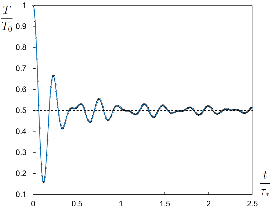
Figure 1: Short time behavior of kinetic temperature in the uniformly heated stretched square lattice. Solid line — analytical solution (58), dashed line — $T_{S}=T_{0}/2$, circles — numerical solution of lattice dynamics equations (55).

Figure 1 shows that analytical solution (58) coincides with results of numerical solution of lattice dynamics equations (55).

Temperature oscillations caused by equilibration of kinetic and potential energies decays in time. Characteristic time of the decay is of order of several periods $\tau_{*}$. Multiplying the temperature by time it can be shown that deviation from the stationary value decays as $1/t$. The same process in one-dimensional chain decays as $1/\sqrt{t}$. Heat propagation is a much slower process. For example, during $\tau_{*}$ the heat front passes the distance equal to $2\pi a$, which is small from macroscopic point of view.

Thus the example considered in the present section shows that oscillations of temperature and ballistic heat transfer have different time scales. Therefore the notions “fast process” and “slow process” are used. Comparison with results of computer simulations show that equation (58) accurately describe the fast process.

9.3 Ballistic heat transfer (slow process)

In the present section, we investigate the ballistic heat transfer described by formula (26) in the stretched square lattice.

9.3.1 Fundamental solution of the planar problem

We derive the fundamental solution of planar heat transport problem for the stretched square lattice. The following initial temperature distribution is considered:

$$T_{0}(x)=A\delta(x),$$ (59)

where $x$ is directed along the basis vector $\boldsymbol{\mathrm{a}}{}_{1}=a\boldsymbol{\mathrm{i}}{}$. Substituting the initial conditions into formula (43) and taking into account formula (56), yields:

$$T_{S}=\frac{A}{4\pi^{2}}\int_{0}^{\pi}\int_{0}^{\pi}\Bigl{(}\delta\left(x-c_{x}t\right)+\delta\left(x+c_{x}t\right)\Bigr{)}{\rm d}p_{1}{\rm d}p_{2},\qquad c_{x}=\frac{\displaystyle c_{*}\sin p_{1}}{\displaystyle 2\sqrt{\sin^{2}\frac{p_{1}}{2}+\sin^{2}\frac{p_{2}}{2}}}.$$ (60)

We make a substitution $\beta=\sin^{2}\frac{p_{1}}{2}$, $\gamma=\sin^{2}\frac{p_{2}}{2}$ and consider the case $t>0$, $x>0$. Solution for $x<0$ is obtained using symmetry of the problem. Then (60) takes the form:

$$T_{S}=\frac{A}{4\pi^{2}}\int_{0}^{1}\int_{0}^{1}\frac{\delta\left(\tilde{x}-\sqrt{\frac{\beta(1-\beta)}{\beta+\gamma}}\right)}{\sqrt{\beta\gamma(1-\beta)(1-\gamma)}}{\rm d}\beta{\rm d}\gamma,\qquad\tilde{x}=\frac{x}{c_{*}t}.$$ (61)

One of the integrals is evaluated using the identity (29). The argument of delta-function in formula (61) has roots given by the following equation

$$\gamma=\frac{\beta}{\tilde{x}^{2}}\left(1-\tilde{x}^{2}-\beta\right).$$ (62)

By the definition $0\leq\gamma\leq 1$. Then formula (62) yields the inequalities for $\beta$:

$$\beta\leq 1-\tilde{x}^{2},\qquad\beta^{2}-(1-\tilde{x}^{2})\beta+\tilde{x}^{2}\geq 0.$$ (63)

Solving the inequality (63) and using the identity (29), we obtain:

$$\begin{array}[]{l}\displaystyle T_{S}=\frac{A}{2\pi^{2}c_{*}t|\tilde{x}|}\begin{cases}\displaystyle f(0,1-\tilde{x}^{2}),\quad\sqrt{2}-1\leq|\tilde{x}|\leq 1,\\[11.38109pt] \displaystyle f(0,\beta_{1})+f(\beta_{2},1-\tilde{x}^{2}),\quad|\tilde{x}|\leq\sqrt{2}-1,\\[11.38109pt] \end{cases}\\[11.38109pt] \displaystyle\beta_{1,2}=\frac{1}{2}\left(1-\tilde{x}^{2}\mp\sqrt{(1-\tilde{x}^{2})^{2}-4\tilde{x}^{2}}\right),\\[11.38109pt] \displaystyle f(\xi_{1},\xi_{2})=\int_{\xi_{1}}^{\xi_{2}}\left(\frac{1-\beta}{(1-\tilde{x}^{2}-\beta)(\tilde{x}^{2}-\beta(1-\tilde{x}^{2}-\beta))}\right)^{\frac{1}{2}}{\rm d}\beta,\end{array}$$ (64)

and $T_{S}=0$ for $|\tilde{x}|\geq 1$. Formula (64) shows that function $T_{S}c_{*}t/A$ depends only on the self-similar variable $\tilde{x}$ (see figure 2).

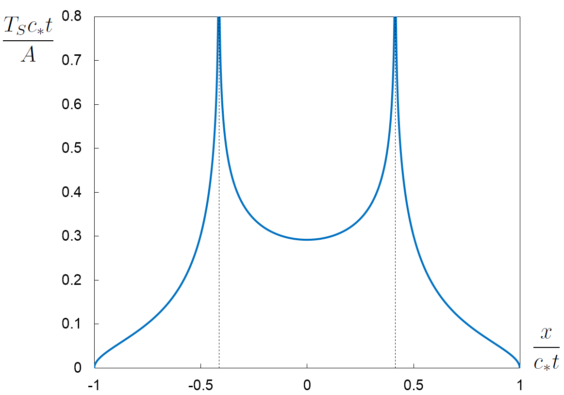
Figure 2: Solution of the heat transfer problem with initial conditions (59). Solid line — formula (64); dashed lines— vertical asymptotes at $|\tilde{x}|=\sqrt{2}-1$.

It is seen from figure 2 that the heat front moves with constant speed equal to $c_{*}$. Temperature have singularities at the points $|\tilde{x}|=\sqrt{2}-1$. Note that in one-dimensional chain the temperature in similar problem has singularities at the heat front $|\tilde{x}|=1$ (see formula (51)).

9.3.2 Thermal contact of hot and cold half-planes

Consider thermal contact of two half-planes with initial temperatures $T_{1}$ and $T_{2}$ (see formula (38)). This problem is important, because it is closely related to classical definition of temperature [38]. By the definition, temperatures of two bodies in thermodynamics equilibrium are equal. The problem considered below demonstrates the transition to thermodynamic equilibrium.

Substituting initial conditions (38) into the solution (43) and taking into account properties of the Heaviside function and function $c_{x}$, yields:

$$T_{S}=\frac{1}{4}\left(T_{1}+T_{2}\right)+\frac{1}{2}\left(T_{2}-T_{1}\right)w\left(\frac{|x|}{t}\right){\rm sign}\left(x\right),\qquad w=\frac{1}{2\pi^{2}}\int_{0}^{\pi}\int_{0}^{\pi}H\left(|x|-c_{x}t\right){\rm d}p_{1}{\rm d}p_{2}.$$ (65)

We make the substitution $\beta=\sin^{2}\frac{p_{1}}{2}$, $\gamma=\sin^{2}\frac{p_{2}}{2}$, then

$$w=\frac{1}{2\pi^{2}}\int_{0}^{1}\int_{0}^{1}\frac{H\left(|\tilde{x}|-\sqrt{\frac{\beta(1-\beta)}{\beta+\gamma}}\right)}{\sqrt{\beta\gamma(1-\beta)(1-\gamma)}}{\rm d}\beta{\rm d}\gamma.$$ (66)

Integrand in formula (66) is nonzero if the following inequality is satisfied:

$$\gamma\geq\frac{\beta}{\tilde{x}^{2}}\left(1-\tilde{x}^{2}-\beta\right).$$ (67)

The inequality (67) is satisfied identically for $\beta>1-\tilde{x}^{2}$; $\beta$ also satisfies the second inequality from (63). Then evaluation of the integral with respect to $\beta$, yields:

$$\begin{array}[]{l}\displaystyle w=\frac{1}{4}+\frac{1}{2\pi}\arcsin|\tilde{x}|-\begin{cases}g(0,1-\tilde{x}^{2}),~{}~{}\sqrt{2}-1\leq|\tilde{x}|\leq 1,\\[11.38109pt] \displaystyle\frac{\arcsin\beta_{2}-\arcsin\beta_{1}}{2\pi}+g(0,\beta_{1})+g(\beta_{2},1-\tilde{x}^{2}),~{}~{}|\tilde{x}|\leq\sqrt{2}-1,\\[11.38109pt] \end{cases}\\[11.38109pt] \displaystyle g(z_{1},z_{2})=\frac{1}{2\pi^{2}}\int_{z_{1}}^{z_{2}}\frac{\arcsin\left(\frac{2\beta}{\tilde{x}^{2}}\left(1-\tilde{x}^{2}-\beta\right)-1\right)}{\sqrt{\beta(1-\beta)}}{\rm d}\beta,\end{array}$$ (68)

where $\beta_{1},\beta_{2}$ are defined by formula (64); $w=\frac{1}{2}$ for $|\tilde{x}|\geq 1$.

Thus solution of the problem is given by formulas (65), (68). It is seen that the solution (68) is self-similar and it depends on $\tilde{x}=x/(c_{*}t)$.

We check the accuracy of formulas (65), (68) using numerical solution of lattice dynamics equations (55). Without loss of generality we put $T_{2}=2T_{1}$. In this case, initial conditions for particles has the form:

$$\begin{array}[]{l}u_{n,m}=0,\qquad v_{n,m}=\begin{cases}v_{0},\quad n<0,\\[11.38109pt] \sqrt{2}v_{0}\quad n>=0.\end{cases}\end{array}$$ (69)

where $v_{0}$ is a random quantity with dispersion $\Bigl{\langle}{v_{0}^{2}}\Bigr{\rangle}=k_{B}T_{1}/M$. Periodic boundary conditions are used. The periodic cell contains $4\cdot 10^{6}$ particles ($4\cdot 10^{2}$ in the $x$-direction and $10^{4}$ in the $y$-direction). In order to compute temperature, we consider $10^{3}$ realizations with initial conditions (69). Then temperature is computed by formula (8), where mathematical expectation is approximated by an average over realizations. Since the solution is self-similar, then it is sufficient to consider only one moment of time. Temperature distribution at $t=15\tau_{*}$ is computed. At this moment oscillations of kinetic temperature described in section 9.2 practically vanish. The temperature distribution is additionally averaged in $y$ direction. Comparison of numerical results with analytical solution (68) is shown in figure 3.

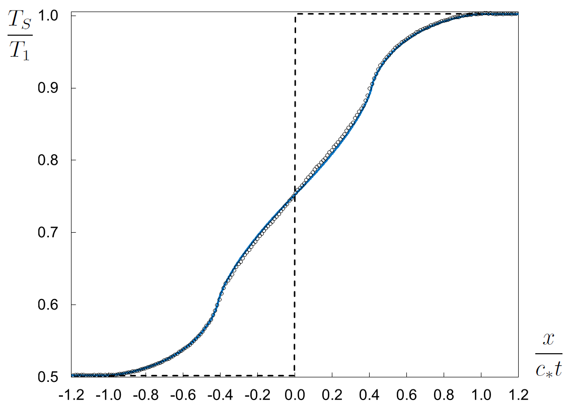
Figure 3: Contact of hot and cold half-planes: self-similar temperature profile. Line — analytical solution (68), circles — numerical solution of lattice dynamics equations (55).

Small differences between analytical and numerical solutions are observed in the vicinity of the central point $x=0$. At this point the temperature has large gradient (initially it is infinite) and therefore the long-wave approximation looses the accuracy. Far from the central point, analytical solution (68) almost coincide with numerical results.

9.3.3 Rectangular distribution of initial temperature. Thermal waves

In the present section, we demonstrate once again that the heat transfer in stretched square lattice is ballistic. Rectangular distribution of initial temperature is considered:

$$T_{0}(x)=2T_{1}\Bigl{(}H(x+L)-H(x-L)\Bigr{)},$$ (70)

where $L$ is a half-length of the interval with nonzero initial temperature. Solution of the problem with initial conditions (70) is obtained using formula (68) and the superposition principle. The resulting distribution of temperature at several moments of time is shown in figure 4.

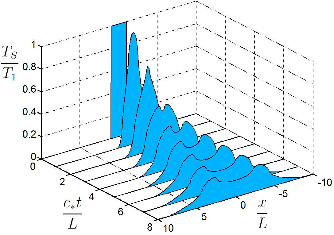
Figure 4: Evolution of rectangular initial temperature distribution (70) in scalar square lattice.

Figure 4 clearly shows two “thermal waves” traveling in opposite directions. Peaks of the temperature distribution move with constant speed equal to $(\sqrt{2}-1)c_{*}$. This fact can be used for validation of presented theory in future laboratory experiments.

9.3.4 Sinusoidal distribution of initial temperature

In the present section, we consider the decay of initial sinusoidal temperature distribution. This problem is important, because it allows to clearly demonstrate that the diffusive and hyperbolic [80, 81] heat transfer equations are not applicable to harmonic crystals. Similar problem for harmonic one-dimensional chains is considered in papers [71, 78, 79]. We also demonstrate the difference between time scales of fast and slow thermal processes.

Consider the following distribution of initial temperature:

$$T_{0}(x)=B_{0}\sin\frac{2\pi x}{L}+B_{1},$$ (71)

where $L$ is wave-length of initial temperature distribution; $B_{1}\geq B_{0}$. Fourier’s law as well as the hyperbolic heat transfer equation [80], [81] predict that amplitude of sin decays exponentially. In this section, we show using analytical solution (43) and numerical simulations that the amplitude decays inversely proportional to time.

Substituting the initial temperature distribution (71) into the general solution (43), yields:

$$\begin{array}[]{l}\displaystyle T=B(t)\sin\frac{2\pi x}{L}+B_{1},\qquad B(t)=B_{F}+B_{S},\\[11.38109pt] \displaystyle B_{F}=\frac{B_{0}}{2\pi^{2}}\int_{0}^{\pi}\int_{0}^{\pi}\cos\left(4\omega_{*}t\sqrt{\sin^{2}\frac{p_{1}}{2}+\sin^{2}\frac{p_{2}}{2}}\right){\rm d}p_{1}{\rm d}p_{2},\\[11.38109pt] \displaystyle B_{S}=\frac{B_{0}}{2\pi^{2}}\int_{0}^{\pi}\int_{0}^{\pi}\cos\left(\frac{\pi c_{*}t\sin p_{1}}{L\sqrt{\sin^{2}\frac{p_{1}}{2}+\sin^{2}\frac{p_{2}}{2}}}\right){\rm d}p_{1}{\rm d}p_{2}.\end{array}$$ (72)

Formula (72) contains two dimensionless times $\omega_{*}t$ and $c_{*}t/L$ corresponding to fast and slow thermal processes.

We check the accuracy of formula (72) using numerical solution of lattice dynamics equations (55). Particles have random initial velocities corresponding to initial temperature distribution (71). Initial particle displacements are equal to zero. Periodic boundary conditions in both directions are used. The periodic cell contains $2\cdot 10^{6}$ particles. The size of the periodic cell in the $x$-direction is equal to $L=2\cdot 10^{2}a$. Results are averaged over $10^{3}$ realizations with different initial conditions. The dependence of amplitude $B$ on dimensionless time $c_{*}t/L$ is shown in figure 5.

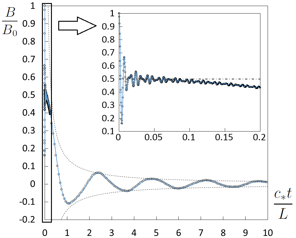
Figure 5: Decay of amplitude of initial sinusoidal temperature distribution (71). Short-time behavior of the amplitude is shown in the subplot. Solid line — analytical solution (72), circles — numerical solution of lattice dynamics equations (55), dashed lines — envelope $\pm 0.145L/(c_{*}t)$.

Every circle on the plot corresponds to average over realizations. Standard error of the mean is of order of the diameter of the circle. Figure 5 shows that analytical solution (72) practically coincides with results of numerical solution of lattice dynamics equations (55) at both short and large time scales.

The amplitude of sinusoidal distribution of initial temperature in scalar square lattice decays inversely proportional to time. In the one-dimensional chain with nearest neighbor interactions, the same oscillations are described by the Bessel function of the first kind [71, 78], which decays inversely proportional to square root of time. Therefore in both cases the amplitude decays according to a power law, while diffusive and hyperbolic [80, 81] heat transfer equations predict exponential decay.

This example also shows that the heat transfer process in scalar lattices is irreversible. At the same time, the general solution of the heat transfer problem (26) is symmetric with respect to time, i.e. invariant with respect to substitution $t$ by $-t$. This fact may serve for better understanding of the Loschmidt’s (reversibility) paradox [82].

9.3.5 Fundamental solution

The fundamental solution of heat transport problem for two-dimensional scalar lattices is given by formula (36). In order to obtain the solution for the square lattice, we calculate the Jacobian $G$ using formulas (36) and (56):

$$G=-\frac{c_{*}^{2}\left(\cos p_{1}\sin^{4}\frac{p_{2}}{2}+\cos p_{2}\sin^{4}\frac{p_{1}}{2}\right)}{4\left(\sin^{2}\frac{p_{1}}{2}+\sin^{2}\frac{p_{2}}{2}\right)^{2}}.$$ (73)

We make two consecutive substitutions in formulas (36), (73): $s_{1}=\sin^{2}\frac{p_{1}}{2},s_{2}=\sin^{2}\frac{p_{2}}{2}$ and $w=s_{1}s_{2}$, $q=s_{1}+s_{2}$. Then excluding $w$ we obtain:

$$\begin{array}[]{l}\displaystyle T_{S}=\frac{A}{2(\pi c_{*}t)^{2}}\sum_{j}\frac{q_{j}}{|q_{j}^{2}-\tilde{r}^{2}(q_{j}+1)|},\\[14.22636pt] \displaystyle q_{j}^{3}-2\left(\tilde{r}^{2}+1\right)q_{j}^{2}+\bigl{(}(\tilde{r}^{2}+1)^{2}-4\tilde{x}^{2}\tilde{y}^{2}+1\bigr{)}q_{j}-2\tilde{r}^{2}=0,\end{array}$$ (74)

where $\tilde{r}^{2}=1-\tilde{x}^{2}-\tilde{y}^{2}$, $\tilde{x}=\frac{x}{c_{*}t}$, $\tilde{y}=\frac{y}{c_{*}t}$. Summation is carried out with respect to all real roots $q_{j}$ of the given cubic equation such that $q_{j}\in[0;2]$. Formula (74) shows that the function $Tc_{*}^{2}t^{2}/A$ is self-similar.

Formula (74) gives closed-form fundamental solution for harmonic scalar square lattice. According to formula (74), the temperature is nonzero inside the circle $\tilde{x}^{2}+\tilde{y}^{2}\leq 1$. It has singularity along the line determined by the following system of equations:

$$\tilde{x}^{2}+\tilde{y}^{2}=1-\frac{q^{2}}{q+1},\qquad\tilde{x}^{2}\tilde{y}^{2}=\frac{2-q^{2}}{4(q+1)^{2}}.$$ (75)

The line (75) is shown in figure 6. It intersects $\tilde{x}$-axis at the points $\pm(\sqrt{2}-1)$.

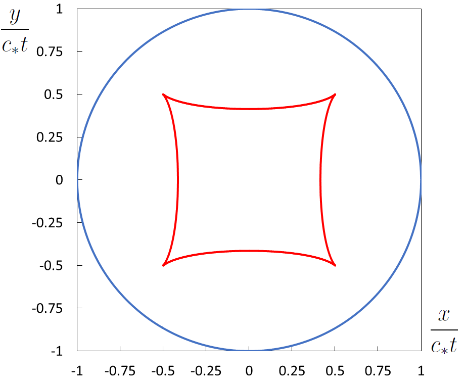
Figure 6: Heat front (circle) and line with infinite temperature (equation (75)) corresponding to the fundamental solution (74).

Fundamental solution (74) is symmetrical with respect to axes $\tilde{x}$ and $\tilde{y}$. Solution for positive $\tilde{x}$, $\tilde{y}$ is shown in figure 7.

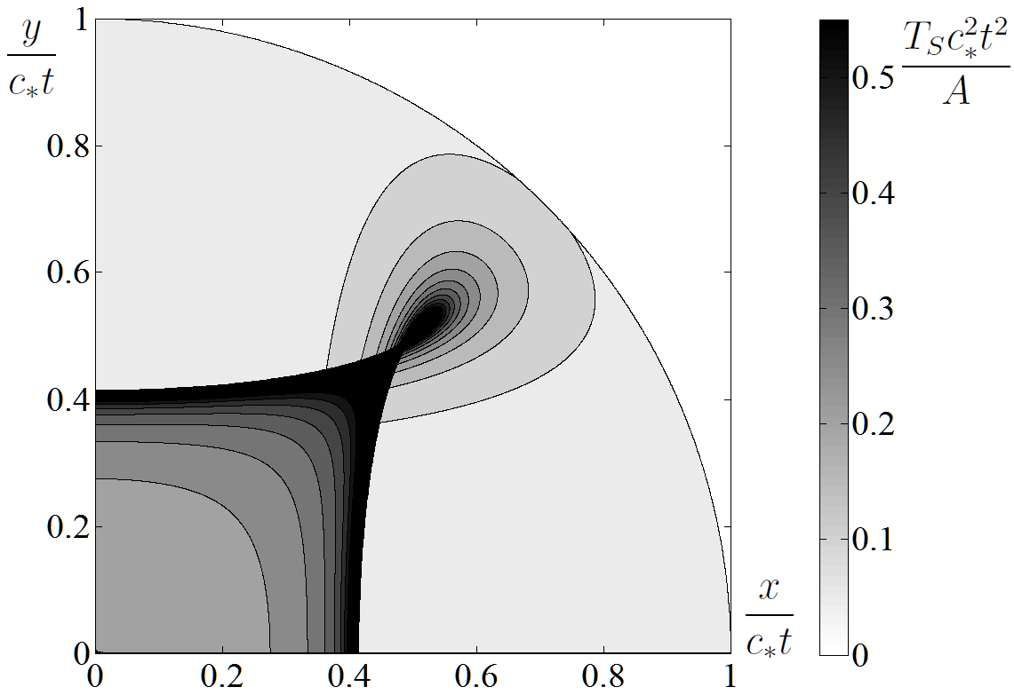
Figure 7: Fundamental solution (74) of the unsteady heat transfer problem for scalar square lattice.

We check the accuracy of fundamental solution (74) as follows. Problems described in sections 9.3.1, 9.3.2 are solved using the convolution of the fundamental solution with corresponding initial conditions. It is shown that the resulting temperature distribution coincides with results obtained in sections 9.3.1, 9.3.2.

Thus the closed-form fundamental solution of unsteady heat transfer problem for scalar square lattice is given by formula (74). We note the analogy between our result (74) and results obtained in papers [42, 45]. In papers [42, 45], spatial distribution of energy corresponding to the fundamental solution of equations of motion (2) is obtained using the Wigner transform. The energy distribution is similar to temperature distribution shown in figure 7. Therefore there is an analogy between deterministic lattice dynamics problem [42] and the unsteady heat transfer problem discussed above.

10 Conclusions

An equation exactly describing the evolution of temperature field in any scalar lattice was derived. Using this equation, we have shown that the temperature field in a lattice with random initial velocities and zero initial displacements is represented as a sum of two terms (see formulas (24), (25), (26)).

The first term describes short time behavior of temperature. At short times, temperature performs decaying oscillations caused by redistribution of energy among kinetic and potential forms. These oscillations in different spatial point are independent. Characteristic time of decay is of order of ten periods of atomic vibrations.

The second term describes large time behavior of kinetic temperature associated with unsteady ballistic heat transfer. At large times, the temperature field is represented as a superposition of waves having a shape of initial temperature distribution and traveling with the group velocity. The heat front propagates with constant speed equal to the maximum group velocity. These observations are consistent with results obtained in papers [42, 43, 44, 45, 46] by completely different means. Closed-form fundamental solutions of the unsteady heat transfer problem for one- and two-dimensional scalar lattices were derived.

The expression for the temperature field has the same property as the equations of motions: it is invariant to the substitution $t\rightarrow-t$. However thermal processes in scalar lattices are irreversible. In order to illustrate this fact, an analytical solution for problem with sinusoidal distributions of initial temperature in scalar square lattice was derived. The solution shows that the amplitude of sinusoidal distribution decays inversely proportional to time. Therefore the process is irreversible, while it is described by the equation invariant to the substitution $t\rightarrow-t$.

Comparison of analytical results with numerical simulations shows that presented theory describes the behavior of temperature field at both short and large time scales with high accuracy.

11 Acknowledgements

The authors are deeply grateful to M.B. Babenkov, W.G. Hoover, S.N. Gavrilov, E.A. Ivanova, D.A. Indeytsev, M.L. Kachanov, O.S. Loboda, G.S. Mishuris, N.F. Morozov, and A. Politi for useful discussions. Comments of the reviewers are highly appreciated.

Numerical simulations have been carried out using facilities of the Supercomputer Center “Polytechnic” at Peter the Great Saint Petersburg Polytechnic University.

This work was supported by the Russian Science Foundation (RSCF grant No. 17-71-10213).

Appendix A Appendix. Equations for covariances

In the present appendix, we derive equation (9) for velocity covariances. Note that particle velocities satisfy equation of motion (2):

$$\ddot{v}\left(\boldsymbol{\mathrm{x}}{}\right)={\cal L}v\left(\boldsymbol{\mathrm{x}}{}\right).$$ (76)

We introduce covariance of accelerations

$$\zeta=\Bigl{\langle}{\dot{v}(\boldsymbol{\mathrm{x}}{})\dot{v}(\boldsymbol{\mathrm{y}}{})}\Bigr{\rangle}.$$ (77)

Differentiating covariances of velocities $\kappa$ and covariances of accelerations $\zeta$ with respect to time and taking into account equations of motion (2), (76), yields:

$$\ddot{\kappa}=\left({\cal L}_{x}+{\cal L}_{y}\right)\kappa+2\zeta,\quad\ddot{\zeta}=\left({\cal L}_{x}+{\cal L}_{y}\right)\zeta+2{\cal L}_{x}{\cal L}_{y}\kappa.$$ (78)

Excluding $\zeta$ from system (78) yields equation (9) for velocity covariances.

Appendix B Appendix. Approximation of difference operators

In the present appendix, we describe series expansion of difference operators ${\cal L}_{x}$, ${\cal L}_{y}$. We represent the covariance of particle velocities in the form $\kappa\left(\boldsymbol{\mathrm{r}}{},\boldsymbol{\mathrm{x}}{}-\boldsymbol{\mathrm{y}}{}\right)$ (see formula (12)). Consider the following expression

$$\begin{array}[]{l}\displaystyle{\cal L}_{x}\kappa\left(\boldsymbol{\mathrm{r}}{},\boldsymbol{\mathrm{x}}{}-\boldsymbol{\mathrm{y}}{}\right)=\omega_{*}^{2}\sum_{\alpha}b_{\alpha}\kappa\left(\boldsymbol{\mathrm{r}}{}+\frac{1}{2}\boldsymbol{\mathrm{a}}{}_{\alpha},\boldsymbol{\mathrm{x}}{}-\boldsymbol{\mathrm{y}}{}+\boldsymbol{\mathrm{a}}{}_{\alpha}\right).\end{array}$$ (79)

Assume that function $\kappa$ slowly changes with the first argument at distances of order of $|\boldsymbol{\mathrm{a}}{}_{\alpha}|$. Then series expansion in the right side of formula (79) with respect to $\boldsymbol{\mathrm{a}}{}_{\alpha}$ yields

$$\begin{array}[]{l}\displaystyle{\cal L}_{x}\kappa\approx\omega_{*}^{2}\sum_{\alpha}b_{\alpha}{\cal S}_{\alpha}\kappa+\frac{\omega_{*}^{2}}{2}\sum_{\alpha}b_{\alpha}{\cal S}_{\alpha}\boldsymbol{\mathrm{a}}{}_{\alpha}\cdot\nabla\kappa=\left({\cal L}+\boldsymbol{\mathrm{{\cal R}}}{}\cdot\nabla\right)\kappa,\\[11.38109pt] \displaystyle\boldsymbol{\mathrm{{\cal R}}}{}=\frac{\omega_{*}^{2}}{2}\sum_{\alpha}b_{\alpha}{\cal S}_{\alpha}\boldsymbol{\mathrm{a}}{}_{\alpha},\qquad{\cal L}=\omega_{*}^{2}\sum_{\alpha}b_{\alpha}{\cal S}_{\alpha},\qquad{\cal S}_{\alpha}\kappa=\kappa\left(\boldsymbol{\mathrm{r}}{},\boldsymbol{\mathrm{x}}{}-\boldsymbol{\mathrm{y}}{}+\boldsymbol{\mathrm{a}}{}_{\alpha}\right),\end{array}$$ (80)

where $\nabla=\frac{\partial}{\partial\boldsymbol{\mathrm{r}}{}}$ is nabla-operator. Formulas (80) yield ${\cal L}_{x}\approx{\cal L}+\boldsymbol{\mathrm{{\cal R}}}{}\cdot\nabla$. Analogously we show that ${\cal L}_{y}\approx{\cal L}-\boldsymbol{\mathrm{{\cal R}}}{}\cdot\nabla$. Then

$${\cal L}_{x}-{\cal L}_{y}\approx 2\boldsymbol{\mathrm{{\cal R}}}{}\cdot\nabla,\qquad{\cal L}_{x}+{\cal L}_{y}\approx 2{\cal L}.$$ (81)

Substitution of the expressions (81) into equation (9), yields formula (14).

Appendix C Appendix. Group velocity

In this appendix, we prove that $\boldsymbol{\mathrm{c}}{}$, defined by formula (20), coincides with the group velocity for the lattice.

The discrete Fourier transform in $d$-dimensional space for an infinite lattice is defined as follows

$$\begin{array}[]{l}\displaystyle\hat{\kappa}\left(\boldsymbol{\mathrm{k}}{}\right)=\Phi\left(\kappa\right)=\sum_{j=1}^{d}\sum_{z_{j}=-\infty}^{+\infty}\kappa(\boldsymbol{\mathrm{z}}{})e^{-i\boldsymbol{\mathrm{k}}{}\cdot\boldsymbol{\mathrm{z}}{}},\qquad\displaystyle\kappa(\boldsymbol{\mathrm{z}}{})=\frac{1}{(2\pi)^{d}}\int_{-\pi}^{\pi}\hat{\kappa}(\boldsymbol{\mathrm{k}}{})e^{i\boldsymbol{\mathrm{k}}{}\cdot\boldsymbol{\mathrm{z}}{}}{\rm d}p_{1}...{\rm d}p_{d},\\[11.38109pt] \displaystyle\boldsymbol{\mathrm{k}}{}=\frac{1}{a}\sum_{j=1}^{d}p_{j}\tilde{\boldsymbol{\mathrm{e}}{}}_{j},\quad\boldsymbol{\mathrm{z}}{}=\boldsymbol{\mathrm{x}}{}-\boldsymbol{\mathrm{y}}{}=a\sum_{j=1}^{d}z_{j}\boldsymbol{\mathrm{e}}{}_{j},\quad\boldsymbol{\mathrm{e}}{}_{j}\cdot\tilde{\boldsymbol{\mathrm{e}}{}}_{k}=\delta_{jk}.\end{array}$$ (82)

Here $a$ is equilibrium distance, $i$ is the imaginary unit, $\boldsymbol{\mathrm{e}}{}_{j}$ are basis vectors for the lattice, $\tilde{\boldsymbol{\mathrm{e}}{}}_{k}$ are vectors of the reciprocal basis, $\delta_{jk}$ is the Kronecker delta. The discrete Fourier transform has the following property:

$$\Phi\left(\kappa(\boldsymbol{\mathrm{z}}{}+\boldsymbol{\mathrm{a}}{}_{\alpha})\right)=\Phi\left(\kappa(\boldsymbol{\mathrm{z}}{})\right)e^{i\boldsymbol{\mathrm{k}}{}\cdot\boldsymbol{\mathrm{a}}{}_{\alpha}}.$$ (83)

Using the identity (83), we show that

$$\begin{array}[]{l}\displaystyle\Phi\left({\cal L}\kappa\right)=\hat{{\cal L}}\hat{\kappa},\qquad\hat{{\cal L}}=\omega_{*}^{2}\sum_{\alpha}b_{\alpha}e^{i\boldsymbol{\mathrm{k}}{}\cdot\boldsymbol{\mathrm{a}}{}_{\alpha}},\qquad\displaystyle\Phi\left(\boldsymbol{\mathrm{{\cal R}}}{}\kappa\right)=\hat{\boldsymbol{\mathrm{{\cal R}}}{}}\hat{\kappa},\qquad\hat{\boldsymbol{\mathrm{{\cal R}}}{}}=\frac{\omega_{*}^{2}}{2}\sum_{\alpha}b_{\alpha}\boldsymbol{\mathrm{a}}{}_{\alpha}e^{i\boldsymbol{\mathrm{k}}{}\cdot\boldsymbol{\mathrm{a}}{}_{\alpha}}.\end{array}$$ (84)

Consider the discrete Fourier transform of equation (14). Calculating the transform using identities (84), we obtain

$$\ddddot{\hat{\kappa}}-4\hat{{\cal L}}\ddot{\hat{\kappa}}+4\left(\hat{\boldsymbol{\mathrm{{\cal R}}}{}}\cdot\nabla\right)^{2}\hat{\kappa}=0.$$ (85)

Then vector $\boldsymbol{\mathrm{c}}{}$ is introduced as

$$\boldsymbol{\mathrm{c}}{}=\frac{{\rm Im}\hat{\boldsymbol{\mathrm{{\cal R}}}{}}}{\sqrt{-\hat{{\cal L}}}}.$$ (86)

It can be shown that $\hat{{\cal L}}$ and $\hat{\boldsymbol{\mathrm{{\cal R}}}{}}$ are related by the following formula:

$$\hat{\boldsymbol{\mathrm{{\cal R}}}{}}=-\frac{i}{2}\frac{{\rm d}\hat{{\cal L}}}{{\rm d}\boldsymbol{\mathrm{k}}{}}.$$ (87)

Substituting formula (87) into formula (86), we obtain

$$\boldsymbol{\mathrm{c}}{}=\frac{{\rm d}\sqrt{-\hat{{\cal L}}}}{{\rm d}\boldsymbol{\mathrm{k}}{}}.$$ (88)

Consider the dispersion relation for the lattice. Substituting $u(\boldsymbol{\mathrm{x}}{})=A\exp(i(\omega t+\boldsymbol{\mathrm{k}}{}\cdot\boldsymbol{\mathrm{x}}{}))$ into the equation of motion (2), yields:

$$\omega^{2}=-\omega_{*}^{2}\sum_{\alpha}b_{\alpha}e^{i\boldsymbol{\mathrm{k}}{}\cdot\boldsymbol{\mathrm{a}}{}_{\alpha}}=-\hat{{\cal L}}.$$ (89)

Combining the dispersion relation (89) with formulas (84), (88), yields

$$\boldsymbol{\mathrm{c}}{}=\frac{{\rm d}\omega}{{\rm d}\boldsymbol{\mathrm{k}}{}}.$$ (90)

Therefore, $\boldsymbol{\mathrm{c}}{}$ is equal to the group velocity.

References

- [1] R.E. Peierls, Quantum theory of solids (Oxford University Press, 1965), p. 238.
- [2] J.M. Ziman, Electrons and Phonons. The theory of transport phenomena in solids. (Oxford University Press, New York, 1960), p. 554.
- [3] T.K. Hsiao, H.K. Chang, S.-C. Liou, M.-W. Chu, S.-C. Lee, C.-W. Chang, Nat. Nanotech., 8(7), 534 (2013).
- [4] D.G. Cahill, W.K. Ford, K.E. Goodson, G.D. Mahan, A. Majumdar, H.J. Maris, R. Merlin, S.R. Phillpot, J. Appl. Phys. 93, 793 (2003).
- [5] S. Liu, X.F. Xu, R.G. Xie, G. Zhang, B.W. Li, Eur. Phys. J. B, 85, 337 (2012).
- [6] C.W. Chang, in: Thermal transport in low dimensions, Lecture Notes in Physics, Vol. 921, 2016, pp. 305-338.
- [7] T.Y. Chen, C.L. Chien, M. Manno, L. Wang, C. Leighton, Phys. Rev. B 81, 020301 (2010).
- [8] M.E. Pumarol, M.C. Rosamond, P. Tovee, M.C. Petty, D.A. Zeze, V. Falko, O.V. Kolosov, Nano Lett., 12 (6), 2906 (2012).
- [9] A. Cenian, H. Gabriel J. Phys.: Condens. Matter, 13, 4323 (2001).
- [10] L. Shi, et.al. Nanoscale and Microscale Thermophysical Engineering, 19, 127 (2015).
- [11] F. Bonetto, J.L. Lebowitz, L. Rey-Bellet, In: Mathematical Physics, Imperial College Press, London, 2000.
- [12] Z. Rieder, J.L. Lebowitz, E. Lieb, J. Math. Phys. 8, 1073 (1967).
- [13] K.R. Allen, J. Ford, Phys. Rev., 187, 1132 (1969).
- [14] H. Nakazawa, Progr. Phys., 45, 231 (1970).
- [15] V. Kannan, A. Dhar, J.L. Lebowitz , Phys. Rev. E, 85, 041118 (2012).
- [16] L.W. Lee, A. Dhar, Phys. Rev. Lett. 95(9), 094302 (2005).
- [17] A. Kundu, A. Chaudhuri, D. Roy, A. Dhar, J.L. Lebowitz, H. Spohn, EPL, 90(4), 40001 (2010).
- [18] I.F. Herrera-Gonzalez, F.M. Izrailev, L. Tessieri, EPL, 90, 14001 (2010).
- [19] I.F. Herrera-Gonzalez, F.M. Izrailev, L. Tessieri, EPL, 110, 64001 (2015).
- [20] S. Lepri, C. Mejia-Monasterio, A. Politi, J. Phys. A: Math., Theor. 42, 025001 (2009).
- [21] S. Lepri, C. Mejia-Monasterio, A. Politi, J. Phys. A: Math., Theor. 43, 065002 (2010).
- [22] A. Dhar, K. Venkateshan, J.L. Lebowitz, Phys. Rev. E, 83, 021108 (2011).
- [23] C. Bernardin, V. Kannan, J.L. Lebowitz, J. Lukkarinen, J. Stat. Phys., 146(4), 800 (2012).
- [24] N. Freitas, J.P. Paz, Phys. Rev. E, 90, 042128 (2014).
- [25] A. Dhar, K. Saito, in: Thermal transport in low dimensions, Lecture Notes in Physics, Vol. 921, pp. 305-338 (2016).
- [26] S. Lepri, R. Livi, A. Politi, Phys. Rep. 377, 1 (2003).
- [27] F. Bonetto, J.L. Lebowitz, J. Lukkarinen, J. Stat. Phys., 116, 783 (2004).
- [28] W.G. Hoover, C.G. Hoover, Commun. Nonlinear Sci. Numer. Simulat. 18, 3365 (2013).
- [29] M.P. Allen and D.J. Tildesley, Computer Simulation of Liquids, (Clarendon Press, Oxford, 1987), p. 385.
- [30] D.H. Tsai, R.A. MacDonald, Phys. Rev. B, 14(10), 4714 (1976).
- [31] A.J.C. Ladd, B. Moran, W.G. Hoover, Phys. Rev. B, 34, 5058 (1986).
- [32] A.A. Selezenev, A.Yu. Aleinikov, N.S. Ganchuk, S.N. Ganchuk, R.E. Jones, J.A. Zimmerman, Phys. Solid State, 55, 889 (2013).
- [33] X.W. Zhou, S. Aubry, R.E. Jones, A. Greenstein, P.K. Schelling, Phys. Rev. B, 79 115201 (2009).
- [34] O.V. Gendelman, A.V. Savin, Phys. Rev. E, 81, 020103, (2010).
- [35] A.A. Le-Zakharov, A.M. Krivtsov, Dokl. Phys., 53, 261 (2008).
- [36] Y.A. Kosevich, A.V. Savin, Phys. Lett. A, 380, 3480 (2016).
- [37] F. Piazza, S. Lepri, Phys. Rev. B, 79, 094306 (2009).
- [38] W.G. Hoover, Computational statistical mechanics, (Elsevier, N.Y., 1991). p. 330.
- [39] A.M. Krivtsov, Dokl. Phys. 59(9), (2014).
- [40] M.B. Babenkov, A.M. Krivtsov, D.V. Tsvetkov. Phys. Mesomech., 19(3), 282 (2016).
- [41] V.A. Kuzkin, A.M. Krivtsov, Phys. Solid State, 59(5), 1051 (2017).
- [42] A. Mielke, Arch. Ration. Mech. Anal., 181, 401 (2006).
- [43] J. Lukkarinen, H. Spohn, Arch. Rat. Mech. Anal. 183 (1), 93 (2007).
- [44] T.V. Dudnikova, H. Spohn, Markov Processes and Related Fields, 12(4), 645 (2006).
- [45] L. Harris, J. Lukkarinen, S. Teufel, F. Theil, SIAM J. Math. Anal., 40(4) 1392 (2008).
- [46] J. Lukkarinen, M. Marcozzi, A. Nota, J. Stat. Phys. 165, 809 (2016).
- [47] P.B. Corkum, F. Krausz, Nat. Phys. 3, 381 (2007).
- [48] N.A. Inogamov, Yu.V. Petrov, V.V. Zhakhovsky, V.A. Khokhlov, B.J. Demaske, S.I. Ashitkov, K.V. Khishchenko, K.P. Migdal, M.B. Agranat, S.I. Anisimov, V.E. Fortov, I.I. Oleynik. AIP Conf. Proc. 1464, 593 (2012).
- [49] K.V. Poletkin, G.G. Gurzadyan, J. Shang, V. Kulish, App. Phys. B, 107, 137 (2012).
- [50] A.A. Balandin, Nat. Mat. 10 (2011).
- [51] A.V. Savin, V. Zolotarevskiy, O.V. Gendelman, EPL, 113, 24003 (2016).
- [52] N. Nishiguchi, Y. Kawada, E. Sakuma, J. Phys: Condens. Matter, 4, 10227 (1992).
- [53] G.S. Mishuris, A.B. Movchan, L.I. Slepyan, J. Mech. Phys. Sol. 57, 1958 (2009).
- [54] Z. Liu, B. Li, , J. Phys. Soc. Jap. 77, (2008).
- [55] V.A. Kuzkin, A.M. Krivtsov, Phys. Stat. Sol. b, 252, 1664 (2015).
- [56] J.-S. Wang, B. Li, Phys. Rev. E, 70, 021204 (2004).
- [57] V.A. Kuzkin, Phys. Rev. E, 82, 016704 (2010).
- [58] T. Zhu, E. Ertekin, Nano Lett., 16, 4763 (2016).
- [59] D.L. Nika, A.A. Balandin, Rep. Prog. Phys. 80 036502 (2017).
- [60] Z.-X. Xie, K.-Q. Chen, W. Duan, J. Phys.: Condens. Matter, 23, 315302 (2011).
- [61] I.E. Berinskii, D.A. Indeitsev, N.F. Morozov, D.Yu. Skubov, L.V. Shtukin, Mech. Solids, 50(2), 127 (2015).
- [62] T. Zhu, E. Ertekin, Phys. Rev. B 90, 195209 (2014).
- [63] I.E. Berinskii, A.Yu. Panchenko, E.A. Podolskaya, Model. Simul. Mat. Sci. and Eng. 24(4) (2016).
- [64] B. Liu, F. Meng, C.D. Reddy, J.A. Baimova, N. Srikanth, S.V. Dmitriev, K. Zhou, RSC Adv. 5, 29193 (2015).
- [65] V.A. Kuzkin, I.E. Asonov, Phys. Rev. E. 86, 051301 (2012).
- [66] M.J. Nieves, A.B. Movchan, I.S. Jones, G.S. Mishuris, J. Mech. Phys. Sol. 61 (6), 1464 (2013).
- [67] D.A. Indeitsev, A.D. Sergeev, Vestnik St. Petersburg University, Mathematics, 50 (2), 166 (2017).
- [68] T.V. Dudnikova, A.I. Komech, H. Spohn, J. Math. Phys., 44, 2596 (2003).
- [69] T.V. Dudnikova, A.I. Komech, N.J. Mauser, J. Stat. Phys., 114(3/4), 1035 (2004).
- [70] V.V. Kozlov, D.V. Treschev, J. Math. Sci. 128, 2791 (2005).
- [71] A.M. Krivtsov, Dokl. Phys. 60(9), 407 (2015).
- [72] M. Born, K. Huang, Dynamical theory of crystal lattices (Clarendon Press, Oxford, 1954).
- [73] R. Wong, Asymptotic approximations of Integrals, (Academic Press, 1989), p. 556.
- [74] H. Spohn, J. Stat. Phys., 124 (2-4), 1041 (2006).
- [75] H. Spohn, J.L. Lebowitz, Commun. math. Phys. 54, 97 (1977).
- [76] I. M. Gel’fand, G. E. Shilov, Generalized functions. Volume I: Properties and operations, (Academic Press, 1964), p. 423.
- [77] B. Li, J. Wang, Phys. Rev. Lett., 91(4) 044301 (2003).
- [78] A.M. Krivtsov. ArXiv:1509.02506 [cond-mat.stat-mech], (2015).
- [79] O.V. Gendelman, R. Shvartsman, B. Madar, A.V. Savin, Phys. Rev. E, 85(1), 011105 (2012).
- [80] C. Cattaneo, Comptes rendus de l Academie des sciences, 247, 431 (1958).
- [81] P. Vernotte, Comptes rendus de l Academie des sciences, 246, 3154 (1958).
- [82] W.G. Hoover, C.G. Hoover, Time reversibility, computer simulation, algorithms, chaos. Advanced Series in Nonlinear Dynamics Vol. 13, (World Scientific, 2013), p. 428.