Geometric phase of a moving dipole under a magnetic field at a distance

Abstract

We predict a geometric quantum phase shift of a moving electric dipole in the presence of an external magnetic field at a distance. On the basis of the Lorentz-covariant field interaction approach, we show that a geometric phase appears under the condition that the dipole is moving in the field-free region, which is distinct from the topological He-McKellar-Wilkens phase generated by a direct overlap of the dipole and the field. We discuss the experimental feasibility of detecting this phase with atomic interferometry and argue that detection of this phase would result in a deeper understanding of the locality in quantum electromagnetic interaction.

Introduction.- A moving charge under an external electric/magnetic field exhibits a topological quantum phase shift known as the Aharonov-Bohm (AB) effect Aharonov and Bohm (1959). An intriguing aspect of the AB effect is that it takes place even without a local overlap between the charge and the external field (see Ref. Peshkin and Tonomura, 1989 for a review). A similar topological phase shift, namely the He-McKellar-Wilkens (HMW) phase He and McKellar (1993); Wilkens (1994), was predicted for an electric dipole under an external magnetic field. The HMW phase shift is given by

$$\Delta\phi_{HMW}=\frac{1}{\hbar c}\oint\mathbf{B}\times\mathbf{d}\cdot d\mathbf{R}$$ (1)

for a closed path $\mathbf{R}$ of the dipole, where $\mathbf{B}$ and $\mathbf{d}$ are the external magnetic field and the dipole moment, respectively. This phase can be derived from the interaction Lagrangian of a moving dipole under a magnetic field, introduced by Wilkens Wilkens (1994):

$$L_{W}=\frac{1}{c}\mathbf{d}\cdot(\dot{\mathbf{R}}\times\mathbf{B})\,.$$ (2)

Despite their similarity, there is a notable difference between the HMW and the AB phases. For an observation of the HMW phase, the moving particle should experience a direct overlap with the external magnetic field. In contrast, the AB phase shift can be generated without a direct overlap of the interfering particle and the external field. An interesting question here is whether any measurable result arises from the interaction between a dipole and the external field without a direct overlap of the two entities. As far as the topological phase is concerned, no measurable effect is produced between the nonoverlapping $\mathbf{d}$ and $\mathbf{B}$, which is apparent from Eqs. (1) and (2). This point was addressed in Refs. Spavieri, 1998 and Wilkens, 1998.

In this Letter, we predict a novel quantum phase shift of a moving dipole under a magnetic field in the absence of a direct overlap of the two entities. Our prediction is based on the Lorentz-covariant field-interaction (LCFI) approach Kang (2013, 2015a). The essence of the LCFI theory is that, the effect of an external electromagnetic field on a moving charge can be universally represented by the interaction between the two electromagnetic fields, the external field and that generated by the charge, along with the incorporation of the relativity principle. The electromagnetic potential is eliminated accordingly. It was demonstrated that the LCFI approach reproduces the established result for the topological AB effect. In addition, this theory leads to the prediction of a new type of quantum interference that cannot be described in the standard potential-based theory Kang (2015b). Here, on the basis of the LCFI framework, we find a non-topological geometric quantum phase of a moving dipole in the absence of the local overlap of $\mathbf{d}$ and $\mathbf{B}$. We also propose a realistic setup for observing this phase with a hydrogenlike atom under a distant semi-infinite magnetic sheet. Notably, this geometric phase cannot be predicted with either the Wilkens’ (Eq. (2)) or the standard potential-based approaches. This implies that a successful experiment would shed light on our understanding of the quantum locality and the role of potential in the electromagnetic interaction.

Lagrangian and Hamiltonian for an electric dipole.- In the LCFI approach, the influence of the external electric ($\mathbf{E}$) and magnetic ($\mathbf{B}$) fields on a moving charge $q$ is described by the Lorentz-covariant interaction Lagrangian Kang (2013, 2015a)

$$L_{int}^{q}=\frac{1}{4\pi}\int(\mathbf{B}_{q}\cdot\mathbf{B}-\mathbf{E}_{q}\cdot\mathbf{E})d^{3}\mathbf{r}^{\prime}\,,$$ (3)

where $\mathbf{E}_{q}$($\mathbf{B}_{q}$) represents the electric(magnetic) field generated by the charge $q$. It was previously shown that this Lagrangian reproduces the force-free topological AB effect, which is equivalent to the well established result obtained from the potential-based theory Kang (2013, 2015a). This demonstrates the validity of the field-interaction framework. Here, we deal with the quantum effect generated by the external $\mathbf{B}$ and drop the second term in the right-hand side of Eq. (3) not . Eq. (3) can then be rewritten as

$$L_{int}^{q}=\dot{\mathbf{r}}\cdot\mathbf{\Pi}_{q}\,,$$ (4a)

where $$\dot{\mathbf{r}} q$$ is the velocity of charge and

$$\mathbf{\Pi}_{q}=\frac{1}{4\pi c}\int\mathbf{E}_{q}\times\mathbf{B}\ d^{3}\mathbf{r}^{\prime}$$ (4b)

is the field momentum produced by the overlap between $\mathbf{E}_{q}$ and $\mathbf{B}$.

The LCFI approach is not limited to a single point charge and can be generalized to an arbitrary distribution of charges. We adopt it for describing the interaction between the dipole and the external field. Applying Eq. (4), the interaction between an electric dipole (composed of two point charges $q$ and $-q$) and $\mathbf{B}$ is described by the interaction Lagrangian

$$L_{int}=\dot{\mathbf{r}}_{q}\cdot\mathbf{\Pi}_{q}(\mathbf{r}_{q})+\dot{\mathbf{r}}_{\bar{q}}\cdot\mathbf{\Pi}_{\bar{q}}(\mathbf{r}_{\bar{q}})\,,$$ (5)

where $\mathbf{r}_{q}$($\mathbf{r}_{\bar{q}}$) and $\mathbf{\Pi}_{q}$($\mathbf{\Pi}_{\bar{q}}$) are the position of charge $q$ ($-q$) and the corresponding field momentum defined in Eq. (4b), respectively. Applying the dipole approximation

$$\mathbf{\Pi}_{q}(\mathbf{r}_{q})\simeq\mathbf{\Pi}_{q}(\mathbf{R})+(\mathbf{r}_{q}-\mathbf{R})\cdot\nabla\mathbf{\Pi}_{q}(\mathbf{R}),$$

we find

$$L_{int}=\dot{\mathbf{R}}\cdot(\mathbf{r}\cdot\nabla)\mathbf{\Pi_{q}}(\mathbf{R})+\dot{\mathbf{r}}\cdot\mathbf{\Pi_{q}}(\mathbf{R}),$$ (6)

where $\mathbf{R}$ and $\mathbf{r}\equiv\mathbf{r}_{q}-\mathbf{r}_{\bar{q}}$ are the center of mass and the relative coordinates of the two charges, respectively. Here the gradient $\nabla$ is associated with the $\mathbf{R}$ coordinates; that is, $\nabla\equiv\nabla_{\mathbf{R}}$.

The field momentum $\mathbf{\Pi_{q}}$ satisfies the relation

$$\nabla\times\mathbf{\Pi}_{q}=\frac{q}{c}\mathbf{B}\,.$$ (7)

Together with the vector identity, this relation leads to an instructive form of $L_{int}$:

$$L_{int}=\frac{q}{c}\dot{\mathbf{R}}\cdot\mathbf{B}\times\mathbf{r}+\dot{\mathbf{R}}\cdot\nabla(\mathbf{r}\cdot\mathbf{\Pi}_{q})+\dot{\mathbf{r}}\cdot\mathbf{\Pi}_{q}\,.$$ (8)

The first term of the right-hand side in Eq. (8) is equivalent to the Wilkens’ Lagrangian of Eq. (2). For a time-independent $\mathbf{B}$, one can find the relation

$$L_{int}=L_{W}+\frac{d}{dt}(\mathbf{r}\cdot\mathbf{\Pi}_{q})\,,$$ (9)

which shows that the two Lagrangians, $L_{W}$ and $L_{int}$, predict the same topological HMW phase shift of Eq. (1) together with the same classical equation of motion. Therefore, $L_{int}$ also provides a vanishing HMW phase in the absence of a direct overlap between $\mathbf{d}$ and $\mathbf{B}$. It is often believed that a total time derivative in a Lagrangian does not produce any physical effect, but this is not true in general (see Ref. Kang, 2015b for details). The equivalence of $L_{W}$ and $L_{int}$ is limited to classical phenomena and topological quantum phases.

The net Lagrangian of an electric dipole under an external magnetic field is written as

$$L=\frac{1}{2}M\dot{\mathbf{R}}^{2}+\frac{1}{2}m\dot{\mathbf{r}}^{2}-V(\mathbf{r})+L_{int}\,,$$ (10)

with $L_{int}$ given by Eq. (8). $M$, $m$ and $V(\mathbf{r})$ are the total mass, reduced mass, and the scalar potential describing the interaction between $q$ and $-q$, respectively. A standard Legendre transformation provides the corresponding Hamiltonian,

$$H=H_{R}+H_{r}\,,$$ (11a)

where $$H_{R} H_{r}$$() represents the term associated with the dipole’s center of motion (internal degree of freedom) given by

$$H_{R} = \frac{1}{2M}\left[\mathbf{P}-\frac{q}{c}\dot{\mathbf{R}}\cdot\mathbf{B}\times\mathbf{r}-\nabla(\mathbf{r}\cdot\mathbf{\Pi}_{q})\right]^{2},$$ (11b)

$$H_{r} = \frac{1}{2m}(\mathbf{p}-\mathbf{\Pi}_{q})^{2}+V(\mathbf{r})\,.$$ (11c)

Here $\mathbf{P}=\partial{L}/\partial{\dot{\mathbf{R}}}$ and $\mathbf{p}=\partial{L}/\partial{\dot{\mathbf{r}}}$ are the canonical momenta of the coordinates $\mathbf{R}$ and $\mathbf{r}$, respectively.

Appearance of a geometric phase.- We focus on the case without a direct overlap between the dipole and $\mathbf{B}$, and drop the corresponding term (represented by $\frac{q}{c}\dot{\mathbf{R}}\cdot\mathbf{B}\times\mathbf{r}$ in $H_{R}$ of Eq. (11b)). In this case, the topological HMW phase is absent, and the effect of the external $\mathbf{B}$ is manifested by the field momentum $\mathbf{\Pi}_{q}$.

$\mathbf{\Pi}_{q}$ appears in both $H_{r}$ and $H_{R}$ of the Hamiltonian $H$. First, the $\mathbf{\Pi}_{q}$ term in $H_{r}$ (Eq. (11c)) has no physical effect, because $\mathbf{\Pi}_{q}$ is a function of $\mathbf{R}$ alone. To show this explicitly, let us set $\mathbf{\Pi}_{q}=\Pi_{q}\hat{z}$ ($\hat{z}$ being the unit vector along the $z$-axis) without loss of generality. Then one can find that

$$H_{r}=\frac{1}{2m}(\mathbf{p}-\nabla_{\mathbf{r}}\chi(\mathbf{r}))^{2}+V(\mathbf{r})\,,$$ (12a)

where

$$\chi(\mathbf{r})=\Pi_{q}z\,.$$ (12b)

This introduces only an overall phase factor of $\exp{(i\Pi_{q}z)}$ for any internal state. This factor is a single-valued function and thus does not provide any measurable consequence. Therefore, the internal dynamics of the dipole is independent of $\mathbf{B}$, and the effect of the interaction with $\mathbf{B}$ is manifested in

$$H_{R}=\frac{1}{2M}\left[\mathbf{P}-\frac{1}{q}\nabla(\mathbf{d}\cdot\mathbf{\Pi}_{q})\right]^{2}\,.$$ (13)

Here the $\mathbf{r}$-coordinate is replaced by the dipole variable $\mathbf{d}$($=q\mathbf{r}$). As will be shown below, our main finding is that a measurable phase shift appears owing to the interaction term of $\nabla(\mathbf{d}\cdot\mathbf{\Pi}_{q})/q$, despite the absence of the direct overlap of $\mathbf{d}$ and $\mathbf{B}$.

According to the Hamiltonian of Eq. (13), a freely moving dipole from $\mathbf{R}=\mathbf{R}_{i}$ to $\mathbf{R}=\mathbf{R}_{f}$ acquires a phase shift of

$$\phi=\frac{1}{\hbar q}\int_{\mathbf{R}_{i}}^{\mathbf{R}_{f}}\nabla(\mathbf{d}\cdot\mathbf{\Pi}_{q})\cdot d\mathbf{R}=\frac{1}{\hbar q}[\mathbf{d}\cdot\mathbf{\Pi}_{q}(\mathbf{R}_{f})-\mathbf{d}\cdot\mathbf{\Pi}_{q}(\mathbf{R}_{i})].$$ (14)

To be specific, let us consider a hydrogenlike atom under a distant semi-infinite magnetic sheet (Fig. 1) represented by

$$\mathbf{B}(\mathbf{r}^{\prime})=\left\{\begin{array}[]{ll}B_{0}\hat{x}&\mbox{\rm for }z^{\prime}\geq 0\;\;\mbox{\rm and }\;-y_{0}\leq y^{\prime}<0,\\ 0&\mbox{\rm otherwise}.\end{array}\right.$$ (15)

The atom is moving along the $z$-axis from $\mathbf{R}_{i}=a\hat{y}+z_{i}\hat{z}$ to $\mathbf{R}_{f}=a\hat{y}+z_{f}\hat{z}$, a path with $\mathbf{B}=0$. The field momentum $\mathbf{\Pi}_{q}$ can be evaluated from the definition in Eq. (4b) together with $\mathbf{B}$ in Eq. (15) and

$$\mathbf{E}_{q}(\mathbf{r}^{\prime})=q(\mathbf{r}^{\prime}-\mathbf{R})/|\mathbf{r}^{\prime}-\mathbf{R}|^{3},$$ (16)

at the position $\mathbf{r}^{\prime}$. (Note that the relativistic correction is negligible in the limit of $|\dot{\mathbf{R}}|\ll c$.) Evaluation of $\phi$ requires the values of $\mathbf{\Pi}_{q}$ at the two end points, $\mathbf{R}=\mathbf{R}_{i}$ and $\mathbf{R}=\mathbf{R}_{f}$, as $\phi$ depends only on the initial and the final values of $\mathbf{\Pi}_{q}$ (see Eq. (14)). Under the condition $z_{i}\ll-a$ and $z_{f}\gg a$, we obtain

$$\mathbf{\Pi}_{q}(\mathbf{R}_{i})=0,\;\;\mbox{\rm and}\;\;\mathbf{\Pi}_{q}(\mathbf{R}_{f})=\frac{n_{B}q}{2c}\hat{z},$$ (17)

where $n_{B}\equiv B_{0}y_{0}$ is the linear density of the magnetic flux along the $z$-axis. Therefore, the phase shift is found to be

$$\phi=\frac{n_{B}d_{z}}{2\hbar c}\,,$$ (18)

where $d_{z}$ is the $z$-component of the dipole moment $\mathbf{d}$.

Detection of this phase requires a superposition of different dipole states, as the phase depends on $d_{z}$. This can be achieved, for example, in the excited states of the hydrogenlike atom (see e.g., Ref. Gasiorowicz, 2007). For $2s$ and $2p$ states of the hydrogen atom, $|2lm\rangle$, where $l\in\{0,1\}$ and $m\in\{-1,0,1\}$, the dipole eigenstates are

$$|\pm\rangle=\frac{1}{\sqrt{2}}\left(|200\rangle\pm|210\rangle\right),$$ (19)

with their eigenvalues $d_{z}=\pm 3ea_{0}$ ($a_{0}$ being the Bohr radius). A possible procedure for the proposed experiment is as follows. Initially, the atom is prepared in the state

$$|\psi_{0}\rangle=|200\rangle=\frac{1}{\sqrt{2}}\left(|+\rangle+|-\rangle\right)\,$$ (20)

at $\mathbf{R}=\mathbf{R}_{i}$. The atom moves parallel to the magnetic sheet, and the evolution of the state is influenced by the interaction with the external field (as shown in Eq. (13)). Upon arrival at $\mathbf{R}=\mathbf{R}_{f}$, the state evolves into (neglecting the overall dynamical phase factor)

$$|\psi_{f}\rangle = \frac{1}{\sqrt{2}}\left(|+\rangle e^{i\phi_{g}}+|-\rangle e^{-i\phi_{g}}\right)$$ (21a)

$$= \cos{(\phi_{g})}|200\rangle+i\sin{(\phi_{g})}|210\rangle\,,$$

where

$$\phi_{g}=3ea_{0}n_{B}/2\hbar c\,.$$ (21b)

That is, a measurable geometric phase shift $\phi_{g}$ appears as a result of the the interaction with the magnetic field at a distance. The magnitude of $\phi_{g}$ is given by

$$\phi_{g}=1.205\times 10^{-1}\mbox{\rm(Gauss}\cdot\mbox{\rm cm)}^{-1}n_{B},$$ (22)

a realistic value that can be achieved and controlled experimentally.

Discussion.- Let us discuss the properties of the geometric phase $\phi_{g}$ in more detail. First, as described above, $\phi_{g}$ appears without a direct overlap of the dipole ($\mathbf{d}$) and the external magnetic field ($\mathbf{B}$). This is in contrast with the HMW phase where a topological phase builds up as a result of the overlap of the two quantities. In addition, the absence of the overlap implies that the force does not play any role in the appearance of $\phi_{g}$.

Second, the Maxwell dual phase of $\phi_{g}$ in Eq. (21b) is automatically predicted due to the invariance of the Maxwell equations under the electric-magnetic duality transformations Jackson (1962). Maxwell equations are invariant under the transformations given by $\mathbf{E}\rightarrow\mathbf{B}$, $\mathbf{d}\rightarrow\vec{\mu}$, $\mathbf{B}\rightarrow-\mathbf{E}$, and $\vec{\mu}\rightarrow-\mathbf{d}$, where $\vec{\mu}$ stands for the magnetic dipole moment vector. This invariance leads to the prediction that a magnetic moment with an electric field at a distance would undergo a similar phase shift. Note that this Maxwell duality was adopted for elucidating the relations between the topological AB, Aharonov-Casher Aharonov and Casher (1984), and the HMW phases Dowling et al. (1999). Let us consider the setup illustrated in Fig. 2, which is the Maxwell dual of the one in Fig. 1. A spin $1/2$ particle (magnetic dipole) is moving along the $z$-axis under a distant semi-infinite sheet of the electric field. The initial state is prepared as

$$|\psi_{0}\rangle=\frac{1}{\sqrt{2}}\left(|\uparrow\rangle+|\downarrow\rangle\right)\,,$$ (23)

where $|\uparrow\rangle$ ($|\uparrow\rangle$) represents the spin up (down) state in the $z$-axis. The particle interacts with the distant electric field via the Maxwell dual interaction of $L_{int}$ in Eq. (8), and the state evolves into

$$|\psi_{f}\rangle=\frac{1}{\sqrt{2}}\left(e^{i\phi_{g}^{m}}|\uparrow\rangle+e^{-i\phi_{g}^{m}}|\downarrow\rangle\right)\,,$$ (24a)

where $$\phi_{g}^{m} \phi_{g}$$, the Maxwell dual of in Eq.(21b), is found to be

$$\phi_{g}^{m}=-\frac{n_{E}\mu}{2\hbar c}\,.$$ (24b)

Here, $n_{E}$ and $\mu$ stand for the linear density of the electric flux and the magnetic moment of the moving particle, respectively. The physical values of $\phi_{g}^{m}$ are estimated to be $\phi_{g}^{m}=5.1\times 10^{-10}n_{E}\mu/(\mbox{\rm Volt})$ and $\phi_{g}^{m}\sim{\cal O}(10^{-6})n_{E}/(\mbox{\rm Volt})$ for a neutron and for an atom, respectively, and can be experimentally achieved.

Finally, our study strongly supports the locality of the electromagnetic interaction, which in the present case is manifested in the local interaction between the external magnetic field and that produced by the dipole charges. To show this, let us check the prediction of $\phi_{g}$ in the standard potential-based approach. In this approach, $H_{R}$ in Eq. (11b) is replaced by Spavieri (1998)

$$H_{R}=\frac{1}{2M}\left[\mathbf{P}-\frac{1}{c}\dot{\mathbf{R}}\cdot\mathbf{B}\times\mathbf{d}-\frac{1}{c}\nabla(\mathbf{d}\cdot\mathbf{A})\right]^{2}\,.$$ (25)

The phase shift of the moving dipole (for the state in Eq. (21b)) evaluated from this Hamiltonian is

$$\phi_{g}=\frac{3ea_{0}}{\hbar c}\left[A_{z}(\mathbf{R}_{f})-A_{z}(\mathbf{R}_{i})\right]\,.$$ (26)

That is, $\phi_{g}$ is proportional to the difference between the $z$-components of the vector potential at the two end points. However, this is problematic, as the derived $\phi_{g}$ is gauge dependent. It does not imply a prediction of a null phase shift, but demonstrates the invalidity of the usual potential-based picture of the electromagnetic interactions. The origin of this problem is the absence of a well-defined local interaction of gauge-invariant quantities. Note that Wilkens’ Lagrangian leads to $\phi_{g}=0$, which is not a real prediction but a result of a specific choice of gauge satisfying $\nabla(\mathbf{d}\cdot\mathbf{A})=0$. Any choice of gauge is fine for the topological phase (as also noticed in Ref. Wilkens, 1998), but cannot provide a proper description of the non-topological phase predicted here. Therefore, successful observation of $\phi_{g}=3ea_{0}n_{B}/\hbar c$ can confirm the validity of the LCFI approach and eliminate the gauge-dependent potential picture. This is remarkable in that it removes the dynamical nonlocality Popescu (2010) in the quantum state evolution. In other words, our study shows that any quantum dynamics involving electromagnetic interaction can be described in terms of locally realistic variables alone.

Conclusion.- We have predicted a geometric phase shift of a moving electric dipole under an external magnetic field at a distance. Prediction of this phase is possible with the Lorentz-covariant field-interaction theory Kang (2013, 2015a), whereas the standard approaches fail. We have also proposed a realistic experiment with hydrogenlike atoms under a semi-infinite magnetic sheet. Our result demonstrates that the LCFI approach to quantum electromagnetic interactions opens a new window of discovery that cannot be conceived in the conventional framework.

Acknowledgment. This work was supported by the National Research Foundation of Korea (NRF) (Grant No. NRF-2015R1D1A1A01057325).

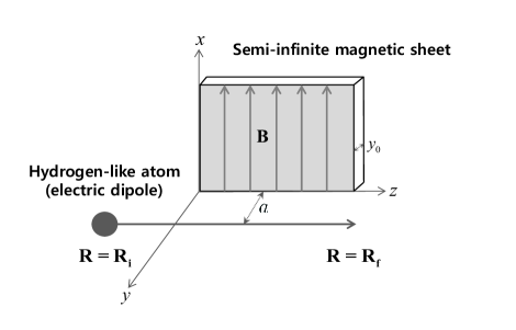
Figure 1: Schematic setup for detection of the geometric phase: A hydrogenlike atom is moving parallel to a distant semi-infinite magnetic sheet. The accumulated phase shift $\phi_{g}$ due to the field interaction can be detected by monitoring the final state of the dipole (see Eq. (21b)).

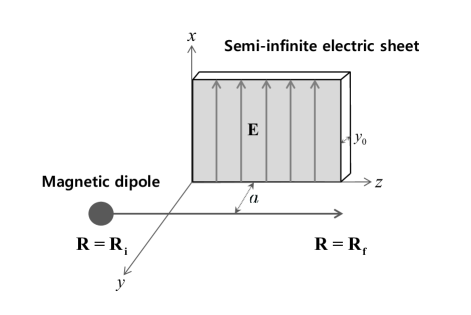
Figure 2: Schematic setup for detection of $\phi_{g}^{m}$, the Maxwell dual of $\phi_{g}$: A particle with spin $1/2$ is moving parallel to a distant semi-infinite sheet of electric field.

References

- Aharonov and Bohm (1959) Y. Aharonov and D. Bohm, Phys. Rev. 115, 485 (1959).
- Peshkin and Tonomura (1989) M. Peshkin and A. Tonomura, in The Aharonov-Bohm Effect (1989), vol. 340.
- He and McKellar (1993) X.-G. He and B. H. McKellar, Phys. Rev. A 47, 3424 (1993).
- Wilkens (1994) M. Wilkens, Phys. Rev. Lett. 72, 5 (1994).
- Spavieri (1998) G. Spavieri, Phys. Rev. Lett. 81, 1533 (1998).
- Wilkens (1998) M. Wilkens, Phys. Rev. Lett. 81, 1534 (1998).
- Kang (2013) K. Kang, arXiv:1308.2093 (2013).
- Kang (2015a) K. Kang, Phys. Rev. A 91, 052116 (2015a).
- Kang (2015b) K. Kang, arXiv:1512.02765 (2015b).
- (10) To be precise, it is necessary to maintain both terms of the right-hand side of Eq. (3) to get a correct classical equation of motion including the source of the external field, even when in the lab frame. However, it does not affect evaluation of a quantum phase. (See discussion in Ref. Kang, 2013).
- Gasiorowicz (2007) S. Gasiorowicz, Quantum physics (John Wiley & Sons, 2007).
- Jackson (1962) J. D. Jackson, Classical electrodynamics (Wiley, 1962).
- Aharonov and Casher (1984) Y. Aharonov and A. Casher, Phys. Rev. Lett. 53, 319 (1984).
- Dowling et al. (1999) J. P. Dowling, C. P. Williams, and J. Franson, Phys. Rev. Lett. 83, 2486 (1999).
- Popescu (2010) S. Popescu, Nat. Phys. 6, 151 (2010).