An Improved Lower Bound for General Position Subset Selection

Abstract

In the General Position Subset Selection (GPSS) problem, the goal is to find the largest possible subset of a set of points such that no three of its members are collinear. If $s_{\textrm{GPSS}}$ is the size of the optimal solution, $\sqrt{s_{\textrm{GPSS}}}$ is the current best guarantee for the size of the solution obtained using a polynomial time algorithm. In this paper we present an algorithm for GPSS to improve this bound based on the number of collinear pairs of points. We experimentally evaluate this and few other GPSS algorithms; the result of these experiments suggests further opportunities for obtaining tighter lower bounds for GPSS.

Keywords: General Position Subset Selection, Collinearity testing, Computational geometry

1 Introduction

A subset of a set of $n$ points in the plain is in general position if no three of its members are on the same line. The NP-complete General Position Subset Selection (GPSS) problem asks for the largest possible such subset. This problem, the fame of which is partly due to the fact that several algorithms in computational geometry assume that their input points are in general position, has received relatively little attention in its general setting. The well-known No-Three-In-Line problem, which is a special case of GPSS, asks for the maximum number of points, no three of which are collinear in an $n\times n$ grid. A lower bound of $(3/2-\epsilon)n$ was proved for this problem [1] and it is conjectured that the best lower bound for large $n$ is $cn$ [2], in which $c$ is $\frac{\pi}{\sqrt{3}}$. No-Three-In-Line has also been extended to three dimensions [3].

Lower bounds for GPSS were proved by Payne and Wood for the case in which the number of collinear points is bounded [4]. More precisely, if no more than $\ell\leq\sqrt{n}$ of input points are collinear, they showed that the size of the largest subset of points in general position is $\Omega(\sqrt{\frac{n}{\ln\ell}})$. More recently Froese et al. proved that GPSS is NP-complete and APX-hard [5]. They also presented several fixed-parameter tractability results for this problem, including a kernel of size $15k^{3}$.

A problem closely related to GPSS is Point Line Cover (PLC). The goal in PLC is to find the minimum number of lines that cover a set of points. This problem has been minutely studied and an approximation algorithm with performance ratio $\log(s_{\textrm{PLC}})$ has been presented for this problem [6], in which $s_{\textrm{PLC}}$ is the size of the optimal solution to PLC. PLC can be used to prove bounds for GPSS [7]: given that at most two points can be selected from each line of a line cover, clearly $s_{\textrm{GPSS}}\leq 2\cdot s_{\textrm{PLC}}$, in which $s_{\textrm{GPSS}}$ is the size of the optimal solution to GPSS. Also, since ${s_{\textrm{GPSS}}\choose 2}$ lines are defined for a set of $s_{\textrm{GPSS}}$ points in general position and since all points outside the optimal solution to GPSS should be on at least one such line (due to its maximality), we have $s_{\textrm{PLC}}\leq{s_{\textrm{GPSS}}}^{2}$.

Cao presented a greedy algorithm for GPSS which works as follows [7]. Let $S$ be an empty set initially. For each point $p$ in the set of input points $P$ in some arbitrary order, add $p$ to $S$, unless it is on a line formed by the points present in $S$. It is easy to see that in $S$ no three points can be collinear. On the other hand, due to its incremental construction, $S$ is maximal and no point in $P\setminus S$ can be added to $S$. This algorithm achieves the best known approximation ratio for GPSS [5]. Since each point in an optimal solution $Q$ outside $S$ cannot be added to $S$, it should be on a line defined by the points in $S$, and since there are ${|S|\choose 2}$ such lines and on each of these lines at most two points of $Q$ can appear, $|Q|\leq|S|+2{|S|\choose 2}$. This algorithm, therefore, finds a subset of size at least $\sqrt{s_{\textrm{GPSS}}}$.

In this paper, we try to improve this bound by reformulating the problem using graphs and finding maximal independent sets in them. Given a set $P$ of $n$ points, the algorithm presented in this paper finds a subset in general position with $\max\{2n^{2}\mathbin{/}(\mathrm{coll}(P)+2n),\sqrt{s_{\textrm{GPSS}}}\}$ points, in which $\mathrm{coll}(P)$ is the total number of collinear pairs in lines with at least three points in $P$ (Theorem 3.3). We experimentally evaluate this and three other GPSS algorithms. Our results show that a modification of the algorithm described in the previous paragraph experimentally obtains larger sets and may be used to identify a better lower bound for GPSS.

The paper is organized as follows: in Section 2, we define the notation used in this paper and in Section 3, we describe our algorithm. We start Section 4 with a discussion about the challenges of generating GPSS test cases and how the test cases used in this paper were obtained. We then report the result of our experiments and finally in Section 5 we conclude this paper.

2 Preliminaries and Notation

Let $P$ be a set of $n$ points in the plane. Three or more points of $P$ are collinear if there is a line that contains all of them. Let $L$ be the set of all maximal collinear subsets of $P$. For each point $p$ in $P$, let $L(p)$ be the subset of $L$ containing all elements of $L$ that contain $p$. Also, let $N(p)$ denote the union of all members of $L(p)$, excluding $p$ itself. We define $\mathrm{coll}(p)$ as the size of $N(p)$, $\mathrm{coll}(Q)$ for a subset $Q$ of $P$ as the sum of $\mathrm{coll}(q)$ for every $q$ in $Q$, and $\overline{\mathrm{coll}}(Q)$ as the average value of $\mathrm{coll}(q)$ for every point $q$ in $Q$.

A subset $Q$ of $P$ is noncollinear if, for every $q$ in $Q$, no point in $L(q)$ is present in $Q$. The collinearity graph $G$ of a finite set $P$ of points is the graph that has a vertex for each point in $P$; in this paper we use the same symbol to represent a point in $P$ and its corresponding vertex in $G$. Two vertices $p$ and $q$ are adjacent in $G$ if and only if $p$ is in $N(q)$. It can be observed that the degree of a vertex $p$ in $G$ equals $\mathrm{coll}(p)$. Figure LABEL:coll demonstrates these definitions in a small example.

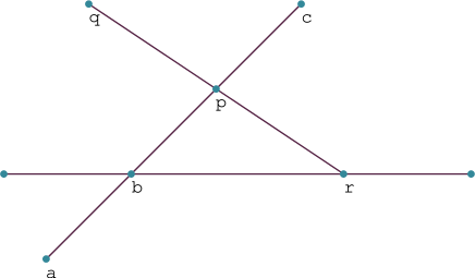
Figure 1: An example configuration of 8 points. Here $L(p)=\{\{p,q,r\},\{a,b,c,p\}\}$, $N(p)=\{a,b,c,q,r\}$, $\mathrm{coll}(p)=5$, and $\mathrm{deg}_{G}(p)=5$.

3 New Lower Bound

Before describing our algorithm, we present two lemmas as follows.

Lemma 3.1.

Any set $P$ of $n$ points contains two disjoint noncollinear subsets $R$ and $T$ such that $|R|+|T|\geq 2n\mathbin{/}(\overline{\mathrm{coll}}(P)+2)$.

Proof.

Let $G=(V,E)$ be the collinearity graph of $P$. The vertex set of $G$ can be decomposed into two subsets $P_{1}$ and $P_{2}$ such that at least half of the edges of $G$ have one endpoint in each of these sets. This can be done as follows. Start with empty $P_{1}$ and $P_{2}$. For every vertex $v$ of $G$ in some order, add it to $P_{1}$ if $v$ has fewer neighbours in $P_{1}$ compared to $P_{2}$, and add it to $P_{2}$, otherwise. Let $P_{1}$ and $P_{2}$ be such a decomposition of $V$ and let $H$ be the graph obtained from $G$ by removing all edges between $P_{1}$ and $P_{2}$. Clearly, since the number of the edges of $H$ is at most half of that of $G$, the average degree of $H$ is also at most half of the average degree of $G$.

Let $S$ be a maximal (that is, non-extensible) independent set in $H$ and let $R=S\cap P_{1}$ and $T=S\cap P_{2}$. Both $R$ and $T$ are independent sets in $H$. Since no edge between the vertices of $P_{1}$ (and hence $R$) is removed in $H$, $R$ is also an independent set in $G$. Symmetrically, $T$ is also an independent set in $G$.

Turan’s lower bound of $n\mathbin{/}(\overline{d}+1)$ for the size of a maximal independent set in a graph with $n$ vertices, in which $\overline{d}$ is the average degree of the graph, can be attained using the greedy algorithm that iteratively selects vertices ordered increasingly by their degrees and removes the selected vertex and its neighbours [8]. Applying Turan’s bound to $H$ yields that $\overline{d}$ is at most half of the average degree of $G$. Hence, we have $\overline{d}\leq\overline{\mathrm{coll}}(P)\mathbin{/}2$, implying that $|S|\geq 2n/(\overline{\mathrm{coll}}(P)+2)$, as required. ∎

The lower bound for the greedy algorithm used in Lemma 3.1 is not the best possible; it is actually a weaker form of the celebrated Caro-Wei lower bound, which has been improved by several authors (see, for instance, [8] and [9]). However, Turan’s bound, which is tight for graphs consisting of disjoint cliques, depends only on the average degree and yields a cleaner bound for the size of noncollinear sets in Lemma 3.1.

Lemma 3.2.

Let $R$ and $T$ be two noncollinear subsets of a set of points $P$. Then, the points in $R\cup T$ are in general position.

Proof.

For each line with at least three points in $P$, each of $R$ and $T$ can include at most one point. Therefore, in their union there are at most two points on each such line in $P$. ∎

We now present our algorithm for finding a subset $S$ of a set of points $P$ in general position (Algorithm 3.1) and prove a lower bound for the size of the set it finds (Theorem 3.3).

1

2

Input : A set $P$ of points in the plane.

Output : A subset $S$ of $P$ in general position.

3 Obtain all maximal subsets $L$ of collinear points in $P$. One way to do this is to move the points to the dual plane; three (or more) points are collinear if their corresponding lines in the dual plane intersect each other at a common point. Regular plane sweeping can identify these intersections. 

4Construct the collinearity graph $G$ from $L$ for the set of input points $P$. 

5Decompose the vertices of $G$ into two sets $P_{1}$ and $P_{2}$, such that there are at least $\mathrm{coll}(P)/2$ edges with one end point in each of these sets, as described in Lemma 3.1. Obtain graph $H$ from $G$ by removing all edges between $P_{1}$ and $P_{2}$. 

6Find a maximal independent set $S$ in $H$ as described in Lemma 3.1. 

Add each point in $P\setminus S$ to $S$, if it and no two points in $S$ are collinear.

Algorithm 3.1 General position subset selection

Theorem 3.3.

Any set $P$ of $n$ points in the plane contains a subset in general position of size at least $\max\{2n^{2}\mathbin{/}(\mathrm{coll}(P)+2n),\sqrt{s_{\textrm{GPSS}}}\}$.

Proof.

We use Algorithm 3.1 to prove this bound. In the step 4 of the algorithm, $S$ has at least $2n\mathbin{/}(\overline{\mathrm{coll}}(P)+2)$ points, as argued in Lemma 3.2. Since $\mathrm{coll}(P)=n\cdot\overline{\mathrm{coll}}(P)$, the minimum size of $S$ can be rewritten as $2n^{2}\mathbin{/}(\mathrm{coll}(P)+2n)$. In step 5, $S$ is made maximal. By the same argument mentioned in the introduction for the greedy GPSS algorithm, it can be shown that after this step the size of $S$ is at least $\sqrt{s_{\textrm{GPSS}}}$. ∎

To evaluate the improvement Theorem 3.3 yields compared to Cao’s algorithm, we experimentally compare them in the next section.

4 Experimental Comparison of GPSS Algorithms

To experimentally evaluate GPSS algorithms, the first challenge is obtaining good test data with a large number of collinear subsets of points. To our knowledge, the available test data are mostly in general position and thus are imperfect for evaluating GPSS algorithms. Therefore, for our purpose it seems necessary to generate point configurations with the desired rate of collinear points. It is, however, very difficult to generate interesting configurations, in which many points appear on each line and each point appears on several lines, forming cycles with different lengths. Indeed, it would be much easier to generate hypergraphs and possibly convert them to point configurations.

A hypergraph can be created from a point configuration by allocating a vertex in the hypergraph to each point and an edge containing the vertices mapped to each maximal set of collinear points. Since lines can intersect in at most one point, each pair of the edges in the resulting hypergraph intersect in at most one vertex; hypergraphs with this property are called linear. The other direction, i.e., obtaining a point configuration from a linear hypergraph is not as trivial though, as the following question states:

Question 4.1.

Given a linear hypergraph, is it possible to map its vertices into points on the two-dimensional plane, such that three of these points are collinear if and only if their corresponding vertices are on the same edge of the hypergraph?

There are hypergraphs for which the answer to the above question is no; the Fano and Pappus configuration without the Pappus line (the line containing the intersection points) are two such examples. It would be interesting to find the exact conditions for which the answer to the above question is yes. In other words, when do linear hypergraphs have a straight-line drawing?

The problem of drawing configurations is closely related to Question 4.1: a $k$-configuration with $n$ vertices, also denoted as an $(n_{k})$-configuration, is a linear hypergraph in which each vertex is in exactly $k$ edges ($k$-regular) and each edge contains exactly $k$ vertices ($k$-uniform) (for a detailed monograph on configurations, the reader may consult [10] or [11]). Being defined more than a century ago, $k$-configurations are one of the oldest combinatorial structures, predating even the definition of hypergraphs. Both the identification of the combinatorial structure of $(n_{k})$ configurations and their geometric realization have been the goal of several mathematicians (Gropp discusses some of the history of $k$-configurations [12] and their realization [13]). Nevertheless, there is still very little known about the structure and the number of geometric and even combinatorial $k$-configurations in general (see for instance [14]).

Even the existence of a fast algorithm for identifying (or finding) geometric $k$-configurations may not help in answering Question 4.1; in a $k$-configuration, some collinear points may not appear in an edge, while the mapping discussed before Question 4.1 requires otherwise.

Question 4.1 also seems to be a generalization of the famous stretchability problem for arrangements of pseudolines. In the stretchability problem, one is given a simple arrangement of pseudolines (any two pseudolines cross exactly once and no three pseudolines meet at one point), and the question is whether the arrangement can be stretched, that is, transformed into an equivalent arrangement of straight lines [15]. For stretchability and similar problems, Schaefer introduced the complexity class ER, for which these problems are complete [16]. In complexity-theoretic hierarchy, this class lies between NP and PSPACE.

The disappointing prospects of answering Question 4.1, even when limited to $k$-configurations, suggest trying other methods for generating interesting GPSS test data.

4.1 Generating Random Hypergraphs

The algorithms discussed in this paper do not directly use the location of the points in the plane. They extract point-line collinearity relations (or equivalently the underlying linear hypergraph) as a first step; therefore, the exact location of the points is not significant in these algorithms. Thus, instead of the locations of the points, these algorithms can take the underlying hypergraph as input.

Although these algorithms expect a linear hypergraph that can be drawn with straight lines, it would still be interesting to evaluate their performance on general linear hypergraphs, especially because of the difficulty of generating configurations with complex point-line collinearity relations. Thus, reminding that the tests considered in this section target a more general problem than GPSS, we generate random linear hypergraphs for testing GPSS algorithms.

Our hypergraph construction is incremental, in contrast to Erdős-Rényi random hypergraphs in which edges are either included or rejected with some probability (see for instance [17]). $H_{d}(n,m)$ is the hypergraph with $n$ vertices and $m$ edges. Initially all edges are empty. The following step is repeated $dn$ times: A vertex $v$ and an edge $e$ are chosen uniformly at random and $v$ is added to $e$, if it does conflict with the linearity of the hypergraph. Given that the above step is repeated $dn$ times, the average degree is at most $d$. The following probabilistic argument obtains a lower bound for the expected average degree of the resulting hypergraph.

We denote with $Prob(R_{i})$ the probability of rejection in the $i$-th step of the algorithm, i.e., when adding vertex $v_{i}$ to edge $e_{i}$. The rejection happens if i) $v_{i}$ already belongs to $e_{i}$, or ii) $v_{i}$ is on an edge $e_{j}$, one of whose vertices $v_{k}$ appears on $e_{i}$ (if $v_{i}$ is added to $e_{j}$, the hypergraph is no longer linear due to the intersections of $e_{i}$ and $e_{j}$). Let $P_{i}(v\in e)$ be the probability of vertex $v$ being added to edge $e$ in one of the first $i$-th steps.

$$Prob(R_{i+1})\leq P_{i}(v_{i}\in e_{i})+\sum_{j=1}^{m}\sum_{k=1}^{n}P_{i}(v_{i}\in e_{i})P_{i}(v_{k}\in e_{j})P_{i}(v_{k}\in e_{i})$$

Given that $P_{i}(v\in e)\leq\frac{i}{nm}$, the probability of rejection can be simplified as follows.

$$Prob(R_{i+1})\leq\frac{i}{nm}+\frac{i^{3}}{nm^{2}}$$

To obtain the expected value of the total number of rejections ($R$), we add up $Prob(R_{i})$ for all rounds of the algorithm (except the first one, which is never rejected):

$$Exp(R)\leq\sum_{i=2}^{dn}Prob(R_{i})\leq\sum_{i=1}^{dn-1}\frac{i}{nm}+\sum_{i=1}^{dn-1}\frac{i^{3}}{nm^{2}}$$

Simplifying this inequality, we obtain:

$$Exp(R)<\frac{3d^{2}n}{4m}$$

Thus the expected average degree ($d_{\textrm{avg}}$) is:

$$Exp(d_{\textrm{avg}})\geq d-\frac{3d^{2}}{4m}$$

4.2 Evaluating GPSS Algorithms

We evaluate the following four GPSS algorithms.

Ind

Algorithm 3.1, which constructs the result by merging two disjoint noncollinear subsets.

Inc [7]

The greedy algorithm described in the Introduction, which constructs a subset of input points by iteratively adding points in some arbitrary order, unless they are collinear with two other points in the set.

Inc-Min

Like Inc except that in each iteration the point with the minimum number of collinear points (among the remaining points) is selected.

Dec

Starts with all points in the set and iteratively removes the points with the most number of collinearity relations with other points in the set.

These algorithm are evaluated on two sets of test cases. The first set is obtained based on the method described in Section 4.1. The second set is generated by placing point on the two-dimensional plane in some pattern, mostly grids. The implementation of the algorithms and the test cases are available at https://github.com/aligrudi/gpss.

Table 1 shows the average ratio of the size of the set returned by any of the algorithms to the largest reported set. The Inc-Min algorithm finds largest sets, outperforming other algorithms by at least three percent on average. Although the performance of Ind is close to Inc-Min, there is an observable gap in their performance.

Table 1: Average ratio of the size of the set returned by each algorithm to the size of the best reported set

Algorithm	Average Ratio to the Best
Ind	96.6
Inc	82.2
Inc-Min	99.4
Dec	87.4

Table 2: The ratio of the number of times each algorithm finds the largest set

Algorithm	Ratio of Best Performance
Ind	41.3
Inc	9.5
Inc-Min	92.1
Dec	20.6

Table 2 shows the ratio of the number of cases in which each algorithm finds the largest set in general position; this again suggests that Inc-Min obtains the largest sets most of the time. These results suggest that it may be possible to obtain a better lower bound for GPSS, based on Inc-Min.

5 Concluding Remarks

GPSS can also be formulated in terms of Hypergraph strong independence. However, it is very surprising that the extensive studies on independence number of hypergraphs are mostly focused on weak independence (see [18] for a summary), in which the independent set can include any but not all of the vertices of each edge.

References

- [1] R. R. Hall, T. H. Jackson, A. Sudbery, and K. Wild. Some advances in the no-three-in-line problem. Journal of Combinatorial Theory Series A, 18(3):336–341, 1975.
- [2] R. K. Guy and P. A. Kelly. The no-three-in-line problem. Canadian Mathematical Bulletin, 11:527–531, 1968.
- [3] A. Por and D. R. Wood. No-three-in-line-in-3d. Algorithmica, 47(4):481–488, 2007.
- [4] M. S. Payne and D. R. Wood. On the general position subset selection problem. SIAM Journal on Discrete Mathematics, 27(4):1727–1733, 2013.
- [5] V. Froese, I. Kanj, A. Nichterlein, and R. Niedermeier. Finding points in general position. In The Canadian Conference on Computational Geometry, pages 7–14, 2016.
- [6] S. Kratsch, G. Philip, and S. Ray. Point line cover: The easy kernel is essentially tight. ACM Transactions on Algorithms, 12(3):40:1–40:16, 2016.
- [7] C. Cao. Study on Two Optimization Problems: Line Cover and Maximum Genus Embedding. MSc Thesis, Texas A&M University, 2012.
- [8] M. M. Halldórsson and J. Radhakrishnan. Greed is good: Approximating independent sets in sparse and bounded-degree graphs. Algorithmica, 18(1):145–163, 1997.
- [9] J. Harant. A lower bound on independence in terms of degrees. Discrete Applied Mathematics, 159(10):966–970, 2011.
- [10] B. Grünbaum. Configurations of Points and Lines. American Methematical Society, 2009.
- [11] T. Pisanski and B. Servatius. Configurations from a Graphical Viewpoint. Springer, 2012.
- [12] H. Gropp. Configurations between geometry and combinatorics. Discrete Applied Mathematics, 138(1–2):79–88, 2004.
- [13] H. Gropp. Configurations and their realization. Discrete Mathematics, 174(1-3):137–151, 1997.
- [14] J. Bokowski and V. Pilaud. On topological and geometric configurations. European Journal of Combinatorics, 50:4–17, 2015.
- [15] N. E. Mnev. The universality theorems on the classification problem of configuration varieties and convex polytopes varieties, pages 527–543. Springer Berlin Heidelberg, 1988.
- [16] M. Schaefer. Complexity of some geometric and topological problems. In Graph Drawing, pages 334–344, 2009.
- [17] A. Dudek, A. Frieze, A. Ruciński, and M. Šileikis. Embedding the erdős–rényi hypergraph into the random regular hypergraph and hamiltonicity. Journal of Combinatorial Theory, Series B, 122:719–740, 2017.
- [18] A. Eustis. Hypergraph Independence Number. PhD Thesis, University of California, San Diego, 2013.