Scene Flow to Action Map: A New Representation for RGB-D based
Action Recognition with Convolutional Neural Networks

Abstract

Scene flow describes the motion of 3D objects in real world and potentially could be the basis of a good feature for 3D action recognition. However, its use for action recognition, especially in the context of convolutional neural networks (ConvNets), has not been previously studied. In this paper, we propose the extraction and use of scene flow for action recognition from RGB-D data. Previous works have considered the depth and RGB modalities as separate channels and extract features for later fusion. We take a different approach and consider the modalities as one entity, thus allowing feature extraction for action recognition at the beginning. Two key questions about the use of scene flow for action recognition are addressed: how to organize the scene flow vectors and how to represent the long term dynamics of videos based on scene flow. In order to calculate the scene flow correctly on the available datasets, we propose an effective self-calibration method to align the RGB and depth data spatially without knowledge of the camera parameters. Based on the scene flow vectors, we propose a new representation, namely, Scene Flow to Action Map (SFAM), that describes several long term spatio-temporal dynamics for action recognition. We adopt a channel transform kernel to transform the scene flow vectors to an optimal color space analogous to RGB. This transformation takes better advantage of the trained ConvNets models over ImageNet. Experimental results indicate that this new representation can surpass the performance of state-of-the-art methods on two large public datasets.

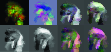
Figure 1: Samples of variants of SFAM for action “Bounce Basketball” from M${}^{\textbf{2}}$I Dataset [21]. For top-left to bottom-right, the images correspond to SFAM-D, SFAM-S, SFAM-RPf, SFAM-RPb, SFAM-AMRPf, SFAM-AMRPb, SFAM-LABRPf, SFAM-LABRPb.

1 Introduction

Recognition of human actions from RGB-D data has generated renewed interest in the computer vision community due to the recent availability of easy-to-use and low-cost depth sensors (e.g. Microsoft Kinect ™sensor). In addition to tristimulus visual data captured by conventional RGB cameras, depth data are provided in RGB-D cameras, thus encoding rich 3D structural information of the entire scene. Previous works [28, 16, 10, 58, 61, 13] showed the effectiveness of fusing the two modalities for 3D action recognition. However, all the previous methods consider the depth and RGB modalities as separate channels from which to extract features and fuse them at a later stage for action recognition. Since the depth and RGB data are captured simultaneously, it will be interesting to extract features considering them jointly as one entity. Optical flow-based methods for 2D action recognition [48, 18, 31, 30, 50] have provided the state-of-the-art results for several years. In contrast to optical flow which provides the projection of the scene motion onto the image plane, scene flow [41, 6, 26, 8, 11, 37, 32] estimates the actual 3D motion field. Thus, we propose the use of scene flow for 3D action recognition. Differently from the optical flow-based late fusion methods on RGB and depth data, scene flow extracts the real 3D motion and also explicitly preserves the spatial structural information contained in RGB and depth modalities.

There are two critical issues that need to be addressed when adopting scene flow for action recognition: how to organize the scene flow vectors and how to effectively exploit the spatio-temporal dynamics. Two kinds of motion representations can be identified: Lagrangian motion [48, 18, 31, 50, 30, 56] and Eulerian motion [2, 25, 60, 51, 52, 1]. Lagrangian motion focuses on individual points and analyses their change in location over time. Such trajectories requires reliable point tracking over long term and is prone to error. Eulerian motion considers a set of locations in the image and analyses the changes at these locations over time, thus avoiding the need for point tracking.

Since scene flow vectors could be noisy and to avoid the difficulty of long term point tracking of Lagrangian motion, we adopted the Eulerian approach in constructing the final representation for action recognition. Furthermore, the scene flow between two consecutive pair of RGB-D frames (two RGB images and two corresponding depth images) is one simple Lagrangian motion with only two frames matching/tracking. This property provides a better representation than is possible with Eulerian motion obtained from raw pixels.

However, it remains unclear as to how video could be effectively represented and fed to deep neural networks for classification. For example, one can conventionally consider a video as a sequence of still images with some form of temporal smoothness, or as a subspace of images or image features, or as the output of a neural network encoder. Which one among these and other possibilities would result in the best representation in the context of action recognition is not well understood. The promising performance of existing temporal encoding works [51, 52, 56, 1] provides a source of motivation. These works encode the spatio-temporal information as dynamic images and enable the use of existing ConvNets models directly without training the whole networks afresh. Thus, we propose to encode the RGB-D video sequences based on scene flow into one motion map, called Scene Flow to Action Map (SFAM), for 3D action recognition. Intuitively and similarly to the three channels of color images, the three elements of a scene flow vector can be considered as three channels. Such consideration allows the scene flow between two consecutive pairs of RGB-D frames to be reorganized as one three-channel Scene Flow Map (SFM), and the RGB-D video sequence can be represented as SFM sequence. In the spirits of Eulerian motion and rank pooling methods [5, 1], we propose to encode SFM sequence into SFAM. Several variants of SFAM are developed. They capture the spatio-temporal information from different perspectives and are complementary to each other for final recognition. However, two issues arise with these hand-crafted SFAMs: 1) direct organization of the scene flow vectors in SFM may sacrifice the relations among the three elements; 2) in order to take advantage of available model trained over ImageNet, the input needs to be analogous to RGB images; that is, the input for the ConvNets need to have similar properties to conventional RGB images as used in trained filters. Based on these two observations, we propose to learn Channel Transform Kernels with rank pooling method and ConvNets, that convert the three channels into suitable three new channels capable of exploiting the relations among the three elements and have similar RGB image features. With this transformation, the dynamic SFAM can describe both the spatial and temporal information of a given video. It can be used as the input to available and already trained ConvNets along with fine-tuning.

The contributions of this paper are summarized as follows:1) The proposed SFAM is the first attempt, to our best knowledge, to extract features from depth and RGB modalities as joint entity through scene flow, in the context of ConvNets; 2) we propose an effective self-calibration method that enables the estimation of scene flow from unregistered captured RGB-D data; 3) several variants of SFAM that encode the spatio-temporal information from different aspects and are complementary to each other for final 3D action recognition are proposed; 4) we introduce Channel Transform Kernels which learn the relations among the three channels of SFM and convert the scene flow vectors to RGB-like images to take advantages of trained ConvNets models and 5) the proposed method achieved state-of-the-art results on two relatively large datasets.

The reminder of this paper is organized as follows. Section 2 describes the related work. Section 3 introduces the SFAM and its variants, and presents the proposed Channel Transform Kernels. Experimental results on two datasets are provided in Section 4. Section 5 concludes the paper and discusses future work.

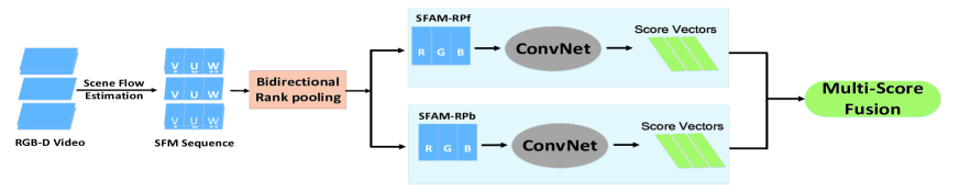
Figure 2: Illustration of Multiply-Score Fusion for SFAM-RP.

2 Related Work

2.1 Feature Extraction from RGB-D Data

Since the first work [20] on 3D action recognition from depth data captured by commodity depth sensors (e.g., Microsoft Kinect ™) in 2010, many methods for action recognition have been proposed based on depth, RGB or skeleton data. These methods either extracted features from one modality: depth [49, 60, 29, 59, 24, 51, 52] or RGB [27, 33] or skeleton [43, 55, 56, 4, 34, 19], or fuse the features extracted separately from them at a later stage [28, 16, 10, 58]. Neither of these methods considered depth and RGB modalities jointly in feature extraction. In contrast, we propose to adopt scene flow for 3D action recognition and extract features jointly from RGB-D data.

2.2 Scene Flow

In general, scene flow is defined as the dense or semi-dense non-rigid motion field of a scene observed at different instants of time [41, 37, 32]. The term “scene flow” was firstly coined by Vedula et al. [41] who proposed to start by computing the Lucas-Kanade optical flow and applied the range flow constraint equation at a later stage. Since this work, several methods [64, 57, 44] have been proposed based on stereo or multiple view camera systems. With the advent of affordable RGB-D cameras, scene flow methods for RGB-D data have also been proposed [41, 8, 37, 32]. However most of the existing methods incur high computational burden, taking from several seconds to a few hours to compute the scene flow per frame. Thus, limiting their usefulness in real applications. Recently, a primal-dual framework for real-time dense RGB-D scene flow [11] has been proposed. A primal-dual algorithm is applied to solve the variational formulation of the scene flow problem. It is an iterative solver performing pixel-wise updates and can be efficiently implemented on GPUs. In this paper, we used this algorithm for scene flow calculation.

2.3 Deep Leaning based Action Recognition

Existing deep learning approaches for action recognition can be generally divided into four categories based on how the video is represented and fed to a deep neural network. The first category views a video either as a set of still images [62] or as a short and smooth transition between similar frames [35], and each color channel of the images is fed to one channel of a ConvNet. Although obviously suboptimal, considering the video as a bag of static frames performs reasonably well. The second category represents a video as a volume and extend ConvNets to a third, temporal dimension [12, 39] replacing 2D filters with 3D equivalents. So far, this approach has produced little benefits, probably due to the lack of annotated training data. The third category treats a video as a sequence of images and feed the sequence to an Recurrent Neural Network (RNN) [3, 4, 42, 34, 22, 23]. An RNN is typically considered as memory cells, which are sensitive to both short as well as long term patterns. It parses the video frames sequentially and encodes the frame-level information in the memory. However, using RNNs did not give an improvement over temporal pooling of convolutional features [62] or even over hand-crafted features. The last category represents a video in one or multiple compact images and adopt available trained ConvNet architectures for fine-tuning [51, 52, 56, 1, 9, 53, 54]. This category has achieved state-of-the-art results in action recognition on many RGB and depth/skeleton datasets. The proposed method in this paper falls into this last category.

3 Scene Flow to Action Map

SFAM encodes the dynamics of RGB-D sequences based on scene flow vectors. To make our description self-contained, in Section 3.1 we briefly present the primal-dual framework for real-time dense RGB-D scene flow computation (hereafter denoted by PD-flow [11]). For scene flow computation, we assume that the depth and RGB data are prealigned. If this is not the case, the videos can be quickly realigned as described in Section 3.2. Then, in Section 3.3 we present several hand-crafted constructions of SFAM and we propose an end-to-end learning method for SFAM through Channel Transform Kernels in Section 3.4.

3.1 PD-flow

The PD-flow estimates the dense 3D motion field of a scene between two instants of time $t$ and $t+1$ using RGB and depth images provided by an RGB-D camera. This motion field $\textbf{M}:(\Omega\in\mathbb{R}^{2})\rightarrow\mathbb{R}^{3}$ defined over the image domain $\Omega$, is described with respect to the camera reference frame and expressed in meters per second. For simplicity, the bijective relationship $\Gamma:\mathbb{R}^{3}\rightarrow\mathbb{R}^{3}$ between M and $\textbf{s}=(\mu,\upsilon,\omega)^{T}$ is given by:

$$\textbf{M}=\Gamma(\textbf{s})=\begin{pmatrix}\frac{Z}{f_{x}}&0&\frac{X}{Z}\\ 0&\frac{Z}{f_{y}}&\frac{Y}{Z}\\ 0&0&1\\ \end{pmatrix}\begin{pmatrix}\mu\\ \upsilon\\ \omega\\ \end{pmatrix},$$ (1)

where $\mu,\upsilon$ represent the optical flow and $\omega$ denotes the range flow; $f_{x},f_{y}$ are the camera focal length values, and $X,Y,Z$ the spatial coordinates of the observed point. Thus, estimating the optical and range flows is equivalent to estimating the 3D motion field but leads to a simplified implementation. In order to compute the motion field a minimization problem over s is formulated where photometric and geometric consistency are imposed as well as a regularity of the solution:

$$\min\limits_{\textbf{s}}\{E_{D}(\textbf{s})+E_{R}(\textbf{s})\}.$$ (2)

In Eq. (2), $E_{D}(\textbf{s})$ is the data term, representing a two-fold restriction for both intensity and depth matching between pairs of frames; $E_{R}(\textbf{s})$ is the regularization term which both smooths the flow field and constrains the solution space.

For data term $E_{D}(\textbf{s})$, the $L_{1}$ norm of photometric consistency $\rho_{I}(\textbf{s},x,y)$ and geometric consistency $\rho_{z}(\textbf{s},x,y)$ is minimized as:

$$E_{D}(\textbf{s})=\int|\rho_{I}(\textbf{s},x,y)|+\varepsilon(x,y)|\rho_{z}(\textbf{s},x,y)|dxdy,$$ (3)

where $\varepsilon(x,y)$ is a positive function that weights geometric consistency against brightness constancy; $\rho_{I}(\textbf{s},x,y)=I_{0}(x,y)-I_{1}(x+\mu,y+\upsilon)$ and $\rho_{z}(\textbf{s},x,y)=\omega-Z_{1}(x+\mu,y+\upsilon)+Z_{0}(x,y)$ with $I_{0},I_{1}$ being the intensity images while $Z_{0},Z_{1}$ the depth images taken at instants $t$ and $t+1$.

The regularization term $E_{R}(\textbf{s})$ is based on the total variation and takes into consideration the geometry of the scene which is formulated as:

$$E_{R}(\textbf{s})=\lambda_{I}\int_{\Omega}|(r_{x}\frac{\partial\mu}{\partial x},r_{y}\frac{\partial\mu}{\partial y})|+|(r_{x}\frac{\partial\upsilon}{\partial x},r_{y}\frac{\partial\upsilon}{\partial y})|dxdy$$

$$+\lambda_{D}\int_{\Omega}|(r_{x}\frac{\partial\omega}{\partial x},r_{y}\frac{\partial\omega}{\partial y})|dxdy,$$ (4)

where $\lambda_{I},\lambda_{D}$ are constant weights and $r_{x}=\frac{1}{\sqrt{\frac{\partial X^{2}}{\partial x}+\frac{\partial Z^{2}}{\partial x}}}$, $r_{y}=\frac{1}{\sqrt{\frac{\partial Y^{2}}{\partial y}+\frac{\partial Z^{2}}{\partial y}}}$.

As the energy function (Eq. (2)) is based on a linearisation of the data term (Eq. (3)) and convex TV regularizer (Eq. (4)), the energy function can be solved using convex solver. An iterative solver can be obtained by deriving the energy function (Eq. (2)) as its primal-dual formulation and implemented in parallel on GPUs. For more implementation details, the keen reader is recommended to read [11].

3.2 Self-Calibration

Scene flow computation requires that the RGB and depth data be spatially aligned and temporally synchronized. The data considered in this paper were captured by Kinect sensors and are temporally synchronized. However, the RGB and depth channels may not be spatially registered if calibration was not performed properly before recording the data. For the RGB-D datasets with spatial misalignment, we propose an effective self-calibration method to perform spatial alignment without knowledge of the cameras parameters. The alignment is based on a pinhole model through which depth maps are transformed into the same view of the RGB video. Let $p_{i}$ be a point in an RGB frame and $p_{i}^{\prime}$ be the corresponding point in the depth map. The 2D homography mapping $H$ satisfying $p_{i}=Hp_{i}^{\prime}$ is a $3\times{}3$ projective transformation for the alignment. Following the method in [7], we chose a set of matching points in an RGB frame and its corresponding depth map. Using four pairs of corresponding points, $H$ is obtained through direct linear transformation. Let $p_{i}^{\prime}=(x_{i}^{\prime},y_{i}^{\prime},1)^{T}$, $h_{j}^{T}$ be the $j_{th}$ row of $H$ and $\textbf{0}=[0,0,0]^{T}$. The vector cross product equation $p_{i}\times{}Hp_{i}^{\prime}=\textbf{0}$ is written as [7]:

$$\left[\begin{array}[]{ccc}\textbf{0}^{T}&-p_{i}^{T}&y_{i}^{\prime}p_{i}^{T}\\ p_{i}^{T}&\textbf{0}^{T}&-x_{i}^{\prime}p_{i}^{T}\end{array}\right]\left(\begin{array}[]{c}h_{1}\\ h_{2}\\ h_{3}\end{array}\right)=\textbf{0},$$ (5)

where the up-to-scale equation is omitted. A better estimation of $H$ is achieved by minimising (for example, using Levenberg-Marquardt algorithm [15]) the following objective function with more matching points: c arg min_^H,^p_i,^p_i’∑_i[d(p_i,^p_i)^2+d(p_i’,^p_i’)]
s.t. ^p_i=^H^p_i’ for ∀i

In Eq. (5), $d(\cdot)$ is the distance function and $\hat{H}$ is the optimal estimation of the homography mapping while $\hat{p_{i}}$ and $\hat{p_{i}}^{\prime}$ are estimated matching points from $\{p_{i},p_{i}^{\prime}\}$. Because the process of selecting matching points may not be reliable, the random sample consensus (RANSAC) algorithm is applied to exclude outliers. By transforming the depth map using the 2D projective transformation $H$, the RGB video and its corresponding depth video are spatially aligned.

3.3 Construction of Hand-crafted SFAM

SFAM encodes a video sample into a single dynamic image to take advantage of the available pre-trained models for standard ConvNets architecture without training millions of parameters afresh. There are several ways to encode the video sequences into dynamic images [2, 25, 60, 51, 52, 1], but how to encode the scene flow vectors into one dynamic image still needs to be explored. As described in Section 3.1, one scene flow vector $\textbf{s}=(\mu,\upsilon,\omega)^{T}$ is obtained by matching/tracking one point in the current frame to another in the reference frame; this is one simple Lagrangian motion. In order to avoid error in tracking Lagrangian motion over long term, we construct SFAM using the Eulerian motion approach and thus, the SFAM inherits the merits of both the Eulerian and Lagrangian motion. As we argued earlier, the three entries ($\mu,\upsilon,\omega$) in the scene flow vector s for each point can be considered as three channels. Hence a scene flow between two pairs of RGB-D images ($I_{0}$, $Z_{0}$ and $I_{1}$, $Z_{1}$) can be reorganized as one three-channel SFM ($X_{\mu}$, $X_{\upsilon}$, $X_{\omega}$), and the RGB-D video sequences can be represented as SFM sequences. Based on the SFM sequences, there are several ways to construct the SFAM.

3.3.1 SFAM-D

Inspired by the construction of Depth Motion Maps (DMM) [60], we accumulate the absolute differences between consecutive SFMs and denote it as SFAM-D. It is written as:

$$\text{SFAM-D}_{i}=\sum\limits_{t=1}^{T-1}|X_{i}^{t+1}-X_{i}^{t}|~{}~{}~{}~{}i\in(\mu,\upsilon,\omega),$$ (6)

where $t$ denotes the map number and $T$ represents the total number of maps (the same for the following sections). This representation characterizes the distribution of the accumulated motion difference energy.

3.3.2 SFAM-S

Similarly to SFAM-D, we construct the SFAM-S (S here denotes the sum) by accumulating the sum between consecutive SFMs. This can be written as:

$$\text{SFAM-S}_{i}=\sum\limits_{t=1}^{T-1}(X_{i}^{t+1}+X_{i}^{t})~{}~{}~{}~{}i\in(\mu,\upsilon,\omega).$$ (7)

This representation mainly captures the large motion of an action after normalization.

3.3.3 SFAM-RP

Inspired by the work reported in [1], we adopt the rank pooling method to encode SFM sequence into one action image. Let $X_{1},...,X_{T}$ denote the SFM sequence where each $X_{t}$ contains three channels ($X_{\mu}$, $X_{\upsilon}$, $X_{\omega}$), and $\varphi(X_{t})\in\mathbb{R}^{d}$ be a representation or feature vector extracted from each individual map, $X_{t}$. Herein, we directly apply rank pooling to the $X$, thus, $\varphi(\cdot)$ equals to identity matrix. Let $V_{t}=\dfrac{1}{t}\sum_{\tau=1}^{t}\varphi(X_{\tau})$ be time average of these features up to time $t$. The ranking function associates with each time $t$ a score $S(t|\textbf{d})=<\textbf{d},V_{t}>$, where $\textbf{d}\in\mathbb{R}^{d}$ is a vector of parameters. The function parameters d are learned so that the scores reflect the order of the maps in the video. In general, more recent frames are associated with larger scores, i.e. $~{}q>t\Rightarrow S(q|\textbf{d})>S(t|\textbf{d})$. Learning d is formulated as a convex optimization problem using RankSVM [36]:

$$\textbf{d}^{*} =\rho(X_{1},...,X_{T};\varphi)=\mathop{\arg\min}_{\textbf{d}}E(\textbf{d}),$$ (8)

$$E(\textbf{d}) =\dfrac{\lambda}{2}\parallel\textbf{d}\parallel^{2}+$$

$$\dfrac{2}{T(T-1)}\times\sum\limits_{q>t}\max\{{0,1-S(q|\textbf{d})+S(t|\textbf{d})}\}.$$

The first term in this objective function is the usual quadratic regular term used in SVMs. The second term is a hinge-loss soft-counting how many pairs $q>t$ are incorrectly ranked by the scoring function. Note in particular that a pair is considered correctly ranked only if scores are separated by at least a unit margin, $i.e.~{}S(q|\textbf{d})>S(t|\textbf{d})+1$.

Optimizing the above equation defines a function $\rho(X_{1},...,X_{T};\varphi)$ that maps a sequence of $T$ SFMs to a single vector $\textbf{d}^{*}$. Since this vector contains enough information to rank all the frames in the SFM sequence, it aggregates information from all of them and can be used as a sequence descriptor. In our work, the rank pooling is applied in a bidirectional manner to convert each SFM sequence into two action maps, SFAM-RPf (forward) and SFAM-RPb (backward). This representation captures the different types of importance associated with frames in one action and assigns more weight to recent frames.

3.3.4 SFAM-AMRP

In previous sections, all the three channels are considered as separate channels in constructing SFAM. However, the specific relationship (independent or otherwise) between them is yet to be ascertained. To study this relationship, we adopt a simple method viz., using amplitude of the scene flow vector s to represent the relations between the three components. Thus, for each triple ($X_{\mu}$, $X_{\upsilon}$, $X_{\omega}$) we obtain a new amplitude map, $X_{am}$. Based on the $X_{am}=\sqrt{X_{\mu}^{2}+X_{\upsilon}^{2}+X_{\omega}^{2}}$, the rank pooling method is applied to encode the scene flow maps into two action maps, SFAM-AMRPf and SFAM-AMRPb. This representation exploits the weights of frames based on the motion magnitude.

3.3.5 SFAM-LABRP

To further investigate the relationship amongst the triple ($X_{\mu}$, $X_{\upsilon}$, $X_{\omega}$), they are transformed nonlinearly into another space, similarly to the manner of transforming RGB color space to Lab space. The Lab space is designed to approximate the human visual system. Based on these transformed maps, the rank pooling method is applied to encode the sequence into two action maps, SFAM-LABRPf and SFAM-LABRPb.

A few examples of the SFAM variants are shown in Figure 1 for action “Bounce Basketball” from M${}^{\textbf{2}}$I Dataset [21]. It can be seen that different variants of SFAM capture and encode SFM sequence into action maps with large visual differences.

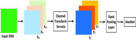
Figure 3: The framework for constructing SFAM with Channel Transform Kernels using ConvNets.

3.4 Constructing SFAM with Channel Transform Kernels (SFAM-CTKRP)

In previous sections, we have presented the concept of SFAM and its several variants. However, it has been empirically observed that none of them can achieve the best results for all the datasets or scenarios. One reason adduced for this is that during the construction of the SFAM, the relationship amongst the triple ($X_{\mu}$, $X_{\upsilon}$, $X_{\omega}$) are hand-crafted. To learn the relationship amongst the elements of the triple ($X_{\mu}$, $X_{\upsilon}$, $X_{\omega}$) from data with ConvNets, we propose a Channel Transform Kernels as follows. Let $Y_{1},Y_{2},Y_{3}$ be the new learned maps from the original triple ($X_{\mu}$, $X_{\upsilon}$, $X_{\omega}$), the relationship between them can be formulated as:

$$Y_{1}=\varphi_{1}(\omega_{1}X_{\mu}+\omega_{2}X_{\upsilon}+\omega_{3}X_{\omega})$$

$$Y_{2}=\varphi_{2}(\omega_{4}X_{\mu}+\omega_{5}X_{\upsilon}+\omega_{6}X_{\omega})$$ (9)

$$Y_{3}=\varphi_{3}(\omega_{7}X_{\mu}+\omega_{8}X_{\upsilon}+\omega_{9}X_{\omega})$$

where $Y$ has the same size with $X$, $\omega$ are scalar values and $\varphi$ denotes the transforms that need to be learned. The learning framework is illustrated in Figure 3. There are different ways to learn these Channel Transform Kernels. For sake of simplicity, in this work we approximated the transforms by three successive convolution layers, where each layer comprises nine convolutional kernels with size $1\times 1$ and followed by ReLU nonlinear transform, as illustrated in Figure 4. Based on RankPool layer [1] for temporal encoding, we can construct the SFAM with the proposed Channel Transform Kernels using ConvNets.

3.5 Multiply-Score Fusion for Classification

After construction of the several variants of SFAM, we propose to adopt one effective late score fusion method, namely, multiply-score fusion method, to improve the final recognition accuracy. Take SFAM-RP for example, as illustrated in Figure 2, two SFAM-RP, one SFAM-RPf and one SFAM-RPb, are generated for one pair of RGB-D videos and they are fed into two different trained ConvNets channels. The score vectors output by the two ConvNets are multiplied element-wisely and the max score in the resultant vector is assigned as the probability of the test sequence. The index of this max score corresponds to the recognized class label. This process can be easily extended into multiple channels.

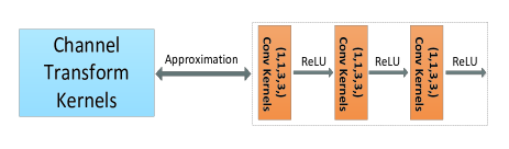
Figure 4: Illustration of approximate computation for Channel Transform Kernels using convolution kernels followed by nonlinear transforms.

4 Experiments

According to the survey of RGB-D datasets [63], we chose two public benchmark datasets, which contain both RGB+depth modalities and have relatively large training samples to evaluate the proposed method. Specifically we chose ChaLearn LAP IsoGD Dataset [46] and M${}^{\textbf{2}}$I Dataset [21]. In the following, we proceed by briefly describing the implementation details and then present the experiments and results.

4.1 Implementation Details

For scene flow computation, we adopted the public codes provided by [11]. For rank pooling, we followed the work reported in [1] where each channel was generated into one channel dynamic map and then merged the three channels into one three-channel map. Differently from [1], we used bidirectional rank pooling. For ChaLearn LAP IsoGD Dataset, in order to minimize the interference of the background, it is assumed that the background in the histogram of depth maps occupies the last peak representing far distances. Specifically, pixels whose depth values are greater than a threshold defined by the last peak of the depth histogram minus a fixed tolerance (0.1 was set in our experiments) are considered as background and removed from the calculation of scene flow by setting their depth values to zero. Through this simple process, most of the background can be removed and has much contribution to the SFAM.

The AlexNet [17] was adopted in this paper. The training procedure of the hand-crafted SFAMs was similar to that described in [17]. The network weights were learned using the mini-batch stochastic gradient descent with the momentum set to 0.9 and weight decay set to 0.0005. All hidden weight layers used the rectification (RELU) activation function. At each iteration, a mini-batch of 256 samples was constructed by sampling 256 shuffled training samples. All the images were resized to 256 $\times$ 256. The learning rate was set to $10^{-3}$ for fine-tuning with pre-trained models on ILSVRC-2012, and then it was decreased according to a fixed schedule, which was kept the same for all training sets. Different datasets underwent different iterations according to their number of training samples. For all experiments, the dropout regularization ratio was set to 0.5 in order to reduce complex co-adaptations of neurons in the nets. The implementation was derived from the publicly available Caffe toolbox [14] based on one NVIDIA Tesla K40 GPU card. Unless otherwise specified, all the networks were initialized with the models trained over ImageNet [17]. For SFAM-CTKRP, we revised the codes of paper [1] based on MatConvNet [40]. The multiply score fusion method is compared with the other two commonly used late score fusion methods, average and maximum score fusion on both datasets. This verifies that the SFAMs are likely to be statistically independent and provide complementary information.

4.2 ChaLearn LAP IsoGD Dataset

The ChaLearn LAP IsoGD Dataset [46] includes 47933 RGB-D depth sequences, each RGB-D video representing one gesture instance. There are 249 gestures performed by 21 different individuals. This dataset does not provide the true depth values in their depth videos. To use this dataset for scene flow calculation, we estimate the depth values using the average minimum and maximum values provided for CGD dataset. The dataset is divided into training, validation and test sets. As the test set is not available for public usage, we report the results on the validation set. For this dataset the training underwent 25K iterations and the learning rate decreased every 10K iterations.

Results. Table 1 shows the results of six variants of SFAM, and compares them with methods in the literature [45, 46, 1, 52]. Among these methods, MFSK combined 3D SMoSIFT [47] with (HOG, HOF and MBH) [48] descriptors. MFSK+DeepID further included Deep hidden IDentity (Deep ID) feature [38]. Thus, these two methods utilized not only hand-crafted features but also deep learning features. Moreover, they extracted features from RGB and depth separately, concatenated them together, and adopted Bag-of-Words (BoW) model as the final video representation. The other methods, WHDMM+SDI [52, 1], extracted features and conducted classification with ConvNets from depth and RGB individually and adopted multiply-score fusion for final recognition.

Compared with these methods, the proposed SFAM outperformed all of them significantly. It is worth noting that all the depth values used in the proposed SFAM were estimated rather than the exact real depth values. Despite the possible estimation errors, our method still achieved promising results. Interestingly, the proposed variants of SFAM are complementary to each other and can improve each other largely by using multiply-score fusion. Even though this dataset is large, on average 144 video clips per class, it is still much smaller compared with 1200 images per class in ImageNet. Thus, directly training from scratch cannot compete with fine-tuning the trained models over ImageNet and this is evident in the results reported in Table 1. By comparing different types of SFAM, we can see that the simple SFAM-S method achieved the best results among all types of hand-designed SFAMs. Due to the relatively large training data, SFAM-CTKRP achieved the best result among all the variants, even though the approximate rank pooling in the work reported in [1] was shown to be worse than rank pooling solved by RankSVM [36]. The reasons for these two phenomenona probably are as follows: under the inaccurate estimation of the depth values, the scene flow computation will be affected and based on this inaccurate scene flow vectors, rank pooling can not achieve its full efficacy. In other words, the rank pooling method is sensitive to noise. Instead, the proposed Channel Transform Kernels cannot only exploit the relations amongst the channels but also decrease the effects of noise after channel transforms.

Method	Accuracy
MFSK [45, 46]	18.65%
MFSK+DeepID [45, 46]	18.23%
SDI [1]	20.83%
WHDMM [52]	25.10%
WHDMM+SDI [52, 1]	25.52%
SFAM-D (training from scratch)	9.23%
SFAM-D	18.86%
SFAM-S (training from scratch)	18.10%
SFAM-S	25.83%
SFAM-RP	23.62%
SFAM-AMRP	18.21%
SFAM-LABRP	23.35%
SFAM-CTKRP	27.48%
Max-Score Fusion All	33.24%
Average-Score Fusion All	34.86%
Multiply-Score Fusion All	36.27%

Table 1: Results and Comparison on the ChaLearn LAP IsoGD Dataset.

4.3 M${}^{\textbf{2}}$I Dataset

Multi-modal & Multi-view & Interactive (M${}^{\textbf{2}}$I) Dataset [21] provides person-person interaction actions and person-object interaction actions. It contains both the front and side views; denoted as Front View (FV) and Side View (SV). It consists of 22 action categories and a total of 22 unique individuals. Each action was performed twice by 20 groups (two persons in a group). In total, M${}^{\textbf{2}}$I dataset contains 1760 samples (22 actions $\times$ 20 groups $\times$ 2 views $\times$ 2 run). For evaluation, all samples were divided with respect to the groups into a training set (8 groups), a validation set (6 groups) and a test set (6 groups). The final action recognition results are obtained with the test set. For this dataset the training underwent 6K iterations and the learning rate decreased every 3K iterations.

Results. We followed the experimental settings as in [21] and compared the results on two scenarios: single task scenario and cross-view scenario. The baseline methods were based on iDT features [48] generated from optical flow and has been shown to be very effective in 2D action recognition. Specifically, for the BoW framework, a set of local spatio-temporal features were extracted, including iDT-Tra, iDT-HOG, iDT-HOF, iDT-MBH, iDT-HOG+HOF, iDT-HOF+MBH and iDT-COM (concatenation of all descriptors); for fisher vector framework, they only used the iDT-COM feature for evaluation. For comparisons, we only show several best results achieved by baseline methods for each scenario. Table 2 shows the comparisons on the M${}^{\textbf{2}}$I Dataset for single task scenario, that is, learning and testing in the same view while Table 3 presents the comparisons for cross-view scenario. Due to the lack of training data, SFAM-CTKRP could not converge steadily and the results varied largely, thus, we did not show its results. For this dataset, SFAM-AMRP achieved the best result for side view while SFAM-LABRP achieved the best result for front view. From Table 2 we can see that for scene flow estimation based on real true depth values, the rank pooling-based method achieved better results than SFAM-D and SFAM-S, which are consistent with the conclusion in [21]. SFAM-AMRP achieved the best results for two cross-view scenarios which can be seen from Table 3. Interestingly, even though our proposed SFAM did not solve any transfer learning problem as in [21] but directly training with the side/front view and testing in the front/side view, it still outperformed the best baseline method significantly, especially in the SV $\rightarrow$ FV setting. This bonus advantage reflects the effectiveness of proposed method.

Method	Accuracy
	SV	FV
iDT-Tra (BoW) [21]	69.8%	65.8%
iDT-COM (BoW) [21]	76.9%	75.3%
iDT-COM (FV) [21]	80.7%	79.5%
iDT-MBH (BoW) [21]	77.2%	79.6%
SFAM-D	71.2%	83.0%
SFAM-S	70.1%	75.0%
SFAM-RP	79.9%	81.8%
SFAM-AMRP	82.2%	78.0%
SFAM-LABRP	72.0%	83.7%
Max-Score Fusion All	87.6%	88.8%
Average-Score Fusion All	88.2%	89.1%
Multiply-Score Fusion All	89.4%	91.2%

Table 2: Comparison on the M${}^{\textbf{2}}$I Dataset for single task scenario (learning and testing in the same view).

Method	Accuracy
	SV $\rightarrow$ FV	FV $\rightarrow$ SV
iDT-Tra [21]	43.3%	39.2%
iDT-COM [21]	70.2%	67.7%
iDT-HOG+MBH [21]	75.8%	71.8%
iDT-HOG+HOF [21]	78.2%	72.1%
SFAM-D	66.7%	65.2%
SFAM-S	68.2%	60.2%
SFAM-RP	71.6%	65.2%
SFAM-AMRP	77.7%	66.7%
SFAM-LABRP	76.9%	65.9%
Max-Score Fusion All	84.7%	73.8%
Average-Score Fusion All	85.3%	75.3%
Multiply-Score Fusion All	87.6%	76.5%

Table 3: Comparison on the M${}^{\textbf{2}}$I Dataset for cross-view scenario.(SV $\rightarrow$ FV: learning in the side view and test in the front view; FV $\rightarrow$ SV: learning in the front view and testing in the side view.)

5 Conclusion and Future Work

We propose a novel method for action recognition based on scene flow. In particular, scene flow vectors are estimated from registered RGB and depth data. A new representation based on scene flow vectors, SFAM, and several variants that capture the spatio-temporal information from different perspectives are proposed for 3D action recognition. In order to exploit the relationships amongst the three channels of scene flow map, we propose to learn the Channel Transform Kernels, end-to-end, with ConvNets from data. Experiments on two benchmark datasets have demonstrated the effectiveness of the proposed method. For the future work, we will improve the temporal encoding method based on scene flow vectors.

References

- [1] H. Bilen, B. Fernando, E. Gavves, A. Vedaldi, and S. Gould. Dynamic image networks for action recognition. In CVPR, 2016.
- [2] A. F. Bobick and J. W. Davis. The recognition of human movement using temporal templates. IEEE Transactions on pattern analysis and machine intelligence, 23(3):257–267, 2001.
- [3] J. Donahue, L. Anne Hendricks, S. Guadarrama, M. Rohrbach, S. Venugopalan, K. Saenko, and T. Darrell. Long-term recurrent convolutional networks for visual recognition and description. In CVPR, pages 2625–2634, 2015.
- [4] Y. Du, W. Wang, and L. Wang. Hierarchical recurrent neural network for skeleton based action recognition. In CVPR, pages 1110–1118, 2015.
- [5] B. Fernando, S. Gavves, O. Mogrovejo, J. Antonio, A. Ghodrati, and T. Tuytelaars. Rank pooling for action recognition. IEEE Transactions on Pattern Analysis and Machine Intelligence, 2016.
- [6] S. Hadfield and R. Bowden. Scene particles: Unregularized particle-based scene flow estimation. IEEE transactions on pattern analysis and machine intelligence, 36(3):564–576, 2014.
- [7] R. Hartley and A. Zisserman. Multiple view geometry in computer vision. Cambridge university press, 2003.
- [8] M. Hornacek, A. Fitzgibbon, and C. Rother. Sphereflow: 6 DoF scene flow from RGB-D pairs. In CVPR, pages 3526–3533, 2014.
- [9] Y. Hou, Z. Li, P. Wang, and W. Li. Skeleton optical spectra based action recognition using convolutional neural networks. IEEE Transactions on Circuits and Systems for Video Technology, 2016.
- [10] J.-F. Hu, W.-S. Zheng, J. Lai, and J. Zhang. Jointly learning heterogeneous features for RGB-D activity recognition. In CVPR, pages 5344–5352, 2015.
- [11] M. Jaimez, M. Souiai, J. Gonzalez-Jimenez, and D. Cremers. A primal-dual framework for real-time dense RGB-D scene flow. In ICRA, pages 98–104, 2015.
- [12] S. Ji, W. Xu, M. Yang, and K. Yu. 3D convolutional neural networks for human action recognition. Pattern Analysis and Machine Intelligence, IEEE Transactions on, 35(1):221–231, 2013.
- [13] C. Jia and Y. Fu. Low-rank tensor subspace learning for rgb-d action recognition. IEEE Transactions on Image Processing, 25(10):4641–4652, 2016.
- [14] Y. Jia, E. Shelhamer, J. Donahue, S. Karayev, J. Long, R. B. Girshick, S. Guadarrama, and T. Darrell. Caffe: Convolutional architecture for fast feature embedding. In Proc. ACM international conference on Multimedia (ACM MM), pages 675–678, 2014.
- [15] C. Kanzow, N. Yamashita, and M. Fukushima. Withdrawn: Levenberg–marquardt methods with strong local convergence properties for solving nonlinear equations with convex constraints. Journal of Computational and Applied Mathematics, 173(2):321–343, 2005.
- [16] Y. Kong and Y. Fu. Bilinear heterogeneous information machine for RGB-D action recognition. In CVPR, pages 1054–1062, 2015.
- [17] A. Krizhevsky, I. Sutskever, and G. E. Hinton. Imagenet classification with deep convolutional neural networks. In Proc. Annual Conference on Neural Information Processing Systems (NIPS), pages 1106–1114, 2012.
- [18] Z. Lan, M. Lin, X. Li, A. G. Hauptmann, and B. Raj. Beyond gaussian pyramid: Multi-skip feature stacking for action recognition. In CVPR, pages 204–212, 2015.
- [19] C. Li, Y. Hou, P. Wang, and W. Li. Joint distance maps based action recognition with convolutional neural network. IEEE Signal Processing Letters, 2017.
- [20] W. Li, Z. Zhang, and Z. Liu. Action recognition based on a bag of 3D points. In CVPRW, pages 9–14, 2010.
- [21] A.-A. Liu, N. Xu, W.-Z. Nie, Y.-T. Su, Y. Wong, and M. Kankanhalli. Benchmarking a multimodal and multiview and interactive dataset for human action recognition. IEEE Transactions on cybernetics, 2016.
- [22] J. Liu, A. Shahroudy, D. Xu, and G. Wang. Spatio-temporal LSTM with trust gates for 3D human action recognition. In Proc. European Conference on Computer Vision, pages 816–833, 2016.
- [23] J. Liu and G. Wang. Global context-aware attention lstm networks for 3d action recognition. In CVPR, 2017.
- [24] C. Lu, J. Jia, and C.-K. Tang. Range-sample depth feature for action recognition. In CVPR, pages 772–779, 2014.
- [25] J. Man and B. Bhanu. Individual recognition using gait energy image. IEEE transactions on pattern analysis and machine intelligence, 28(2):316–322, 2006.
- [26] M. Menze and A. Geiger. Object scene flow for autonomous vehicles. In CVPR, pages 3061–3070, 2015.
- [27] B. Ni, P. Moulin, and S. Yan. Pose adaptive motion feature pooling for human action analysis. International Journal of Computer Vision, 111(2):229–248, 2015.
- [28] S. Nie, Z. Wang, and Q. Ji. A generative restricted boltzmann machine based method for high-dimensional motion data modeling. Computer Vision and Image Understanding, pages 14–22, 2015.
- [29] O. Oreifej and Z. Liu. HON4D: Histogram of oriented 4D normals for activity recognition from depth sequences. In CVPR, pages 716–723, 2013.
- [30] X. Peng, L. Wang, X. Wang, and Y. Qiao. Bag of visual words and fusion methods for action recognition: Comprehensive study and good practice. Computer Vision and Image Understanding, 2016.
- [31] X. Peng, C. Zou, Y. Qiao, and Q. Peng. Action recognition with stacked fisher vectors. In ECCV, pages 581–595, 2014.
- [32] J. Quiroga, T. Brox, F. Devernay, and J. Crowley. Dense semi-rigid scene flow estimation from RGBD images. In ECCV, pages 567–582. 2014.
- [33] H. Rahmani and A. Mian. Learning a non-linear knowledge transfer model for cross-view action recognition. In CVPR, pages 2458–2466, 2015.
- [34] A. Shahroudy, J. Liu, T.-T. Ng, and G. Wang. NTU RGB+ D: A large scale dataset for 3D human activity analysis. In CVPR, 2016.
- [35] K. Simonyan and A. Zisserman. Two-stream convolutional networks for action recognition in videos. In NIPS, pages 568–576, 2014.
- [36] A. J. Smola and B. Schölkopf. A tutorial on support vector regression. Statistics and computing, 14(3):199–222, 2004.
- [37] D. Sun, E. B. Sudderth, and H. Pfister. Layered RGBD scene flow estimation. In CVPR, pages 548–556, 2015.
- [38] Y. Sun, X. Wang, and X. Tang. Deep learning face representation from predicting 10,000 classes. In CVPR, 2014.
- [39] D. Tran, L. Bourdev, R. Fergus, L. Torresani, and M. Paluri. Learning spatiotemporal features with 3D convolutional networks. In ICCV, pages 4489–4497, 2015.
- [40] A. Vedaldi and K. Lenc. Matconvnet – convolutional neural networks for matlab. In Proceeding of the ACM Int. Conf. on Multimedia, 2015.
- [41] S. Vedula, P. Rander, R. Collins, and T. Kanade. Three-dimensional scene flow. Pattern Analysis and Machine Intelligence, IEEE Transactions on, 27(3):475–480, 2005.
- [42] V. Veeriah, N. Zhuang, and G.-J. Qi. Differential recurrent neural networks for action recognition. In ICCV, pages 4041–4049, 2015.
- [43] R. Vemulapalli, F. Arrate, and R. Chellappa. Human action recognition by representing 3D skeletons as points in a lie group. In CVPR, pages 588–595, 2014.
- [44] C. Vogel, K. Schindler, and S. Roth. Piecewise rigid scene flow. In ICCV, pages 1377–1384, 2013.
- [45] J. Wan, G. Guo, and S. Z. Li. Explore efficient local features from RGB-D data for one-shot learning gesture recognition. IEEE Transactions on Pattern Analysis and Machine Intelligence, 38(8):1626–1639, Aug 2016.
- [46] J. Wan, S. Z. Li, Y. Zhao, S. Zhou, I. Guyon, and S. Escalera. Chalearn looking at people RGB-D isolated and continuous datasets for gesture recognition. In Proc. IEEE Computer Society Conference on Computer Vision and Pattern Recognition Workshops (CVPRW), pages 1–9, 2016.
- [47] J. Wan, Q. Ruan, W. Li, G. An, and R. Zhao. 3d smosift: three-dimensional sparse motion scale invariant feature transform for activity recognition from rgb-d videos. Journal of Electronic Imaging, 23(2), 2014.
- [48] H. Wang and C. Schmid. Action recognition with improved trajectories. In ICCV, pages 3551–3558, 2013.
- [49] J. Wang, Z. Liu, Y. Wu, and J. Yuan. Mining actionlet ensemble for action recognition with depth cameras. In CVPR, pages 1290–1297, 2012.
- [50] L. Wang, Y. Qiao, and X. Tang. Action recognition with trajectory-pooled deep-convolutional descriptors. In CVPR, pages 4305–4314, 2015.
- [51] P. Wang, W. Li, Z. Gao, C. Tang, J. Zhang, and P. O. Ogunbona. Convnets-based action recognition from depth maps through virtual cameras and pseudocoloring. In ACM MM, pages 1119–1122, 2015.
- [52] P. Wang, W. Li, Z. Gao, J. Zhang, C. Tang, and P. Ogunbona. Action recognition from depth maps using deep convolutional neural networks. Human-Machine Systems, IEEE Transactions on, 46(4):498–509, 2016.
- [53] P. Wang, W. Li, S. Liu, Z. Gao, C. Tang, and P. Ogunbona. Large-scale isolated gesture recognition using convolutional neural networks. In Proceedings of ICPRW, 2016.
- [54] P. Wang, W. Li, S. Liu, Y. Zhang, Z. Gao, and P. Ogunbona. Large-scale continuous gesture recognition using convolutional neural networks. In Proceedings of ICPRW, 2016.
- [55] P. Wang, W. Li, P. Ogunbona, Z. Gao, and H. Zhang. Mining mid-level features for action recognition based on effective skeleton representation. In DICTA, 2014.
- [56] P. Wang, Z. Li, Y. Hou, and W. Li. Action recognition based on joint trajectory maps using convolutional neural networks. In ACM MM, pages 102–106, 2016.
- [57] A. Wedel, T. Brox, T. Vaudrey, C. Rabe, U. Franke, and D. Cremers. Stereoscopic scene flow computation for 3D motion understanding. International Journal of Computer Vision, 95(1):29–51, 2011.
- [58] C. Wu, J. Zhang, S. Savarese, and A. Saxena. Watch-n-patch: Unsupervised understanding of actions and relations. In CVPR, pages 4362–4370, 2015.
- [59] X. Yang and Y. Tian. Super normal vector for activity recognition using depth sequences. In CVPR, pages 804–811, 2014.
- [60] X. Yang, C. Zhang, and Y. Tian. Recognizing actions using depth motion maps-based histograms of oriented gradients. In ACM MM, pages 1057–1060, 2012.
- [61] M. Yu, L. Liu, and L. Shao. Structure-preserving binary representations for rgb-d action recognition. IEEE transactions on pattern analysis and machine intelligence, 38(8):1651–1664, 2016.
- [62] J. Yue-Hei Ng, M. Hausknecht, S. Vijayanarasimhan, O. Vinyals, R. Monga, and G. Toderici. Beyond short snippets: Deep networks for video classification. In CVPR, pages 4694–4702, 2015.
- [63] J. Zhang, W. Li, P. O. Ogunbona, P. Wang, and C. Tang. RGB-D-based action recognition datasets: A survey. Pattern Recognition, 60:86–105, 2016.
- [64] Y. Zhang and C. Kambhamettu. On 3d scene flow and structure estimation. In CVPR, pages 778–785, 2001.