An Optimization Framework with Flexible Inexact Inner Iterations
for Nonconvex and Nonsmooth Programming

Abstract

In recent years, numerous vision and learning tasks have been (re)formulated as nonconvex and nonsmooth programmings (NNPs). Although some algorithms have been proposed for particular problems, designing fast and flexible optimization schemes with theoretical guarantee is a challenging task for general NNPs. It has been investigated that performing inexact inner iterations often benefit to special applications case by case, but their convergence behaviors are still unclear. Motivated by these practical experiences, this paper designs a novel algorithmic framework, named inexact proximal alternating direction method (IPAD) for solving general NNPs. We demonstrate that any numerical algorithms can be incorporated into IPAD for solving subproblems and the convergence of the resulting hybrid schemes can be consistently guaranteed by a series of simple error conditions. Beyond the guarantee in theory, numerical experiments on both synthesized and real-world data further demonstrate the superiority and flexibility of our IPAD framework for practical use.

1 Introduction

Nonconvex and nonsmooth programmings (NNPs) have received wide attentions in recent years [27, 22, 33, 37, 5]. Many problems in vision and learning societies, such as sparse coding and dictionary learning [5], matrix factorization [22], image restoration [37], and image classification [40] can be (re)formulated as specific NNPs. In this work, we consider a general NNP in following formulation:

$$\min_{\mathbf{X}:=(\mathbf{x}_{1},\ldots,\mathbf{x}_{K})}\Psi(\mathbf{X}):=\sum\limits_{i=1}^{K}f_{i}(\mathbf{x}_{i})+H(\mathbf{X}),$$ (1)

where $\mathbf{x}_{i}$s are vectors or matrices throughout the paper.

This general NNP covers a variety of techniques in image processing and machine learning. For example, principal component analysis with sparse constraints, like lasso constraint [26] and elastic-net regularization [40] can be written in problem (1). In non-negative matrix factorization problem [22], it is common to adopt $H$ as a $\ell_{2}$ distance on describing the ability of restoration and restrict $f_{i}$s to be non-negative on each component. Sparse dictionary learning (SDL) can also be formulated in problem (1). Many literatures [18, 27, 5] have posted the superiority on restricting dictionaries with normalized bases while at the same time constraining sparsity for codes with various nonconvex and nonsmooth sparse penalties.

In the past few years, there have been literatures [2, 8, 33, 34, 7] in optimization and numerical analysis on designing converged algorithms in view of the general NNP (1). These algorithms have been applied to various problems, such as non-negative matrix factorization [8], SDL with $\ell_{0}$ penalty [5] and non-negative Tucker decomposition [34]; at the same time, abundant experimental analyses have demonstrated the efficiency and convergence properties of these algorithms. However, in pursuit of convergence, most of the existing algorithms are designed with fixed iteration schemes; those inflexible schemes are tightly constrained and fail to take the model structures of specific problems into consideration.

While on the other hand, specific solvers designed for practical use are far more flexible than the converged algorithms proposed for the general problem (1). Those specific solvers always take advantages of the problem structures and then employ effective numerical methods to solve specific sub-problems. Moreover, we have noticed from previous work [10, 30, 19, 11, 25] that solving sub-problems with inner iterations is a frequently used strategy in numerous efficient solvers. Though few of the inexact solvers are designed with rigid theoretical support and analyses, their efficiencies and convergence properties have been verified from experiments under certain conditions.

1.1 Contributions

Motivated from various inexact solvers, we in this paper propose an unified and flexible algorithm framework named inexact proximal alternating direction method (IPAD). Our IPAD is designed for solving the general NNP problem (1), at the same time, keeping the flexibility when dealing with specific problems. Different from existing solvers in practice, IPAD theoretically give rigid conditions on parameters and stopping criteria to ensure the convergence, thus is more rigid and robust for practical use. The theoretical support provided in this paper can be regarded as a guidance for designing inexact algorithms for solving specific problems in a concise framework. As far as we know, we are the first to incorporate various numerical methods into a general algorithm framework and at the same time give rigorous convergence analyses for NNPs. In summary, our contributions are three folds:

1. Different from most existing numerical algorithms for NNPs, which always fix their updating schemes during iterations, we provide a novel perspective to incorporate different optimization strategies into a unified and flexible proximal optimization framework for (1).

2. Even with inexact subproblems and flexible inner iteration schemes, we prove that the convergence property of the resulting hybrid optimization framework can still be guaranteed. Indeed, our theoretical results are the best we can ask for, unless further assumptions are made on the general NNPs in (1).

3. As an application example, we show implementations of applying IPAD with different inner algorithms to solve the widely concerned $\ell_{0}$ regularized SDL model. Numerical evaluations and abundant experimental comparisons demonstrate promising experimental results of the proposed algorithms, which verify the flexibility and efficiency of our optimization framework.

2 Related Work

2.1 Existing Optimization Strategies for NNPs

In past several years, accompanied with the rising popularity of investigating sparsity and low-rankness (naturally with nonconvex and nonsmooth properties) for vision and learning tasks [22, 37, 32, 1, 23, 39], developing numerical solvers for different types of NNP models have attracted considerable research interests from computer vision, machine learning and optimization societies.

As a typical nonconvex and nonsmooth measurement, $\ell_{0}$ norm has been widely applied for image processing problems [37, 32, 1]; and various methods have been designed for solving its optimization. In [37], the authors propose a proximal method for finding desirable solution to $\ell_{0}$TV problem, but they only prove a weak convergence result under mild conditions. The rank function [23, 39] has also been well studied: the work in [23] optimizes a low-rank minimization by an iteratively reweighted algorithm. However, they can only prove that any limit point is a stationary point, which cannot guarantee the correct convergence of the iterations. Another typical problem, non-negative matrix factorization is a powerful technique for various applications; algorithms like ANLS [22] have been specially designed for solving this specific problem.

On the other hand, some algorithms with rigid theoretical analyses have been proposed for solving the general NNP problem (1) [2, 8, 31]. The authors in [2] propose an algorithm named GIST for solving a special class of NNP (1) and apply it to logistic regression problem. A proximal alternating linearized method is proposed in [8], however, it is time-consuming for solving special problems. Xu et al. in [31] propose a MM method for the general NNP, but their algorithm is too complicated to be implemented in practice. The authors in [2] provide their convergence result by assuming subproblems are exactly solved, however, this condition is unattainable in most situations.

In summary, most optimization schemes for specific NNPs are efficient in practice, however, their convergence guarantees are relatively weak. While, algorithms designed for the general NNP are well-converged, but they always have strict conditions and are inefficient in practice.

2.2 Inexact Inner Iterations in Application Fields

We have observed that in some application fields, relatively good performances are often obtained by “improper” numerical algorithms. In previous literatures [41, 36, 25], the “improper” iteration skills have been frequently used in solving sparse coding, blind kernel estimation, and medical imaging problems in practice.

One of those inexact schemes is employing numerical methods as inner iteration methods for solving special subproblems. For instance, the authors in [41] employ half-quadratic splitting and Lagrangian dual method as the inner iteration schemes for estimating clear images in blind deconvolution problem. While in a text image deblurring paper [25], the authors update variables though alternating direction method, meanwhile, applying half-quadratic splitting for solving subproblems. Although these inexact solvers are effective in practice, they are totally designed in freestyle and are uncontrolled in the performances.

Another kind of inexact schemes is adopting neural networks for approximating exact solutions during iterations. For example, time-unfolded recurrent neural networks can be used to produce the best possible approximations for sparse coding problem [18, 28]. On the other hand, fusing various neural networks in ADMM framework [13, 36] has great performances for approximately optimizing problems for image restoration and compressed sensing. The efficiencies of these inexact solvers and their convergence performances have been verified from experiments, however, few of them are designed with rigid theoretical support.

3 The Proposed Optimization Framework

To simplify subsequent derivations, we propose an IPAD and analyze its properties for problem (1) with $2$ variables:

$$\min\limits_{\mathbf{z}:=(\mathbf{x},\mathbf{y})}\Psi(\mathbf{z}):=f(\mathbf{x})+g(\mathbf{y})+H(\mathbf{x},\mathbf{y}).$$ (2)

Though the whole properties are analyzed for problem (2), it is straightforward to extend them to the general one. Then we give assumptions on the objective function:

(1) $f$ and $g$ are proper, lower semi-continuous functions;

(2) $H$ is a $C^{1}$ function and its gradient is Lipschitz continuous on a bounded set;

(3) $\Psi$ is a coercive, Kurdyka-Łojasiewicz (KŁ) function.

Remark 1

It should be mentioned that the most frequently used $\ell_{2}$-norm $H(\mathbf{x},\mathbf{y})$ is a KŁ function which also satisfies the second assumption. On the other hand, regularizers like $\ell_{0}$ penalty, $\ell_{p}$ norm, SCAD [16], MCP [38] and indicator functions are all KŁ functions and at the same time satisfy the first assumption. Since the finite sums of KŁ functions are also KŁ functions [8], thus not a few models in image processing and machine learning satisfy these assumptions.

3.1 Inexact Proximal Reformulation

For solving problem (2), it is natural and common to apply a proximal alternating direction method (PAD) [35, 11] for alternatively updating variables in a cyclic order:

$$\mathbf{x}^{t}_{\ast} =\arg\min\limits_{\mathbf{x}}f(\mathbf{x})+H(\mathbf{x},\mathbf{y}^{t-1})+\frac{\eta_{1}^{t-1}}{2}\|\mathbf{x}-\mathbf{x}^{t-1}\|^{2},$$ (3)

$$\mathbf{y}^{t}_{\ast} =\arg\min\limits_{\mathbf{y}}g(\mathbf{y})+H(\mathbf{x}^{t},\mathbf{y})+\frac{\eta_{2}^{t-1}}{2}\|\mathbf{y}-\mathbf{y}^{t-1}\|^{2},$$

where $\eta_{1}^{t-1}$ and $\eta_{2}^{t-1}$ are proximal parameters added on the subproblems respectively; the notations $\mathbf{x}^{t}_{\ast}$ and $\mathbf{y}^{t}_{\ast}$ are used to represent exact solutions of the subproblems in Eq. (3). It should be pointed out that adding proximal terms on subproblems is a common skill to improve the stability of algorithms on solving nonconvex problems [2].

As claimed before, in most cases, it is either impossible or extremely hard for calculating exact solutions of subproblems. Thus not a few work employ inner iteration schemes to compute approximations to the exact solutions, which means, the inexact solutions $\mathbf{x}^{t}$ and $\mathbf{y}^{t}$ calculated by inner methods are approximations to $\mathbf{x}^{t}_{\ast}$ and $\mathbf{y}^{t}_{\ast}$:

$$\mathbf{x}^{t}\approx\mathbf{x}^{t}_{\ast},\quad\quad\mathbf{y}^{t}\approx\mathbf{y}^{t}_{\ast}.$$ (4)

We can see from the above that our IPAD is in a general framework: it alternatively updates variables by approximately solving the subproblems of PAD. While on the other hand, it does not restrict specific formulas for solving the subproblems, hence IPAD has quite flexible inner iteration schemes that can fuse efficient numerical methods into.

Algorithm 1 Inexact Proximal Alternating Direction

1:  Setting parameters: $C_{x}$, $C_{y}$, $\{\eta_{1}^{t}\}_{t\in\mathbb{N}}$, $\{\eta_{2}^{t}\}_{t\in\mathbb{N}}$.

2:  Initializing variables: $\mathbf{x}^{0}$, $\mathbf{y}^{0}$.

3:  while not converged do

4:     $\mathbf{x}^{t}=\psi(\mathbf{x};\mathbf{x}^{t-1},\mathbf{y}^{t-1},f,H,\eta_{1}^{t},C_{x})$. (i.e., Perform Alg. 2 for $\mathbf{x}$ subproblem)

5:     $\mathbf{y}^{t}=\psi(\mathbf{y};\mathbf{y}^{t-1},\mathbf{x}^{t},g,H,\eta_{2}^{t},C_{y})$. (i.e., Perform Alg. 2 for $\mathbf{y}$ subproblem)

6:  end while

Algorithm 2 $\mathbf{u}^{t}=\psi(\mathbf{u};\mathbf{u}^{t-1},\mathbf{v},h,H,\eta,C_{u})$.

1:  With parameters $C_{x}$, $C_{y}$, $\{\eta_{1}^{t}\}_{t\in\mathbb{N}}$, $\{\eta_{2}^{t}\}_{t\in\mathbb{N}}$ in Alg. 1.

2:  Denote $\mathcal{A}$ as inner iteration schemes for optimizing $h(\mathbf{u})+H(\mathbf{u},\mathbf{v})+\frac{\eta}{2}\|\mathbf{u}-\mathbf{u}^{t-1}\|^{2}$.

3:  Let $\mathbf{u}^{t,0}=\mathbf{u}^{t-1}$.

4:  while $\|\mathbf{e}_{u}^{t,i}\|>C_{u}\|\mathbf{u}^{t,i}-\mathbf{u}^{t-1}\|$ do

5:     $\mathbf{u}^{t,i}=\mathcal{A}(\mathbf{u}^{t,i-1})$.

6:     In theory, use Eq. (5) to analyze convergence.

7:     In practice, use Eq. (13) for judging criterion.

8:  end while

9:  $\mathbf{u}^{t}=\widetilde{\mathbf{u}}^{t,i}$.

3.2 Flexible Inner Iteration Schemes

Our IPAD framework is highly flexible since it allows fusing any efficient algorithms, to compute inexact solutions for specific subproblems. This flexibility is especially welcomed in practice: since the constraints added on variables are always quite different from one another, efficient algorithms for solving specific subproblems should be carefully chosen. For example, when facing the SDL problem with $\ell_{1}$ regularization [15, 24], both subproblems are convex. Then various numerical methods designed under convex case like homotopy method [14], FISTA [6] and ADMM [9] can be applied to solving these subproblems.

On the other hand, although many previously used inexact solvers can be presented under our IPAD framework [21, 30, 11], almost all the inner iteration schemes are experimentally designed. For example, a 2-step inner loop is supposed to be “good-enough” in [30]; the authors of [21] stop the inner iterations at fixed steps to achieve acceptable solutions. Different from the previous work, we in the following Criterion 1 provide theoretical conditions for stopping the inner iterations.

Since calculating the inexact solutions brings errors $\mathbf{e}_{x}^{t}$ and $\mathbf{e}_{y}^{t}$ in the first-order optimality conditions:

$$\mathbf{e}_{x}^{t} =\mathbf{g}_{x}^{t}+\nabla_{\mathbf{x}}H(\mathbf{x}^{t},\mathbf{y}^{t-1})+\eta_{1}^{t-1}(\mathbf{x}^{t}-\mathbf{x}^{t-1}),$$ (5)

$$\mathbf{e}_{y}^{t} =\mathbf{g}_{y}^{t}+\nabla_{\mathbf{y}}H(\mathbf{x}^{t},\mathbf{y}^{t})+\eta_{2}^{t-1}(\mathbf{y}^{t}-\mathbf{y}^{t-1}),$$

with $\mathbf{g}_{x}^{t}\in\partial f(\mathbf{x}^{t})$ and $\mathbf{g}_{y}^{t}\in\partial g(\mathbf{y}^{t})$, we in the following Criterion 1 show that these errors should be bounded to a certain extent at every iteration.

Criterion 1

The errors $\mathbf{e}_{x}^{t}$ and $\mathbf{e}_{y}^{t}$ in Eq. (5) must satisfy

$$\|\mathbf{e}_{x}^{t}\|\leq C_{x}\|\mathbf{x}^{t}-\mathbf{x}^{t-1}\|,\ \ \|\mathbf{e}_{y}^{t}\|\leq C_{y}\|\mathbf{y}^{t}-\mathbf{y}^{t-1}\|,$$ (6)

where parameters $C_{x}$ and $C_{y}$ are two positive integers defined before the iteration starts.

With the stopping criteria (6) for inner iteration schemes, we summarize the whole algorithm in Alg. 1. However, this inexact framework is still on conceptual progress: the stopping criteria can not be directly calculated from (6) and an implementation should be put forward for carrying IPAD for practical use. Before providing a practical implementation in Sec. 3.4, we first analyze the convergence properties of IPAD with the help of the well-designed Criterion 1.

3.3 Convergence Analyses

In this section, we provide the theoretical support for IPAD method. The strategic point on analyzing the convergence properties of IPAD is regarding $\mathbf{x}^{t+1}$ and $\mathbf{y}^{t+1}$ as the exact solutions on solving the following subproblems:

$$\min\limits_{\mathbf{x}}f(\mathbf{x})+H(\mathbf{x},\mathbf{y}^{t})+\frac{\eta_{1}^{t}}{2}\|\mathbf{x}-\mathbf{x}^{t}\|^{2}-(\mathbf{e}_{x}^{t+1})^{\top}\mathbf{x},$$ (7)

$$\min\limits_{\mathbf{y}}g(\mathbf{y})+H(\mathbf{x}^{t+1},\mathbf{y})+\frac{\eta_{2}^{t}}{2}\|\mathbf{y}-\mathbf{y}^{t}\|^{2}-(\mathbf{e}_{y}^{t+1})^{\top}\mathbf{y}.$$

This equivalent conversion is rigid since the first-order optimality conditions of (7) are exactly the same with Eq. (5). However, it should be emphasized that $\mathbf{x}^{t+1}$ and $\mathbf{y}^{t+1}$ are not computed by directly minimizing (7); this equivalent conversion is nothing but assisting in theoretical analyses.

Before proposing the main theorem, we give the requirements on $\{\eta_{1}^{t}\}_{t\in\mathbb{N}}$ and $\{\eta_{2}^{t}\}_{t\in\mathbb{N}}$.

Assumption 1

Parameters $\{\eta_{1}^{t}\}_{t\in\mathbb{N}}$ and $\{\eta_{2}^{t}\}_{t\in\mathbb{N}}$ satisfy

$$\eta_{1}^{t}>2C_{x},\quad\eta_{2}^{t}>2C_{y},\quad{\rm for\ all\ t\in\mathbb{N}},$$ (8)

to ensure the whole IPAD algorithm converges.

Then with the help of Assumption 1, we can obtain the main theorem in Theorem 1: our proposed IPAD has the best convergence property, that is, the global convergence property for general NNP: our IPAD generates a Cauchy sequence that converges to a critical point of the problem.

Theorem 1

Under the Assumption 1 and suppose the sequence $\{(\mathbf{x}^{t},\mathbf{y}^{t})\}_{t\in\mathbb{N}}$ generated by IPAD is bounded. Then $\{(\mathbf{x}^{t},\mathbf{y}^{t})\}_{t\in\mathbb{N}}$ is a Cauchy sequence that converges to a critical point $(\mathbf{x}^{\ast},\mathbf{y}^{\ast})$ of $\Psi$.

For proving this main convergence theorem, the two assertions in the following key lemma are the cornerstones. From the two assertions, obviously, the objective function $\Psi$ is sufficiently descent (Eq. (9) in Lemma 1) during iterations, which together with the second assertion ensures that there is a subsequence of $\{\mathbf{z}^{t}\}_{t\in\mathbb{N}}$ that converges to a critical point of the problem. By further combining the KŁ property, we have the global convergence property for our proposed IPAD method as claimed in Theorem 1.

Lemma 1

Suppose that the sequence $\{(\mathbf{x}^{t},\mathbf{y}^{t})\}_{t\in\mathbb{N}}$ generated by IPAD is bounded. Then the following two assertions hold under the Assumption 1:

$$\small\Psi(\mathbf{z}^{t})-\Psi(\mathbf{z}^{t+1})\geq a(\|\mathbf{x}^{t+1}-\mathbf{x}^{t}\|^{2}+\|\mathbf{y}^{t+1}-\mathbf{y}^{t}\|^{2}),$$ (9)

$$\small dist(0,\partial\Psi(\mathbf{z}^{t}))\leq b(\|\mathbf{x}^{t}-\mathbf{x}^{t-1}\|+\|\mathbf{y}^{t}-\mathbf{y}^{t-1}\|),$$ (10)

where constants $a=\min_{t\in\mathbb{N}}\{\frac{\eta_{1}^{t}}{4}-\frac{(C_{x})^{2}}{\eta_{1}^{t}},\frac{\eta_{2}^{t}}{4}-\frac{(C_{y})^{2}}{\eta_{2}^{t}}\}$ and $b=\max_{t\in\mathbb{N}}\{\eta_{1}^{t-1}+C_{x},M+\eta_{2}^{t-1}+C_{y}\}$ with Lipschitz constant $M$ of $\nabla H$ on bounded sets.

For the convergence rate, our IPAD method shares the same result with PALM [8] when the desingularising function $\phi(s)=\frac{C}{\theta}s^{\theta}:[0,\mu)\to\mathbb{R}_{+}$ of $\Psi$ is satisfied with positive constant $C$ and $\theta\in[0,1).$ Specifically, IPAD converges in a finite number of steps when $\theta$ equals to 1. For $\theta\in[0,\frac{1}{2})$ and $\theta\in(\frac{1}{2},1)$, IPAD converges with a sublinear rate and a linear rate respectively. Though the convergence rate of IPAD is the same with PALM in theory (the convergence rate is not affected by the algorithm but the objective function $\Psi$ of NNP [17]), the experimental results in Section 4 verify the efficiency of our algorithm.

Remark 2

It is natural to extend IPAD to solving the general multi-block NNP (1). Furthermore, all the convergence analyses conducted on problem (2) can be straightforwardly extended to the multi-block case. Since not a few problems can be (re)formulated as the general formulation (1), thus our IPAD method can be applied for solving a wider range of problems in applications.

We can see from the above contents that, arbitrarily incorporating inner numerical methods into IPAD still ensure the global convergence property of the whole algorithm as long as the stopping criteria (6) and the parameter conditions (8) are satisfied. From this perspective, IPAD is not a single algorithm, but a general and flexible algorithm framework with rigid convergence properties. In addition, through blending other numerical methods into our IPAD framework, some previous inexact methods applied to applications [24, 21, 11] can also be proved to achieve the global convergence property.

3.4 Implementable Error Bound

Though we have given criteria of inexactness in the Criterion 1, there appears another problem: the errors $\mathbf{e}_{x}^{t}$ and $\mathbf{e}_{y}^{t}$ can not be directly calculated. Since $\mathbf{g}_{x}^{t}$ and $\mathbf{g}_{y}^{t}$ in Eq. (5) are unattainable in practice, $\mathbf{e}_{x}^{t}$ and $\mathbf{e}_{y}^{t}$ can not be directly calculated by the equalities in Eq. (5). Thus the aforementioned IPAD algorithm, i.e., Alg. 1 is only in the conceptual progress; the criteria (6) are not implementable in practice.

Instead, we in this section provide a truly implementation for carrying IPAD for practical use. After calculating the inexact solutions $\mathbf{x}^{t}$ and $\mathbf{y}^{t}$ of Eq. (4) by some numerical methods, we first compute two intermediate variables $\widetilde{\mathbf{x}}^{t}$ and $\widetilde{\mathbf{y}}^{t}$ as the solutions of specific proximal mappings

$$\widetilde{\mathbf{x}}^{t}=\mathrm{prox}^{1}_{f}(\mathbf{v}_{x}^{t}),\ \ \ \ \widetilde{\mathbf{y}}^{t}=\mathrm{prox}^{1}_{g}(\mathbf{v}_{y}^{t}),$$ (11)

where variables $\mathbf{v}_{x}^{t}$ and $\mathbf{v}_{y}^{t}$ are computed as follows:

$$\mathbf{v}_{x}^{t} =\mathbf{x}^{t}-\nabla_{\mathbf{x}}H(\mathbf{x}^{t},\mathbf{y}^{t-1})-\eta_{1}^{t-1}(\mathbf{x}^{t}-\mathbf{x}^{t-1}),$$ (12)

$$\mathbf{v}_{y}^{t} =\mathbf{y}^{t}-\nabla_{\mathbf{y}}H(\mathbf{x}^{t},\mathbf{y}^{t})-\eta_{2}^{t-1}(\mathbf{y}^{t}-\mathbf{y}^{t-1}).$$

After getting the intermediate variables $\widetilde{\mathbf{x}}^{t}$ and $\widetilde{\mathbf{y}}^{t}$ from $\mathbf{x}^{t}$ and $\mathbf{y}^{t}$, the errors $\mathbf{e}_{x}^{t}$ and $\mathbf{e}_{y}^{t}$ are calculated by:

$$\mathbf{e}_{x}^{t} =(1-\eta_{1}^{t-1})(\widetilde{\mathbf{x}}^{t}-\mathbf{x}^{t})+\nabla_{\mathbf{x}}H(\mathbf{x}^{t},\mathbf{y}^{t-1})-\nabla_{\mathbf{x}}H(\widetilde{\mathbf{x}}^{t},\mathbf{y}^{t-1}),$$ (13)

$$\mathbf{e}_{y}^{t} =(1-\eta_{2}^{t-1})(\widetilde{\mathbf{y}}^{t}-\mathbf{y}^{t})+\nabla_{\mathbf{y}}H(\mathbf{x}^{t},\mathbf{y}^{t})-\nabla_{\mathbf{y}}H(\mathbf{x}^{t},\widetilde{\mathbf{y}}^{t}).$$

We give a proposition as follows to show that these two errors are exactly the implementable versions of Eq. (5). In order to make discussions smoother, we provide the proof of Proposition 1 at the end of this paper in Appendix A.

Proposition 1

The errors, $\mathbf{e}_{x}^{t}$ and $\mathbf{e}_{y}^{t}$ calculated though the Eq. (13) are equivalent to the ones in Eq. (5).

Thus, the errors in (13) are used for checking whether the stopping criteria (6) are satisfied; once the criteria are satisfied, we re-assign $\widetilde{\mathbf{x}}^{t}$ to $\mathbf{x}^{t}$ and $\widetilde{\mathbf{y}}^{t}$ to $\mathbf{y}^{t}$. Then $\widetilde{\mathbf{x}}^{t}$ and $\widetilde{\mathbf{y}}^{t}$ become the final solutions of their corresponding subproblems at $t$-th step. For clarity, we give the detailed inexact process of inner iteration schemes in Alg. 2.

  (a) $\|\mathbf{W}^{t+1}-\mathbf{W}^{t}\|/\|\mathbf{W}^{t}\|$

  (b) $\|\mathbf{D}^{t+1}-\mathbf{D}^{t}\|/\|\mathbf{D}^{t}\|$

  (c) $\|\Psi^{t+1}-\Psi^{t}\|/\|\Psi^{t}\|$

  (d) Inner Iteration

  (e) $\|\mathbf{W}^{t+1}-\mathbf{W}^{t}\|/\|\mathbf{W}^{t}\|$

  (f) $\|\mathbf{D}^{t+1}-\mathbf{D}^{t}\|/\|\mathbf{D}^{t}\|$

  (g) $\|\Psi^{t+1}-\Psi^{t}\|/\|\Psi^{t}\|$

  (h) Inner Iteration

  (i) $\|\mathbf{W}^{t+1}-\mathbf{W}^{t}\|/\|\mathbf{W}^{t}\|$

  (j) $\|\mathbf{D}^{t+1}-\mathbf{D}^{t}\|/\|\mathbf{D}^{t}\|$

  (k) $\|\Psi^{t+1}-\Psi^{t}\|/\|\Psi^{t}\|$

  (l) Inner Iteration

Figure 1: The convergence properties of using PALM [8], INV [5], IPAD-PITH (PITH for short in the figures), IPAD-ADMM (ADMM for short) and IPAD-P2A (P2A for short) for SDL problem with $\ell_{0}$ penalty on synthetic data. The convergence results in the first row belongs to $n=64$; the second row belongs to $n=144$ and the last row belongs to $n=256$.

4 Experimental Results

Though our IPAD algorithm framework can be directly applied to numerous problems in computer vision and machine learning [40, 21, 27, 11], we in this paper just consider to utilize the widely concerned $\ell_{0}$-regularized SDL model [5] as an example to verify the flexibility and efficiency of our IPAD framework. All the compared algorithms are implemented by Matlab R2013b and tested on a PC with 8 GB of RAM and Intel Core i5-4200M CPU.

4.1 SDL with $\ell_{0}$ Penalty

The SDL problem with $\ell_{0}$ penalty is formulated as:

$$\min_{\mathbf{D},\mathbf{W}}\frac{1}{2}\|\mathbf{I}-\mathbf{D}\mathbf{W}^{\top}\|^{2}+\lambda\|\mathbf{W}\|_{0}+\mathcal{X}_{\mathcal{W}}(\mathbf{W})+\mathcal{X}_{\mathcal{D}}(\mathbf{D}),$$ (14)

where $\|\cdot\|_{0}$ denotes the $\ell_{0}$ penalty that counts the number of non-zero elements of $\mathbf{W}$. Here the indicator function $\mathcal{X}$ acts on the set

$$\mathcal{D}=\{\mathbf{D}=\{\mathbf{d}_{i}\}_{i=1}^{m}\subset\mathbb{R}^{n\times m}:\|\mathbf{d}_{i}\|=1,\forall i\}.$$

As for another set $\mathcal{W}$, we make it empty for synthetic data but define it as

$$\mathcal{W}=\{\mathbf{W}=\{\mathbf{w}_{i}\}_{i=1}^{m}\subset\mathbb{R}^{p\times m}:\|\mathbf{w}_{i}\|_{\infty}\leq U_{b},\forall i\},$$

for real-world data to enhance the stability of the model [5]. Moreover, we denote $\mathcal{S}(\mathbf{W})=\lambda\|\mathbf{W}\|_{0}+\mathcal{X}_{\mathcal{W}}(\mathbf{W})$ to simplify the deduction.

It is observed that problem (14) is a special case of problem (2). Thus, we can apply IPAD for inexactly solving the following subproblems since it is extremely hard to get exact solutions of the subproblems.

$$\small\min_{\mathbf{W}}\mathcal{S}(\mathbf{W})+\frac{1}{2}\|\mathbf{I}-\mathbf{D}^{t}\mathbf{W}^{\top}\|^{2}+\frac{\eta_{1}^{t}}{2}\|\mathbf{W}-\mathbf{W}^{t}\|^{2},$$ (15)

$$\small\min_{\mathbf{D}}\mathcal{X}_{\mathcal{D}}(\mathbf{D})+\frac{1}{2}\|\mathbf{I}-\mathbf{D}(\mathbf{W}^{t+1})^{\top}\|^{2}+\frac{\eta_{2}^{t}}{2}\|\mathbf{D}-\mathbf{D}^{t}\|^{2}.$$ (16)

Moreover, PALM can also be applied to solve (14), but it requires computing Lipschitz constants at every iteration.

Notice that solving the nonconvex subproblem (15) is not a trivial task. Here we apply a proximal iterative hard-thresholding (PITH) algorithm [3, 20] to solve this subproblem. On the other hand, we apply ADMM [9] for solving subproblem (16).

4.2 Synthetic Data

We generate synthetic data with different sizes to help analyze the property of IPAD (see Table 1). All the algorithms for the synthetic data stop when satisfying:

$$\footnotesize\max\left\{\frac{\|\mathbf{D}^{t+1}-\mathbf{D}^{t}\|}{\|\mathbf{D}^{t}\|},\ \frac{\|\mathbf{W}^{t+1}-\mathbf{W}^{t}\|}{\|\mathbf{W}^{t}\|},\ \frac{\|\Psi^{t+1}-\Psi^{t}\|}{\|\Psi^{t}\|}\right\}<1e^{-4},$$ (17)

where $\Psi^{t}$ is the objective value at step $t$.

Data	$n=64,m=600,p=4000$					$n=144,m=900,p=10000$				$n=256,m=1600,p=16000$
Alg.	PALM	INV	PITH	ADMM	P2A	PALM	INV	ADMM	P2A	PALM	INV	ADMM	P2A
Out-iter	104	23	51	22	14	56	33	22	15	31	38	18	12
Time (s)	52.82	7.81	253.56	8.72	8.31	96.08	45.93	35.58	38.94	319.97	253.17	150.25	158.42

Table 1: The number of outer iterations and the iteration time (s) of PALM [8], INV [5], our IPAD-PITH (PITH for short in this table), our IPAD-ADMM (ADMM for short) and our IPAD-P2A (P2A for short) for synthetic data. The results are the averages of multiple tests.

4.2.1 Efficiency of Inexact Strategy

To show the respective effects of using inexact strategies on different subproblems, we propose IPAD-PITH which obtains $\mathbf{W}^{t+1}$ by PITH but keeps $\mathbf{D}$-subproblem the same as PALM. We also design IPAD-ADMM that computes $\mathbf{D}^{t+1}$ by ADMM but remains $\mathbf{W}$-subproblem the same as PALM.

Image / $\sigma$ / $\lambda$	PALM [8]			mPALM [4]			INV [5]			IPAD-ADMM
“Peppers512” / $30$ / $5500$	PSNR	Iter	Time	PSNR	Iter	Time	PSNR	Iter	Time	PSNR	Iter	Time
	28.64	4	4.11	30.11	10	325.53	30.14	61	48.63	30.21	25	23.29
“Lena512” / $25$ / $4500$	PSNR	Iter	Time	PSNR	Iter	Time	PSNR	Iter	Time	PSNR	Iter	Time
	28.85	4	3.98	31.04	14	459.10	31.11	62	50.20	31.13	31	37.78
“Barbara512” / $20$ / $3500$	PSNR	Iter	Time	PSNR	Iter	Time	PSNR	Iter	Time	PSNR	Iter	Time
	28.73	4	4.13	30.06	11	399.19	30.09	58	45.09	30.22	18	16.54
“Hill512” / $15$ / $2500$	PSNR	Iter	Time	PSNR	Iter	Time	PSNR	Iter	Time	PSNR	Iter	Time
	29.84	4	4.03	31.20	26	85.34	31.31	84	69.73	31.32	19	17.81

Table 2: The PSNR scores of the recovered images, number of outer iterations and the whole iteration time (s) of PALM [8], mPALM [4], INV [5] and our IPAD-ADMM for real-world data.

Method	$\sigma=30$	$\sigma=25$	$\sigma=20$	$\sigma=15$
KSVD [15]	PSNR / Time	PSNR / Time	PSNR / Time	PSNR / Time
	29.21 / 184.88	30.09 / 235.22	31.14 / 318.06	32.49 / 481.48
IPAD-ADMM	PSNR / Time	PSNR / Time	PSNR / Time	PSNR / Time
	28.98 / 20.04	29.85 / 26.75	30.89 / 22.72	32.28 / 22.65

Table 3: Quantitative denoising results of KSVD [15] and IPAD-ADMM on 7 widely-used example images.

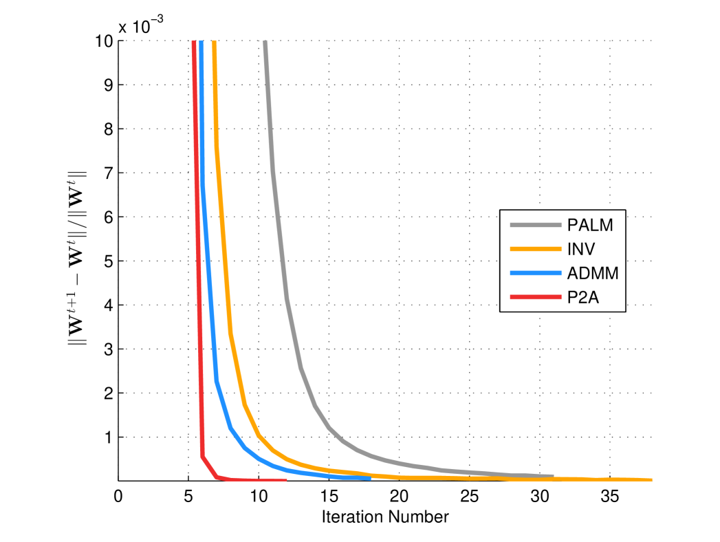
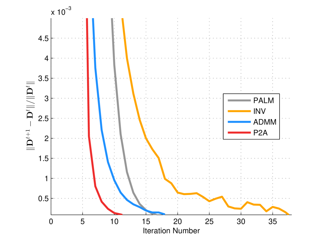
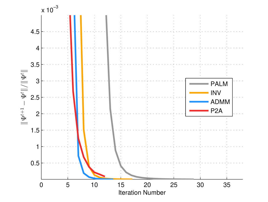
The comparisons in Table 1 among PALM, IPAD-PITH and IPAD-ADMM show that inexact strategies help reduce the iteration steps: both the IPAD-PITH and IPAD-ADMM converges with less iterations than PALM. However, the performances of IPAD-PITH and IPAD-ADMM are quite different in inner iterations. We can see from Figure 1(d) that IPAD-ADMM uses few inner steps during iterations. However, IPAD-PITH reaches the maximum inner steps (set as 20) at almost every iteration. This from one side shows that ADMM is suitable for solving (16) but PITH is less efficient for solving (14). On the other side it is caused by the problems themselves: (16) has unique solution but problem (15) is a challenging NP hard problem and only sub-optimal solution can be found in polynomial time. Since PITH converges with unexpected time, thus we only test it on the data with relatively low dimension ($n=64$).

We also apply inexact strategies to both subproblems of $\mathbf{D}$ and $\mathbf{W}$. Since PITH is time-consuming for solving (15), thus we reduce the maximum inner step to 2 for PITH. We name this algorithm as IPAD-P2A. Then we can see from the Figure 1 and Table 1 that IPAD-P2A uses less iteration steps and sometimes converges faster to an optimal solution.

Remark 3

Though Theorem 1 is proved for applying the inexact strategy to both subproblems, the two hybrid forms of IPAD, i.e. IPAD-PITH and IPAD-ADMM, are also converged. Furthermore, a hybrid IPAD optionally combines PALM, PAM and IPAD can be proved to have global convergence property for solving problem (2)

Remark 4

It can be observed that IPAD-P2A can not be seen as a special case of the hybrid IPAD since it contains one inexact strategy for $\mathbf{D}$ and two-steps prox-linear iterations for $\mathbf{W}$. But fortunately, the experimental results verify the convergence of IPAD-P2A and we can also prove the convergence from theoretical analyses.

By comparing the algorithms, all the inexact strategies of our IPAD method perform better than PALM and are verified to be practicable, converged and efficient. However, a less efficient numerical method for solving subproblem indeed reduce the efficiency of the whole algorithm. Therefore, we suggest carefully choosing effective numerical methods for solving subproblems.

4.2.2 Other Comparisons

At last, we compare INV that solves $\mathbf{W}^{t+1}$ in the same way as PALM but treats $\mathbf{D}^{t+1}$ as the solution of a linear system first and then project the solution on set $\mathcal{D}$. Though this strategy seems to be efficient in practice [5], it lacks theoretical guarantee. Firstly, $\mathbf{D}^{t+1}$ calculated by INV is not an exact solution of (16). Secondly, it is computed without measuring the inexactness. So applying INV sometimes creates oscillations during iterations (Figure 1 (f)) and the performances of INV are unstable especially in real-world applications (see the experimental results in Section 4.3). Thus we do not recommend using it in practice.

(a) “Hill512”, $\sigma=15$

(b) “Child512”, $\sigma=30$

Figure 2: Comparing the convergence performances with various algorithms on two images.

(a) “Couple512”, $\sigma=20$

(b) “Lena512”, $\sigma=25$

Figure 3: Inner iterations of IPAD-ADMM on two examples.

4.3 Real-world Data

We apply IPAD to real-world data on image denoising problem [15, 12] and compare PALM [8], mPALM [4], INV [5] with our IPAD-ADMM for solving this real-world application. All the algorithms for comparison terminate when reaching $\|\mathbf{D}^{t+1}-\mathbf{D}^{t}\|/\|\mathbf{D}^{t}\|<1e^{-2}$ and are demonstrated on 7 widely-used images. The patches in each image, of size $8\times 8$, are regularly sampled in an overlapping manner. The noisy images are obtained by adding Gaussian randomly noises with level $\sigma=15,20,25,30$.

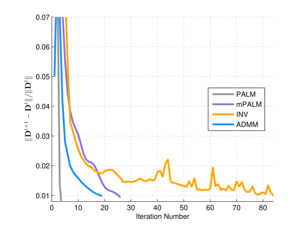
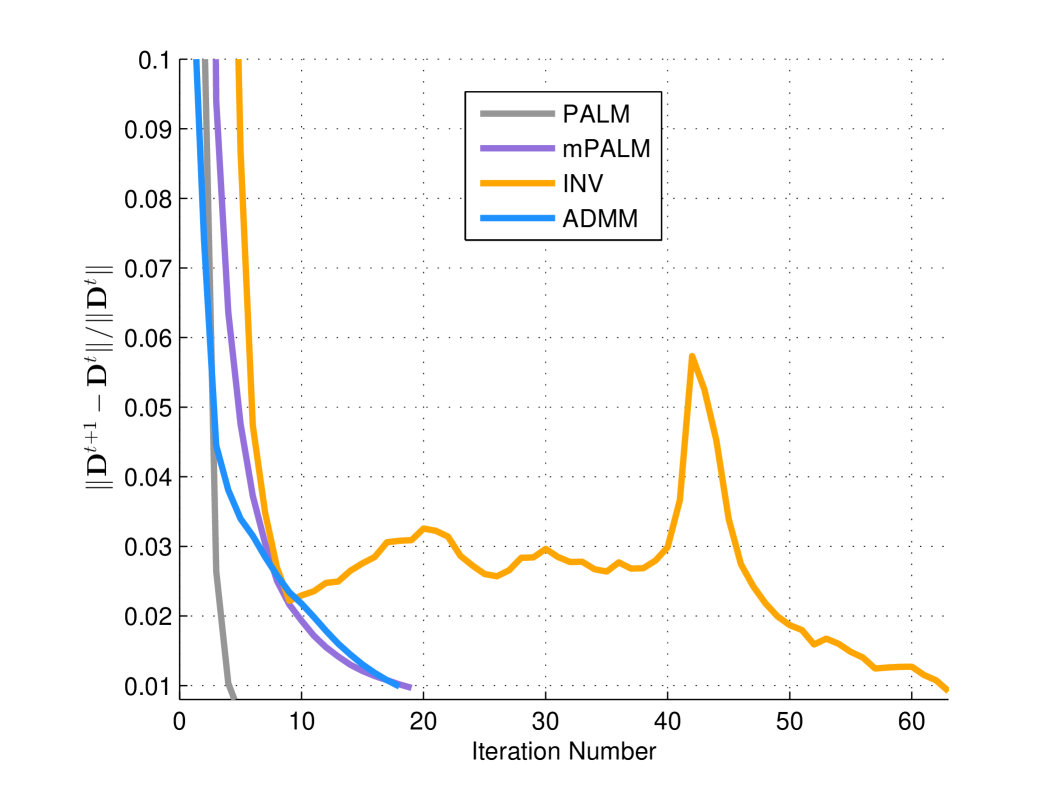
As shown in Table 2, PALM seems to converge quickly but get bad recovered results. However, the truth is: the large upper bound $\|(\mathbf{D}^{t+1})^{\top}\mathbf{D}^{t+1}\|_{2}$ of the Lipschitz constant emphasizes the function of the proximal term. So it causes tiny differences between $\mathbf{D}^{t+1}$ and $\mathbf{D}^{t}$. Thus, PALM does not converge when reaching the stopping criterion; on the contrary, it converges quite slow. For the failure of using PALM, we adopt the strategy used in [4], which regards the problem (14) as a multi-block problem: solving $\{\mathbf{d}_{i}\}_{i=1}^{m}$ separately by PALM. We name their algorithm mPALM and show the results in Table 2. This time, mPALM converges to an acceptable result when reaching the stopping criterion.

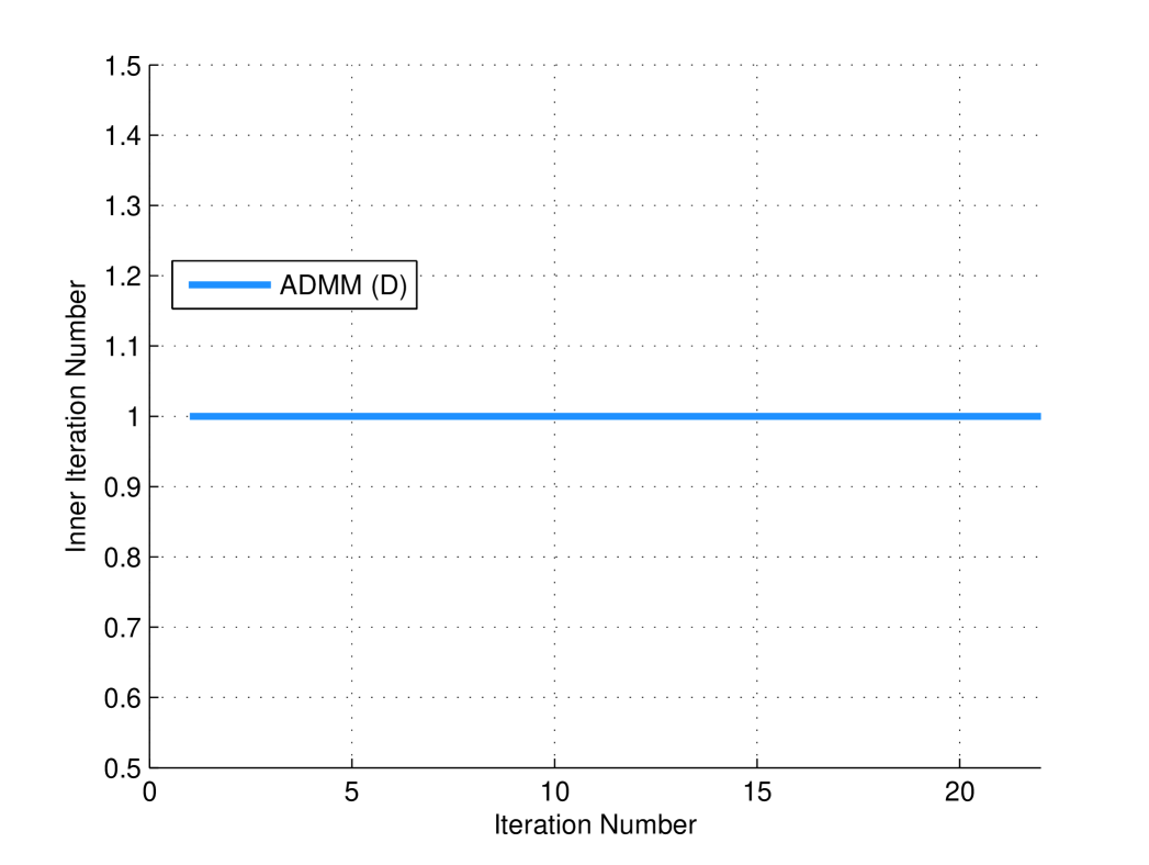
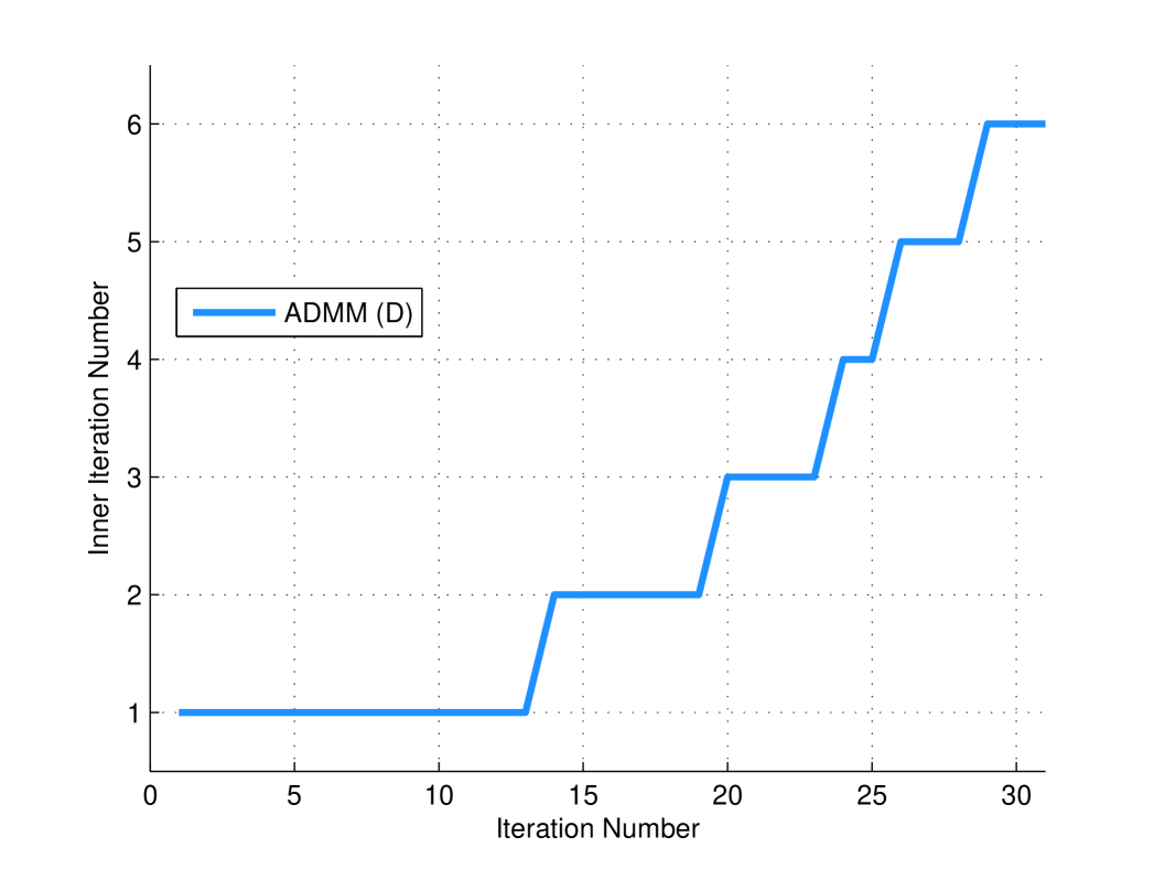
We in Fig. 2 present comparison results on convergence performances: the vibration of INV [5] causes more iterations than IPAD-ADMM. We also select two examples in Fig. 3 to present the inner iteration numbers of our inexact algorithm. It can be seen from the figure that the inner iteration behaviors may be in totally different style; it depends on the input data and algorithm parameters. In addition, we also some visual comparisons in Fig. 4 and 4 to show that our IPAD-ADMM performs more stable and efficient for the real-world applications.

Finally, we give comparisons between the state-of-the-art KSVD technique [15] and our proposed IPAD-ADMM in Table 3. First we want to point it out that KSVD is designed for solving a quasi-$\ell_{0}$ (not the exact $\ell_{0}$ penalty) problem with the usage of OMP [29]. We can see that though our PSNR values are slightly less than KSVD, we use less than a tenth of the time of KSVD. Thus, our IPAD is a fast algorithm with flexible inner iterations for solving the problem SDL with $\ell_{0}$ penalty in practice.

(a) mPALM [4]

(b) INV [5]

(c) IPAD-ADMM

Figure 4: The dictionaries learned by mPALM [4], INV [5] and our IPAD-ADMM on “Barbara512” with $\sigma=20$.

(a) Noisy image

(b) Recovered image

Figure 5: Illustrating image denoising performance on an example image. (a) noisy image with $\sigma=30$, (b) image recovered by IPAD-ADMM.

5 Conclusions

This paper provided a fast optimization framework to solve the challenging nonconvex and nonsmooth programmings (NNPs) in vision and learning societies. Different from most existing solvers, which always fix their updating schemes during iterations, we showed that under some mild conditions, any numerical algorithms can be incorporated into our general algorithmic framework and the convergence of the hybrid iterations can always be guaranteed. We conjectured that our theoretical results are the best we can ask for unless further assumptions are made on the general NNPs in (1). Numerical evaluations on both synthetic data and real images demonstrated promising experimental results of the proposed algorithms.

6 Appendix A: proof of Proposition 1

• From the Alg. 2, at the $t$-th iteration, suppose that an inner iteration scheme is conducted by $K$ time, and denote its current iterative solution as $\mathbf{x}^{t,K}$. Then from the calculations in Eq. (11), we can deduce the following equalities.

  $$\widetilde{\mathbf{x}}^{t,K}= \mathrm{prox}^{1}_{f}(\mathbf{x}^{t,K}-\nabla_{\mathbf{x}}H(\mathbf{x}^{t,K},\mathbf{y}^{t-1})-\eta_{1}^{t-1}(\mathbf{x}^{t,K}-\mathbf{x}^{t-1}))$$ (18)

  $$= \mathrm{prox}^{1}_{f}(\widetilde{\mathbf{x}}^{t,K}-\nabla_{\mathbf{x}}H(\widetilde{\mathbf{x}}^{t,K},\mathbf{y}^{t-1})-\eta_{1}^{t-1}(\widetilde{\mathbf{x}}^{t,K}-\mathbf{x}^{t-1})$$

  $$+ (1-\eta_{1}^{t-1})(\widetilde{\mathbf{x}}^{t,K}-\mathbf{x}^{t,K})$$

  $$+ \nabla_{\mathbf{x}}H(\mathbf{x}^{t,K},\mathbf{y}^{t-1})-\nabla_{\mathbf{x}}H(\widetilde{\mathbf{x}}^{t,K},\mathbf{y}^{t-1})).$$

  Once the error $\mathbf{e}_{x}^{t,K}$ satisfies the inexact condition Crit 1, then $\widetilde{\mathbf{x}}^{t,K}$ will be regarded as the solution of the $t$-th iteration. That is, by substituting the notation $\widetilde{\mathbf{x}}^{t,K}$ with $\mathbf{x}^{t}$ in Eq. (18), thus we get

  $$\mathbf{x}^{t}=\mathrm{prox}^{1}_{f}(\mathbf{x}^{t}-\nabla_{\mathbf{x}}H(\mathbf{x}^{t},\mathbf{y}^{t-1})-\eta_{1}^{t-1}(\mathbf{x}^{t}-\mathbf{x}^{t-1})+\mathbf{e}_{x}^{t}).$$

  The above deductions can be similarly extended to the case of $\mathbf{y}^{t}$. Together with Eq. (12), we have

  $$\mathbf{x}^{t}=\mathrm{prox}^{1}_{f}(\mathbf{v}_{x}^{t}+\mathbf{e}_{x}^{t}),\ \ \mathbf{y}^{t}=\mathrm{prox}^{1}_{g}(\mathbf{v}_{y}^{t}+\mathbf{e}_{y}^{t}).$$ (19)

  From the definition of $\mathrm{prox}$ mapping, Eq. (19) is equal to

  $$\mathbf{e}_{x}^{t} =\mathbf{g}_{x}^{t}+\nabla_{\mathbf{x}}H(\mathbf{x}^{t},\mathbf{y}^{t-1})+\eta_{1}^{t-1}(\mathbf{x}^{t}-\mathbf{x}^{t-1}),$$ (20)

  $$\mathbf{e}_{y}^{t} =\mathbf{g}_{y}^{t}+\nabla_{\mathbf{y}}H(\mathbf{x}^{t},\mathbf{y}^{t})+\eta_{2}^{t-1}(\mathbf{y}^{t}-\mathbf{y}^{t-1}).$$

  where $\mathbf{g}_{x}^{t+1}\in\partial f(\mathbf{x}^{t+1})$ and $\mathbf{g}_{y}^{t+1}\in\partial g(\mathbf{y}^{t+1})$. The above equalities are exactly the first-order optimality conditions of (4) by regarding $\mathbf{e}_{x}^{t}$ and $\mathbf{e}_{y}^{t}$ as the inexactness. $\blacksquare$

References

- [1] M. Afonso and S. J. Miguel. Blind inpainting using and total variation regularization. IEEE TIP, 24(7):2239–53, 2015.
- [2] H. Attouch, J. Bolte, P. Redont, and A. Soubeyran. Proximal alternating minimization and projection methods for nonconvex problems: an approach based on the kurdyka-łojasiewicz inequality. Mathematics of Operations Research, 35:438–457, 2010.
- [3] F. Bach, R. Jenatton, J. Mairal, and G. Obozinski. Optimization with sparsity-inducing penalties. Foundations & Trends®in Machine Learning, 4(1):1–106, 2011.
- [4] C. Bao, H. Ji, Y. Quan, and Z. Shen. norm based dictionary learning by proximal methods with global convergence. In CVPR, 2014.
- [5] C. Bao, H. Ji, Y. Quan, and Z. Shen. Dictionary learning for sparse coding: Algorithms and convergence analysis. IEEE TPAMI, 38(7):1356–1369, 2016.
- [6] A. Beck and M. Teboulle. A fast iterative shrinkage-thresholding algorithm for linear inverse problems. Siam Journal on Imaging Sciences, 2(1):183–202, 2009.
- [7] J. Bolte and E. Pauwels. Majorization-minimization procedures and convergence of sqp methods for semi-algebraic and tame programs. 41(2), 2015.
- [8] J. Bolte, S. Sabach, and M. Teboulle. Proximal alternating linearized minimization for nonconvex and nonsmooth problems. Mathematical Programming, 146:459–494, 2014.
- [9] S. Boyd, N. Parikh, E. Chu, B. Peleato, and J. Eckstein. Distributed optimization and statistical learning via the alternating direction method of multipliers. Foundations & Trends®in Machine Learning, 3:1–122, 2011.
- [10] X. Bresson. A short note for nonlocal tv minimization. Technical report, 2009.
- [11] C. Chen, M. N. Do, and J. Wang. Robust image and video dehazing with visual artifact suppression via gradient residual minimization. In ECCV, 2016.
- [12] P. Y. Chen and I. W. Selesnick. Group-sparse signal denoising: Non-convex regularization, convex optimization. IEEE TSP, 62(13):3464–3478, 2013.
- [13] Y. Chen and T. Pock. Trainable nonlinear reaction diffusion: A flexible framework for fast and effective image restoration. IEEE TPAMI, pages 1–1, 2015.
- [14] B. Efron, T. Hastie, I. Johnstone, and R. Tibshirani. Least angle regression. Mathematics, 32(2):2004, 2004.
- [15] M. Elad and M. Aharon. Image denoising via sparse and redundant representations over learned dictionaries. IEEE TIP, 15(12):3736–3745, 2006.
- [16] J. Fan and R. Li. Variable selection via nonconcave penalized likelihood and its oracle properties. Journal of the American statistical Association, 96(456):1348–1360, 2001.
- [17] P. Frankel, G. Garrigos, and J. Peypouquet. Splitting methods with variable metric for kurdykałojasiewicz functions and general convergence rates. Journal of Optimization Theory & Applications, 165(3):874–900, 2015.
- [18] K. Gregor and Y. Lecun. Learning fast approximations of sparse coding. In Proc. International Conference on Machine Learning, 2010.
- [19] X. Guo, X. Cao, and Y. Ma. Robust separation of reflection from multiple images. In CVPR, 2014.
- [20] K. K. Herrity, A. C. Gilbert, and J. A. Tropp. Sparse approximation via iterative thresholding. In ICASSP, 2006.
- [21] K. Huang, N. D. Sidiropoulos, and A. P. Liavas. A flexible and efficient algorithmic framework for constrained matrix and tensor factorization. IEEE TSP, 64(19):5052–5065, 2015.
- [22] J. Kim and H. Park. Fast nonnegative matrix factorization: An active-set-like method and comparisons. Siam J. Scientific Computing, 33(6):3261–3281, 2011.
- [23] C. Lu, J. Tang, S. Yan, and Z. Lin. Nonconvex nonsmooth low-rank minimization via iteratively reweighted nuclear norm. IEEE TIP, 25(2):829–839, 2015.
- [24] J. Mairal, F. Bach, J. Ponce, and G. Sapiro. Online learning for matrix factorization and sparse coding. Journal of Machine Learning Research, 11(1):19–60, 2010.
- [25] J. Pan, Z. Hu, Z. Su, and M. H. Yang. -regularized intensity and gradient prior for deblurring text images and beyond. IEEE TPAMI, 39(2):342, 2017.
- [26] H. Shen and J. Z. Huang. Sparse principal component analysis via regularized low rank matrix approximation. Journal of Multivariate Analysis, 99(6):1015–1034, 2008.
- [27] J. Shi, X. Ren, G. Dai, and J. Wang. A non-convex relaxation approach to sparse dictionary learning. In CVPR, 2011.
- [28] P. Sprechmann, A. M. Bronstein, and G. Sapiro. Learning efficient sparse and low rank models. IEEE TPAMI, 37(9):1821–33, 2012.
- [29] J. Tropp and A. C. Gilbert. Signal recovery from random measurements via orthogonal matching pursuit. IEEE Transactions on Information Theory, 53:4655–4666, 2007.
- [30] Y. Wang, R. Liu, X. Song, and Z. Su. A nonlocal model with regression predictor for saliency detection and extension. The Visual Computer, pages 1–16, 2016.
- [31] C. Xu, Z. Lin, Z. Zhao, and H. Zha. Relaxed majorization-minimization for non-smooth and non-convex optimization. 2016.
- [32] L. Xu, S. Zheng, and J. Jia. Unnatural sparse representation for natural image deblurring. In CVPR, 2013.
- [33] Y. Xu and W. Yin. A block coordinate descent method for regularized multiconvex optimization with applications to nonnegative tensor factorization and completion. SIAM Journal on imaging sciences, 6(3):1758–1789, 2013.
- [34] Y. Xu and W. Yin. A globally convergent algorithm for nonconvex optimization based on block coordinate update. arXiv preprint, 2014.
- [35] Y. Xu, W. Yin, Z. Wen, and Y. Zhang. An alternating direction algorithm for matrix completion with nonnegative factors. technical report, Shanghai Jiaotong University, 2012.
- [36] Y. Yang, J. Sun, H. B. Li, and Z. B. Xu. Deep admm-net for compressive sensing mri. In NIPS, 2016.
- [37] G. Yuan and B. Ghanem. tv: A new method for image restoration in the presence of impulse noise. In CVPR, 2013.
- [38] C. Zhang. Nearly unbiased variable selection under minimax concave penalty. The Annals of Statistics, pages 894–942, 2010.
- [39] T. Zhang, S. Liu, N. Ahuja, M. H. Yang, and B. Ghanem. Robust visual tracking via consistent low-rank sparse learning. IJCV, 111(2):171–190, 2015.
- [40] H. Zou, T. Hastie, and R. Tibshirani. Sparse principal component analysis. Journal of Computational Graphical Statistics, 2007:1–30, 2012.
- [41] W. Zuo, D. Ren, D. Zhang, S. Gu, and L. Zhang. Learning iteration-wise generalized shrinkage-thresholding operators for blind deconvolution. IEEE TIP, 25(4):1751–1764, 2016.