An efficient approach to suppress the negative role of contrarian oscillators in synchronization

Abstract

It has been found that contrarian oscillators usually take a negative role in the collective behaviors formed by conformist oscillators. However, experiments revealed that it is also possible to achieve a strong coherence even when there are contrarians in the system such as neuron networks with both excitable and inhibitory neurons. To understand the underlying mechanism of this abnormal phenomenon, we here consider a complex network of coupled Kuramoto oscillators with mixed positive and negative couplings and present an efficient approach, i.e. tit-for-tat strategy, to suppress the negative role of contrarian oscillators in synchronization and thus increase the order parameter of synchronization. Two classes of contrarian oscillators are numerically studied and a brief theoretical analysis is provided to explain the numerical results.

Synchronization represents the emergence of macroscopic state of an ensemble of coupled oscillators and focuses recently on the influence of network topology. Generally, the considered system consists of identical or non-identical oscillators with an attractive coupling. However, realistic systems may be more complicated with both positive and negative couplings. To understand the role of the negative coupling, some preliminary studies have revealed that the negative couplings usually suppress the synchronization, which may be important to the control of undesired synchronization such as the abnormal synchronization of epileptic seizure. On the other hand, the negative coupling may also take positive role in sustaining the functions of systems. For example, in neuron networks, the existence of both excitable and inhibitory neurons is necessary for the formation of different memories. In animals, the competition between cooperation and defection results in the co-existence or diversity of animals. In this paper, we try to understand the microscopic mechanism of the positive role of the negative coupling. We reveal that a possible way to implement the positive role of the negative coupling is the tit-for-tat strategy, which may open a new window to study the positive roles of contrarians.

I Introduction

Networks are ubiquitous in both natural and technical systems. The dynamics of coupled oscillators in complex networks has obtained an increasing interesting. It is found that the collective behaviors of coupled oscillators depend on the coupling, network topology, and the intrinsic properties of individual oscillators Albert:2002 ; Dorogovtsev:2008 ; Arenas:2008 . Most of the studies are focused on the case of the same kind of oscillators. However, considering that real systems are sometimes very complicated, the studies on mixed oscillators with two kinds of couplings, i.e. conformists and contrarians, has recently gotten a great attention Strogatz:2011 ; Hong:2011 ; Louzada:2012 ; Restrepo:2005 ; Zanette:2005 ; Borgers:2003 . The conformists are represented by a positive coupling strength while contrarians by a negative coupling strength. It is believed that the positive coupling will force the oscillators to become synchronized while the negative coupling will drive the oscillators to be out of phase.

A simple model to study the collective behaviors of coupled oscillators is the Kuramoto model. When mixed positive and negative couplings are considered, the Kuramoto model can show a glass transition and can be also used to describe the neural networks Daido:1992 ; Bonilla:1993 ; Zanette:2005 . For the former, the positive coupling denotes a ferromagnetic interaction while the negative coupling denotes an anti-ferromagnetic interaction. When both types of couplings are present, the system becomes frustrated. For the latter, the positive coupling represents an excitatory coupling while the negative coupling represents an inhibitory coupling. In most real systems, there are contrarians although they are the minority. For example, in political election or rumor propagation, we have to face the contrarians. In brain, it is well known that the fraction of excitable neurons is about $75\%$ while that of inhibitory neurons is about $25\%$ Soriano:2008 ; Vogels:2009 . Several models have been presented to understand the role of contrarians. It is revealed that the contrarians can lead to rich dynamics such as two diametrically opposed factions, traveling waves, and complete incoherence etc Strogatz:2011 ; Hong:2011 . It is also revealed that local contrarians can be used to suppress undesired synchronization Louzada:2012 . In sum, the contrarians usually take a negative role in the formation of collective behaviors.

On the other hand, we see the evidences that a highly coherence can be finally formed although there exist some contrarians in the system. For example, a final winner will be generated in political election with contrarians. In neural networks with both excitable and inhibitory neurons, experiments have shown the large-scale cortical synchronization Hipp:2011 ; Roelfsema:1997 and synfire propagation in cognitive process where the signal is carried by a wave of synchronous neuronal activity within a subset of network neurons Diesmann:1999 ; Singer:1999 ; Vogels:2005 ; Womelsdorf:2007 . These results imply that realistic systems may have their ways to suppress the negative role of contrarians. Then, an interesting question is how they do that or what is the possible way to do that. To answer these questions, we here try to present an approach to implement the suppression of contrarians in a mathematical model such as in the Kuramoto model with mixed positive and negative couplings.

In this paper, we consider a complex network of coupled Kuramoto oscillators with mixed positive and negative couplings and present an efficient approach, i.e. tit-for-tat strategy, to suppress the negative role of contrarian oscillators in synchronization. We focus on two classes of contrarian oscillators and numerically find that the tit-for-tat strategy can increase the order parameter of synchronization for both classes. A brief theoretical analysis is provided to explain the numerical results. In fact, this approach of tit-for-tat has been widely used in the aspect of aggression in animals Akcay:2009 , humans Kramer:2007 , as well as in the social interaction among different bacterial species Basler:2013 , to enforce collaboration among selfish users. But a theoretical model to explain its microscopic mechanism is still lacking so far. The tit-for-tat strategy has two rules: (1) cooperate if your partner cooperates and (2) defect if your partner defects Axelrod:1981 ; Godard:1993 ; Milinski:1987 . We here use these two rules to the Kuramoto model with mixed positive and negative couplings.

In the previous studies, a contrarian oscillator can be distinguished from a conformist oscillator by the coupling term in two ways. In the first way, a contrarian oscillator will receive interactions from its neighbors by a negative coupling strength while a conformist oscillator will receive interactions from its neighbors by a positive coupling strength Strogatz:2011 ; Hong:2011 ; Louzada:2012 . In the second way, a contrarian oscillator will give negative coupling to each of its neighbors while a conformist oscillator will give a positive coupling to each of its neighbors Restrepo:2005 ; Zanette:2005 ; Borgers:2003 . We here first discuss these two cases, respectively, and then theoretically show the mechanism of tit-for-tat strategy in coupled Kuramoto oscillators.

The paper is organized as follows. In Sec. II, we present the model and discuss the Case I of contrarian oscillators receiving couplings with negative coupling strength. Then in Sec. III, we discuss the Case II of contrarian oscillators sending negative coupling to their neighbors. After that, we present a brief theoretical analysis to explain the numerical results in Sec. IV. Finally we summarize our results in Sec. V.

II Case I: contrarian oscillators receiving couplings with negative coupling strength

We consider a network of $N$ coupled Kuramoto oscillators. Each oscillator is characterized by its phase $\theta_{i}(t),i=1,\cdots,N$ and obeys an equation of motion defined as

$$\dot{\theta_{i}}=\omega_{i}+\lambda_{i}\sum_{j=1}^{N}A_{ij}\sin(\theta_{j}-\theta_{i}),\quad i=1,\ldots,N$$ (1)

where $\lambda_{i}$ is the coupling strength of the oscillator $i$, $\omega_{i}$ is its natural frequency, and $A_{ij}$ are the elements of the adjacency matrix $A$, so that $A_{ij}=1$ when nodes $i$ and $j$ are connected and $A_{ij}=0$ otherwise. For simplicity, we let all the coupling strength $\lambda_{i}$ have the same amplitude $\lambda>0$ with $\lambda_{i}=\lambda$ for all the conformists and $\lambda_{i}=-\lambda$ for all the contrarians. In the network, the contrarians will be random uniformly mixed with the conformists. We use $\rho$ to represent the ratio between the number of the contrarians and the total number of oscillators, i.e. $\rho N$ contrarians and $(1-\rho)N$ conformists in the network.

To measure the coherence of the collective motion, we use the order parameter $R$ Restrepo:2005 ; Jesus:2011 :

$$Re^{i\Psi}=\frac{1}{N}\sum_{j=1}^{N}e^{i\theta_{j}},$$ (2)

where $\Psi$ denotes the average phase, and $R$ ($0\leq R\leq 1$) is a measure of phase coherence. $R$ will reach unity when the system is fully synchronized and be $0$ for an incoherent solution. As the conformists will attract each other to form a synchronized cluster and the contrarians will make each other be out of phase, the final formed collective behavior will depend on the competition between the conformists and the contrarians. In this sense, the contrarians will take a negative role to the final formed collective behavior. There are three kinds of links in the network: (1) conformist-conformist; (2) contrarian-contrarian; and (3) conformist-contrarian. The first two kinds of links are symmetric while the third one is asymmetric. To increase the order parameter $R$ of synchronization, our idea is to let the asymmetric links of conformist-contrarian (the third one) become a symmetric link of contrarian-contrarian (the second one) by a probability $P$, i.e. the tit-for-tat strategy. This strategy originates from the game theory such as the Prisoner’s Dilemma where two individuals can each either cooperate or defect Axelrod:1981 ; Godard:1993 ; Milinski:1987 . In this theory, the payoff to a player is in terms of the effect on its fitness. No matter what the other does, the selfish choice of defection yields a higher payoff than cooperation. But if both defect, both do worse than if both had cooperated. Thus, a safe strategy is to follow the simple rule of copying the last behavior of its partner. In this sense, the tit-for-tat strategy is proposed to enforce collaboration. In detail, we first find all the asymmetric links with $\lambda_{i}A_{ij}\not=\lambda_{j}A_{ji}$. Then we let the positive one in the pair of $\lambda_{i}A_{ij}$ and $\lambda_{j}A_{ij}$ become negative by the probability $P$.

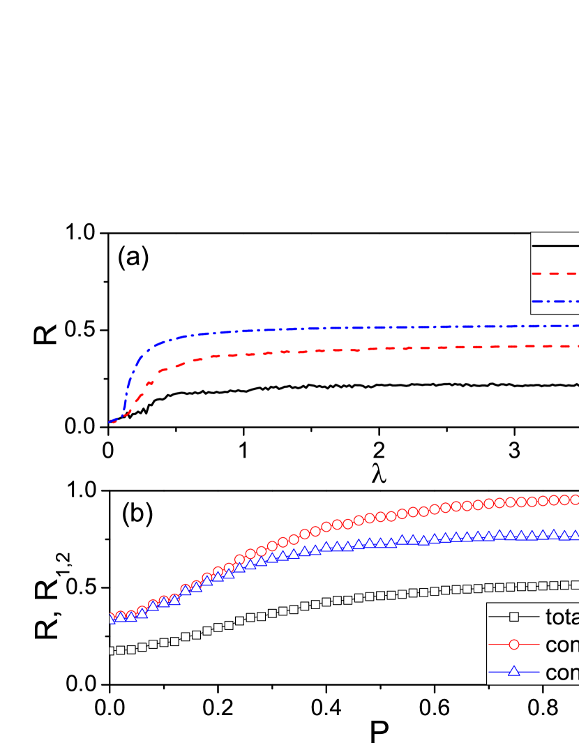
In numerical simulations, we first take the random Erdos-Renyi (ER) network with the average degree $\langle k\rangle=6$ as an example. We let the frequency $\omega_{i}$ in Eq. (1) satisfy the Lorentzian distribution of $g(\omega)=\frac{1}{\pi}[\frac{\gamma}{(\omega-\omega_{0})^{2}+\gamma^{2}}]$ with the central frequency $\omega_{0}$ and $\gamma$ is the half width at half maximum Matthews:1991 . We let the parameters be $N=1000$, $\omega_{0}=0$, $\gamma=0.2$ and $\rho=0.25$ in this paper. Fig. 1(a) shows how $R$ changes with $\lambda$ where the “solid”, “dashed”, and “dash-dotted” lines represent the cases of $P=0,0.4$, and $0.8$, respectively. It is easy to see that the three lines are overlapped when $\lambda$ is very small and then they quickly separated when $\lambda$ is gradually increased. The “squares” in Fig. 1(b) shows how $R$ depends on $P$. We see that $R$ gradually increases with $P$, indicating that the tit-for-tat strategy can successfully suppress the negative role of contrarians in synchronization.

Figure 1: (color online). Synchronization diagrams by the tit-for-tat strategy. (a) $R$ versus $\lambda$ where the “solid”, “dashed”, and “dash-dotted” lines represent the cases of $P=0,0.4$, and $0.8$, respectively. (b) $R,R_{1}$ and $R_{2}$ versus $P$ for $\lambda=3.0$, where the lines with “squares”, “circles”, and “triangles” represent the cases of the total oscillators, the group of conformists, and the group of contrarians, respectively.

To reveal the underlying mechanism of tit-for-tat strategy, we introduce two new order parameters $R_{1}$ and $R_{2}$ defined by

$$R_{1}e^{i\Psi_{1}}=\frac{1}{(1-\rho)N}\sum_{j=1}^{(1-\rho)N}e^{i\theta_{j}}$$ (3)

for the group of conformists and

$$R_{2}e^{i\Psi_{2}}=\frac{1}{\rho N}\sum_{j=1}^{\rho N}e^{i\theta_{j}}$$ (4)

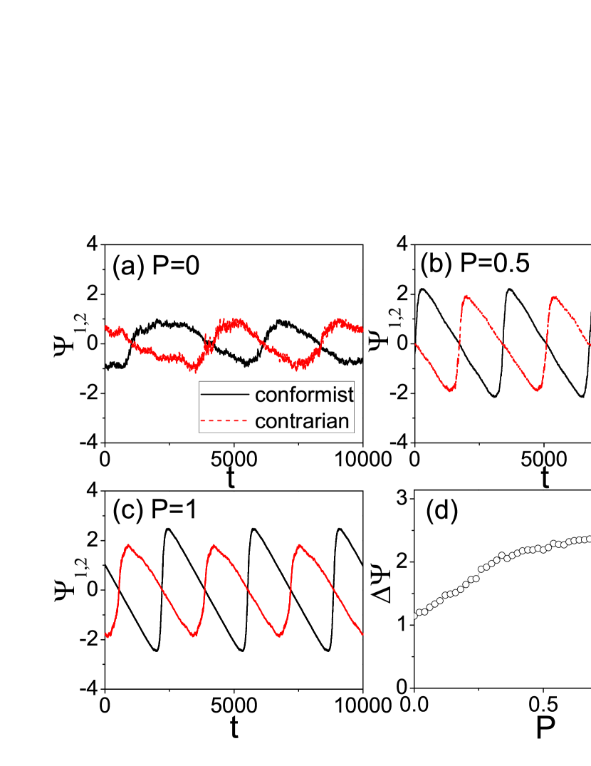
for the group of contrarians. The lines with “circles” and “triangles” in Fig. 1(b) represent the dependence of $R_{1}$ and $R_{2}$ on $P$, respectively. It is easy to see that both $R_{1}$ and $R_{2}$ increase with $R$ and are much larger than the corresponding total $R$. Especially, $R_{1}$ will be close to unity when $P>0.6$, indicating that most of the conformists has become synchronized. To understand the relationship between the conformists and contrarians, Fig. 2 shows how the parameter $P$ influences the evolution of the average phases $\Psi_{1}$ and $\Psi_{2}$ in Eqs. (3) and (4) and where (a)-(c) represent the cases of $P=0,0.5$ and $1$, respectively, and (d) represents the dependence of $\Delta\Psi$ on $P$ with $\Delta\Psi=\langle|\Psi_{1}-\Psi_{2}|\rangle$. From Fig. 2(d) we see that $\Delta\Psi$ increases with $P$ and approaches $\pi$ when $P$ is relatively large, indicating that the tit-for-tat strategy has made the conformists and contrarians become two independent synchronized groups with a phase difference close to $\pi$. Substituting this result into Eq. (2), we find that the two groups of conformists and contrarians will have the opposite contributions to the order parameter $R$ and thus make the value of $R$ in Fig. 1(b) much less than the corresponding $R_{1}$ and $R_{2}$.

Figure 2: (color online). Evolution of the average phases $\Psi_{1}$ and $\Psi_{2}$ where (a)-(c) represent the cases of $P=0,0.5$ and $1$, respectively, and (d) represents the dependence of $\Delta\Psi$ on $P$.

To understand the phase difference $\Delta\Psi$ better, we introduce the link frustration $f_{ij}$ for a connected link $i-j$ as follows Zanette:2005 ; Levnajic:2011

$$f_{ij}=\cos(\theta_{i}-\theta_{j}),$$ (5)

which represents the local dynamical information. Depending on the property of nodes $i$ and $j$, $f_{ij}$ can be classified into three classes of conformist-conformist, conformist-contrarian, and contrarian-contrarian. Those links of conformist-contrarian denote the connections between the two groups of conformists and contrarians and thus represent the asymmetric interaction between the positive and negative couplings. The global frustration can be defined as the network average of $f_{ij}$

$$F=\frac{\sum_{i=1}^{N}\sum_{j=1}^{N}|A_{ij}|f_{ij}}{\sum_{i=1}^{N}\sum_{j=1}^{N}|A_{ij}|}.$$ (6)

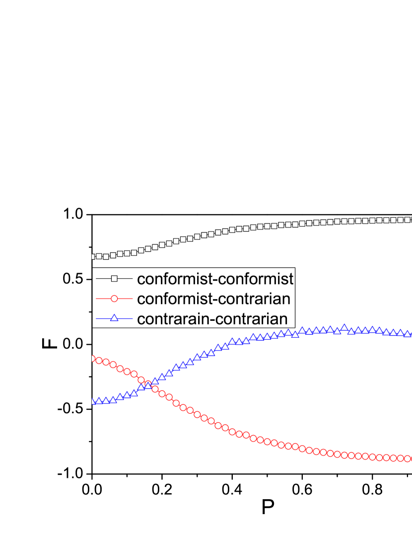
Fig.3 shows the dependence of $F$ on $P$ where the three curves with “squares”, “circles” and “triangles” represent the frustration on the links of conformist-conformist, conformist-contrarian, and contrarian-contrarian, respectively. From Fig.3 we see that with the increase of $P$, $F$ will approach $1,-1,$ and $0$ for the three classes of conformist-conformist, conformist-contrarian, and contrarian-contrarian, respectively. It is not difficult to understand the two cases of $F\approx 1$ and $-1$ as we have $\Delta\Psi\approx 0$ for the links of conformist-conformist with attractive coupling and $\Delta\Psi\approx\pm\pi$ for the links of conformist-contrarian with repulsive coupling. The case of $F\approx 0$ implies $\Delta\Psi\approx\pm\pi/2$, indicating that the group of contrarian-contrarian is not highly synchronized.

Figure 3: (color online). Frustration $F$ versus $P$ where the three curves with “squares”, “circles” and “triangles” represent the frustration on the links of conformist-conformist, conformist-contrarian, and contrarian-contrarian, respectively.

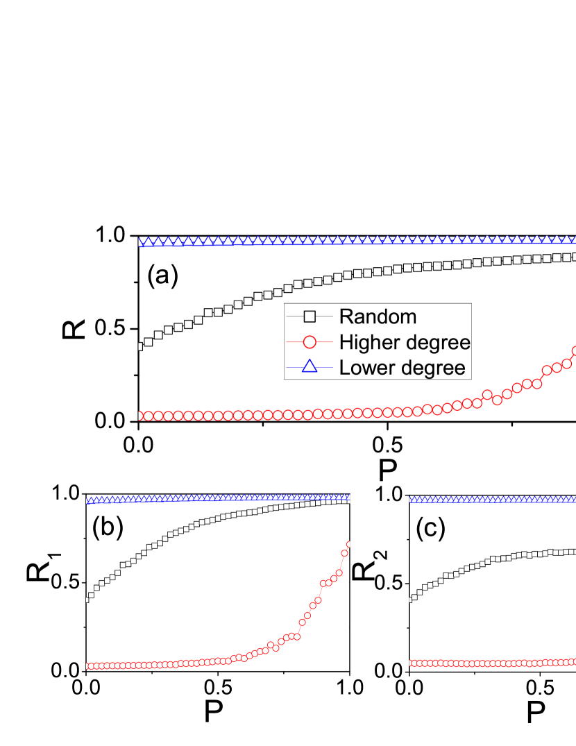
To check the influence of network topology, we now turn to a scale-free network according to the algorithm given by Barabasi-Albert (BA) Barabasi:1999 , where the other parameters are remained the same as in the case of ER network. In contrast to the homogeneous degree distribution in the ER network, the BA network is heterogeneous with a power-law degree distribution. Thus, except the random uniformly choosing the contrarian nodes, we also consider the cases of choosing only those nodes with larger degrees or smaller degrees as contrarians. Fig. 4 shows the results where the three curves with “squares”, “circles” and “triangles” represent the cases of choosing nodes of contrarians by random, the higher degrees and lower degrees, respectively, and (a)-(c) denote the cases of $R$, $R_{1}$ and $R_{2}$, respectively. Comparing the curves with “squares” in Fig. 4(a)-(c) with the corresponding curves in Fig. 1(b), respectively, we find that they are similar, indicating that the tit-for-tat strategy also works for the BA network. Then we notice that all the curves with “triangles” in Fig. 4(a)-(c) are approximate constant, implying that the nodes with lower degrees are not very important. However, we also notice that all the curves with “circles” in Fig. 4(a)-(c) are sensitive on $P$ only when $P>0.5$. The mechanism can be explained as follows. A characteristic feature of the BA network is that the hubs have a large number of links while the leaves have a few links. When the contrarians are chosen from the leaves, the links of conformist-contrarian will be small and thus their influence through the tit-for-tat strategy is also small, resulting the approximate constant curves with “triangles” in Fig. 4. When the contrarians are chosen from the hubs, the links of conformist-contrarian will be large. However, as most of the neighbors of a hub are leaves, it is very possible for those links of hub-leaves to be chosen for the tit-for-tat strategy when $P<0.5$. We know that the leaves will not take an important role in the collective behaviors, thus resulting in the insensitive on $P$ in the curves with “circles” in Fig. 4 for $P<0.5$. When $P>0.5$, the possibility to choose those links of hub-hub or hub-middle nodes for the tit-for-tat strategy will gradually increase, resulting in the sensitive on $P$ in the curves with “circles” in Fig. 4 for $P>0.5$. Similarly, we can understand the case of choosing the contrarians randomly, i.e. the curves with “squares” in Fig. 4.

Figure 4: (color online). Case of BA network corresponding to Fig. 1(b) where the three curves with “squares”, “circles” and “triangles” represent the cases of choosing nodes of contrarians by random, the higher degrees and lower degrees, respectively. (a) $R$ versus $P$; (b) $R_{1}$ versus $P$; (c) $R_{2}$ versus $P$.

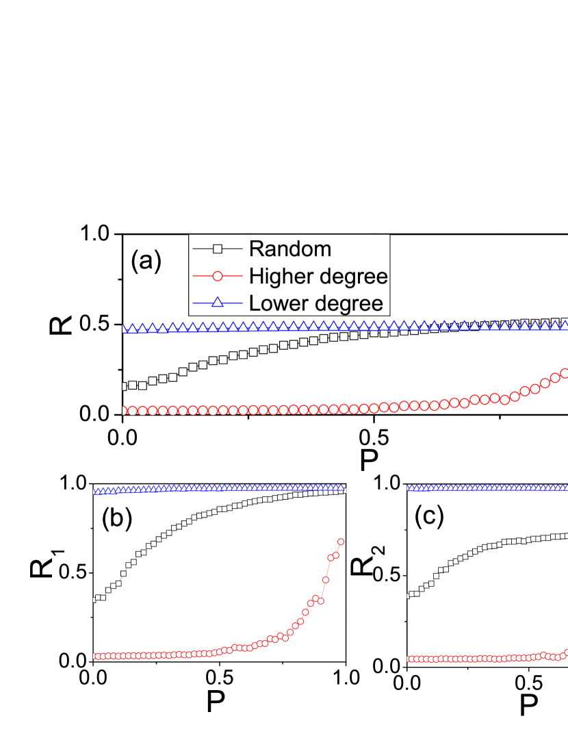
In sum, the case of random uniformly distributed contrarians is much more sensitive to $P$, in contrast to the two cases of choosing the nodes of higher and lower degrees as contrarians, indicating that the tit-for-tat strategy may be more efficient when the contrarians are random uniformly mixed. This result is a little counterintuitive as we usually think that it would be more efficient to choose the nodes of higher degrees as contrarians. Thus, this finding is of interesting as it may have some applications. For example, in the case of epidemic spreading, people are more easy to be vaccinated when the contrarians are random distributed. For the same reason, in the political election, a final winner can be easier to be generated when the contrarians are random distributed.

III Case II: contrarian oscillators sending negative coupling to their neighbors

In this case, Eq. (1) will be replaced by the following equation

$$\dot{\theta_{i}}=\omega_{i}+\lambda\sum_{j=1}^{N}B_{ij}\sin(\theta_{j}-\theta_{i}),\quad i=1,\ldots,N$$ (7)

where $\lambda$ is the coupling strength of all the oscillators, and $B_{ij}=1$ when the connected neighboring node $j$ is conformist and $B_{ij}=-1$ when the connected neighboring node $j$ is contrarian. A distinguished difference between Eq. (1) and Eq. (7) is that in Eq. (1), all the neighbors of node $i$ are in the same position. While in Eq. (7), the neighbors of node $i$ are in different positions, i.e. the conformist neighbors have positive contribution while the contrarian neighbors have negative contribution. We keep the other parameters and the tit-for-tat strategy the same as in Case I. That is, we let all the asymmetric couplings of $B_{ij}=-B_{ij}$ become symmetric ones of $B_{ij}=B_{ij}=-1$ by a probability $P$, i.e. the tit-for-tat strategy.

In numerical simulations, we first take the random ER network with the same parameters as in Case I as an example. Fig. 5 shows the results corresponding to Fig. 1. From Fig. 5(b) we see that all the three curves gradually increase with $P$, indicating the efficiency of the tit-for-tat strategy. Comparing Fig. 1 with Fig. 5, we see that they have two differences: (1) All the curves in Fig. 5 are higher than the corresponding ones in Fig. 1, indicating that the tit-for-tat strategy is more effective in Case II than in Case I. (2) When $P<0.2$, all the three curves in Fig. 5 are overlapped but separated in Fig. 1. This is because the coupling term in Eq. (7) is only determined by the neighbors of node $i$ no matter node $i$ is a conformist or a contrarian. When $P=0$, Eq. (7) will be statistically the same for both a conformist and a contrarian and thus results in the overlap in Fig. 5(b). While the coupling term in Eq. (1) is determined not only by the neighbors of node $i$ but also by node $i$ itself, which results in a difference between the conformists and the contrarians and thus the separation in Fig. 1(b).

Figure 5: (color online). Case II: Synchronization diagrams by the tit-for-tat strategy. (a) $R$ versus $\lambda$ where the “solid”, “dashed”, and “dash-dotted” lines represent the cases of $P=0,0.4$, and $0.8$, respectively. (b) $R$ and $R_{1,2}$ versus $P$ for $\lambda=3.0$, where the lines with “squares”, “circles”, and “triangles” represent the cases of the total oscillators, the group of conformists, and the group of contrarians, respectively.

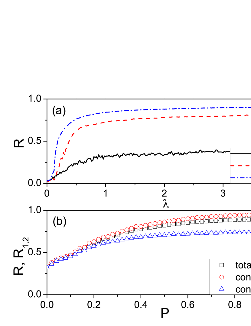
Fig. 6 shows the influence of $P$ on the evolution of the average phases $\Psi_{1}$ and $\Psi_{2}$, corresponding to Fig. 2. Comparing the corresponding curves in Fig. 6 with that in Fig. 2, we observe that $\Delta\Psi$ is close to zero in Fig. 6 but close to $\pi$ in Fig. 2, indicating that the conformists and contrarians will become two independent synchronized groups in Case I but stay in the same synchronized group in Case II.

Figure 6: (color online). Case II: Evolution of the average phases $\Psi_{1}$ and $\Psi_{2}$ where (a)-(c) represent the cases of $P=0,0.5$ and $1$, respectively, and (d) represents the dependence of $\Delta\Psi$ on $P$.

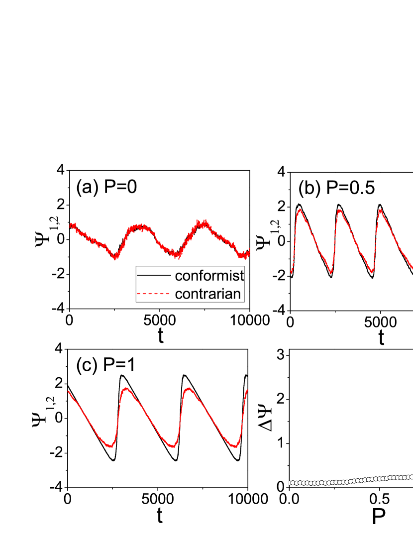
Fig.7 shows the dependence of $F$ on $P$, corresponding to Fig.3. From Fig.7 we see that with the increase of $P$, $F$ will approach $1,1,$ and $0$ for the three classes of conformist-conformist, conformist-contrarian, and contrarian-contrarian, respectively. Comparing Fig.7 with Fig.3 we see that the two classes of conformist-conformist and contrarian-contrarian are similar between the Case I and Case II while the class of conformist-contrarian changes from $F\approx-1$ in Fig.3 to $F\approx 1$ in Fig.7. This point can be understood as follows: In Case I, the formed two synchronized groups have a phase difference $\pi$ and thus the two nodes of a link with conformist-contrarian have a phase difference $\pi$ or opposite phase, which results in $F\approx-1$. While in Case II, both the conformists and contrarians are in the same synchronized group, which results in $F\approx 1$.

Figure 7: (color online). Case II: Frustration $F$ versus $P$ where the three curves with “squares”, “circles” and “triangles” represent the frustration on the links of conformist-conformist, conformist-contrarian, and contrarian-contrarian, respectively.

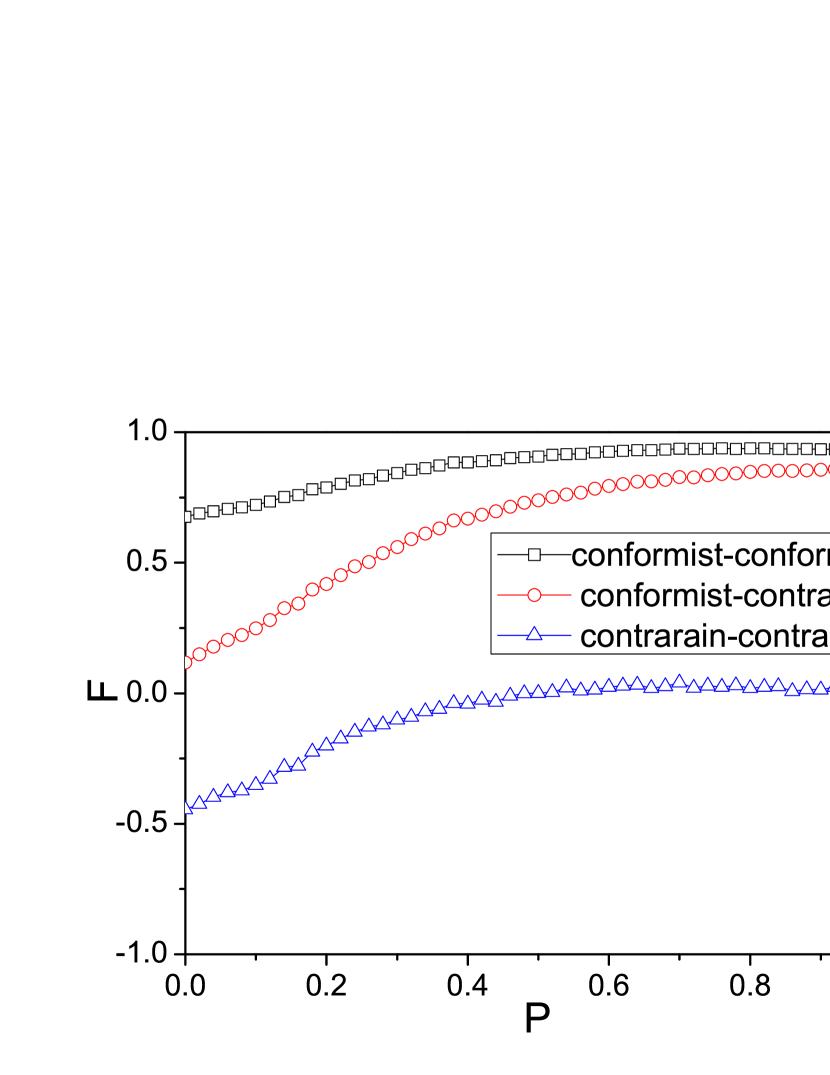
Fig. 8 shows the results of BA network corresponding to Fig. 4, where the three curves with “squares”, “circles” and “triangles” represent the cases of choosing nodes of contrarians by random, the higher degrees and lower degrees, respectively. Comparing the three panels of Fig. 8 with the corresponding ones of Fig. 4, we see that the corresponding panels (b) and (c) are similar each other while all the curves in panel (a) of Fig. 8 are approximate two times of that in panel (a) of Fig. 4, confirming that (1) there is one synchronized group in Case II and two synchronized groups in Case I; and (2) the tit-for-tat strategy is more efficient for the case of random uniformly distributed contrarians.

Figure 8: (color online). Case II: Case of BA network corresponding to Fig. 5(b) where the three curves with “squares”, “circles” and “triangles” represent the cases of choosing nodes of contrarians by random, the higher degrees and lower degrees, respectively. (a) $R$ versus $P$; (b) $R_{1}$ versus $P$; (c) $R_{2}$ versus $P$.

IV A brief theoretical analysis

To understand the role of tit-for-tat strategy better, we here present a brief theoretical analysis. For the convenience of analysis, we rewrite Eq. (1) and Eq. (7) in a unified framework

$$\dot{\theta_{i}}=\omega_{i}+\lambda\sum_{j=1}^{N}C_{ij}\sin(\theta_{j}-\theta_{i}),\quad i=1,\ldots,N$$ (8)

with $\lambda>0$. For Case I, we have $C_{ij}=A_{ij}=1$ when node $i$ is a conformist and $C_{ij}=-A_{ij}=-1$ when node $i$ is a contrarian. For Case II, we always have $C_{ij}=B_{ij}$. We follow the Ref. Restrepo:2005 to introduce a local order parameter $r_{i}$ to quantify the coherence of the inputs to a given node $i$, which is defined by

$$r_{i}e^{i\Psi_{i}}=\sum_{j=1}^{N}C_{ij}\langle e^{i\theta_{j}}\rangle_{t},$$ (9)

where $\langle\cdots\rangle_{t}$ denotes a time average. The right side of Eq. (9) can be divided into two parts: one from the conformist neighbors and the other from the contrarian neighbors. Thus, we rewrite Eq. (9) as

$$r_{i}e^{i\Psi_{i}}=\sum_{j\in conformists}C_{ij}\langle e^{i\theta_{j}}\rangle_{t}+\sum_{j\in contrarians}C_{ij}\langle e^{i\theta_{j}}\rangle_{t}$$ (10)

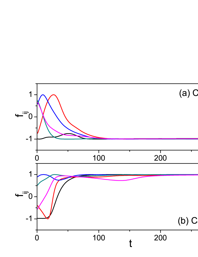
The links of conformist-contrarian are the key elements in Eq. (10) as the tit-for-tat strategy is applied only on them. We here take the case of $P=1$ as an example. For Case I, we first discuss the case of a conformist node $i$. Before using the tit-for-tat strategy, all the $C_{ij}$ in Eq. (10) are positive. After using the tit-for-tat strategy, the $C_{ij}$ in the second term of the right side of Eq. (10) will become negative. The competition between the two terms in the right side of Eq. (10) will depend on their phase differences, which can be reflected by the link frustration of Eq. (5). To figure out the phase differences, Fig. 9(a) shows the evolution of the link frustration $f_{ij}$ with $P=1$ for several typical links of conformist-contrarian in the ER network. From Fig. 9(a) we see that after the transient process, all the $f_{ij}$ will become approximately $-1$, implying that the two terms in the right side of Eq. (10) will have a phase difference $\pi$. That is, the two terms in the right side of Eq. (10) become two synchronized groups with a phase difference $\pi$. Considering one more fact that the values of $C_{ij}$ in the two synchronized groups are $\pm 1$, we see that the negative $C_{ij}$ and the phase difference $\pi$ in the second term of the right side of Eq. (10) will make it have the same positive contribution as the first term of the right side of Eq. (10), and thus enhance the local order parameter $r_{i}$.

Figure 9: (color online). Evolution of the link frustration $f_{ij}$ for several typical links of conformist-contrarian in the ER network when $P=1$. (a) $f_{ij}$ versus $t$ for Case I. (b) $f_{ij}$ versus $t$ for Case II.

The enhanced $r_{i}$ will then make the $r_{i}$ of a contrarian node $i$ increase. That is, all the $r_{i}$ will increase with $P$. In the global level, the order parameter $R$ can be expressed as Restrepo:2005

$$R=\frac{\sum_{i=1}^{N}r_{i}}{\sum_{i=1}^{N}\sum_{j=1}^{N}|A_{ij}|}$$ (11)

Thus, the enhanced $r_{i}$ will make $R$ increase with $P$, which explains the numerical results of Fig. 1.

For Case II, we first discuss the case of a contrarian node $i$. Before using the tit-for-tat strategy, the $C_{ij}$ in the first term of the right side of Eq. (10) is positive while the $C_{ij}$ in the second term of the right side of Eq. (10) is negative. After using the tit-for-tat strategy, the $C_{ij}$ in the first term of the right side of Eq. (10) will become negative, i.e. all the $C_{ij}$ in Eq. (10) are negative now. To figure out the phase differences between the two terms of the right side of Eq. (10), Fig. 9(b) shows the evolution of the link frustration $f_{ij}$ with $P=1$ for several typical links of conformist-contrarian in the ER network. From Fig. 9(b) we see that after the transient process, all the $f_{ij}$ will become approximately $+1$, implying that the two terms in the right side of Eq. (10) will have no phase difference. That is, the two terms in the right side of Eq. (10) become one synchronized group and thus have the same contribution to the synchronization, which enhances the local order parameter $r_{i}$. The enhanced $r_{i}$ will then make the $r_{i}$ of a conformist node $i$ increase. That is, all the $r_{i}$ will increase with $P$ and thus make $R$ of Eq. (11) increase with $P$, which explains the numerical results of Fig. 5.

V Discussions and conclusions

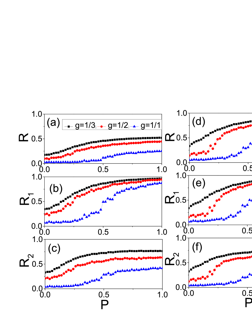
Although all the above discussions are based on $\rho=0.25$, we find that the obtained results also work for other $\rho$. To show this point in detail, we let $g$ be the ratio between the contrarians and conformists, which gives $g\equiv\frac{\rho N}{(1-\rho)N}=\frac{1}{3}$ for $\rho=0.25$. Figure 10 shows how $g$ influences $R,R_{1}$ and $R_{2}$ where the “squares”, “circles” and “triangles” represent the cases of $g=1/3,1/2$ and $1/1$, respectively, and (a)-(c) denote the Case I and (d)-(e) denote the Case II. From Fig. 10 we see that all the three quantities $R,R_{1}$ and $R_{2}$ increase with $P$, no matter it is the Case I or Case II. Thus, the tit-for-tat strategy also works for other $g$ or $\rho$. On the other hand, from Fig. 10 we notice that all the curves with $g=1/3$ are above than that of $g=1/2$ and then both of them are above that of $g=1/1$, indicating that $R,R_{1}$ and $R_{2}$ decrease with the increase of $g$.

Figure 10: (color online). How the ratio $g$ between the contrarians and conformists influences $R,R_{1}$ and $R_{2}$ where the “squares”, “circles” and “triangles” represent the cases of $g=1/3,1/2$ and $1/1$, respectively, and (a)-(c) denote the Case I and (d)-(e) denote the Case II.

The strategy of tit-for-tat is widely used in animal and social competition and is proved to be an efficient way to reach a result of cooperation. The explanation of its microscopic mechanism results in a famous minority game theory based on payoff. In this paper, we first time apply this strategy to the networked systems of coupled oscillators. We reveal that the tit-for-tat strategy takes effect through two elements of the links of conformist-contrarian, i.e. the phase difference and symmetry of the two couplings. The degree of the variation of these two elements will result in different order parameter $R$ for synchronization. This finding is of meaningful in explaining how the neurons network with excitable and inhibitory neurons implements a diversity of cognitive processes, which is closely related to the degree of synchronization.

We notice from both Fig.3 and Fig.7 that the value of $F$ for the links of contrarian-contrarian is approximately zero when $P>0.5$, indicating that the phase difference between two contrarians is about $\pi/2$. This result tells us that a contrarian is always repulsive and thus it is difficult to reach a complete synchronized group of contrarians with $R_{2}=1$. Therefore, an effective way to increase $R$ is to reduce the fraction of contrarian-contrarian interaction, i.e. avoiding two contrarians to be the nearest neighbors.

In conclusions, we have studied the synchronization of a networked system with both positive and negative couplings. We reveal that the negative role of repulsive oscillators to synchronization can be effectively reduced by applying a tit-for-tat strategy. Two kinds of negative couplings are considered and it is found that the tit-for-tat strategy works for both of them. The underlying mechanism is to use the tit-for-tat strategy to against the phase difference of the links of conformist-contrarian and thus increase the synchronization. This result may provide new insights to the diversity of cognitive processes.

This work was partially supported by the NNSF of China under Grant No. 11135001 and 973 Program under Grant No. 2013CB834100.

References

- (1) R. Albert and A.-L. Barabási, Rev. Mod. Phys. 74, 47 (2002).
- (2) S. N. Dorogovtsev, A.V. Goltsev, and J. F. F. Mendes. Rev. Mod. Phys. 80, 1275 (2008).
- (3) A. Arenas, A. Diaz-Guilera, J. Kurths, Y. Moreno, and C. Zhou, Phys. Rep. 469, 93 (2008).
- (4) V. H. P. Louzada, N. A. M. Araujo, J. S. Andrade, Jr. and H. J. Herrmann, Sci. Rep. 2, 658 (2012).
- (5) H. Hong and S. H. Strogatz, Phys. Rev. Lett. 106, 054102 (2011).
- (6) H. Hong and S. H. Strogatz, Phys. Rev. E 84, 046202 (2011).
- (7) C. Borgers and N. Kopell, Neural Comput. 15, 509 (2003).
- (8) J. G. Restrepo, E. Ott, B. R. Hunt, CHAOS 16, 015107 (2005).
- (9) D. H. Zanette, Europhys. Lett., 72, 190 (2005).
- (10) , H. Daido, Phys. Rev. Lett. 68, 1073 (1992).
- (11) L. L. Bonilla, C. J. P. Vicente, and J. M. Rubi, J. Stat. Phys. 70, 921 (1993).
- (12) J. Soriano, M. R. Martinez, T. Tlusty, and E. Moses, Proc. Natl. Acad. Sci. U.S.A. 105, 13758 (2008).
- (13) T. P. Vogels and L. F. Abbott, Nat. Neurosci. 12, 483 (2009).
- (14) J. F. Hipp, A. K. Engel, and M. Siegel, Neuron 69, 387 (2011).
- (15) P. R. Roelfsema and A. k. Engel, Nature 385, 157 (1997)
- (16) T. P. Vogels and L. F. Abbott, J. Neurosci. 25, 10786 (2005).
- (17) M. Diesmann, M. Gewaltig, and A. Aertsen, Nature 402, 529 (1999).
- (18) W. Singer, Neuron 24, 49 (1999).
- (19) T. Womelsdorf, J. M. Schoffelen, R. Oostenveld, W. Singer, R. Desimone, et al., Science 316, 1578 (2007).
- (20) C. Akcay, W. E. Wood, W. A. Searcy, C. N. Templeton, S. E. Campbell, and M.l D. Beecher, Anim. Behav. 78, 97 (2009).
- (21) U. M. Kramer, H. Jansma, C.s Tempelmann, and T. F. Munte, NeuroImage 38, 203 (2007).
- (22) M. Basler, B. T. Ho, and J. J. Mekalanos, Cell 152, 884 (2013).
- (23) R. Axelrod and W. D. Hamilton, Science 211, 1390 (1981).
- (24) M. Milinski, Nature 325, 433 (1987).
- (25) R. Godard, Behav. Ecol. Sociobiol. 33, 45 (1993).
- (26) J. Gómez-Gardeñes, S. Gómez, A. Arenas and Y. Moreno, Phys. Rev. Lett. 106, 128701 (2011).
- (27) P. C. Matthews, R. E. Mirollo and S. H. Strogatz, Physica D 52, 293 (1991).
- (28) Z. Levnajic, Phys. Rev. E 84, 016231 (2011).
- (29) A.-L. Barabasi and R. Albert, Science 286, 509 (1999).