Model-based reinforcement learning in differential graphical gamesthanks: Rushikesh Kamalapurkar, is with the School of Mechanical and Aerospace Engineering, Oklahoma State University, Stillwater, OK, USA. Email: rushikesh.kamalapurkar@okstate.edu. Justin R. Klotz, Patrick Walters, and Warren E. Dixon are with the Department of Mechanical and Aerospace Engineering, University of Florida, Gainesville, FL, USA. Email: {jklotz, walters8, wdixon}@ufl.edu.thanks: This research is supported in part by National Science Foundation award numbers 1217908 and 1509516, and Office of Naval Research award numbers N00014-13-1-0151 and N00014-16-1-2091. Any opinions, findings and conclusions or recommendations expressed in this material are those of the authors and do not necessarily reflect the views of the sponsoring agency.

Rushikesh Kamalapurkar, Justin R. Klotz, Patrick Walters, and Warren E. Dixon
Abstract

This paper seeks to combine differential game theory with the actor-critic-identifier architecture to determine forward-in-time, approximate optimal controllers for formation tracking in multi-agent systems, where the agents have uncertain heterogeneous nonlinear dynamics. A continuous control strategy is proposed, using communication feedback from extended neighbors on a communication topology that has a spanning tree. A model-based reinforcement learning technique is developed to cooperatively control a group of agents to track a trajectory in a desired formation. Simulation results are presented to demonstrate the performance of the developed technique.

I Introduction

In the past few decades, reinforcement learning (RL)-based techniques have been established as primary tools for online real-time optimization [1, 2, 3, 4, 5, 6, 7]. RL techniques are valuable not only for optimization but also for control synthesis in complex systems such as a distributed network of cognitive agents. Combined efforts from multiple autonomous agents can yield tactical advantages including: improved munitions effects; distributed sensing, detection, and threat response; and distributed communication pipelines [8, 9]. While coordinating behaviors among autonomous agents is a challenging problem that has received mainstream focus, unique challenges arise when seeking optimal autonomous collaborative behaviors. For example, most collaborative control literature focuses on centralized approaches that require all nodes to continuously communicate with a central agent, yielding a heavy communication demand that is subject to failure due to delays, and missing information[10]. Furthermore, the central agent is required to carry enough on-board computational resources to process the data and to generate command signals. These challenges motivate the need to minimize communication for guidance, navigation and control tasks, and to distribute the computational burden among the agents.

Since all the agents in a network have independent collaborative or competitive objectives, the resulting optimization problem is a multi-objective optimization problem. Differential game theory is often used to define optimality in multi-objective optimization problems [11, 12, 13, 14, 15, 16]. For example, a Nash equilibrium solution to a multi-objective optimization problem is said to be achieved if none of the players can benefit from a unilateral deviation from the equilibrium [17]. Thus, Nash equilibrium solutions provide a secure set of strategies in the sense that none of the players have an incentive to diverge from their equilibrium policy. Hence, Nash equilibrium has been a widely used solution concept in differential game-based control techniques. Online real-time solutions to differential games with centralized objectives are presented in results such as [18, 19, 20, 21, 22]; however, since these results solve problems with centralized objectives (i.e., each agent minimizes or maximizes a cost function that penalizes the states of all the agents in the network), they are not applicable for a network of agents with independent decentralized objectives (i.e., each agent minimizes or maximizes a cost function that penalizes only the error states corresponding to itself).

In this paper, the objective is to obtain an online forward-in-time feedback-Nash equilibrium solution (cf. [23, 24, 25, 26, 27, 28]) to an infinite-horizon formation tracking problem, where each agent desires to follow a mobile leader while the group maintains a desired formation. The agents try to minimize cost functions that penalize their own formation tracking errors and their own control efforts.

Various methods have been developed to solve optimal tracking problems for linear systems. In [29, 30, 31, 32], optimal controllers are developed to cooperatively control agents with linear dynamics. In [33], a differential game-based approach is developed for unmanned aerial vehicles to achieve distributed Nash strategies. In [34], an optimal consensus algorithm is developed for a cooperative team of agents with linear dynamics using only partial information.

For nonlinear systems, a MPC-based approach is presented in [35]; however, no stability or convergence analysis is presented. A stable distributed MPC-based approach is presented in [36] for nonlinear discrete-time systems with known nominal dynamics. Asymptotic stability is proved without any interaction between the nodes; however, a nonlinear optimal control problem needs to be solved at every iteration to implement the controller. An optimal tracking approach for formation control is presented in [37] using single network adaptive critics where the value function is learned offline. Recently, a leader-based consensus algorithm is developed in [38] where exact model of the system dynamics is utilized, and convergence to optimality is obtained under a persistence of excitation condition.

For multi-agent problems with decentralized objectives, the desired action by an individual agent depends on the actions and the resulting trajectories of its neighbors; hence, the error system for each agent is a complex nonautonomous dynamical system. Nonautonomous systems, in general, have non-stationary value functions. Since non-stationary functions are difficult to approximate using parameterized function approximation schemes such as neural networks (NNs), designing optimal policies for nonautonomous systems is challenging.

Since the external influence from neighbors renders the dynamics of each agent nonautonomous, optimization in a network of agents presents challenges similar to optimal tracking problems. Using insights gained from the authors’ previous work on optimal tracking problems [39], this paper develops a model-based RL technique to generate feedback-Nash equilibrium policies online, for agents in a network with cooperative or competitive objectives. In particular, the network of agents is separated into autonomous subgraphs, and the differential game is solved separately on each subgraph.

The primary contribution of this paper is the formulation and online approximate feedback-Nash equilibrium solution of an optimal network formation tracking problem. A relative control error minimization technique is introduced to facilitate the formulation of a feasible infinite-horizon total-cost differential graphical game. Dynamic programming-based feedback-Nash equilibrium solution of the differential graphical game is facilitated via the development of a set of coupled Hamilton-Jacobi (HJ) equations. The developed approximate feedback-Nash equilibrium solution is analyzed using a Lyapunov-based stability analysis to demonstrate ultimately bounded formation tracking in the presence of uncertainties.

II Notation

Throughout the paper, nsuperscript𝑛\mathbb{R}^{n} denotes nlimit-from𝑛n-dimensional Euclidean space, >asubscriptabsent𝑎\mathbb{R}_{>a} denotes the set of real numbers strictly greater than a𝑎a\in\mathbb{R}, and asubscriptabsent𝑎\mathbb{R}_{\geq a} denotes the set of real numbers greater than or equal to a𝑎a\in\mathbb{R}. Unless otherwise specified, the domain of all the functions is assumed to be 0subscriptabsent0\mathbb{R}_{\geq 0}. Functions with domain 0subscriptabsent0\mathbb{R}_{\geq 0} are defined by abuse of notation using only their image. For example, the function x:0n:𝑥subscriptabsent0superscript𝑛x:\mathbb{R}_{\geq 0}\to\mathbb{R}^{n} is defined by abuse of notation as xn𝑥superscript𝑛x\in\mathbb{R}^{n}. By abuse of notation, the state variables are also used to denote state trajectories. For example, the state variable x𝑥x in the equation x˙=f(x)+u˙𝑥𝑓𝑥𝑢\dot{x}=f\left(x\right)+u is also used as x(t)𝑥𝑡x\left(t\right) to denote the state trajectory, i.e., the general solution x:0n:𝑥subscriptabsent0superscript𝑛x:\mathbb{R}_{\geq 0}\to\mathbb{R}^{n} to x˙=f(x)+u˙𝑥𝑓𝑥𝑢\dot{x}=f\left(x\right)+u evaluated at time t𝑡t. Unless otherwise specified, all the mathematical quantities are assumed to be time-varying. Unless otherwise specified, an equation of the form g(x)=f+h(y,t)𝑔𝑥𝑓𝑦𝑡g\left(x\right)=f+h\left(y,t\right) is interpreted as g(x(t))=f(t)+h(y(t),t)𝑔𝑥𝑡𝑓𝑡𝑦𝑡𝑡g\left(x\left(t\right)\right)=f\left(t\right)+h\left(y\left(t\right),t\right) for all t0𝑡subscriptabsent0t\in\mathbb{R}_{\geq 0}, and a definition of the form g(x,y)f(y)+h(x)𝑔𝑥𝑦𝑓𝑦𝑥g\left(x,y\right)\triangleq f\left(y\right)+h\left(x\right) for functions g:A×BC:𝑔𝐴𝐵𝐶g:A\times B\to C, f:BC:𝑓𝐵𝐶f:B\to C and h:AC:𝐴𝐶h:A\to C is interpreted as g(x,y)f(y)+h(x),(x,y)A×Bformulae-sequence𝑔𝑥𝑦𝑓𝑦𝑥for-all𝑥𝑦𝐴𝐵g\left(x,y\right)\triangleq f\left(y\right)+h\left(x\right),\>\forall\left(x,y\right)\in A\times B. The total derivative f(x)x𝑓𝑥𝑥\frac{\partial f\left(x\right)}{\partial x} is denoted by f𝑓\nabla f and the partial derivative f(x,y)x𝑓𝑥𝑦𝑥\frac{\partial f\left(x,y\right)}{\partial x} is denoted by xf(x,y)subscript𝑥𝑓𝑥𝑦\nabla_{x}f\left(x,y\right). An n×n𝑛𝑛n\times n identity matrix is denoted by Insubscript𝐼𝑛I_{n}, n×m𝑛𝑚n\times m matrices of zeros and ones are denoted by 𝟎n×msubscript0𝑛𝑚\mathbf{0}_{n\times m} and 𝟏n×msubscript1𝑛𝑚\mathbf{1}_{n\times m}, respectively, and 𝟏Ssubscript1𝑆\mathbf{1}_{S} denotes the indicator function of the set S𝑆S.

III Graph Theory Preliminaries

Consider a set of N𝑁N autonomous agents moving in the state space nsuperscript𝑛\mathbb{R}^{n}. The control objective is for the agents to maintain a desired formation with respect to a leader. The state of the leader is denoted by x0nsubscript𝑥0superscript𝑛x_{0}\in\mathbb{R}^{n}. The agents are assumed to be on a network with a fixed communication topology modeled as a static directed graph (i.e. digraph).

Each agent forms a node in the digraph. The set of all nodes excluding the leader is denoted by 𝒩={1,N}𝒩1𝑁\mathcal{N}=\left\{1,\cdots N\right\} and the leader is denoted by node 0. If node i𝑖i can receive information from node j𝑗j then there exists a directed edge from the jth𝑗thj\textsuperscript{th} to the i𝑖ith node of the digraph, denoted by the ordered pair (j,i)𝑗𝑖\left(j,i\right). Let E𝐸E denote the set of all edges. Let there be a positive weight aijsubscript𝑎𝑖𝑗a_{ij}\in\mathbb{R} associated with each edge (j,i)𝑗𝑖\left(j,i\right). Note that aij0subscript𝑎𝑖𝑗0a_{ij}\neq 0 if and only if (j,i)E.𝑗𝑖𝐸\left(j,i\right)\in E. The digraph is assumed to have no repeated edges, i.e., (i,i)E,i𝑖𝑖𝐸for-all𝑖\left(i,i\right)\notin E,\forall i, which implies aii=0,isubscript𝑎𝑖𝑖0for-all𝑖a_{ii}=0,\forall i. The neighborhood sets of node i𝑖i are denoted by 𝒩isubscript𝒩𝑖\mathcal{N}_{-i} and 𝒩isubscript𝒩𝑖\mathcal{N}_{i}, defined as 𝒩i{j𝒩(j,i)E}subscript𝒩𝑖conditional-set𝑗𝒩𝑗𝑖𝐸\mathcal{N}_{-i}\triangleq\left\{j\in\mathcal{N}\mid\left(j,i\right)\in E\right\} and 𝒩i𝒩i{i}subscript𝒩𝑖subscript𝒩𝑖𝑖\mathcal{N}_{i}\triangleq\mathcal{N}_{-i}\cup\left\{i\right\}.

To streamline the analysis, an adjacency matrix 𝒜N×N𝒜superscript𝑁𝑁\mathcal{A}\in\mathbb{R}^{N\times N} is defined as 𝒜[aiji,j𝒩]𝒜delimited-[]conditionalsubscript𝑎𝑖𝑗𝑖𝑗𝒩\mathcal{A}\triangleq\left[a_{ij}\mid i,j\in\mathcal{N}\right], a diagonal pinning gain matrix 𝒜0N×Nsubscript𝒜0superscript𝑁𝑁\mathcal{A}_{0}\in\mathbb{R}^{N\times N} is defined as 𝒜0diag([a10,,aN0])subscript𝒜0diagsubscript𝑎10subscript𝑎𝑁0\mathcal{A}_{0}\triangleq\mbox{diag}\left(\left[a_{10},\cdots,a_{N0}\right]\right), an in-degree matrix 𝒟N×N𝒟superscript𝑁𝑁\mathcal{D}\in\mathbb{R}^{N\times N} is defined as 𝒟diag(di),𝒟diagsubscript𝑑𝑖\mathcal{D}\triangleq\mbox{diag}\left(d_{i}\right), where dij𝒩iaijsubscript𝑑𝑖subscript𝑗subscript𝒩𝑖subscript𝑎𝑖𝑗d_{i}\triangleq\sum_{j\in\mathcal{N}_{i}}a_{ij}, and a graph Laplacian matrix N×Nsuperscript𝑁𝑁\mathcal{L}\in\mathbb{R}^{N\times N} is defined as 𝒟𝒜𝒟𝒜\mathcal{L}\triangleq\mathcal{D}-\mathcal{A}. The graph is assumed to have a spanning tree, i.e., given any node i𝑖i, there exists a directed path from the leader 00 to node i𝑖i. A node j𝑗j is said to be an extended neighbor of node i𝑖i if there exists a directed path from node j𝑗j to node i𝑖i. The extended neighborhood set of node i𝑖i, denoted by 𝒮isubscript𝒮𝑖\mathcal{S}_{-i}, is defined as the set of all extended neighbors of node i.𝑖i. Formally, 𝒮i{j𝒩jiκN,{j1,jκ}𝒩{(j,j1),(j1,j2),,(jκ,i)}2E}subscript𝒮𝑖conditional-set𝑗𝒩formulae-sequence𝑗𝑖𝜅𝑁subscript𝑗1subscript𝑗𝜅conditional𝒩𝑗subscript𝑗1subscript𝑗1subscript𝑗2subscript𝑗𝜅𝑖superscript2𝐸\mathcal{S}_{-i}\triangleq\{j\in\mathcal{N}\mid j\neq i\wedge\exists\kappa\leq N,\>\left\{j_{1},\cdots j_{\kappa}\right\}\subset\mathcal{N}\mid\left\{\left(j,j_{1}\right),\left(j_{1},j_{2}\right),\cdots,\left(j_{\kappa},i\right)\right\}\subset 2^{E}\}. Let 𝒮i𝒮i{i}subscript𝒮𝑖subscript𝒮𝑖𝑖\mathcal{S}_{i}\triangleq\mathcal{S}_{-i}\cup\left\{i\right\}, and let the edge weights be normalized such that jaij=1subscript𝑗subscript𝑎𝑖𝑗1\sum_{j}a_{ij}=1 for all i𝒩𝑖𝒩i\in\mathcal{N}. Note that the sub-graphs are nested in the sense that 𝒮j𝒮isubscript𝒮𝑗subscript𝒮𝑖\mathcal{S}_{j}\subseteq\mathcal{S}_{i} for all j𝒮i𝑗subscript𝒮𝑖j\in\mathcal{S}_{i}.

IV Problem Formulation

The state xinsubscript𝑥𝑖superscript𝑛x_{i}\in\mathbb{R}^{n} of each agent evolves according to the control affine dynamics

x˙i=fi(xi)+gi(xi)ui,subscript˙𝑥𝑖subscript𝑓𝑖subscript𝑥𝑖subscript𝑔𝑖subscript𝑥𝑖subscript𝑢𝑖\dot{x}_{i}=f_{i}\left(x_{i}\right)+g_{i}\left(x_{i}\right)u_{i}, (1)

where uimisubscript𝑢𝑖superscriptsubscript𝑚𝑖u_{i}\in\mathbb{R}^{m_{i}} denotes the control input, and fi:nn:subscript𝑓𝑖superscript𝑛superscript𝑛f_{i}:\mathbb{R}^{n}\to\mathbb{R}^{n} and gi:nn×mi:subscript𝑔𝑖superscript𝑛superscript𝑛subscript𝑚𝑖g_{i}:\mathbb{R}^{n}\to\mathbb{R}^{n\times m_{i}} are locally Lipschitz continuous functions.

Assumption 1.

The dynamics of the leader are described by x˙0=f0(x0),subscript˙𝑥0subscript𝑓0subscript𝑥0\dot{x}_{0}=f_{0}\left(x_{0}\right), where f0:nn:subscript𝑓0superscript𝑛superscript𝑛f_{0}:\mathbb{R}^{n}\to\mathbb{R}^{n} is a locally Lipschitz continuous function. The function f0subscript𝑓0f_{0}, and the initial condition x0(t0)subscript𝑥0subscript𝑡0x_{0}\left(t_{0}\right) are selected such that the trajectory x0(t)subscript𝑥0𝑡x_{0}\left(t\right) is uniformly bounded for all tt0𝑡subscriptabsentsubscript𝑡0t\in\mathbb{R}_{\geq t_{0}}.

The control objective is for the agents to maintain a predetermined formation (with respect to an inertial reference frame) around the leader while minimizing their own cost functions. For all i𝒩𝑖𝒩i\in\mathcal{N}, the ith𝑖thi\textsuperscript{th} agent is aware of its constant desired relative position xdijnsubscript𝑥𝑑𝑖𝑗superscript𝑛x_{dij}\in\mathbb{R}^{n} with respect to all its neighbors j𝒩i𝑗subscript𝒩𝑖j\in\mathcal{N}_{-i}, such that the desired formation is realized when xixjxdijsubscript𝑥𝑖subscript𝑥𝑗subscript𝑥𝑑𝑖𝑗x_{i}-x_{j}\to x_{dij} for all i,j𝒩𝑖𝑗𝒩i,j\in\mathcal{N}.111The vectors xdijsubscript𝑥𝑑𝑖𝑗x_{dij} are assumed to be fixed in an inertial reference frame, i.e., the final desired formation is rigid and its motion in an inertial reference frame can be described as pure translation. To facilitate the control design, the formation is expressed in terms of a set of constant vectors {xdi0n}i𝒩subscriptsubscript𝑥𝑑𝑖0superscript𝑛𝑖𝒩\left\{x_{di0}\in\mathbb{R}^{n}\right\}_{i\in\mathcal{N}} where each xdi0subscript𝑥𝑑𝑖0x_{di0} denotes the constant final desired position of agent i𝑖i with respect to the leader. The vectors {xdi0}i𝒩subscriptsubscript𝑥𝑑𝑖0𝑖𝒩\left\{x_{di0}\right\}_{i\in\mathcal{N}} are unknown to the agents not connected to the leader, and the known desired inter agent relative position can be expressed in terms of {xdi0}i𝒩subscriptsubscript𝑥𝑑𝑖0𝑖𝒩\left\{x_{di0}\right\}_{i\in\mathcal{N}} as xdij=xdi0xdj0subscript𝑥𝑑𝑖𝑗subscript𝑥𝑑𝑖0subscript𝑥𝑑𝑗0x_{dij}=x_{di0}-x_{dj0}. The control objective is thus satisfied when xixdi0+x0subscript𝑥𝑖subscript𝑥𝑑𝑖0subscript𝑥0x_{i}\to x_{di0}+x_{0} for all i𝒩𝑖𝒩i\in\mathcal{N}. To quantify the objective, local neighborhood tracking error signals are defined as

ei=j{0}𝒩iaij((xixj)xdij).subscript𝑒𝑖subscript𝑗0subscript𝒩𝑖subscript𝑎𝑖𝑗subscript𝑥𝑖subscript𝑥𝑗subscript𝑥𝑑𝑖𝑗e_{i}=\sum_{j\in\left\{0\right\}\cup\mathcal{N}_{-i}}a_{ij}\left(\left(x_{i}-x_{j}\right)-x_{dij}\right). (2)

To facilitate the analysis, the error signals in (2) are expressed in terms of the unknown leader-relative desired positions as

ei=j{0}𝒩iaij((xixdi0)(xjxdj0)).subscript𝑒𝑖subscript𝑗0subscript𝒩𝑖subscript𝑎𝑖𝑗subscript𝑥𝑖subscript𝑥𝑑𝑖0subscript𝑥𝑗subscript𝑥𝑑𝑗0e_{i}=\sum_{j\in\left\{0\right\}\cup\mathcal{N}_{-i}}a_{ij}\left(\left(x_{i}-x_{di0}\right)-\left(x_{j}-x_{dj0}\right)\right). (3)

Stacking the error signals in a vector [e1T,e2T,,eNT]TnNsuperscriptdelimited-[]superscriptsubscript𝑒1𝑇superscriptsubscript𝑒2𝑇superscriptsubscript𝑒𝑁𝑇𝑇superscript𝑛𝑁\mathcal{E}\triangleq\left[\begin{array}[t]{cccc}e_{1}^{T},&e_{2}^{T},&\cdots,&e_{N}^{T}\end{array}\right]^{T}\in\mathbb{R}^{nN} the equation in (3) can be expressed in a matrix form

=((+𝒜0)In)(𝒳𝒳d𝒳0),tensor-productsubscript𝒜0subscript𝐼𝑛𝒳subscript𝒳𝑑subscript𝒳0\mathcal{E}=\left(\left(\mathcal{L}+\mathcal{A}_{0}\right)\otimes I_{n}\right)\left(\mathcal{X}-\mathcal{X}_{d}-\mathcal{X}_{0}\right), (4)

where 𝒳=𝒳absent\mathcal{X}= [x1T,\left[x_{1}^{T},\right. x2T,superscriptsubscript𝑥2𝑇x_{2}^{T}, ,\cdots, xNT]T\left.x_{N}^{T}\right]^{T}nNabsentsuperscript𝑛𝑁\in\mathbb{R}^{nN}, 𝒳d=subscript𝒳𝑑absent\mathcal{X}_{d}= [xd10T,\left[x_{d10}^{T},\right. xd20T,superscriptsubscript𝑥𝑑20𝑇x_{d20}^{T}, ,\cdots, xdN0T]T\left.x_{dN0}^{T}\right]^{T}nNabsentsuperscript𝑛𝑁\in\mathbb{R}^{nN}, 𝒳0=subscript𝒳0absent\mathcal{X}_{0}= [x0T,\left[x_{0}^{T},\right. x0T,superscriptsubscript𝑥0𝑇x_{0}^{T}, ,\cdots, x0T]T\left.x_{0}^{T}\right]^{T}nNabsentsuperscript𝑛𝑁\in\mathbb{R}^{nN}, and tensor-product\otimes denotes the Kronecker product. Using (4), it can be concluded that provided the matrix ((+𝒜0)In)nN×nNtensor-productsubscript𝒜0subscript𝐼𝑛superscript𝑛𝑁𝑛𝑁\left(\left(\mathcal{L}+\mathcal{A}_{0}\right)\otimes I_{n}\right)\in\mathbb{R}^{nN\times nN} is nonsingular, 0norm0\left\|\mathcal{E}\right\|\to 0 implies xixdi0+x0subscript𝑥𝑖subscript𝑥𝑑𝑖0subscript𝑥0x_{i}\to x_{di0}+x_{0} for all i𝒩𝑖𝒩i\in\mathcal{N}, and hence, the satisfaction of control objective. The matrix ((+𝒜0)In)tensor-productsubscript𝒜0subscript𝐼𝑛\left(\left(\mathcal{L}+\mathcal{A}_{0}\right)\otimes I_{n}\right) is nonsingular provided the graph has a spanning tree with the leader at the root [40]. To facilitate the formulation of an optimization problem, the following section explores the functional dependence of the state-value functions for the network of agents.

IV-A Elements of the value function

The dynamics for the open-loop neighborhood tracking error are e˙i=j{0}𝒩iaij(fi(xi)+gi(xi)uifj(xj)gj(xj)uj).subscript˙𝑒𝑖subscript𝑗0subscript𝒩𝑖subscript𝑎𝑖𝑗subscript𝑓𝑖subscript𝑥𝑖subscript𝑔𝑖subscript𝑥𝑖subscript𝑢𝑖subscript𝑓𝑗subscript𝑥𝑗subscript𝑔𝑗subscript𝑥𝑗subscript𝑢𝑗\dot{e}_{i}=\sum_{j\in\left\{0\right\}\cup\mathcal{N}_{-i}}a_{ij}\Bigl{(}f_{i}\left(x_{i}\right)+g_{i}\left(x_{i}\right)u_{i}-f_{j}\left(x_{j}\right)-g_{j}\left(x_{j}\right)u_{j}\Bigr{)}. Under the temporary assumption that each controller uisubscript𝑢𝑖u_{i} is an error-feedback controller, i.e. ui(t)=u^i(ei(t),t)subscript𝑢𝑖𝑡subscript^𝑢𝑖subscript𝑒𝑖𝑡𝑡u_{i}\left(t\right)=\hat{u}_{i}\left(e_{i}\left(t\right),t\right), the error dynamics are expressed as e˙i=j{0}𝒩iaij(fi(xi)+gi(xi)u^i(ei,t)fj(xj)gj(xj)u^j(ej,t)).subscript˙𝑒𝑖subscript𝑗0subscript𝒩𝑖subscript𝑎𝑖𝑗subscript𝑓𝑖subscript𝑥𝑖subscript𝑔𝑖subscript𝑥𝑖subscript^𝑢𝑖subscript𝑒𝑖𝑡subscript𝑓𝑗subscript𝑥𝑗subscript𝑔𝑗subscript𝑥𝑗subscript^𝑢𝑗subscript𝑒𝑗𝑡\dot{e}_{i}=\sum_{j\in\left\{0\right\}\cup\mathcal{N}_{-i}}a_{ij}\Bigl{(}f_{i}\left(x_{i}\right)+g_{i}\left(x_{i}\right)\hat{u}_{i}\left(e_{i},t\right)-f_{j}\left(x_{j}\right)-g_{j}\left(x_{j}\right)\hat{u}_{j}\left(e_{j},t\right)\Bigr{)}. Thus, the error trajectory {ei(t)}t=t0superscriptsubscriptsubscript𝑒𝑖𝑡𝑡subscript𝑡0\left\{e_{i}\left(t\right)\right\}_{t=t_{0}}^{\infty} , where t0subscript𝑡0t_{0} denotes the initial time, depends on u^j(ej(t),t)subscript^𝑢𝑗subscript𝑒𝑗𝑡𝑡\hat{u}_{j}\left(e_{j}\left(t\right),t\right), j𝒩ifor-all𝑗subscript𝒩𝑖\forall j\in\mathcal{N}_{i}. Similarly, the error trajectory {ej(t)}t=t0superscriptsubscriptsubscript𝑒𝑗𝑡𝑡subscript𝑡0\left\{e_{j}\left(t\right)\right\}_{t=t_{0}}^{\infty} depends on u^k(ek(t),t),k𝒩jsubscript^𝑢𝑘subscript𝑒𝑘𝑡𝑡for-all𝑘subscript𝒩𝑗\hat{u}_{k}\left(e_{k}\left(t\right),t\right),\forall k\in\mathcal{N}_{j}. Recursively, the trajectory {ei(t)}t=t0superscriptsubscriptsubscript𝑒𝑖𝑡𝑡subscript𝑡0\left\{e_{i}\left(t\right)\right\}_{t=t_{0}}^{\infty} depends on u^j(ej(t),t)subscript^𝑢𝑗subscript𝑒𝑗𝑡𝑡\hat{u}_{j}\left(e_{j}\left(t\right),t\right), and hence, on ej(t),j𝒮isubscript𝑒𝑗𝑡for-all𝑗subscript𝒮𝑖e_{j}\left(t\right),\forall j\in\mathcal{S}_{i}. Thus, even if the controller for each agent is restricted to use local error feedback, the resulting error trajectories are interdependent. In particular, a change in the initial condition of one agent in the extended neighborhood causes a change in the error trajectories corresponding to all the extended neighbors. Consequently, the value function corresponding to an infinite-horizon optimal control problem where each agent tries to minimize t0(Q(ei(τ))+R(ui(τ)))𝑑τsuperscriptsubscriptsubscript𝑡0𝑄subscript𝑒𝑖𝜏𝑅subscript𝑢𝑖𝜏differential-d𝜏\intop_{t_{0}}^{\infty}\left(Q\left(e_{i}\left(\tau\right)\right)+R\left(u_{i}\left(\tau\right)\right)\right)d\tau, where Q:n:𝑄superscript𝑛Q:\mathbb{R}^{n}\to\mathbb{R} and R:mi:𝑅superscriptsubscript𝑚𝑖R:\mathbb{R}^{m_{i}}\to\mathbb{R} are positive definite functions, is dependent on the error states of all the extended neighbors.

Since the steady-state controllers required for formation tracking are generally nonzero, quadratic total-cost optimal control problems result in infinite costs, and hence, are infeasible. In the following section, relative steady-state controllers are derived to facilitate the formulation of a feasible optimal control problem.

IV-B Optimal formation tracking problem

When the agents are perfectly tracking the desired trajectory in the desired formation, even though the states of all the agents are different, the time-derivatives of the states of all the agents are identical. Hence, in steady state, the control signal applied by each agent must be such that the time derivatives of the states corresponding to the set of extended neighbors are identical. In particular, the relative control signal uijmisubscript𝑢𝑖𝑗superscriptsubscript𝑚𝑖u_{ij}\in\mathbb{R}^{m_{i}} that will keep node i𝑖i in its desired relative position with respect to node j𝒮i𝑗subscript𝒮𝑖j\in\mathcal{S}_{-i}, i.e., xi=xj+xdijsubscript𝑥𝑖subscript𝑥𝑗subscript𝑥𝑑𝑖𝑗x_{i}=x_{j}+x_{dij}, must be such that the time derivative of xisubscript𝑥𝑖x_{i} is the same as the time derivative of xjsubscript𝑥𝑗x_{j}. Using the dynamics of the agents from (1), and substituting the desired relative positions xj+xdijsubscript𝑥𝑗subscript𝑥𝑑𝑖𝑗x_{j}+x_{dij} for the states xisubscript𝑥𝑖x_{i}, the relative control signals uijsubscript𝑢𝑖𝑗u_{ij} must satisfy

fi(xj+xdij)+gi(xj+xdij)uij=x˙j.subscript𝑓𝑖subscript𝑥𝑗subscript𝑥𝑑𝑖𝑗subscript𝑔𝑖subscript𝑥𝑗subscript𝑥𝑑𝑖𝑗subscript𝑢𝑖𝑗subscript˙𝑥𝑗f_{i}\left(x_{j}+x_{dij}\right)+g_{i}\left(x_{j}+x_{dij}\right)u_{ij}=\dot{x}_{j}. (5)

The relative steady-state control signals can be expressed in an explicit form provided the following assumption is satisfied.

Assumption 2.

The matrix gi(x)subscript𝑔𝑖𝑥g_{i}\left(x\right) is full rank for all i𝒩𝑖𝒩i\in\mathcal{N} and for all xn𝑥superscript𝑛x\in\mathbb{R}^{n}; furthermore, the relative steady-state control signal expressed as uij=fij(xj)+gij(xj)uj,subscript𝑢𝑖𝑗subscript𝑓𝑖𝑗subscript𝑥𝑗subscript𝑔𝑖𝑗subscript𝑥𝑗subscript𝑢𝑗u_{ij}=f_{ij}\left(x_{j}\right)+g_{ij}\left(x_{j}\right)u_{j}, satisfies (5) along the desired trajectory, where fij(xj)gi+(xj+xdij)(fj(xj)fi(xj+xdij))misubscript𝑓𝑖𝑗subscript𝑥𝑗superscriptsubscript𝑔𝑖subscript𝑥𝑗subscript𝑥𝑑𝑖𝑗subscript𝑓𝑗subscript𝑥𝑗subscript𝑓𝑖subscript𝑥𝑗subscript𝑥𝑑𝑖𝑗superscriptsubscript𝑚𝑖f_{ij}\left(x_{j}\right)\triangleq g_{i}^{+}\left(x_{j}+x_{dij}\right)\left(f_{j}\left(x_{j}\right)-f_{i}\left(x_{j}+x_{dij}\right)\right)\in\mathbb{R}^{m_{i}}, gij(xj)gi+(xj+xdij)gj(xj)mi×mjsubscript𝑔𝑖𝑗subscript𝑥𝑗superscriptsubscript𝑔𝑖subscript𝑥𝑗subscript𝑥𝑑𝑖𝑗subscript𝑔𝑗subscript𝑥𝑗superscriptsubscript𝑚𝑖subscript𝑚𝑗g_{ij}\left(x_{j}\right)\triangleq g_{i}^{+}\left(x_{j}+x_{dij}\right)g_{j}\left(x_{j}\right)\in\mathbb{R}^{m_{i}\times m_{j}}, g0(x)0subscript𝑔0𝑥0g_{0}\left(x\right)\triangleq 0 for all xn𝑥superscript𝑛x\in\mathbb{R}^{n}, ui00subscript𝑢𝑖00u_{i0}\equiv 0 for all i𝒩𝑖𝒩i\in\mathcal{N}, and gi+(x)superscriptsubscript𝑔𝑖𝑥g_{i}^{+}\left(x\right) denotes a pseudoinverse of the matrix gi(x)subscript𝑔𝑖𝑥g_{i}\left(x\right) for all xn𝑥superscript𝑛x\in\mathbb{R}^{n} and for all i𝒩𝑖𝒩i\in\mathcal{N}.

Assumption 2 places restrictions on the control-effectiveness matrices. The matrices gi(x)subscript𝑔𝑖𝑥g_{i}\left(x\right) are full rank for a large class of systems including, but not limited to, kinematic wheels and fully actuated Euler-Lagrange systems with invertible inertia matrices. The second part of Assumption 2 requires the existence of a feedback controller that can keep the system on the desired trajectory if the system starts on the desired trajectory. This assumption depends on the systems, the network, the desired formation, and the desired trajectory; hence, insights into its satisfaction are hard to obtain in general. The satisfaction of this assumption needs to be verified on a case-by-case basis. For example, consider a kinematic wheel modeled as

x˙=g(x)u,g(x)=[cos(x3)0sin(x3)001].formulae-sequence˙𝑥𝑔𝑥𝑢𝑔𝑥matrixsubscript𝑥30subscript𝑥3001\dot{x}=g\left(x\right)u,\quad g\left(x\right)=\begin{bmatrix}\cos\left(x_{3}\right)&0\\ \sin\left(x_{3}\right)&0\\ 0&1\end{bmatrix}. (6)

In this case, provided the formation satisfies xdij(3)=0subscript𝑥𝑑𝑖𝑗30x_{dij}\left(3\right)=0, that is, the target formation is such that all the kinematic wheels have the same steering angle, the functions fijsubscript𝑓𝑖𝑗f_{ij} and gijsubscript𝑔𝑖𝑗g_{ij} can be computed as fij=0,subscript𝑓𝑖𝑗0f_{ij}=0, and gij=I2subscript𝑔𝑖𝑗subscript𝐼2g_{ij}=I_{2}. The relative steady-state control is then uij=ujsubscript𝑢𝑖𝑗subscript𝑢𝑗u_{ij}=u_{j}, which satisfies g(xj+xdij)uj=x˙j𝑔subscript𝑥𝑗subscript𝑥𝑑𝑖𝑗subscript𝑢𝑗subscript˙𝑥𝑗g\left(x_{j}+x_{dij}\right)u_{j}=\dot{x}_{j}, and hence, Assumption 2 holds.

To facilitate the formulation of an optimal formation tracking problem, define the control errors μimisubscript𝜇𝑖superscriptsubscript𝑚𝑖\mu_{i}\in\mathbb{R}^{m_{i}} as

μij𝒩i{0}aij(uiuij).subscript𝜇𝑖subscript𝑗subscript𝒩𝑖0subscript𝑎𝑖𝑗subscript𝑢𝑖subscript𝑢𝑖𝑗\mu_{i}\triangleq\sum_{j\in\mathcal{N}_{-i}\cup\left\{0\right\}}a_{ij}\left(u_{i}-u_{ij}\right). (7)

The control errors {μi}subscript𝜇𝑖\left\{\mu_{i}\right\} are treated as the design variables in the remainder of this paper. Since the control errors {μi}subscript𝜇𝑖\left\{\mu_{i}\right\} are designed and the controllers {ui}subscript𝑢𝑖\left\{u_{i}\right\} are implemented in practice, it is essential to invert the relationship in (7). To facilitate the inversion, let 𝒮io{1,,si}superscriptsubscript𝒮𝑖𝑜1subscript𝑠𝑖\mathcal{S}_{i}^{o}\triangleq\left\{1,\cdots,s_{i}\right\}, where si|𝒮i|subscript𝑠𝑖subscript𝒮𝑖s_{i}\triangleq\left|\mathcal{S}_{i}\right|. Let λi:𝒮io𝒮i:subscript𝜆𝑖superscriptsubscript𝒮𝑖𝑜subscript𝒮𝑖\lambda_{i}:\mathcal{S}_{i}^{o}\to\mathcal{S}_{i} be a bijective map such that λi(1)=isubscript𝜆𝑖1𝑖\lambda_{i}\left(1\right)=i. For notational brevity, let ()𝒮isubscriptsubscript𝒮𝑖\left(\cdot\right)_{\mathcal{S}_{i}} denote the concatenated vector [()λi1T,()λi2T,,()λisiT]Tsuperscriptsuperscriptsubscriptsuperscriptsubscript𝜆𝑖1𝑇superscriptsubscriptsuperscriptsubscript𝜆𝑖2𝑇superscriptsubscriptsuperscriptsubscript𝜆𝑖subscript𝑠𝑖𝑇𝑇\left[\left(\cdot\right)_{\lambda_{i}^{1}}^{T},\left(\cdot\right)_{\lambda_{i}^{2}}^{T},\cdots,\left(\cdot\right)_{\lambda_{i}^{s_{i}}}^{T}\right]^{T}, let ()𝒮isubscriptsubscript𝒮𝑖\left(\cdot\right)_{\mathcal{S}_{-i}} denote the concatenated vector [()λi2T,,()λisiT]Tsuperscriptsuperscriptsubscriptsuperscriptsubscript𝜆𝑖2𝑇superscriptsubscriptsuperscriptsubscript𝜆𝑖subscript𝑠𝑖𝑇𝑇\left[\left(\cdot\right)_{\lambda_{i}^{2}}^{T},\cdots,\left(\cdot\right)_{\lambda_{i}^{s_{i}}}^{T}\right]^{T}, let isuperscript𝑖\sum^{i} denote j𝒩i{0}subscript𝑗subscript𝒩𝑖0\sum_{j\in\mathcal{N}_{-i}\cup\left\{0\right\}}, let λijsuperscriptsubscript𝜆𝑖𝑗\lambda_{i}^{j} denote λi(j)subscript𝜆𝑖𝑗\lambda_{i}\left(j\right), let i[e𝒮iT,xλi1T]Tn(si+1)subscript𝑖superscriptsuperscriptsubscript𝑒subscript𝒮𝑖𝑇superscriptsubscript𝑥superscriptsubscript𝜆𝑖1𝑇𝑇superscript𝑛subscript𝑠𝑖1\mathcal{E}_{i}\triangleq\left[e_{\mathcal{S}_{i}}^{T},x_{\lambda_{i}^{1}}^{T}\right]^{T}\in\mathbb{R}^{n\left(s_{i}+1\right)}, and let i[e𝒮iT,xλi1T]Tnsisubscript𝑖superscriptsuperscriptsubscript𝑒subscript𝒮𝑖𝑇superscriptsubscript𝑥superscriptsubscript𝜆𝑖1𝑇𝑇superscript𝑛subscript𝑠𝑖\mathcal{E}_{-i}\triangleq\left[e_{\mathcal{S}_{-i}}^{T},x_{\lambda_{i}^{1}}^{T}\right]^{T}\in\mathbb{R}^{ns_{i}}. Then, the control error vectors μ𝒮ik𝒮imksubscript𝜇subscript𝒮𝑖superscriptsubscript𝑘subscript𝒮𝑖subscript𝑚𝑘\mu_{\mathcal{S}_{i}}\in\mathbb{R}^{\sum_{k\in\mathcal{S}_{i}}m_{k}} can be expressed as

μ𝒮i=gi(i)u𝒮iFi(i),subscript𝜇subscript𝒮𝑖subscript𝑔𝑖subscript𝑖subscript𝑢subscript𝒮𝑖subscript𝐹𝑖subscript𝑖\mu_{\mathcal{S}_{i}}=\mathscr{L}_{gi}\left(\mathcal{E}_{i}\right)u_{\mathcal{S}_{i}}-F_{i}\left(\mathcal{E}_{i}\right), (8)

where the matrices gi:n(si+1)k𝒮imk×k𝒮imk:subscript𝑔𝑖superscript𝑛subscript𝑠𝑖1superscriptsubscript𝑘subscript𝒮𝑖subscript𝑚𝑘subscript𝑘subscript𝒮𝑖subscript𝑚𝑘\mathscr{L}_{gi}:\mathbb{R}^{n\left(s_{i}+1\right)}\to\mathbb{R}^{\sum_{k\in\mathcal{S}_{i}}m_{k}\times\sum_{k\in\mathcal{S}_{i}}m_{k}} are defined by

[gi(i)]kl={aλikλilgλikλil(xλil),lk,λikaλikjImλik,l=k,subscriptdelimited-[]subscript𝑔𝑖subscript𝑖𝑘𝑙casessubscript𝑎superscriptsubscript𝜆𝑖𝑘superscriptsubscript𝜆𝑖𝑙subscript𝑔superscriptsubscript𝜆𝑖𝑘superscriptsubscript𝜆𝑖𝑙subscript𝑥superscriptsubscript𝜆𝑖𝑙for-all𝑙𝑘superscriptsuperscriptsubscript𝜆𝑖𝑘subscript𝑎superscriptsubscript𝜆𝑖𝑘𝑗subscript𝐼subscript𝑚superscriptsubscript𝜆𝑖𝑘for-all𝑙𝑘\left[\mathscr{L}_{gi}\left(\mathcal{E}_{i}\right)\right]_{kl}=\begin{cases}-a_{\lambda_{i}^{k}\lambda_{i}^{l}}g_{\lambda_{i}^{k}\lambda_{i}^{l}}\left(x_{\lambda_{i}^{l}}\right),&\forall l\neq k,\\ \sideset{}{{}^{\lambda_{i}^{k}}}{\sum}a_{\lambda_{i}^{k}j}I_{m_{\lambda_{i}^{k}}},&\forall l=k,\end{cases}

where k,l=1,2,,siformulae-sequence𝑘𝑙12subscript𝑠𝑖k,l=1,2,\cdots,s_{i}, and Fi:n(si+1)k𝒮imk:subscript𝐹𝑖superscript𝑛subscript𝑠𝑖1superscriptsubscript𝑘subscript𝒮𝑖subscript𝑚𝑘F_{i}:\mathbb{R}^{n\left(s_{i}+1\right)}\to\mathbb{R}^{\sum_{k\in\mathcal{S}_{i}}m_{k}} are defined as

Fi(i)[iaλi1jfλi1jT(xj),,λisiaλisijfλisijT(xj)]T.subscript𝐹𝑖subscript𝑖superscriptsuperscript𝑖subscript𝑎superscriptsubscript𝜆𝑖1𝑗superscriptsubscript𝑓superscriptsubscript𝜆𝑖1𝑗𝑇subscript𝑥𝑗superscriptsuperscriptsubscript𝜆𝑖subscript𝑠𝑖subscript𝑎superscriptsubscript𝜆𝑖subscript𝑠𝑖𝑗superscriptsubscript𝑓superscriptsubscript𝜆𝑖subscript𝑠𝑖𝑗𝑇subscript𝑥𝑗𝑇F_{i}\!\left(\!\mathcal{E}_{i}\!\right)\!\triangleq\!\left[\!\sideset{}{{}^{i}}{\sum}\!\!a_{\lambda_{i}^{1}j}f_{\lambda_{i}^{1}j}^{T}\!\left(\!x_{j}\!\right)\!,\!\cdots\!,\!\!\sideset{}{{}^{\lambda_{i}^{s_{i}}}}{\sum}\!\!a_{\lambda_{i}^{s_{i}}j}f_{\lambda_{i}^{s_{i}}j}^{T}\!\left(\!x_{j}\!\right)\!\right]^{T}.
Assumption 3.

The matrix gi(i(t))subscript𝑔𝑖subscript𝑖𝑡\mathscr{L}_{gi}\left(\mathcal{E}_{i}\left(t\right)\right) is invertible for all t𝑡t\in\mathbb{R} and for all i𝒩𝑖𝒩i\in\mathcal{N}.

Assumption 3 is a controllability-like condition. Intuitively, Assumption 3 requires the control effectiveness matrices to be compatible to ensure the existence of relative control inputs that allow the agents to follow the desired trajectory in the desired formation. Assumption 3 depends on the systems, the network, the desired formation, and the desired trajectory; hence, insights into its satisfaction are hard to obtain in general. The satisfaction of this assumption needs to be verified on a case-by-case basis. For example, consider the kinematic wheel in (6). Provided the formation satisfies xdij(3)=0subscript𝑥𝑑𝑖𝑗30x_{dij}\left(3\right)=0, that is, the target formation is such that all the kinematic wheels have the same steering angle, we have gij=I2,subscript𝑔𝑖𝑗subscript𝐼2g_{ij}=I_{2}, and hence, the matrices gisubscript𝑔𝑖\mathscr{L}_{gi} are given by

[gi(i)]kl={aλikλilI2,lk,λikaλikjI2,l=k,subscriptdelimited-[]subscript𝑔𝑖subscript𝑖𝑘𝑙casessubscript𝑎superscriptsubscript𝜆𝑖𝑘superscriptsubscript𝜆𝑖𝑙subscript𝐼2for-all𝑙𝑘superscriptsuperscriptsubscript𝜆𝑖𝑘subscript𝑎superscriptsubscript𝜆𝑖𝑘𝑗subscript𝐼2for-all𝑙𝑘\left[\mathscr{L}_{gi}\left(\mathcal{E}_{i}\right)\right]_{kl}=\begin{cases}-a_{\lambda_{i}^{k}\lambda_{i}^{l}}I_{2},&\forall l\neq k,\\ \sideset{}{{}^{\lambda_{i}^{k}}}{\sum}a_{\lambda_{i}^{k}j}I_{2},&\forall l=k,\end{cases}

It can be shown that gi=𝒮iI2subscript𝑔𝑖tensor-productsubscriptsubscript𝒮𝑖subscript𝐼2\mathscr{L}_{gi}=\mathcal{L}_{\mathcal{S}_{i}}\otimes I_{2}, where 𝒮isubscriptsubscript𝒮𝑖\mathcal{L}_{\mathcal{S}_{i}} denotes the Laplacian matrix corresponding to the subgraph 𝒮isubscript𝒮𝑖\mathcal{S}_{i}. Hence, the graph connectivity condition ensures that the matrices gisubscript𝑔𝑖\mathscr{L}_{gi} are invertible, and in this specific case, Assumption 3 holds.

Using Assumption 3, the control vectors can be expressed as

u𝒮i=gi1(i)μ𝒮i+gi1(i)Fi(i).subscript𝑢subscript𝒮𝑖superscriptsubscript𝑔𝑖1subscript𝑖subscript𝜇subscript𝒮𝑖superscriptsubscript𝑔𝑖1subscript𝑖subscript𝐹𝑖subscript𝑖u_{\mathcal{S}_{i}}=\mathscr{L}_{gi}^{-1}\left(\mathcal{E}_{i}\right)\mu_{\mathcal{S}_{i}}+\mathscr{L}_{gi}^{-1}\left(\mathcal{E}_{i}\right)F_{i}\left(\mathcal{E}_{i}\right). (9)

Let giksuperscriptsubscript𝑔𝑖𝑘\mathscr{L}_{gi}^{k} denote the (λi1(k))superscriptsubscript𝜆𝑖1𝑘\left(\lambda_{i}^{-1}\left(k\right)\right)th block row of gi1superscriptsubscript𝑔𝑖1\mathscr{L}_{gi}^{-1}. Then, the controllers uisubscript𝑢𝑖u_{i} can be implemented as

ui=gii(i)μ𝒮i+gii(i)Fi(i),subscript𝑢𝑖superscriptsubscript𝑔𝑖𝑖subscript𝑖subscript𝜇subscript𝒮𝑖superscriptsubscript𝑔𝑖𝑖subscript𝑖subscript𝐹𝑖subscript𝑖u_{i}=\mathscr{L}_{gi}^{i}\left(\mathcal{E}_{i}\right)\mu_{\mathcal{S}_{i}}+\mathscr{L}_{gi}^{i}\left(\mathcal{E}_{i}\right)F_{i}\left(\mathcal{E}_{i}\right), (10)

and for any j𝒩i𝑗subscript𝒩𝑖j\in\mathcal{N}_{-i},

uj=gij(i)μ𝒮i+gij(i)Fi(i).subscript𝑢𝑗superscriptsubscript𝑔𝑖𝑗subscript𝑖subscript𝜇subscript𝒮𝑖superscriptsubscript𝑔𝑖𝑗subscript𝑖subscript𝐹𝑖subscript𝑖u_{j}=\mathscr{L}_{gi}^{j}\left(\mathcal{E}_{i}\right)\mu_{\mathcal{S}_{i}}+\mathscr{L}_{gi}^{j}\left(\mathcal{E}_{i}\right)F_{i}\left(\mathcal{E}_{i}\right). (11)

Using (10) and (11), the error and the state dynamics for the agents can be represented as

e˙i=i(i)+𝒢i(i)μ𝒮i,subscript˙𝑒𝑖subscript𝑖subscript𝑖subscript𝒢𝑖subscript𝑖subscript𝜇subscript𝒮𝑖\dot{e}_{i}=\mathscr{F}_{i}\left(\mathcal{E}_{i}\right)+\mathscr{G}_{i}\left(\mathcal{E}_{i}\right)\mu_{\mathcal{S}_{i}}, (12)

and

x˙i=i(i)+𝒢i(i)μ𝒮i,subscript˙𝑥𝑖subscript𝑖subscript𝑖subscript𝒢𝑖subscript𝑖subscript𝜇subscript𝒮𝑖\dot{x}_{i}=\mathcal{F}_{i}\left(\mathcal{E}_{i}\right)+\mathcal{G}_{i}\left(\mathcal{E}_{i}\right)\mu_{\mathcal{S}_{i}}, (13)

where

i(i)iaijgi(xi)gii(i)Fi(i)iaijfj(xj)iaijgj(xj)gij(i)Fi(i)+iaijfi(xi),subscript𝑖subscript𝑖superscript𝑖subscript𝑎𝑖𝑗subscript𝑔𝑖subscript𝑥𝑖superscriptsubscript𝑔𝑖𝑖subscript𝑖subscript𝐹𝑖subscript𝑖superscript𝑖subscript𝑎𝑖𝑗subscript𝑓𝑗subscript𝑥𝑗superscript𝑖subscript𝑎𝑖𝑗subscript𝑔𝑗subscript𝑥𝑗superscriptsubscript𝑔𝑖𝑗subscript𝑖subscript𝐹𝑖subscript𝑖superscript𝑖subscript𝑎𝑖𝑗subscript𝑓𝑖subscript𝑥𝑖\mathscr{F}_{i}\left(\mathcal{E}_{i}\right)\triangleq\!\!\sideset{}{{}^{i}}{\sum}a_{ij}g_{i}\left(x_{i}\right)\mathscr{L}_{gi}^{i}\left(\mathcal{E}_{i}\right)F_{i}\left(\mathcal{E}_{i}\right)\!-\!\!\sideset{}{{}^{i}}{\sum}a_{ij}f_{j}\left(x_{j}\right)\\ -\!\!\sideset{}{{}^{i}}{\sum}a_{ij}g_{j}\left(x_{j}\right)\mathscr{L}_{gi}^{j}\left(\mathcal{E}_{i}\right)F_{i}\left(\mathcal{E}_{i}\right)+\!\!\sideset{}{{}^{i}}{\sum}a_{ij}f_{i}\left(x_{i}\right),
𝒢i(i)iaij(gi(xi)gii(i)gj(xj)gij(i)),subscript𝒢𝑖subscript𝑖superscript𝑖subscript𝑎𝑖𝑗subscript𝑔𝑖subscript𝑥𝑖superscriptsubscript𝑔𝑖𝑖subscript𝑖subscript𝑔𝑗subscript𝑥𝑗superscriptsubscript𝑔𝑖𝑗subscript𝑖\mathscr{G}_{i}\left(\mathcal{E}_{i}\right)\triangleq\!\!\sideset{}{{}^{i}}{\sum}a_{ij}\left(g_{i}\left(x_{i}\right)\mathscr{L}_{gi}^{i}\left(\mathcal{E}_{i}\right)-g_{j}\left(x_{j}\right)\mathscr{L}_{gi}^{j}\left(\mathcal{E}_{i}\right)\right),
i(i)fi(xi)+gi(xi)gii(i)Fi(i),subscript𝑖subscript𝑖subscript𝑓𝑖subscript𝑥𝑖subscript𝑔𝑖subscript𝑥𝑖superscriptsubscript𝑔𝑖𝑖subscript𝑖subscript𝐹𝑖subscript𝑖\mathcal{F}_{i}\left(\mathcal{E}_{i}\right)\triangleq f_{i}\left(x_{i}\right)+g_{i}\left(x_{i}\right)\mathscr{L}_{gi}^{i}\left(\mathcal{E}_{i}\right)F_{i}\left(\mathcal{E}_{i}\right),

and 𝒢i(i)gi(xi)gii(i)subscript𝒢𝑖subscript𝑖subscript𝑔𝑖subscript𝑥𝑖superscriptsubscript𝑔𝑖𝑖subscript𝑖\mathcal{G}_{i}\left(\mathcal{E}_{i}\right)\triangleq g_{i}\left(x_{i}\right)\mathscr{L}_{gi}^{i}\left(\mathcal{E}_{i}\right).

Let heiμ¯i,μ¯𝒮i(t,t0,i0)superscriptsubscript𝑒𝑖subscript¯𝜇𝑖subscript¯𝜇subscript𝒮𝑖𝑡subscript𝑡0subscript𝑖0h_{ei}^{\overline{\mu}_{i},\overline{\mu}_{\mathcal{S}_{-i}}}\left(t,t_{0},\mathcal{E}_{i0}\right) and hxiμ¯i,μ¯𝒮i(t,t0,i0)superscriptsubscript𝑥𝑖subscript¯𝜇𝑖subscript¯𝜇subscript𝒮𝑖𝑡subscript𝑡0subscript𝑖0h_{xi}^{\overline{\mu}_{i},\overline{\mu}_{\mathcal{S}_{-i}}}\left(t,t_{0},\mathcal{E}_{i0}\right) denote the trajectories of (12) and (13), respectively, with the initial time t0subscript𝑡0t_{0}, initial condition i(t0)=i0subscript𝑖subscript𝑡0subscript𝑖0\mathcal{E}_{i}\left(t_{0}\right)=\mathcal{E}_{i0}, and policies μ¯j:n(si+1)mi,j𝒮i:subscript¯𝜇𝑗formulae-sequencesuperscript𝑛subscript𝑠𝑖1superscriptsubscript𝑚𝑖𝑗subscript𝒮𝑖\overline{\mu}_{j}:\mathbb{R}^{n\left(s_{i}+1\right)}\to\mathbb{R}^{m_{i}},\>j\in\mathcal{S}_{i}, and let i[(he)𝒮iT,hxλi1T]Tsubscript𝑖superscriptsuperscriptsubscriptsubscript𝑒subscript𝒮𝑖𝑇superscriptsubscript𝑥superscriptsubscript𝜆𝑖1𝑇𝑇\mathcal{H}_{i}\triangleq\left[\left(h_{e}\right)_{\mathcal{S}_{i}}^{T},h_{x\lambda_{i}^{1}}^{T}\right]^{T}. Define the cost functionals

Ji(ei(),μi())0ri(ei(σ),μi(σ))dσsubscript𝐽𝑖subscript𝑒𝑖subscript𝜇𝑖superscriptsubscript0subscript𝑟𝑖subscript𝑒𝑖𝜎subscript𝜇𝑖𝜎d𝜎J_{i}\left(e_{i}\left(\cdot\right),\mu_{i}\left(\cdot\right)\right)\triangleq\intop_{0}^{\infty}r_{i}\left(e_{i}\left(\sigma\right),\mu_{i}\left(\sigma\right)\right)\textnormal{d}\sigma (14)

where ri:n×mi0:subscript𝑟𝑖superscript𝑛superscriptsubscript𝑚𝑖subscriptabsent0r_{i}:\mathbb{R}^{n}\times\mathbb{R}^{m_{i}}\to\mathbb{R}_{\geq 0} denote the local costs defined as ri(ei,μi)Qi(ei)+μiTRiμi,subscript𝑟𝑖subscript𝑒𝑖subscript𝜇𝑖subscript𝑄𝑖subscript𝑒𝑖superscriptsubscript𝜇𝑖𝑇subscript𝑅𝑖subscript𝜇𝑖r_{i}\left(e_{i},\mu_{i}\right)\triangleq Q_{i}\left(e_{i}\right)+\mu_{i}^{T}R_{i}\mu_{i}, where Qi:n0:subscript𝑄𝑖superscript𝑛subscriptabsent0Q_{i}:\mathbb{R}^{n}\to\mathbb{R}_{\geq 0} are positive definite functions, and Rimi×misubscript𝑅𝑖superscriptsubscript𝑚𝑖subscript𝑚𝑖R_{i}\in\mathbb{R}^{m_{i}\times m_{i}} are constant positive definite matrices. The objective of each agent is to minimize the cost functional in (14). To facilitate the definition of a feedback-Nash equilibrium solution, define the value functions Vi:n(si+1)0:subscript𝑉𝑖superscript𝑛subscript𝑠𝑖1subscriptabsent0V_{i}:\mathbb{R}^{n\left(s_{i}+1\right)}\to\mathbb{R}_{\geq 0} as

Viμ¯i,μ¯𝒮i(i)tri(heiμ¯i,μ¯𝒮i(σ,t,i),μ¯i(iμ¯i,μ¯𝒮i(σ,t,i)))dσ,superscriptsubscript𝑉𝑖subscript¯𝜇𝑖subscript¯𝜇subscript𝒮𝑖subscript𝑖superscriptsubscript𝑡subscript𝑟𝑖superscriptsubscript𝑒𝑖subscript¯𝜇𝑖subscript¯𝜇subscript𝒮𝑖𝜎𝑡subscript𝑖subscript¯𝜇𝑖superscriptsubscript𝑖subscript¯𝜇𝑖subscript¯𝜇subscript𝒮𝑖𝜎𝑡subscript𝑖d𝜎V_{i}^{\overline{\mu}_{i},\overline{\mu}_{\mathcal{S}_{-i}}}\left(\mathcal{E}_{i}\right)\triangleq\\ \intop_{t}^{\infty}r_{i}\left(h_{ei}^{\overline{\mu}_{i},\overline{\mu}_{\mathcal{S}_{-i}}}\left(\sigma,t,\mathcal{E}_{i}\right),\overline{\mu}_{i}\left(\mathcal{H}_{i}^{\overline{\mu}_{i},\overline{\mu}_{\mathcal{S}_{-i}}}\left(\sigma,t,\mathcal{E}_{i}\right)\right)\right)\textnormal{d}\sigma, (15)

where Viμ¯i,μ¯𝒮i(i)superscriptsubscript𝑉𝑖subscript¯𝜇𝑖subscript¯𝜇subscript𝒮𝑖subscript𝑖V_{i}^{\overline{\mu}_{i},\overline{\mu}_{\mathcal{S}_{-i}}}\left(\mathcal{E}_{i}\right) denotes the total cost-to-go for Agent i𝑖i under the policies μ¯𝒮isubscript¯𝜇subscript𝒮𝑖\overline{\mu}_{\mathcal{S}_{i}}, when the sub-graph 𝒮isubscript𝒮𝑖\mathcal{S}_{i} starts from the state isubscript𝑖\mathcal{E}_{i}. Note that the value functions in (15) are time-invariant because the dynamical systems {e˙j=j(i)+𝒢j(i)μ𝒮j}j𝒮isubscriptsubscript˙𝑒𝑗subscript𝑗subscript𝑖subscript𝒢𝑗subscript𝑖subscript𝜇subscript𝒮𝑗𝑗subscript𝒮𝑖\left\{\dot{e}_{j}=\mathscr{F}_{j}\left(\mathcal{E}_{i}\right)+\mathscr{G}_{j}\left(\mathcal{E}_{i}\right)\mu_{\mathcal{S}_{j}}\right\}_{j\in\mathcal{S}_{i}} and x˙i=i(i)+𝒢i(i)μ𝒮isubscript˙𝑥𝑖subscript𝑖subscript𝑖subscript𝒢𝑖subscript𝑖subscript𝜇subscript𝒮𝑖\dot{x}_{i}=\mathcal{F}_{i}\left(\mathcal{E}_{i}\right)+\mathcal{G}_{i}\left(\mathcal{E}_{i}\right)\mu_{\mathcal{S}_{i}} together form an autonomous dynamical system.

A graphical feedback-Nash equilibrium solution within the subgraph 𝒮isubscript𝒮𝑖\mathcal{S}_{i} is defined as the tuple of policies {μj:n(sj+1)mj}j𝒮isubscriptconditional-setsuperscriptsubscript𝜇𝑗superscript𝑛subscript𝑠𝑗1superscriptsubscript𝑚𝑗𝑗subscript𝒮𝑖\left\{\mu_{j}^{*}:\mathbb{R}^{n\left(s_{j}+1\right)}\to\mathbb{R}^{m_{j}}\right\}_{j\in\mathcal{S}_{i}} such that the value functions in (15) satisfy

Vj(j)Vjμj,μ𝒮j(j)Vjμ¯j,μ𝒮j(j),superscriptsubscript𝑉𝑗subscript𝑗superscriptsubscript𝑉𝑗superscriptsubscript𝜇𝑗superscriptsubscript𝜇subscript𝒮𝑗subscript𝑗superscriptsubscript𝑉𝑗subscript¯𝜇𝑗superscriptsubscript𝜇subscript𝒮𝑗subscript𝑗V_{j}^{*}\left(\mathcal{E}_{j}\right)\triangleq V_{j}^{\mu_{j}^{*},\mu_{\mathcal{S}_{-j}}^{*}}\left(\mathcal{E}_{j}\right)\leq V_{j}^{\overline{\mu}_{j},\mu_{\mathcal{S}_{-j}}^{*}}\left(\mathcal{E}_{j}\right),

for all j𝒮i𝑗subscript𝒮𝑖j\in\mathcal{S}_{i}, for all in(si+1)subscript𝑖superscript𝑛subscript𝑠𝑖1\mathcal{E}_{i}\in\mathbb{R}^{n\left(s_{i}+1\right)} and for all admissible policies μ¯jsubscript¯𝜇𝑗\overline{\mu}_{j}. Provided a feedback-Nash equilibrium solution exists and the value functions (15) are continuously differentiable for all i𝒩𝑖𝒩i\in\mathcal{N}, the feedback-Nash equilibrium value functions can be characterized in terms of the following system of HJ equations:

j𝒮iejVi(i)(j(i)+𝒢j(i)μ𝒮j(i))+xiVi(i)(i(i)+𝒢i(i)μ𝒮i(i))+Q¯i(i)+μiT(i)Riμi(i)=0,in(si+1),formulae-sequencesubscript𝑗subscript𝒮𝑖subscriptsubscript𝑒𝑗superscriptsubscript𝑉𝑖subscript𝑖subscript𝑗subscript𝑖subscript𝒢𝑗subscript𝑖superscriptsubscript𝜇subscript𝒮𝑗subscript𝑖subscriptsubscript𝑥𝑖superscriptsubscript𝑉𝑖subscript𝑖subscript𝑖subscript𝑖subscript𝒢𝑖subscript𝑖superscriptsubscript𝜇subscript𝒮𝑖subscript𝑖subscript¯𝑄𝑖subscript𝑖superscriptsubscript𝜇𝑖absent𝑇subscript𝑖subscript𝑅𝑖superscriptsubscript𝜇𝑖subscript𝑖0for-allsubscript𝑖superscript𝑛subscript𝑠𝑖1\sum_{j\in\mathcal{S}_{i}}\nabla_{e_{j}}V_{i}^{*}\left(\mathcal{E}_{i}\right)\left(\mathscr{F}_{j}\left(\mathcal{E}_{i}\right)+\mathscr{G}_{j}\left(\mathcal{E}_{i}\right)\mu_{\mathcal{S}_{j}}^{*}\left(\mathcal{E}_{i}\right)\right)\\ +\nabla_{x_{i}}V_{i}^{*}\left(\mathcal{E}_{i}\right)\left(\mathcal{F}_{i}\left(\mathcal{E}_{i}\right)+\mathcal{G}_{i}\left(\mathcal{E}_{i}\right)\mu_{\mathcal{S}_{i}}^{*}\left(\mathcal{E}_{i}\right)\right)\\ +\overline{Q}_{i}\left(\mathcal{E}_{i}\right)+\mu_{i}^{*T}\left(\mathcal{E}_{i}\right)R_{i}\mu_{i}^{*}\left(\mathcal{E}_{i}\right)=0,\>\forall\mbox{$\mathcal{E}$}_{i}\in\mathbb{R}^{n\left(s_{i}+1\right)}, (16)

where Q¯i:n(si+1):subscript¯𝑄𝑖superscript𝑛subscript𝑠𝑖1\overline{Q}_{i}:\mathbb{R}^{n\left(s_{i}+1\right)}\to\mathbb{R} is defined as Q¯i(i)Qi(ei)subscript¯𝑄𝑖subscript𝑖subscript𝑄𝑖subscript𝑒𝑖\overline{Q}_{i}\left(\mathcal{E}_{i}\right)\triangleq Q_{i}\left(e_{i}\right).

Theorem 1.

Provided a feedback-Nash equilibrium solution exists and that the value functions in (15) are continuously differentiable, the system of HJ equations in (16) constitutes a necessary and sufficient condition for {μj:n(sj+1)mj}j𝒮isubscriptconditional-setsuperscriptsubscript𝜇𝑗superscript𝑛subscript𝑠𝑗1superscriptsubscript𝑚𝑗𝑗subscript𝒮𝑖\left\{\mu_{j}^{*}:\mathbb{R}^{n\left(s_{j}+1\right)}\to\mathbb{R}^{m_{j}}\right\}_{j\in\mathcal{S}_{i}} to be a feedback-Nash equilibrium solution within the subgraph 𝒮isubscript𝒮𝑖\mathcal{S}_{i}.

Proof:

Consider the cost functional in (14), and assume that all the extended neighbors of the ith𝑖thi\textsuperscript{th} agent follow their feedback-Nash equilibrium policies. The value function corresponding to any admissible policy μ¯isubscript¯𝜇𝑖\overline{\mu}_{i} can be expressed as

Viμ¯i,μ𝒮i([eiT,iT]T)=tri(heiμ¯i,μ𝒮i(σ,t,i),μ¯i(iμ¯i,μ𝒮i(σ,t,i)))dσ.superscriptsubscript𝑉𝑖subscript¯𝜇𝑖superscriptsubscript𝜇subscript𝒮𝑖superscriptsuperscriptsubscript𝑒𝑖𝑇superscriptsubscript𝑖𝑇𝑇superscriptsubscript𝑡subscript𝑟𝑖superscriptsubscript𝑒𝑖subscript¯𝜇𝑖superscriptsubscript𝜇subscript𝒮𝑖𝜎𝑡subscript𝑖subscript¯𝜇𝑖superscriptsubscript𝑖subscript¯𝜇𝑖superscriptsubscript𝜇subscript𝒮𝑖𝜎𝑡subscript𝑖d𝜎V_{i}^{\overline{\mu}_{i},\mu_{\mathcal{S}_{-i}}^{*}}\left(\left[e_{i}^{T},\>\mathcal{E}_{-i}^{T}\right]^{T}\right)=\\ \intop_{t}^{\infty}r_{i}\left(h_{ei}^{\overline{\mu}_{i},\mu_{\mathcal{S}_{-i}}^{*}}\left(\sigma,t,\mathcal{E}_{i}\right),\overline{\mu}_{i}\left(\mathcal{H}_{i}^{\overline{\mu}_{i},\mu_{\mathcal{S}_{-i}}^{*}}\left(\sigma,t,\mathcal{E}_{i}\right)\right)\right)\textnormal{d}\sigma.

Treating the dependence on isubscript𝑖\mathcal{E}_{-i} as explicit time dependence define

V¯iμ¯i,μ𝒮i(ei,t)Viμ¯i,μ𝒮i([eiT,iT(t)]T),superscriptsubscript¯𝑉𝑖subscript¯𝜇𝑖superscriptsubscript𝜇subscript𝒮𝑖subscript𝑒𝑖𝑡superscriptsubscript𝑉𝑖subscript¯𝜇𝑖superscriptsubscript𝜇subscript𝒮𝑖superscriptsuperscriptsubscript𝑒𝑖𝑇superscriptsubscript𝑖𝑇𝑡𝑇\overline{V}_{i}^{\overline{\mu}_{i},\mu_{\mathcal{S}_{-i}}^{*}}\left(e_{i},t\right)\triangleq V_{i}^{\overline{\mu}_{i},\mu_{\mathcal{S}_{-i}}^{*}}\left(\left[e_{i}^{T},\>\mathcal{E}_{-i}^{T}\left(t\right)\right]^{T}\right), (17)

for all einsubscript𝑒𝑖superscript𝑛e_{i}\in\mathbb{R}^{n} and for all t0𝑡subscriptabsent0t\in\mathbb{R}_{\geq 0}. Assuming that the optimal controller that minimizes (14) when all the extended neighbors follow their feedback-Nash equilibrium policies exists, and that the optimal value function V¯iV¯iμi,μ𝒮isuperscriptsubscript¯𝑉𝑖superscriptsubscript¯𝑉𝑖superscriptsubscript𝜇𝑖superscriptsubscript𝜇subscript𝒮𝑖\overline{V}_{i}^{*}\triangleq\overline{V}_{i}^{\mu_{i}^{*},\mu_{\mathcal{S}_{-i}}^{*}} exists and is continuously differentiable, optimal control theory for single objective optimization problems (cf. [41]) can be used to derive the following necessary and sufficient condition

V¯i(ei,t)ei(i(i)+𝒢i(i)μ𝒮i(i))+V¯i(ei,t)t+Qi(ei)+μiT(i)Riμi(i)=0.superscriptsubscript¯𝑉𝑖subscript𝑒𝑖𝑡subscript𝑒𝑖subscript𝑖subscript𝑖subscript𝒢𝑖subscript𝑖superscriptsubscript𝜇subscript𝒮𝑖subscript𝑖superscriptsubscript¯𝑉𝑖subscript𝑒𝑖𝑡𝑡subscript𝑄𝑖subscript𝑒𝑖superscriptsubscript𝜇𝑖absent𝑇subscript𝑖subscript𝑅𝑖superscriptsubscript𝜇𝑖subscript𝑖0\frac{\partial\overline{V}_{i}^{*}\left(e_{i},t\right)}{\partial e_{i}}\left(\mathscr{F}_{i}\left(\mathcal{E}_{i}\right)+\mathscr{G}_{i}\left(\mathcal{E}_{i}\right)\mu_{\mathcal{S}_{i}}^{*}\left(\mathcal{E}_{i}\right)\right)+\frac{\partial\overline{V}_{i}^{*}\left(e_{i},t\right)}{\partial t}\\ +Q_{i}\left(e_{i}\right)+\mu_{i}^{*T}\left(\mathcal{E}_{i}\right)R_{i}\mu_{i}^{*}\left(\mathcal{E}_{i}\right)=0. (18)

Using (17), the partial derivative with respect to the state can be expressed as

V¯i(ei,t)ei=Vi(i)ei,superscriptsubscript¯𝑉𝑖subscript𝑒𝑖𝑡subscript𝑒𝑖superscriptsubscript𝑉𝑖subscript𝑖subscript𝑒𝑖\frac{\partial\overline{V}_{i}^{*}\left(e_{i},t\right)}{\partial e_{i}}=\frac{\partial V_{i}^{*}\left(\mathcal{E}_{i}\right)}{\partial e_{i}}, (19)

for all einsubscript𝑒𝑖superscript𝑛e_{i}\in\mathbb{R}^{n} and for all t0𝑡subscriptabsent0t\in\mathbb{R}_{\geq 0}, and the partial derivative with respect to time can be expressed as

V¯i(ei,t)t=Vi(i)xi(i(i)+𝒢i(i)μ𝒮i(i))+j𝒮iVi(i)ej(j(i)+𝒢j(i)μ𝒮j(i)),superscriptsubscript¯𝑉𝑖subscript𝑒𝑖𝑡𝑡superscriptsubscript𝑉𝑖subscript𝑖subscript𝑥𝑖subscript𝑖subscript𝑖subscript𝒢𝑖subscript𝑖superscriptsubscript𝜇subscript𝒮𝑖subscript𝑖subscript𝑗subscript𝒮𝑖superscriptsubscript𝑉𝑖subscript𝑖subscript𝑒𝑗subscript𝑗subscript𝑖subscript𝒢𝑗subscript𝑖superscriptsubscript𝜇subscript𝒮𝑗subscript𝑖\frac{\partial\overline{V}_{i}^{*}\left(e_{i},t\right)}{\partial t}=\frac{\partial V_{i}^{*}\left(\mathcal{E}_{i}\right)}{\partial x_{i}}\left(\mathcal{F}_{i}\left(\mathcal{E}_{i}\right)+\mathcal{G}_{i}\left(\mathcal{E}_{i}\right)\mu_{\mathcal{S}_{i}}^{*}\left(\mathcal{E}_{i}\right)\right)\\ +\sum_{j\in\mathcal{S}_{-i}}\frac{\partial V_{i}^{*}\left(\mathcal{E}_{i}\right)}{\partial e_{j}}\left(\mathscr{F}_{j}\left(\mathcal{E}_{i}\right)+\mathscr{G}_{j}\left(\mathcal{E}_{i}\right)\mu_{\mathcal{S}_{j}}^{*}\left(\mathcal{E}_{i}\right)\right), (20)

for all einsubscript𝑒𝑖superscript𝑛e_{i}\in\mathbb{R}^{n} and for all t0𝑡subscriptabsent0t\in\mathbb{R}_{\geq 0}. Substituting (19) and (20) into (18) and repeating the process for each i𝑖i, the system of HJ equations in (16) is obtained. ∎

Minimizing the HJ equations using the stationary condition, the feedback-Nash equilibrium solution is expressed in the explicit form

μi(i)=12Ri1j𝒮i(𝒢ji(i))T(ejVi(i))T12Ri1(𝒢ii(i))T(xiVi(i))T,superscriptsubscript𝜇𝑖subscript𝑖12superscriptsubscript𝑅𝑖1subscript𝑗subscript𝒮𝑖superscriptsuperscriptsubscript𝒢𝑗𝑖subscript𝑖𝑇superscriptsubscriptsubscript𝑒𝑗superscriptsubscript𝑉𝑖subscript𝑖𝑇12superscriptsubscript𝑅𝑖1superscriptsuperscriptsubscript𝒢𝑖𝑖subscript𝑖𝑇superscriptsubscriptsubscript𝑥𝑖superscriptsubscript𝑉𝑖subscript𝑖𝑇\mu_{i}^{*}\left(\mathcal{E}_{i}\right)=-\frac{1}{2}R_{i}^{-1}\sum_{j\in\mathcal{S}_{i}}\left(\mathscr{G}_{j}^{i}\left(\mathcal{E}_{i}\right)\right)^{T}\left(\nabla_{e_{j}}V_{i}^{*}\left(\mathcal{E}_{i}\right)\right)^{T}\\ -\frac{1}{2}R_{i}^{-1}\left(\mathcal{G}_{i}^{i}\left(\mathcal{E}_{i}\right)\right)^{T}\left(\nabla_{x_{i}}V_{i}^{*}\left(\mathcal{E}_{i}\right)\right)^{T}, (21)

for all in(si+1)subscript𝑖superscript𝑛subscript𝑠𝑖1\mathcal{E}_{i}\in\mathbb{R}^{n\left(s_{i}+1\right)}, where 𝒢ji𝒢jμ𝒮jμisuperscriptsubscript𝒢𝑗𝑖subscript𝒢𝑗superscriptsubscript𝜇subscript𝒮𝑗superscriptsubscript𝜇𝑖\mathscr{G}_{j}^{i}\triangleq\mathscr{G}_{j}\frac{\partial\mu_{\mathcal{S}_{j}}^{*}}{\partial\mu_{i}^{*}}, and 𝒢ii𝒢iμ𝒮iμisuperscriptsubscript𝒢𝑖𝑖subscript𝒢𝑖superscriptsubscript𝜇subscript𝒮𝑖superscriptsubscript𝜇𝑖\mathcal{G}_{i}^{i}\triangleq\mathcal{G}_{i}\frac{\partial\mu_{\mathcal{S}_{i}}^{*}}{\partial\mu_{i}^{*}}. Since an analytical solution of system of HJ equations in (16) is generally infeasible to obtain, the feedback-Nash value functions and the feedback-Nash policies are approximated using parametric approximation schemes V^i(i,W^ci)subscript^𝑉𝑖subscript𝑖subscript^𝑊𝑐𝑖\hat{V}_{i}\left(\mathcal{E}_{i},\hat{W}_{ci}\right) and μ^i(i,W^ai)subscript^𝜇𝑖subscript𝑖subscript^𝑊𝑎𝑖\hat{\mu}_{i}\left(\mathcal{E}_{i},\hat{W}_{ai}\right), respectively, where W^ciLisubscript^𝑊𝑐𝑖superscriptsubscript𝐿𝑖\hat{W}_{ci}\in\mathbb{R}^{L_{i}} and W^aiLisubscript^𝑊𝑎𝑖superscriptsubscript𝐿𝑖\hat{W}_{ai}\in\mathbb{R}^{L_{i}} are parameter estimates. Substitution of the approximations V^isubscript^𝑉𝑖\hat{V}_{i} and μ^isubscript^𝜇𝑖\hat{\mu}_{i} in (16) leads to a set of Bellman errors (BEs) δisubscript𝛿𝑖\delta_{i} defined as

δi(i,W^ci,(W^a)𝒮i)μ^iT(i,W^ai)Rμ^i(i,W^ai)+j𝒮iejV^i(i,W^ci)𝒢j(j)μ^𝒮j(j,(W^a)𝒮j)+xiV^i(i,W^ci)(i(i)+𝒢i(i)μ^𝒮i(i,(W^a)𝒮i))+j𝒮iejV^i(i,W^ci)j(j)+Qi(ei).subscript𝛿𝑖subscript𝑖subscript^𝑊𝑐𝑖subscriptsubscript^𝑊𝑎subscript𝒮𝑖superscriptsubscript^𝜇𝑖𝑇subscript𝑖subscript^𝑊𝑎𝑖𝑅subscript^𝜇𝑖subscript𝑖subscript^𝑊𝑎𝑖subscript𝑗subscript𝒮𝑖subscriptsubscript𝑒𝑗subscript^𝑉𝑖subscript𝑖subscript^𝑊𝑐𝑖subscript𝒢𝑗subscript𝑗subscript^𝜇subscript𝒮𝑗subscript𝑗subscriptsubscript^𝑊𝑎subscript𝒮𝑗subscriptsubscript𝑥𝑖subscript^𝑉𝑖subscript𝑖subscript^𝑊𝑐𝑖subscript𝑖subscript𝑖subscript𝒢𝑖subscript𝑖subscript^𝜇subscript𝒮𝑖subscript𝑖subscriptsubscript^𝑊𝑎subscript𝒮𝑖subscript𝑗subscript𝒮𝑖subscriptsubscript𝑒𝑗subscript^𝑉𝑖subscript𝑖subscript^𝑊𝑐𝑖subscript𝑗subscript𝑗subscript𝑄𝑖subscript𝑒𝑖\delta_{i}\left(\mathcal{E}_{i},\hat{W}_{ci},\left(\hat{W}_{a}\right)_{\mathcal{S}_{i}}\right)\triangleq\hat{\mu}_{i}^{T}\left(\mathcal{E}_{i},\hat{W}_{ai}\right)R\hat{\mu}_{i}\left(\mathcal{E}_{i},\hat{W}_{ai}\right)\\ +\sum_{j\in\mathcal{S}_{i}}\nabla_{e_{j}}\hat{V}_{i}\left(\mathcal{E}_{i},\hat{W}_{ci}\right)\mathscr{G}_{j}\left(\mathcal{E}_{j}\right)\hat{\mu}_{\mathcal{S}_{j}}\left(\mathcal{E}_{j},\left(\hat{W}_{a}\right)_{\mathcal{S}_{j}}\right)\\ +\nabla_{x_{i}}\hat{V}_{i}\left(\mathcal{E}_{i},\hat{W}_{ci}\right)\left(\mathcal{F}_{i}\left(\mathcal{E}_{i}\right)+\mathcal{G}_{i}\left(\mathcal{E}_{i}\right)\hat{\mu}_{\mathcal{S}_{i}}\left(\mathcal{E}_{i},\left(\hat{W}_{a}\right)_{\mathcal{S}_{i}}\right)\right)\\ +\sum_{j\in\mathcal{S}_{i}}\nabla_{e_{j}}\hat{V}_{i}\left(\mathcal{E}_{i},\hat{W}_{ci}\right)\mathscr{F}_{j}\left(\mathcal{E}_{j}\right)+Q_{i}\left(e_{i}\right). (22)

Approximation of the feedback-Nash equilibrium policies is realized by tuning the estimates V^isubscript^𝑉𝑖\hat{V}_{i} and μ^isubscript^𝜇𝑖\hat{\mu}_{i} so as to minimize the BEs δisubscript𝛿𝑖\delta_{i}. However, computation of δisubscript𝛿𝑖\delta_{i} in (22) and uijsubscript𝑢𝑖𝑗u_{ij} in (7) requires exact model knowledge. In the following, a CL-based system identifier is developed to relax the exact model knowledge requirement and to facilitate the implementation of model-based RL via BE extrapolation (cf. [39]). In particular, the developed controllers do not require the knowledge of the system drift functions fisubscript𝑓𝑖f_{i}.

V System Identification

On any compact set χn𝜒superscript𝑛\chi\subset\mathbb{R}^{n} the function fisubscript𝑓𝑖f_{i} can be represented using a NN as

fi(x)=θiTσθi(x)+ϵθi(x),subscript𝑓𝑖𝑥superscriptsubscript𝜃𝑖𝑇subscript𝜎𝜃𝑖𝑥subscriptitalic-ϵ𝜃𝑖𝑥f_{i}\left(x\right)=\theta_{i}^{T}\sigma_{\theta i}\left(x\right)+\epsilon_{\theta i}\left(x\right), (23)

for all xn𝑥superscript𝑛x\in\mathbb{R}^{n}, where θiPi+1×nsubscript𝜃𝑖superscriptsubscript𝑃𝑖1𝑛\theta_{i}\in\mathbb{R}^{P_{i}+1\times n} denote the unknown output-layer NN weights, σθi:nPi+1:subscript𝜎𝜃𝑖superscript𝑛superscriptsubscript𝑃𝑖1\sigma_{\theta i}:\mathbb{R}^{n}\to\mathbb{R}^{P_{i}+1} denotes a bounded NN basis function, ϵθi:nn:subscriptitalic-ϵ𝜃𝑖superscript𝑛superscript𝑛\epsilon_{\theta i}:\mathbb{R}^{n}\to\mathbb{R}^{n} denotes the function reconstruction error, and Pisubscript𝑃𝑖P_{i}\in\mathbb{N} denotes the number of NN neurons. Using the universal function approximation property of single layer NNs, provided the rows of σθi(x)subscript𝜎𝜃𝑖𝑥\sigma_{\theta i}\left(x\right) form a proper basis, there exist constant ideal weights θisubscript𝜃𝑖\theta_{i} and positive constants θi¯¯subscript𝜃𝑖\overline{\theta_{i}}\in\mathbb{R} and ϵθi¯¯subscriptitalic-ϵ𝜃𝑖\overline{\epsilon_{\theta i}}\in\mathbb{R} such that θiFθi¯<subscriptnormsubscript𝜃𝑖𝐹¯subscript𝜃𝑖\left\|\theta_{i}\right\|_{F}\leq\overline{\theta_{i}}<\infty and supxχϵθi(x)ϵθi¯subscriptsupremum𝑥𝜒normsubscriptitalic-ϵ𝜃𝑖𝑥¯subscriptitalic-ϵ𝜃𝑖\sup_{x\in\chi}\left\|\epsilon_{\theta i}\left(x\right)\right\|\leq\overline{\epsilon_{\theta i}}, where F\left\|\cdot\right\|_{F} denotes the Frobenius norm, i.e., θFtr(θTθ)subscriptnorm𝜃𝐹trsuperscript𝜃𝑇𝜃\left\|\theta\right\|_{F}\triangleq\sqrt{\mbox{tr}\left(\theta^{T}\theta\right)}.

Assumption 4.

The bounds θi¯¯subscript𝜃𝑖\overline{\theta_{i}} and ϵθi¯¯subscriptitalic-ϵ𝜃𝑖\overline{\epsilon_{\theta i}} are known for all i𝒩.𝑖𝒩i\in\mathcal{N}.

Using an estimate θ^iPi+1×nsubscript^𝜃𝑖superscriptsubscript𝑃𝑖1𝑛\hat{\theta}_{i}\in\mathbb{R}^{P_{i}+1\times n} of the weight matrix θi,subscript𝜃𝑖\theta_{i}, the function fisubscript𝑓𝑖f_{i} can be approximated by the function f^i:n×Pi+1×nn:subscript^𝑓𝑖superscript𝑛superscriptsubscript𝑃𝑖1𝑛superscript𝑛\hat{f}_{i}:\mathbb{R}^{n}\times\mathbb{R}^{P_{i}+1\times n}\to\mathbb{R}^{n} defined by f^i(x,θ^)θ^Tσθi(x).subscript^𝑓𝑖𝑥^𝜃superscript^𝜃𝑇subscript𝜎𝜃𝑖𝑥\hat{f}_{i}\left(x,\hat{\theta}\right)\triangleq\hat{\theta}^{T}\sigma_{\theta i}\left(x\right). Based on (23), an estimator for online identification of the drift dynamics is developed as

x^˙i=θ^iTσθi(xi)+gi(xi)ui+kix~i,subscript˙^𝑥𝑖superscriptsubscript^𝜃𝑖𝑇subscript𝜎𝜃𝑖subscript𝑥𝑖subscript𝑔𝑖subscript𝑥𝑖subscript𝑢𝑖subscript𝑘𝑖subscript~𝑥𝑖\dot{\hat{x}}_{i}=\hat{\theta}_{i}^{T}\sigma_{\theta i}\left(x_{i}\right)+g_{i}\left(x_{i}\right)u_{i}+k_{i}\tilde{x}_{i}, (24)

where x~ixix^isubscript~𝑥𝑖subscript𝑥𝑖subscript^𝑥𝑖\tilde{x}_{i}\triangleq x_{i}-\hat{x}_{i}, and kisubscript𝑘𝑖k_{i}\in\mathbb{R} is a positive constant learning gain. The following assumption facilitates concurrent learning (CL)-based system identification.

Assumption 5.

[42, 43] A history stack containing recorded state-action pairs {xik,uik}k=1Mθisuperscriptsubscriptsuperscriptsubscript𝑥𝑖𝑘superscriptsubscript𝑢𝑖𝑘𝑘1subscript𝑀𝜃𝑖\left\{x_{i}^{k},u_{i}^{k}\right\}_{k=1}^{M_{\theta i}} along with numerically computed state derivatives {x¯˙ik}k=1Mθisuperscriptsubscriptsuperscriptsubscript˙¯𝑥𝑖𝑘𝑘1subscript𝑀𝜃𝑖\left\{\dot{\bar{x}}_{i}^{k}\right\}_{k=1}^{M_{\theta i}} that satisfies

λmin(k=1Mθiσθik(σθik)T)=σθi¯>0,subscript𝜆superscriptsubscript𝑘1subscript𝑀𝜃𝑖superscriptsubscript𝜎𝜃𝑖𝑘superscriptsuperscriptsubscript𝜎𝜃𝑖𝑘𝑇¯subscript𝜎𝜃𝑖0\displaystyle\lambda_{\min}\left(\sum_{k=1}^{M_{\theta i}}\sigma_{\theta i}^{k}\left(\sigma_{\theta i}^{k}\right)^{T}\right)=\underline{\sigma_{\theta i}}>0,
x¯˙ikx˙ik<di¯,knormsuperscriptsubscript˙¯𝑥𝑖𝑘superscriptsubscript˙𝑥𝑖𝑘¯subscript𝑑𝑖for-all𝑘\displaystyle\left\|\dot{\bar{x}}_{i}^{k}-\dot{x}_{i}^{k}\right\|<\overline{d_{i}},\>\forall k (25)

is available a priori. In (25), σθikσθi(xik)superscriptsubscript𝜎𝜃𝑖𝑘subscript𝜎𝜃𝑖superscriptsubscript𝑥𝑖𝑘\sigma_{\theta i}^{k}\triangleq\sigma_{\theta i}\left(x_{i}^{k}\right), di¯,σθi¯¯subscript𝑑𝑖¯subscript𝜎𝜃𝑖\overline{d_{i}},\underline{\sigma_{\theta i}}\in\mathbb{R} are known positive constants, and λmin()subscript𝜆\lambda_{\min}\left(\cdot\right) denotes the minimum eigenvalue.

The weight estimates θ^isubscript^𝜃𝑖\hat{\theta}_{i} are updated using the following CL-based update law:

θ^˙i=kθiΓθik=1Mθiσθik(x¯˙ikgikuikθ^iTσθik)T+Γθiσθi(xi)x~iT,subscript˙^𝜃𝑖subscript𝑘𝜃𝑖subscriptΓ𝜃𝑖superscriptsubscript𝑘1subscript𝑀𝜃𝑖superscriptsubscript𝜎𝜃𝑖𝑘superscriptsuperscriptsubscript˙¯𝑥𝑖𝑘superscriptsubscript𝑔𝑖𝑘superscriptsubscript𝑢𝑖𝑘superscriptsubscript^𝜃𝑖𝑇superscriptsubscript𝜎𝜃𝑖𝑘𝑇subscriptΓ𝜃𝑖subscript𝜎𝜃𝑖subscript𝑥𝑖superscriptsubscript~𝑥𝑖𝑇\dot{\hat{\theta}}_{i}\!=\!k_{\theta i}\Gamma_{\theta i}\!\sum_{k=1}^{M_{\theta i}}\!\sigma_{\theta i}^{k}\!\left(\!\dot{\bar{x}}_{i}^{k}\!-\!g_{i}^{k}u_{i}^{k}\!-\!\hat{\theta}_{i}^{T}\sigma_{\theta i}^{k}\!\right)^{T}\!+\!\Gamma_{\theta i}\sigma_{\theta i}\!\left(x_{i}\right)\!\tilde{x}_{i}^{T}, (26)

where gikgi(xik)superscriptsubscript𝑔𝑖𝑘subscript𝑔𝑖superscriptsubscript𝑥𝑖𝑘g_{i}^{k}\triangleq g_{i}\left(x_{i}^{k}\right), kθisubscript𝑘𝜃𝑖k_{\theta i}\in\mathbb{R} is a constant positive CL gain, and ΓθiPi+1×Pi+1subscriptΓ𝜃𝑖superscriptsubscript𝑃𝑖1subscript𝑃𝑖1\Gamma_{\theta i}\in\mathbb{R}^{P_{i}+1\times P_{i}+1} is a constant, diagonal, and positive definite adaptation gain matrix.

To facilitate the subsequent stability analysis, a candidate Lyapunov function V0i:n×Pi+1×n:subscript𝑉0𝑖superscript𝑛superscriptsubscript𝑃𝑖1𝑛V_{0i}:\mathbb{R}^{n}\times\mathbb{R}^{P_{i}+1\times n}\to\mathbb{R} is selected as

V0i(x~i,θ~i)12x~iTx~i+12tr(θ~iTΓθi1θ~i),subscript𝑉0𝑖subscript~𝑥𝑖subscript~𝜃𝑖12superscriptsubscript~𝑥𝑖𝑇subscript~𝑥𝑖12trsuperscriptsubscript~𝜃𝑖𝑇superscriptsubscriptΓ𝜃𝑖1subscript~𝜃𝑖V_{0i}\left(\tilde{x}_{i},\tilde{\theta}_{i}\right)\triangleq\frac{1}{2}\tilde{x}_{i}^{T}\tilde{x}_{i}+\frac{1}{2}\mbox{tr}\left(\tilde{\theta}_{i}^{T}\Gamma_{\theta i}^{-1}\tilde{\theta}_{i}\right), (27)

where θ~iθiθ^isubscript~𝜃𝑖subscript𝜃𝑖subscript^𝜃𝑖\tilde{\theta}_{i}\triangleq\theta_{i}-\hat{\theta}_{i} and tr()tr\mbox{tr}\left(\cdot\right) denotes the trace of a matrix. Using (24)-(26), the identity tr(θ~T(j=1Mθiσθijσθij)θ~)=(vec(θ~i))T((j=1Mθiσθijσθij)Ip+1)(vec(θ~i))trsuperscript~𝜃𝑇superscriptsubscript𝑗1subscript𝑀𝜃𝑖superscriptsubscript𝜎𝜃𝑖𝑗superscriptsubscript𝜎𝜃𝑖𝑗~𝜃superscriptvecsubscript~𝜃𝑖𝑇tensor-productsuperscriptsubscript𝑗1subscript𝑀𝜃𝑖superscriptsubscript𝜎𝜃𝑖𝑗superscriptsubscript𝜎𝜃𝑖𝑗subscript𝐼𝑝1vecsubscript~𝜃𝑖\mbox{tr}\left(\tilde{\theta}^{T}\left(\sum_{j=1}^{M_{\theta i}}\sigma_{\theta i}^{j}\sigma_{\theta i}^{j}\right)\tilde{\theta}\right)=\left(\mbox{vec}\left(\tilde{\theta}_{i}\right)\right)^{T}\left(\left(\sum_{j=1}^{M_{\theta i}}\sigma_{\theta i}^{j}\sigma_{\theta i}^{j}\right)\otimes I_{p+1}\right)\left(\mbox{vec}\left(\tilde{\theta}_{i}\right)\right), and the facts that λmin{((j=1Mθiσθijσθij)Ip+1)}subscript𝜆tensor-productsuperscriptsubscript𝑗1subscript𝑀𝜃𝑖superscriptsubscript𝜎𝜃𝑖𝑗superscriptsubscript𝜎𝜃𝑖𝑗subscript𝐼𝑝1\lambda_{\min}\left\{\left(\left(\sum_{j=1}^{M_{\theta i}}\sigma_{\theta i}^{j}\sigma_{\theta i}^{j}\right)\otimes I_{p+1}\right)\right\} == λmin{j=1Mθiσθijσθij}subscript𝜆superscriptsubscript𝑗1subscript𝑀𝜃𝑖superscriptsubscript𝜎𝜃𝑖𝑗superscriptsubscript𝜎𝜃𝑖𝑗\lambda_{\min}\left\{\sum_{j=1}^{M_{\theta i}}\sigma_{\theta i}^{j}\sigma_{\theta i}^{j}\right\} and λmax{((j=1Mθiσθijσθij)Ip+1)}subscript𝜆tensor-productsuperscriptsubscript𝑗1subscript𝑀𝜃𝑖superscriptsubscript𝜎𝜃𝑖𝑗superscriptsubscript𝜎𝜃𝑖𝑗subscript𝐼𝑝1\lambda_{\max}\left\{\left(\left(\sum_{j=1}^{M_{\theta i}}\sigma_{\theta i}^{j}\sigma_{\theta i}^{j}\right)\otimes I_{p+1}\right)\right\} =λmax{j=1Mθiσθijσθij}absentsubscript𝜆superscriptsubscript𝑗1subscript𝑀𝜃𝑖superscriptsubscript𝜎𝜃𝑖𝑗superscriptsubscript𝜎𝜃𝑖𝑗=\lambda_{\max}\left\{\sum_{j=1}^{M_{\theta i}}\sigma_{\theta i}^{j}\sigma_{\theta i}^{j}\right\} (cf. [44, Theorem 4.2.12]), the following bound on the time derivative of V0isubscript𝑉0𝑖V_{0i} is established:

V˙0ikix~i2kθiσθi¯θ~iF2+ϵθi¯x~i+kθidθi¯θ~iF,subscript˙𝑉0𝑖subscript𝑘𝑖superscriptnormsubscript~𝑥𝑖2subscript𝑘𝜃𝑖¯subscript𝜎𝜃𝑖superscriptsubscriptnormsubscript~𝜃𝑖𝐹2¯subscriptitalic-ϵ𝜃𝑖normsubscript~𝑥𝑖subscript𝑘𝜃𝑖¯subscript𝑑𝜃𝑖subscriptnormsubscript~𝜃𝑖𝐹\dot{V}_{0i}\!\leq\!-k_{i}\!\left\|\tilde{x}_{i}\right\|^{2}\!-k_{\theta i}\underline{\sigma_{\theta i}}\!\left\|\tilde{\theta}_{i}\right\|_{F}^{2}\!+\overline{\epsilon_{\theta i}}\!\left\|\tilde{x}_{i}\right\|\!+k_{\theta i}\overline{d_{\theta i}}\!\left\|\tilde{\theta}_{i}\right\|_{F}, (28)

where dθi¯d¯ik=1Mθiσθik+k=1Mθi(ϵθikσθik)¯subscript𝑑𝜃𝑖subscript¯𝑑𝑖superscriptsubscript𝑘1subscript𝑀𝜃𝑖normsuperscriptsubscript𝜎𝜃𝑖𝑘superscriptsubscript𝑘1subscript𝑀𝜃𝑖normsuperscriptsubscriptitalic-ϵ𝜃𝑖𝑘normsuperscriptsubscript𝜎𝜃𝑖𝑘\overline{d_{\theta i}}\triangleq\overline{d}_{i}\sum_{k=1}^{M_{\theta i}}\left\|\sigma_{\theta i}^{k}\right\|+\sum_{k=1}^{M_{\theta i}}\left(\left\|\epsilon_{\theta i}^{k}\right\|\left\|\sigma_{\theta i}^{k}\right\|\right). Using (27) and (28), a Lyapunov-based stability analysis can be used to show that θ^isubscript^𝜃𝑖\hat{\theta}_{i} converges exponentially to a neighborhood around θisubscript𝜃𝑖\theta_{i}.

VI Approximation of the BE and the relative steady-state controller

Using the approximations f^isubscript^𝑓𝑖\hat{f}_{i} for the functions fisubscript𝑓𝑖f_{i}, the BEs in (22) can be approximated as

δ^i(i,W^ci,(W^a)𝒮i,θ^𝒮i)μ^iT(i,W^ai)Riμ^i(i,W^ai)+xiV^i(i,W^ci)(^i(i,θ^𝒮i)+𝒢i(i)μ^𝒮i(i,(W^a)𝒮j))+j𝒮iejV^i(i,W^ci)𝒢j(j)μ^𝒮j(j,(W^a)𝒮j)+j𝒮iejV^i(i,W^ci)^j(j,θ^𝒮j)+Qi(ei).subscript^𝛿𝑖subscript𝑖subscript^𝑊𝑐𝑖subscriptsubscript^𝑊𝑎subscript𝒮𝑖subscript^𝜃subscript𝒮𝑖superscriptsubscript^𝜇𝑖𝑇subscript𝑖subscript^𝑊𝑎𝑖subscript𝑅𝑖subscript^𝜇𝑖subscript𝑖subscript^𝑊𝑎𝑖subscriptsubscript𝑥𝑖subscript^𝑉𝑖subscript𝑖subscript^𝑊𝑐𝑖subscript^𝑖subscript𝑖subscript^𝜃subscript𝒮𝑖subscript𝒢𝑖subscript𝑖subscript^𝜇subscript𝒮𝑖subscript𝑖subscriptsubscript^𝑊𝑎subscript𝒮𝑗subscript𝑗subscript𝒮𝑖subscriptsubscript𝑒𝑗subscript^𝑉𝑖subscript𝑖subscript^𝑊𝑐𝑖subscript𝒢𝑗subscript𝑗subscript^𝜇subscript𝒮𝑗subscript𝑗subscriptsubscript^𝑊𝑎subscript𝒮𝑗subscript𝑗subscript𝒮𝑖subscriptsubscript𝑒𝑗subscript^𝑉𝑖subscript𝑖subscript^𝑊𝑐𝑖subscript^𝑗subscript𝑗subscript^𝜃subscript𝒮𝑗subscript𝑄𝑖subscript𝑒𝑖\hat{\delta}_{i}\!\left(\!\mathcal{E}_{i},\!\hat{W}_{ci},\!\left(\!\hat{W}_{a}\!\right)_{\mathcal{S}_{i}}\!,\hat{\theta}_{\mathcal{S}_{i}}\!\right)\!\triangleq\hat{\mu}_{i}^{T}\!\left(\!\mathcal{E}_{i},\hat{W}_{ai}\!\right)\!R_{i}\hat{\mu}_{i}\!\left(\!\mathcal{E}_{i},\hat{W}_{ai}\!\right)\\ +\nabla_{x_{i}}\hat{V}_{i}\left(\!\mathcal{E}_{i},\hat{W}_{ci}\!\right)\!\!\left(\!\hat{\mathcal{F}}_{i}\!\left(\!\mathcal{E}_{i},\hat{\theta}_{\mathcal{S}_{i}}\!\right)\!+\!\mathcal{G}_{i}\left(\mathcal{E}_{i}\right)\hat{\mu}_{\mathcal{S}_{i}}\!\left(\!\mathcal{E}_{i},\left(\hat{W}_{a}\right)_{\mathcal{S}_{j}}\right)\!\!\right)\\ +\sum_{j\in\mathcal{S}_{i}}\nabla_{e_{j}}\hat{V}_{i}\left(\mathcal{E}_{i},\hat{W}_{ci}\right)\mathscr{G}_{j}\left(\mathcal{E}_{j}\right)\hat{\mu}_{\mathcal{S}_{j}}\left(\mathcal{E}_{j},\left(\hat{W}_{a}\right)_{\mathcal{S}_{j}}\right)\\ +\sum_{j\in\mathcal{S}_{i}}\nabla_{e_{j}}\hat{V}_{i}\left(\mathcal{E}_{i},\hat{W}_{ci}\right)\hat{\mathscr{F}}_{j}\left(\mathcal{E}_{j},\hat{\theta}_{\mathcal{S}_{j}}\right)+Q_{i}\left(e_{i}\right). (29)

In (29),

^i(i,θ^𝒮i)iaij(f^i(xi,θ^i)f^j(xj,θ^j))subscript^𝑖subscript𝑖subscript^𝜃subscript𝒮𝑖superscript𝑖subscript𝑎𝑖𝑗subscript^𝑓𝑖subscript𝑥𝑖subscript^𝜃𝑖subscript^𝑓𝑗subscript𝑥𝑗subscript^𝜃𝑗\displaystyle\hat{\mathscr{F}}_{i}\left(\mathcal{E}_{i},\hat{\theta}_{\mathcal{S}_{i}}\right)\triangleq{\textstyle\sum^{i}}a_{ij}\left(\hat{f}_{i}\left(x_{i},\hat{\theta}_{i}\right)-\hat{f}_{j}\left(x_{j},\hat{\theta}_{j}\right)\right)
+iaij(gi(xi)giigj(xj)gij)F^i(i,θ^𝒮i),superscript𝑖subscript𝑎𝑖𝑗subscript𝑔𝑖subscript𝑥𝑖superscriptsubscript𝑔𝑖𝑖subscript𝑔𝑗subscript𝑥𝑗superscriptsubscript𝑔𝑖𝑗subscript^𝐹𝑖subscript𝑖subscript^𝜃subscript𝒮𝑖\displaystyle\!+\!{\textstyle\sum^{i}}\!a_{ij}\left(g_{i}\left(x_{i}\right)\mathscr{L}_{gi}^{i}\!-\!g_{j}\left(x_{j}\right)\mathscr{L}_{gi}^{j}\right)\hat{F}_{i}\left(\!\mathcal{E}_{i},\hat{\theta}_{\mathcal{S}_{i}}\!\right),
^i(i,θ^𝒮i)θ^iTσθi(xi)+gi(xi)giiF^i(i,θ^𝒮i),subscript^𝑖subscript𝑖subscript^𝜃subscript𝒮𝑖superscriptsubscript^𝜃𝑖𝑇subscript𝜎𝜃𝑖subscript𝑥𝑖subscript𝑔𝑖subscript𝑥𝑖superscriptsubscript𝑔𝑖𝑖subscript^𝐹𝑖subscript𝑖subscript^𝜃subscript𝒮𝑖\displaystyle\hat{\mathcal{F}}_{i}\left(\mathcal{E}_{i},\hat{\theta}_{\mathcal{S}_{i}}\right)\triangleq\hat{\theta}_{i}^{T}\sigma_{\theta i}\left(x_{i}\right)+g_{i}\left(x_{i}\right)\mathscr{L}_{gi}^{i}\hat{F}_{i}\left(\mathcal{E}_{i},\hat{\theta}_{\mathcal{S}_{i}}\right),
F^i(i,θ^𝒮i)[(λi1aλi1jf^λi1j(xλi1,θ^λi1,xj,θ^j))(λisiaλisijf^λisij(xλisi,θ^λisi,xj,θ^j))],subscript^𝐹𝑖subscript𝑖subscript^𝜃subscript𝒮𝑖delimited-[]superscriptsuperscriptsubscript𝜆𝑖1subscript𝑎superscriptsubscript𝜆𝑖1𝑗subscript^𝑓superscriptsubscript𝜆𝑖1𝑗subscript𝑥superscriptsubscript𝜆𝑖1subscript^𝜃superscriptsubscript𝜆𝑖1subscript𝑥𝑗subscript^𝜃𝑗superscriptsuperscriptsubscript𝜆𝑖subscript𝑠𝑖subscript𝑎superscriptsubscript𝜆𝑖subscript𝑠𝑖𝑗subscript^𝑓superscriptsubscript𝜆𝑖subscript𝑠𝑖𝑗subscript𝑥superscriptsubscript𝜆𝑖subscript𝑠𝑖subscript^𝜃superscriptsubscript𝜆𝑖subscript𝑠𝑖subscript𝑥𝑗subscript^𝜃𝑗\displaystyle\hat{F}_{i}\!\left(\!\mathcal{E}_{i},\hat{\theta}_{\mathcal{S}_{i}}\!\right)\!\triangleq\!\left[\begin{array}[]{c}\left(\sum^{\lambda_{i}^{1}}a_{\lambda_{i}^{1}j}\hat{f}_{\lambda_{i}^{1}j}\!\left(x_{\lambda_{i}^{1}},\hat{\theta}_{\lambda_{i}^{1}},x_{j},\hat{\theta}_{j}\right)\!\right)\\ \vdots\\ \left(\sum^{\lambda_{i}^{s_{i}}}a_{\lambda_{i}^{s_{i}}j}\hat{f}_{\lambda_{i}^{s_{i}}j}\!\left(x_{\lambda_{i}^{s_{i}}},\hat{\theta}_{\lambda_{i}^{s_{i}}},x_{j},\hat{\theta}_{j}\right)\!\right)\end{array}\right],
f^ij(xi,θ^i,xj,θ^j)gi+(xj+xdij)f^j(xj,θ^j)subscript^𝑓𝑖𝑗subscript𝑥𝑖subscript^𝜃𝑖subscript𝑥𝑗subscript^𝜃𝑗superscriptsubscript𝑔𝑖subscript𝑥𝑗subscript𝑥𝑑𝑖𝑗subscript^𝑓𝑗subscript𝑥𝑗subscript^𝜃𝑗\displaystyle\hat{f}_{ij}\left(x_{i},\hat{\theta}_{i},x_{j},\hat{\theta}_{j}\right)\triangleq g_{i}^{+}\left(x_{j}+x_{dij}\right)\hat{f}_{j}\left(x_{j},\hat{\theta}_{j}\right)
gi+(xj+xdij)f^i(xj+xdij,θ^i).superscriptsubscript𝑔𝑖subscript𝑥𝑗subscript𝑥𝑑𝑖𝑗subscript^𝑓𝑖subscript𝑥𝑗subscript𝑥𝑑𝑖𝑗subscript^𝜃𝑖\displaystyle-g_{i}^{+}\left(x_{j}+x_{dij}\right)\hat{f}_{i}\left(x_{j}+x_{dij},\hat{\theta}_{i}\right).

The approximations F^isubscript^𝐹𝑖\hat{F}_{i}, ^isubscript^𝑖\hat{\mathscr{F}}_{i}, and ^isubscript^𝑖\hat{\mathcal{F}}_{i} are related to the original unknown functions as F^i(i,θ𝒮i)+Bi(i)=Fi(i)subscript^𝐹𝑖subscript𝑖subscript𝜃subscript𝒮𝑖subscript𝐵𝑖subscript𝑖subscript𝐹𝑖subscript𝑖\hat{F}_{i}\left(\mathcal{E}_{i},\theta_{\mathcal{S}_{i}}\right)+B_{i}\left(\mathcal{E}_{i}\right)=F_{i}\left(\mathcal{E}_{i}\right), ^i(i,θ𝒮i)+i(i)=i(i)subscript^𝑖subscript𝑖subscript𝜃subscript𝒮𝑖subscript𝑖subscript𝑖subscript𝑖subscript𝑖\hat{\mathscr{F}}_{i}\left(\mathcal{E}_{i},\theta_{\mathcal{S}_{i}}\right)+\mathscr{B}_{i}\left(\mathcal{E}_{i}\right)=\mathscr{F}_{i}\left(\mathcal{E}_{i}\right), and ^i(i,θ𝒮i)+i(i)=i(i)subscript^𝑖subscript𝑖subscript𝜃subscript𝒮𝑖subscript𝑖subscript𝑖subscript𝑖subscript𝑖\hat{\mathcal{F}}_{i}\left(\mathcal{E}_{i},\theta_{\mathcal{S}_{i}}\right)+\mathcal{B}_{i}\left(\mathcal{E}_{i}\right)=\mathcal{F}_{i}\left(\mathcal{E}_{i}\right), where Bisubscript𝐵𝑖B_{i}, isubscript𝑖\mathscr{B}_{i}, and isubscript𝑖\mathcal{B}_{i} are O((ϵθ¯)𝒮i)𝑂subscript¯subscriptitalic-ϵ𝜃subscript𝒮𝑖O\left(\left(\overline{\epsilon_{\theta}}\right)_{\mathcal{S}_{i}}\right) terms that denote bounded function approximation errors.

Using the approximations f^isubscript^𝑓𝑖\hat{f}_{i}, an implementable form of the controllers in (9) is expressed as

u𝒮i=gi1(i)μ^𝒮i(i,(W^a)𝒮i)+gi1F^i(i,θ𝒮i).subscript𝑢subscript𝒮𝑖superscriptsubscript𝑔𝑖1subscript𝑖subscript^𝜇subscript𝒮𝑖subscript𝑖subscriptsubscript^𝑊𝑎subscript𝒮𝑖superscriptsubscript𝑔𝑖1subscript^𝐹𝑖subscript𝑖subscript𝜃subscript𝒮𝑖u_{\mathcal{S}_{i}}=\mathscr{L}_{gi}^{-1}\left(\mathcal{E}_{i}\right)\hat{\mu}_{\mathcal{S}_{i}}\left(\mathcal{E}_{i},\left(\hat{W}_{a}\right)_{\mathcal{S}_{i}}\right)+\mathscr{L}_{gi}^{-1}\hat{F}_{i}\left(\mathcal{E}_{i},\theta_{\mathcal{S}_{i}}\right). (30)

Using (8) and (30), an unmeasurable form of the virtual controllers implemented on the systems (12) and (13) is given by

μ𝒮i=μ^𝒮i(i,(W^a)𝒮i)F^i(i,θ~𝒮i)Bi(i).subscript𝜇subscript𝒮𝑖subscript^𝜇subscript𝒮𝑖subscript𝑖subscriptsubscript^𝑊𝑎subscript𝒮𝑖subscript^𝐹𝑖subscript𝑖subscript~𝜃subscript𝒮𝑖subscript𝐵𝑖subscript𝑖\mu_{\mathcal{S}_{i}}=\hat{\mu}_{\mathcal{S}_{i}}\left(\mathcal{E}_{i},\left(\hat{W}_{a}\right)_{\mathcal{S}_{i}}\right)-\hat{F}_{i}\left(\mathcal{E}_{i},\tilde{\theta}_{\mathcal{S}_{i}}\right)-B_{i}\left(\mathcal{E}_{i}\right). (31)

VII Value function approximation

On any compact set χn(si+1)𝜒superscript𝑛subscript𝑠𝑖1\chi\in\mathbb{R}^{n\left(s_{i}+1\right)}, the value functions can be represented as

Vi(i)=WiTσi(i)+ϵi(i),in(si+1),formulae-sequencesuperscriptsubscript𝑉𝑖subscript𝑖superscriptsubscript𝑊𝑖𝑇subscript𝜎𝑖subscript𝑖subscriptitalic-ϵ𝑖subscript𝑖for-allsubscript𝑖superscript𝑛subscript𝑠𝑖1V_{i}^{*}\left(\mathcal{E}_{i}\right)=W_{i}^{T}\sigma_{i}\left(\mathcal{E}_{i}\right)+\epsilon_{i}\left(\mathcal{E}_{i}\right),\>\forall\mathcal{E}_{i}\in\mathbb{R}^{n\left(s_{i}+1\right)}, (32)

where WiLisubscript𝑊𝑖superscriptsubscript𝐿𝑖W_{i}\in\mathbb{R}^{L_{i}} are ideal NN weights, σi:n(si+1)Li:subscript𝜎𝑖superscript𝑛subscript𝑠𝑖1superscriptsubscript𝐿𝑖\sigma_{i}:\mathbb{R}^{n\left(s_{i}+1\right)}\to\mathbb{R}^{L_{i}} are NN basis functions and ϵi:n(si+1):subscriptitalic-ϵ𝑖superscript𝑛subscript𝑠𝑖1\epsilon_{i}:\mathbb{R}^{n\left(s_{i}+1\right)}\to\mathbb{R} are function approximation errors. Using the universal function approximation property of single layer NNs, provided σi(i)subscript𝜎𝑖subscript𝑖\sigma_{i}\left(\mathcal{E}_{i}\right) forms a proper basis, there exist constant ideal weights Wisubscript𝑊𝑖W_{i} and positive constants Wi¯¯subscript𝑊𝑖\overline{W_{i}}\in\mathbb{R} and ϵi¯,ϵi¯¯subscriptitalic-ϵ𝑖¯subscriptitalic-ϵ𝑖\overline{\epsilon_{i}},\overline{\nabla\epsilon_{i}}\in\mathbb{R} such that WiWi¯<normsubscript𝑊𝑖¯subscript𝑊𝑖\left\|W_{i}\right\|\leq\overline{W_{i}}<\infty, supiχϵi(i)ϵi¯subscriptsupremumsubscript𝑖𝜒normsubscriptitalic-ϵ𝑖subscript𝑖¯subscriptitalic-ϵ𝑖\sup_{\mathcal{E}_{i}\in\chi}\left\|\epsilon_{i}\left(\mathcal{E}_{i}\right)\right\|\leq\overline{\epsilon_{i}}, and supiχϵi(i)ϵi¯subscriptsupremumsubscript𝑖𝜒normsubscriptitalic-ϵ𝑖subscript𝑖¯subscriptitalic-ϵ𝑖\sup_{\mathcal{E}_{i}\in\chi}\left\|\nabla\epsilon_{i}\left(\mathcal{E}_{i}\right)\right\|\leq\overline{\nabla\epsilon_{i}}.

Assumption 6.

The constants ϵi¯,¯subscriptitalic-ϵ𝑖\overline{\epsilon_{i}}, ϵi¯,¯subscriptitalic-ϵ𝑖\overline{\nabla\epsilon_{i}}, and Wi¯¯subscript𝑊𝑖\overline{W_{i}} are known for all i𝒩𝑖𝒩i\in\mathcal{N}.

Using (21) and (32), the feedback-Nash equilibrium policies are

μi(i)=12Ri1Gσi(i)Wi12Ri1Gϵi(i),superscriptsubscript𝜇𝑖subscript𝑖12superscriptsubscript𝑅𝑖1subscript𝐺𝜎𝑖subscript𝑖subscript𝑊𝑖12superscriptsubscript𝑅𝑖1subscript𝐺italic-ϵ𝑖subscript𝑖\mu_{i}^{*}\left(\mathcal{E}_{i}\right)=-\frac{1}{2}R_{i}^{-1}G_{\sigma i}\left(\mathcal{E}_{i}\right)W_{i}-\frac{1}{2}R_{i}^{-1}G_{\epsilon i}\left(\mathcal{E}_{i}\right),

for all in(si+1),subscript𝑖superscript𝑛subscript𝑠𝑖1\mathcal{E}_{i}\in\mathbb{R}^{n\left(s_{i}+1\right)}, where Gσi(i)j𝒮i(𝒢ji(i))T(ejσi(i))T+(𝒢ii(i))T(xiσi(i))Tsubscript𝐺𝜎𝑖subscript𝑖subscript𝑗subscript𝒮𝑖superscriptsuperscriptsubscript𝒢𝑗𝑖subscript𝑖𝑇superscriptsubscriptsubscript𝑒𝑗subscript𝜎𝑖subscript𝑖𝑇superscriptsuperscriptsubscript𝒢𝑖𝑖subscript𝑖𝑇superscriptsubscriptsubscript𝑥𝑖subscript𝜎𝑖subscript𝑖𝑇G_{\sigma i}\left(\mathcal{E}_{i}\right)\triangleq\sum_{j\in\mathcal{S}_{i}}\left(\mathscr{G}_{j}^{i}\left(\mathcal{E}_{i}\right)\right)^{T}\left(\nabla_{e_{j}}\sigma_{i}\left(\mathcal{E}_{i}\right)\right)^{T}+\left(\mathcal{G}_{i}^{i}\left(\mathcal{E}_{i}\right)\right)^{T}\left(\nabla_{x_{i}}\sigma_{i}\left(\mathcal{E}_{i}\right)\right)^{T} and Gϵi(i)j𝒮i(𝒢ji(i))T(ejϵi(i))T+(𝒢ii(i))T(xiϵi(i))T.subscript𝐺italic-ϵ𝑖subscript𝑖subscript𝑗subscript𝒮𝑖superscriptsuperscriptsubscript𝒢𝑗𝑖subscript𝑖𝑇superscriptsubscriptsubscript𝑒𝑗subscriptitalic-ϵ𝑖subscript𝑖𝑇superscriptsuperscriptsubscript𝒢𝑖𝑖subscript𝑖𝑇superscriptsubscriptsubscript𝑥𝑖subscriptitalic-ϵ𝑖subscript𝑖𝑇G_{\epsilon i}\left(\mathcal{E}_{i}\right)\triangleq\sum_{j\in\mathcal{S}_{i}}\left(\mathscr{G}_{j}^{i}\left(\mathcal{E}_{i}\right)\right)^{T}\left(\nabla_{e_{j}}\epsilon_{i}\left(\mathcal{E}_{i}\right)\right)^{T}+\left(\mathcal{G}_{i}^{i}\left(\mathcal{E}_{i}\right)\right)^{T}\left(\nabla_{x_{i}}\epsilon_{i}\left(\mathcal{E}_{i}\right)\right)^{T}. The value functions and the policies are approximated using NNs as

V^i(i,W^ci)subscript^𝑉𝑖subscript𝑖subscript^𝑊𝑐𝑖\displaystyle\hat{V}_{i}\left(\mathcal{E}_{i},\hat{W}_{ci}\right) W^ciTσi(i),absentsuperscriptsubscript^𝑊𝑐𝑖𝑇subscript𝜎𝑖subscript𝑖\displaystyle\triangleq\hat{W}_{ci}^{T}\sigma_{i}\left(\mathcal{E}_{i}\right),
μ^i(i,W^ai)subscript^𝜇𝑖subscript𝑖subscript^𝑊𝑎𝑖\displaystyle\hat{\mu}_{i}\left(\mathcal{E}_{i},\hat{W}_{ai}\right) 12Ri1Gσi(i)W^ai,absent12superscriptsubscript𝑅𝑖1subscript𝐺𝜎𝑖subscript𝑖subscript^𝑊𝑎𝑖\displaystyle\triangleq-\frac{1}{2}R_{i}^{-1}G_{\sigma i}\left(\mathcal{E}_{i}\right)\hat{W}_{ai}, (33)

where W^cisubscript^𝑊𝑐𝑖\hat{W}_{ci} and W^aisubscript^𝑊𝑎𝑖\hat{W}_{ai} are estimates of the ideal weights Wisubscript𝑊𝑖W_{i}, introduced in (22).

VIII Simulation of experience via BE extrapolation

A consequence of Theorem 1 is that the BE provides an indirect measure of how close the estimates W^cisubscript^𝑊𝑐𝑖\hat{W}_{ci} and W^aisubscript^𝑊𝑎𝑖\hat{W}_{ai} are to the ideal weights Wisubscript𝑊𝑖W_{i}. From a reinforcement learning perspective, each evaluation of the BE along the system trajectory can be interpreted as experience gained by the critic, and each evaluation of the BE at points not yet visited can be interpreted as simulated experience. In previous results such as [21, 20, 29, 45, 4], the critic is restricted to the experience gained (in other words BEs evaluated) along the system state trajectory. The development in [21, 20, 29, 45] can be extended to employ simulated experience; however, the extension requires exact model knowledge. In results such as [4], the formulation of the BE does not allow for simulation of experience. The formulation in (29) employs the system identifier developed in Section V to facilitate approximate evaluation of the BE at off-trajectory points.

To simulate experience, a set of points {ik}k=1Misuperscriptsubscriptsuperscriptsubscript𝑖𝑘𝑘1subscript𝑀𝑖\left\{\mathcal{E}_{i}^{k}\right\}_{k=1}^{M_{i}} is selected corresponding to each agent i𝑖i , and the instantaneous BE in (22) is approximated at the current state and at the selected points using (37). The approximation at the current state is denoted by δ^tisubscript^𝛿𝑡𝑖\hat{\delta}_{ti} and the approximation at the selected points is denoted by δ^tiksuperscriptsubscript^𝛿𝑡𝑖𝑘\hat{\delta}_{ti}^{k}, where δ^tisubscript^𝛿𝑡𝑖\hat{\delta}_{ti} and δ^tiksuperscriptsubscript^𝛿𝑡𝑖𝑘\hat{\delta}_{ti}^{k} are defined as

δ^ti(t)subscript^𝛿𝑡𝑖𝑡\displaystyle\hat{\delta}_{ti}\left(t\right) δ^i(i(t),W^ci(t),(W^a(t))𝒮i,(θ^(t))𝒮i),absentsubscript^𝛿𝑖subscript𝑖𝑡subscript^𝑊𝑐𝑖𝑡subscriptsubscript^𝑊𝑎𝑡subscript𝒮𝑖subscript^𝜃𝑡subscript𝒮𝑖\displaystyle\triangleq\hat{\delta}_{i}\left(\mathcal{E}_{i}\left(t\right),\hat{W}_{ci}\left(t\right),\left(\hat{W}_{a}\left(t\right)\right)_{\mathcal{S}_{i}},\left(\hat{\theta}\left(t\right)\right)_{\mathcal{S}_{i}}\right),
δ^tik(t)superscriptsubscript^𝛿𝑡𝑖𝑘𝑡\displaystyle\hat{\delta}_{ti}^{k}\left(t\right) δ^i(ik,W^ci(t),(W^a(t))𝒮i,(θ^(t))𝒮i).absentsubscript^𝛿𝑖superscriptsubscript𝑖𝑘subscript^𝑊𝑐𝑖𝑡subscriptsubscript^𝑊𝑎𝑡subscript𝒮𝑖subscript^𝜃𝑡subscript𝒮𝑖\displaystyle\triangleq\hat{\delta}_{i}\left(\mathcal{E}_{i}^{k},\hat{W}_{ci}\left(t\right),\left(\hat{W}_{a}\left(t\right)\right)_{\mathcal{S}_{i}},\left(\hat{\theta}\left(t\right)\right)_{\mathcal{S}_{i}}\right).

Note that once {ej}j𝒮isubscriptsubscript𝑒𝑗𝑗subscript𝒮𝑖\left\{e_{j}\right\}_{j\in\mathcal{S}_{i}} and xisubscript𝑥𝑖x_{i} are selected, the ith𝑖thi\textsuperscript{th} agent can compute the states of all the remaining agents in the sub-graph. For notational brevity, the arguments to the functions σisubscript𝜎𝑖\sigma_{i}, ^isubscript^𝑖\hat{\mathscr{F}}_{i}, 𝒢isubscript𝒢𝑖\mathscr{G}_{i}, 𝒢isubscript𝒢𝑖\mathcal{G}_{i}, ^isubscript^𝑖\hat{\mathcal{F}}_{i}, μ^isubscript^𝜇𝑖\hat{\mu}_{i}, Gσisubscript𝐺𝜎𝑖G_{\sigma i}, Gϵisubscript𝐺italic-ϵ𝑖G_{\epsilon i}, and ϵisubscriptitalic-ϵ𝑖\epsilon_{i} are suppressed hereafter.

The critic uses simulated experience to update the value function weights using a least squares-based update law

W^˙ci=ηc1iΓiωiρiδ^tiηc2iΓiMik=1Miωikρikδ^tik,subscript˙^𝑊𝑐𝑖subscript𝜂𝑐1𝑖subscriptΓ𝑖subscript𝜔𝑖subscript𝜌𝑖subscript^𝛿𝑡𝑖subscript𝜂𝑐2𝑖subscriptΓ𝑖subscript𝑀𝑖superscriptsubscript𝑘1subscript𝑀𝑖superscriptsubscript𝜔𝑖𝑘superscriptsubscript𝜌𝑖𝑘superscriptsubscript^𝛿𝑡𝑖𝑘\displaystyle\dot{\hat{W}}_{ci}=-\eta_{c1i}\Gamma_{i}\frac{\omega_{i}}{\rho_{i}}\hat{\delta}_{ti}-\frac{\eta_{c2i}\Gamma_{i}}{M_{i}}\sum_{k=1}^{M_{i}}\frac{\omega_{i}^{k}}{\rho_{i}^{k}}\hat{\delta}_{ti}^{k},
Γ˙i=(βiΓiηc1iΓiωiωiTρi2Γi)𝟏{ΓiΓ¯i},subscript˙Γ𝑖subscript𝛽𝑖subscriptΓ𝑖subscript𝜂𝑐1𝑖subscriptΓ𝑖subscript𝜔𝑖superscriptsubscript𝜔𝑖𝑇superscriptsubscript𝜌𝑖2subscriptΓ𝑖subscript1normsubscriptΓ𝑖subscript¯Γ𝑖\displaystyle\dot{\Gamma}_{i}\!=\!\left(\!\beta_{i}\Gamma_{i}-\eta_{c1i}\Gamma_{i}\frac{\omega_{i}\omega_{i}^{T}}{\rho_{i}^{2}}\Gamma_{i}\!\right)\!\mathbf{1}_{\left\{\left\|\Gamma_{i}\right\|\leq\overline{\Gamma}_{i}\right\}}, (34)

where ρi1+νiωiTΓiωisubscript𝜌𝑖1subscript𝜈𝑖superscriptsubscript𝜔𝑖𝑇subscriptΓ𝑖subscript𝜔𝑖\rho_{i}\triangleq 1+\nu_{i}\omega_{i}^{T}\Gamma_{i}\omega_{i}, ΓiLi×LisubscriptΓ𝑖superscriptsubscript𝐿𝑖subscript𝐿𝑖\Gamma_{i}\in\mathbb{R}^{L_{i}\times L_{i}} denotes the time-varying least-squares learning gain, Γ¯isubscript¯Γ𝑖\overline{\Gamma}_{i}\in\mathbb{R} denotes the saturation constant, Γi(t0)Γ¯i,normsubscriptΓ𝑖subscript𝑡0subscript¯Γ𝑖\left\|\Gamma_{i}\left(t_{0}\right)\right\|\leq\overline{\Gamma}_{i}, and ηc1i,ηc2i,βi,νisubscript𝜂𝑐1𝑖subscript𝜂𝑐2𝑖subscript𝛽𝑖subscript𝜈𝑖\eta_{c1i},\eta_{c2i},\beta_{i},\nu_{i}\in\mathbb{R} are constant positive learning gains. In (34),

ωisubscript𝜔𝑖\displaystyle\omega_{i} j𝒮iejσi(^j+𝒢jμ^𝒮j)+xiσi(^i+𝒢iμ^𝒮i),absentsubscript𝑗subscript𝒮𝑖subscriptsubscript𝑒𝑗subscript𝜎𝑖subscript^𝑗subscript𝒢𝑗subscript^𝜇subscript𝒮𝑗subscriptsubscript𝑥𝑖subscript𝜎𝑖subscript^𝑖subscript𝒢𝑖subscript^𝜇subscript𝒮𝑖\displaystyle\triangleq\sum_{j\in\mathcal{S}_{i}}\nabla_{e_{j}}\sigma_{i}\left(\hat{\mathscr{F}}_{j}+\mathscr{G}_{j}\hat{\mu}_{\mathcal{S}_{j}}\right)+\nabla_{x_{i}}\sigma_{i}\left(\hat{\mathcal{F}}_{i}+\mathcal{G}_{i}\hat{\mu}_{\mathcal{S}_{i}}\right),
ωiksuperscriptsubscript𝜔𝑖𝑘\displaystyle\omega_{i}^{k} j𝒮iejσik(^jk+𝒢jkμ^𝒮jk)+xiσik(^ik+𝒢ikμ^𝒮ik),absentsubscript𝑗subscript𝒮𝑖subscriptsubscript𝑒𝑗superscriptsubscript𝜎𝑖𝑘superscriptsubscript^𝑗𝑘superscriptsubscript𝒢𝑗𝑘superscriptsubscript^𝜇subscript𝒮𝑗𝑘subscriptsubscript𝑥𝑖superscriptsubscript𝜎𝑖𝑘superscriptsubscript^𝑖𝑘superscriptsubscript𝒢𝑖𝑘superscriptsubscript^𝜇subscript𝒮𝑖𝑘\displaystyle\!\triangleq\!\sum_{j\in\mathcal{S}_{i}}\!\nabla_{e_{j}}\sigma_{i}^{k}\left(\hat{\mathscr{F}}_{j}^{k}+\mathscr{G}_{j}^{k}\hat{\mu}_{\mathcal{S}_{j}}^{k}\right)\!+\!\nabla_{x_{i}}\sigma_{i}^{k}\left(\hat{\mathcal{F}}_{i}^{k}+\mathcal{G}_{i}^{k}\hat{\mu}_{\mathcal{S}_{i}}^{k}\right),

where for a function ϕi(i,())subscriptitalic-ϕ𝑖subscript𝑖\phi_{i}\left(\mathcal{E}_{i},\left(\cdot\right)\right), the notation ϕiksuperscriptsubscriptitalic-ϕ𝑖𝑘\phi_{i}^{k} indicates evaluation at i=iksubscript𝑖superscriptsubscript𝑖𝑘\mathcal{E}_{i}=\mathcal{E}_{i}^{k}; i.e., ϕikϕi(ik,())superscriptsubscriptitalic-ϕ𝑖𝑘subscriptitalic-ϕ𝑖superscriptsubscript𝑖𝑘\phi_{i}^{k}\triangleq\phi_{i}\left(\mathcal{E}_{i}^{k},\left(\cdot\right)\right). The actor updates the policy weights using the following update law derived based on the Lyapunov-based stability analysis in section IX.

W^˙ai=ηa2iW^ai+14ηc1iGσiTRi1GσiW^aiωiTρiW^ci+14k=1Miηc2iMi(Gσik)TRi1GσikW^ai(ωik)TρikW^ciηa1i(W^aiW^ci),subscript˙^𝑊𝑎𝑖subscript𝜂𝑎2𝑖subscript^𝑊𝑎𝑖14subscript𝜂𝑐1𝑖superscriptsubscript𝐺𝜎𝑖𝑇superscriptsubscript𝑅𝑖1subscript𝐺𝜎𝑖subscript^𝑊𝑎𝑖superscriptsubscript𝜔𝑖𝑇subscript𝜌𝑖subscript^𝑊𝑐𝑖14superscriptsubscript𝑘1subscript𝑀𝑖subscript𝜂𝑐2𝑖subscript𝑀𝑖superscriptsuperscriptsubscript𝐺𝜎𝑖𝑘𝑇superscriptsubscript𝑅𝑖1superscriptsubscript𝐺𝜎𝑖𝑘subscript^𝑊𝑎𝑖superscriptsuperscriptsubscript𝜔𝑖𝑘𝑇superscriptsubscript𝜌𝑖𝑘subscript^𝑊𝑐𝑖subscript𝜂𝑎1𝑖subscript^𝑊𝑎𝑖subscript^𝑊𝑐𝑖\dot{\hat{W}}_{ai}=-\eta_{a2i}\hat{W}_{ai}+\frac{1}{4}\eta_{c1i}G_{\sigma i}^{T}R_{i}^{-1}G_{\sigma i}\hat{W}_{ai}\frac{\omega_{i}^{T}}{\rho_{i}}\hat{W}_{ci}\\ +\frac{1}{4}\sum_{k=1}^{M_{i}}\frac{\eta_{c2i}}{M_{i}}\left(G_{\sigma i}^{k}\right)^{T}R_{i}^{-1}G_{\sigma i}^{k}\hat{W}_{ai}\frac{\left(\omega_{i}^{k}\right)^{T}}{\rho_{i}^{k}}\hat{W}_{ci}\\ -\eta_{a1i}\left(\hat{W}_{ai}-\hat{W}_{ci}\right), (35)

where ηa1i,ηa2isubscript𝜂𝑎1𝑖subscript𝜂𝑎2𝑖\eta_{a1i},\eta_{a2i}\in\mathbb{R} are constant positive learning gains. The following assumption facilitates simulation of experience.

Assumption 7.

[43] For each i𝒩𝑖𝒩i\in\mathcal{N}, there exists a finite set of points {ik}k=1Misuperscriptsubscriptsuperscriptsubscript𝑖𝑘𝑘1subscript𝑀𝑖\left\{\mathcal{E}_{i}^{k}\right\}_{k=1}^{M_{i}} such that

ρi¯(inft0(λmin{k=1Miωik(t)(ωik)T(t)ρik(t)}))Mi>0,¯subscript𝜌𝑖subscriptinfimum𝑡subscriptabsent0subscript𝜆superscriptsubscript𝑘1subscript𝑀𝑖superscriptsubscript𝜔𝑖𝑘𝑡superscriptsuperscriptsubscript𝜔𝑖𝑘𝑇𝑡superscriptsubscript𝜌𝑖𝑘𝑡subscript𝑀𝑖0\displaystyle\underline{\rho_{i}}\triangleq\frac{\left(\inf_{t\in\mathbb{R}_{\geq 0}}\left(\lambda_{\min}\left\{\sum_{k=1}^{M_{i}}\frac{\omega_{i}^{k}\left(t\right)\left(\omega_{i}^{k}\right)^{T}\left(t\right)}{\rho_{i}^{k}\left(t\right)}\right\}\right)\right)}{M_{i}}>0, (36)

where λminsubscript𝜆\lambda_{\min} denotes the minimum eigenvalue, and ρi¯¯subscript𝜌𝑖\underline{\rho_{i}}\in\mathbb{R} is a positive constant.

IX Stability analysis

To facilitate the stability analysis, the left hand side of (16) is subtracted from (29) to express the BEs in terms of the weight estimation errors as

δ^ti=W~ciTωiWiTxiσi(i)^i(i,θ~𝒮i)+14W~aiTGσiTRi1GσiW~ai12WiTGσiTRi1GσiW~ai+12WiTj𝒮iejσi(i)𝒢j𝒮j(W~a)𝒮jWiTj𝒮iejσi(i)^j(j,θ~𝒮j)+12WiTxiσi(i)𝒢i𝒮i(W~a)𝒮i+Δi,subscript^𝛿𝑡𝑖superscriptsubscript~𝑊𝑐𝑖𝑇subscript𝜔𝑖superscriptsubscript𝑊𝑖𝑇subscriptsubscript𝑥𝑖subscript𝜎𝑖subscript𝑖subscript^𝑖subscript𝑖subscript~𝜃subscript𝒮𝑖14superscriptsubscript~𝑊𝑎𝑖𝑇superscriptsubscript𝐺𝜎𝑖𝑇superscriptsubscript𝑅𝑖1subscript𝐺𝜎𝑖subscript~𝑊𝑎𝑖12superscriptsubscript𝑊𝑖𝑇superscriptsubscript𝐺𝜎𝑖𝑇superscriptsubscript𝑅𝑖1subscript𝐺𝜎𝑖subscript~𝑊𝑎𝑖12superscriptsubscript𝑊𝑖𝑇subscript𝑗subscript𝒮𝑖subscriptsubscript𝑒𝑗subscript𝜎𝑖subscript𝑖subscript𝒢𝑗subscriptsubscript𝒮𝑗subscriptsubscript~𝑊𝑎subscript𝒮𝑗superscriptsubscript𝑊𝑖𝑇subscript𝑗subscript𝒮𝑖subscriptsubscript𝑒𝑗subscript𝜎𝑖subscript𝑖subscript^𝑗subscript𝑗subscript~𝜃subscript𝒮𝑗12superscriptsubscript𝑊𝑖𝑇subscriptsubscript𝑥𝑖subscript𝜎𝑖subscript𝑖subscript𝒢𝑖subscriptsubscript𝒮𝑖subscriptsubscript~𝑊𝑎subscript𝒮𝑖subscriptΔ𝑖\hat{\delta}_{ti}=-\tilde{W}_{ci}^{T}\omega_{i}-W_{i}^{T}\nabla_{x_{i}}\sigma_{i}\left(\mathcal{E}_{i}\right)\hat{\mathcal{F}}_{i}\left(\mathcal{E}_{i},\tilde{\theta}_{\mathcal{S}_{i}}\right)\\ +\frac{1}{4}\tilde{W}_{ai}^{T}G_{\sigma i}^{T}R_{i}^{-1}G_{\sigma i}\tilde{W}_{ai}-\frac{1}{2}W_{i}^{T}G_{\sigma i}^{T}R_{i}^{-1}G_{\sigma i}\tilde{W}_{ai}\\ +\frac{1}{2}W_{i}^{T}\sum_{j\in\mathcal{S}_{i}}\nabla_{e_{j}}\sigma_{i}\left(\mathcal{E}_{i}\right)\mathscr{G}_{j}\mathcal{R}_{\mathcal{S}_{j}}\left(\tilde{W}_{a}\right)_{\mathcal{S}_{j}}\\ -W_{i}^{T}\sum_{j\in\mathcal{S}_{i}}\nabla_{e_{j}}\sigma_{i}\left(\mathcal{E}_{i}\right)\hat{\mathscr{F}}_{j}\left(\mathcal{E}_{j},\tilde{\theta}_{\mathcal{S}_{j}}\right)\\ +\frac{1}{2}W_{i}^{T}\nabla_{x_{i}}\sigma_{i}\left(\mathcal{E}_{i}\right)\mathcal{G}_{i}\mathcal{R}_{\mathcal{S}_{i}}\left(\tilde{W}_{a}\right)_{\mathcal{S}_{i}}+\Delta_{i}, (37)

where ()~()()^~^\tilde{\left(\cdot\right)}\triangleq\left(\cdot\right)-\hat{\left(\cdot\right)}, Δi=O((ϵ¯)𝒮i,(ϵ¯)𝒮i,(ϵθ¯)𝒮i)subscriptΔ𝑖𝑂subscript¯italic-ϵsubscript𝒮𝑖subscript¯italic-ϵsubscript𝒮𝑖subscript¯subscriptitalic-ϵ𝜃subscript𝒮𝑖\Delta_{i}=O\left(\left(\overline{\epsilon}\right)_{\mathcal{S}_{i}},\left(\overline{\nabla\epsilon}\right)_{\mathcal{S}_{i}},\left(\overline{\epsilon_{\theta}}\right)_{\mathcal{S}_{i}}\right), and 𝒮jdiag([Rλj11Gσλj1T,,Rλjsj1GσλjsjT])subscriptsubscript𝒮𝑗diagsuperscriptsubscript𝑅superscriptsubscript𝜆𝑗11superscriptsubscript𝐺𝜎superscriptsubscript𝜆𝑗1𝑇superscriptsubscript𝑅superscriptsubscript𝜆𝑗subscript𝑠𝑗1superscriptsubscript𝐺𝜎superscriptsubscript𝜆𝑗subscript𝑠𝑗𝑇\mathcal{R}_{\mathcal{S}_{j}}\triangleq\mbox{diag}\left(\left[R_{\lambda_{j}^{1}}^{-1}G_{\sigma\lambda_{j}^{1}}^{T},\cdots,R_{\lambda_{j}^{s_{j}}}^{-1}G_{\sigma\lambda_{j}^{s_{j}}}^{T}\right]\right) are block diagonal matrices. Consider a set of extended neighbors 𝒮psubscript𝒮𝑝\mathcal{S}_{p} corresponding to the p𝑝pth agent. To analyze asymptotic properties of the agents in 𝒮p,subscript𝒮𝑝\mathcal{S}_{p}, consider the following candidate Lyapunov function

VLp(Zp,t)i𝒮pVti(e𝒮i,t)+i𝒮p12W~ciTΓi1W~ci+i𝒮p12W~aiTW~ai+i𝒮pV0i(x~i,θ~i),subscript𝑉𝐿𝑝subscript𝑍𝑝𝑡subscript𝑖subscript𝒮𝑝subscript𝑉𝑡𝑖subscript𝑒subscript𝒮𝑖𝑡subscript𝑖subscript𝒮𝑝12superscriptsubscript~𝑊𝑐𝑖𝑇superscriptsubscriptΓ𝑖1subscript~𝑊𝑐𝑖subscript𝑖subscript𝒮𝑝12superscriptsubscript~𝑊𝑎𝑖𝑇subscript~𝑊𝑎𝑖subscript𝑖subscript𝒮𝑝subscript𝑉0𝑖subscript~𝑥𝑖subscript~𝜃𝑖V_{Lp}\left(Z_{p},t\right)\triangleq\sum_{i\in\mathcal{S}_{p}}V_{ti}\left(e_{\mathcal{S}_{i}},t\right)+\sum_{i\in\mathcal{S}_{p}}\frac{1}{2}\tilde{W}_{ci}^{T}\Gamma_{i}^{-1}\tilde{W}_{ci}\\ +\sum_{i\in\mathcal{S}_{p}}\frac{1}{2}\tilde{W}_{ai}^{T}\tilde{W}_{ai}+\sum_{i\in\mathcal{S}_{p}}V_{0i}\left(\tilde{x}_{i},\tilde{\theta}_{i}\right), (38)

where Zp(2nsi+2Lisi+n(Pi+1)si)subscript𝑍𝑝superscript2𝑛subscript𝑠𝑖2subscript𝐿𝑖subscript𝑠𝑖𝑛subscript𝑃𝑖1subscript𝑠𝑖Z_{p}\in\mathbb{R}^{\left(2ns_{i}+2L_{i}s_{i}+n\left(P_{i}+1\right)s_{i}\right)} is defined as

Zp[e𝒮pT,(W~c)𝒮pT,(W~a)𝒮pT,x~𝒮pT,vec(θ~𝒮p)T]T,subscript𝑍𝑝superscriptsuperscriptsubscript𝑒subscript𝒮𝑝𝑇superscriptsubscriptsubscript~𝑊𝑐subscript𝒮𝑝𝑇superscriptsubscriptsubscript~𝑊𝑎subscript𝒮𝑝𝑇superscriptsubscript~𝑥subscript𝒮𝑝𝑇vecsuperscriptsubscript~𝜃subscript𝒮𝑝𝑇𝑇Z_{p}\triangleq\left[e_{\mathcal{S}_{p}}^{T},\left(\tilde{W}_{c}\right)_{\mathcal{S}_{p}}^{T},\left(\tilde{W}_{a}\right)_{\mathcal{S}_{p}}^{T},\tilde{x}_{\mathcal{S}_{p}}^{T},\mbox{vec}\left(\tilde{\theta}_{\mathcal{S}_{p}}\right)^{T}\right]^{T},

vec()vec\mbox{vec}\left(\cdot\right) denotes the vectorization operator, and Vti:nsi×:subscript𝑉𝑡𝑖superscript𝑛subscript𝑠𝑖V_{ti}:\mathbb{R}^{ns_{i}}\times\mathbb{R}\to\mathbb{R} is defined as

Vti(e𝒮i,t)Vi([e𝒮iT,xiT(t)]T),subscript𝑉𝑡𝑖subscript𝑒subscript𝒮𝑖𝑡superscriptsubscript𝑉𝑖superscriptsuperscriptsubscript𝑒subscript𝒮𝑖𝑇superscriptsubscript𝑥𝑖𝑇𝑡𝑇V_{ti}\left(e_{\mathcal{S}_{i}},t\right)\triangleq V_{i}^{*}\left(\left[e_{\mathcal{S}_{i}}^{T},\>x_{i}^{T}\left(t\right)\right]^{T}\right), (39)

for all e𝒮insisubscript𝑒subscript𝒮𝑖superscript𝑛subscript𝑠𝑖e_{\mathcal{S}_{i}}\in\mathbb{R}^{ns_{i}} and for all tt0𝑡subscriptabsentsubscript𝑡0t\in\mathbb{R}_{\geq t_{0}}. Since Vtisuperscriptsubscript𝑉𝑡𝑖V_{ti}^{*} depends on t𝑡t only through uniformly bounded leader trajectories, Lemma 1 from [46] can be used to show that Vtisubscript𝑉𝑡𝑖V_{ti} is a positive definite and decrescent function.222Since the graph has a spanning tree, the mapping between the errors and the states is invertible. Hence, the state of an agent can be expressed as xi=hi(e𝒮i,x0)subscript𝑥𝑖subscript𝑖subscript𝑒subscript𝒮𝑖subscript𝑥0x_{i}=h_{i}\left(e_{\mathcal{S}_{i}},x_{0}\right) for some function hisubscript𝑖h_{i}. Thus, the value function can be expressed as Vi(e𝒮i,x0)=Vi(e𝒮i,h(e𝒮i,x0))superscriptsubscript𝑉𝑖subscript𝑒subscript𝒮𝑖subscript𝑥0superscriptsubscript𝑉𝑖subscript𝑒subscript𝒮𝑖subscript𝑒subscript𝒮𝑖subscript𝑥0V_{i}^{*}\left(e_{\mathcal{S}_{i}},x_{0}\right)=V_{i}^{*}\left(e_{\mathcal{S}_{i}},h\left(e_{\mathcal{S}_{i}},x_{0}\right)\right). Then, Vtisuperscriptsubscript𝑉𝑡𝑖V_{ti}^{*} can be alternatively defined as Vti(e𝒮i,t)Vi([e𝒮ix0(t)]).subscript𝑉𝑡𝑖subscript𝑒subscript𝒮𝑖𝑡superscriptsubscript𝑉𝑖matrixsubscript𝑒subscript𝒮𝑖subscript𝑥0𝑡V_{ti}\left(e_{\mathcal{S}_{i}},t\right)\triangleq V_{i}^{*}\left(\begin{bmatrix}e_{\mathcal{S}_{i}}\\ x_{0}\left(t\right)\end{bmatrix}\right). Since x0subscript𝑥0x_{0} is a uniformly bounded function of t𝑡t by assumption, Lemma 1 from [46] can be used to conclude that Vtisubscript𝑉𝑡𝑖V_{ti} is a positive definite and decrescent function. Thus, using Lemma 4.3 from [47], the following bounds on the candidate Lyapunov function in (38) are established

vlp¯(Zp)VLp(Zp,t)vlp¯(Zp),¯subscript𝑣𝑙𝑝normsubscript𝑍𝑝subscript𝑉𝐿𝑝subscript𝑍𝑝𝑡¯subscript𝑣𝑙𝑝normsubscript𝑍𝑝\underline{v_{lp}}\left(\left\|Z_{p}\right\|\right)\leq V_{Lp}\left(Z_{p},t\right)\leq\overline{v_{lp}}\left(\left\|Z_{p}\right\|\right), (40)

for all Zp(2nsi+2Lisi+n(Pi+1)si)subscript𝑍𝑝superscript2𝑛subscript𝑠𝑖2subscript𝐿𝑖subscript𝑠𝑖𝑛subscript𝑃𝑖1subscript𝑠𝑖Z_{p}\in\mathbb{R}^{\left(2ns_{i}+2L_{i}s_{i}+n\left(P_{i}+1\right)s_{i}\right)} and for all tt0𝑡subscriptabsentsubscript𝑡0t\in\mathbb{R}_{\geq t_{0}}, where vlp¯,vlp¯::¯subscript𝑣𝑙𝑝¯subscript𝑣𝑙𝑝\underline{v_{lp}},\overline{v_{lp}}:\mathbb{R}\to\mathbb{R} are class 𝒦𝒦\mathcal{K} functions.

To facilitate the stability analysis, given any compact ball χp2nsi+2Lisi+n(Pi+1)sisubscript𝜒𝑝superscript2𝑛subscript𝑠𝑖2subscript𝐿𝑖subscript𝑠𝑖𝑛subscript𝑃𝑖1subscript𝑠𝑖\chi_{p}\subset\mathbb{R}^{2ns_{i}+2L_{i}s_{i}+n\left(P_{i}+1\right)s_{i}} of radius rpsubscript𝑟𝑝r_{p}\in\mathbb{R} centered at the origin, a positive constant ιpsubscript𝜄𝑝\iota_{p}\in\mathbb{R} is defined as

ιpi𝒮pj𝒮iejVi(i)𝒢jBj+xiVi(i)𝒢iBi¯subscript𝜄𝑝subscript𝑖subscript𝒮𝑝¯normsubscript𝑗subscript𝒮𝑖subscriptsubscript𝑒𝑗superscriptsubscript𝑉𝑖subscript𝑖subscript𝒢𝑗subscript𝐵𝑗subscriptsubscript𝑥𝑖superscriptsubscript𝑉𝑖subscript𝑖subscript𝒢𝑖subscript𝐵𝑖\displaystyle\iota_{p}\triangleq\sum_{i\in\mathcal{S}_{p}}\overline{\left\|\sum_{j\in\mathcal{S}_{i}}\nabla_{e_{j}}V_{i}^{*}\left(\mathcal{E}_{i}\right)\mathscr{G}_{j}B_{j}+\nabla_{x_{i}}V_{i}^{*}\left(\mathcal{E}_{i}\right)\mathcal{G}_{i}B_{i}\right\|}
+i𝒮p12xiVi(i)𝒢i𝒮iϵ𝒮i+j𝒮iejVi(i)𝒢j𝒮jϵ𝒮j¯subscript𝑖subscript𝒮𝑝12¯normsubscriptsubscript𝑥𝑖superscriptsubscript𝑉𝑖subscript𝑖subscript𝒢𝑖subscriptsubscript𝒮𝑖subscriptitalic-ϵsubscript𝒮𝑖subscript𝑗subscript𝒮𝑖subscriptsubscript𝑒𝑗superscriptsubscript𝑉𝑖subscript𝑖subscript𝒢𝑗subscriptsubscript𝒮𝑗subscriptitalic-ϵsubscript𝒮𝑗\displaystyle+\!\!\sum_{i\in\mathcal{S}_{p}}\!\!\frac{1}{2}\text{$\overline{\left\|\nabla_{x_{i}}V_{i}^{*}\left(\mathcal{E}_{i}\right)\mathcal{G}_{i}\mathcal{R}_{\mathcal{S}_{i}}\epsilon_{\mathcal{S}_{i}}\!\!+\!\!\sum_{j\in\mathcal{S}_{i}}\nabla_{e_{j}}V_{i}^{*}\left(\mathcal{E}_{i}\right)\mathscr{G}_{j}\mathcal{R}_{\mathcal{S}_{j}}\epsilon_{\mathcal{S}_{j}}\right\|}$}
+i𝒮pϵθi¯22ki+i𝒮p3(kθidθi¯+Aiθ¯Biθ¯)24σθi¯subscript𝑖subscript𝒮𝑝superscript¯subscriptitalic-ϵ𝜃𝑖22subscript𝑘𝑖subscript𝑖subscript𝒮𝑝3superscriptsubscript𝑘𝜃𝑖¯subscript𝑑𝜃𝑖¯normsuperscriptsubscript𝐴𝑖𝜃¯normsuperscriptsubscript𝐵𝑖𝜃24¯subscript𝜎𝜃𝑖\displaystyle+\sum_{i\in\mathcal{S}_{p}}\frac{\overline{\epsilon_{\theta i}}^{2}}{2k_{i}}+\sum_{i\in\mathcal{S}_{p}}\frac{3\left(k_{\theta i}\overline{d_{\theta i}}+\overline{\left\|A_{i}^{\theta}\right\|}\overline{\left\|B_{i}^{\theta}\right\|}\right)^{2}}{4\underline{\sigma_{\theta i}}}
+i𝒮p34(ηa1i+ηa2i)(12Aia1¯+ηa2iWi¯\displaystyle+\sum_{i\in\mathcal{S}_{p}}\frac{3}{4\left(\eta_{a1i}+\eta_{a2i}\right)}\Biggl{(}\frac{1}{2}\overline{\left\|A_{i}^{a1}\right\|}+\eta_{a2i}\overline{W_{i}}
+14(ηc1i+ηc2i)WiTωiρiWiTGσiTRi1Gσi¯)2\displaystyle+\frac{1}{4}\left(\eta_{c1i}+\eta_{c2i}\right)\overline{\left\|W_{i}^{T}\frac{\omega_{i}}{\rho_{i}}W_{i}^{T}G_{\sigma i}^{T}R_{i}^{-1}G_{\sigma i}\right\|}\Biggl{)}^{2}
+i𝒮p5(ηc1i+ηc2i)2ωiρiΔi¯24ηc2iρi¯subscript𝑖subscript𝒮𝑝5superscriptsubscript𝜂𝑐1𝑖subscript𝜂𝑐2𝑖2superscript¯normsubscript𝜔𝑖subscript𝜌𝑖subscriptΔ𝑖24subscript𝜂𝑐2𝑖¯subscript𝜌𝑖\displaystyle+\sum_{i\in\mathcal{S}_{p}}\frac{5\left(\eta_{c1i}+\eta_{c2i}\right)^{2}\overline{\left\|\frac{\omega_{i}}{\rho_{i}}\Delta_{i}\right\|}^{2}}{4\eta_{c2i}\underline{\rho_{i}}}

where for any function ϖ:l:italic-ϖsuperscript𝑙\varpi:\mathbb{R}^{l}\to\mathbb{R}, l𝑙l\in\mathbb{N}, the notation ϖ¯¯normitalic-ϖ\overline{\left\|\varpi\right\|} denotes supyχplϖ(y)subscriptsupremum𝑦subscript𝜒𝑝superscript𝑙normitalic-ϖ𝑦\sup_{y\in\mathcal{\chi}_{p}\cap\mathbb{R}^{l}}\left\|\varpi\left(y\right)\right\| and Aiθsuperscriptsubscript𝐴𝑖𝜃A_{i}^{\theta}, Biθsuperscriptsubscript𝐵𝑖𝜃B_{i}^{\theta}, and Aia1superscriptsubscript𝐴𝑖𝑎1A_{i}^{a1} are uniformly bounded state-dependent terms. The following sufficient gain conditions facilitate the subsequent stability analysis.

ηc2iρi¯5>j𝒮p3sp𝟏j𝒮i(ηc1i+ηc2i)2Aij1aθ¯2Bij1aθ¯24kθjσθj¯,subscript𝜂𝑐2𝑖¯subscript𝜌𝑖5subscript𝑗subscript𝒮𝑝3subscript𝑠𝑝subscript1𝑗subscript𝒮𝑖superscriptsubscript𝜂𝑐1𝑖subscript𝜂𝑐2𝑖2superscript¯normsuperscriptsubscript𝐴𝑖𝑗1𝑎𝜃2superscript¯normsuperscriptsubscript𝐵𝑖𝑗1𝑎𝜃24subscript𝑘𝜃𝑗¯subscript𝜎𝜃𝑗\frac{\eta_{c2i}\underline{\rho_{i}}}{5}\!\!>\!\!\sum_{j\in\mathcal{S}_{p}}\!\!\frac{3s_{p}\mathbf{1}_{j\in\mathcal{S}_{i}}\left(\eta_{c1i}+\eta_{c2i}\right)^{2}\overline{\left\|A_{ij}^{1a\theta}\right\|}^{2}\overline{\left\|B_{ij}^{1a\theta}\right\|}^{2}}{4k_{\theta j}\underline{\sigma_{\theta j}}}, (41)
(ηa1i+ηa2i)3>j𝒮p5sp𝟏i𝒮j(ηc1j+ηc2j)2Aji1ac¯216ηc2jρj¯subscript𝜂𝑎1𝑖subscript𝜂𝑎2𝑖3subscript𝑗subscript𝒮𝑝5subscript𝑠𝑝subscript1𝑖subscript𝒮𝑗superscriptsubscript𝜂𝑐1𝑗subscript𝜂𝑐2𝑗2superscript¯normsuperscriptsubscript𝐴𝑗𝑖1𝑎𝑐216subscript𝜂𝑐2𝑗¯subscript𝜌𝑗\displaystyle\frac{\left(\eta_{a1i}+\eta_{a2i}\right)}{3}>\sum_{j\in\mathcal{S}_{p}}\frac{5s_{p}\mathbf{1}_{i\in\mathcal{S}_{j}}\left(\eta_{c1j}+\eta_{c2j}\right)^{2}\overline{\left\|A_{ji}^{1ac}\right\|}^{2}}{16\eta_{c2j}\underline{\rho_{j}}}
+5ηa1i24ηc2iρi¯+(ηc1i+ηc2i)Wi¯ωiρiGσiTRi1Gσi¯4,5superscriptsubscript𝜂𝑎1𝑖24subscript𝜂𝑐2𝑖¯subscript𝜌𝑖subscript𝜂𝑐1𝑖subscript𝜂𝑐2𝑖¯subscript𝑊𝑖normsubscript𝜔𝑖subscript𝜌𝑖¯normsuperscriptsubscript𝐺𝜎𝑖𝑇superscriptsubscript𝑅𝑖1subscript𝐺𝜎𝑖4\displaystyle+\frac{5\eta_{a1i}^{2}}{4\eta_{c2i}\underline{\rho_{i}}}+\frac{\left(\eta_{c1i}+\eta_{c2i}\right)\overline{W_{i}}\left\|\frac{\omega_{i}}{\rho_{i}}\right\|\overline{\left\|G_{\sigma i}^{T}R_{i}^{-1}G_{\sigma i}\right\|}}{4}, (42)
vlp1(ιp)<vlp¯1(vlp¯(rp)),superscriptsubscript𝑣𝑙𝑝1subscript𝜄𝑝superscript¯subscript𝑣𝑙𝑝1¯subscript𝑣𝑙𝑝subscript𝑟𝑝v_{lp}^{-1}\left(\iota_{p}\right)<\overline{v_{lp}}^{-1}\left(\underline{v_{lp}}\left(r_{p}\right)\right), (43)

where Aij1aθsuperscriptsubscript𝐴𝑖𝑗1𝑎𝜃A_{ij}^{1a\theta}, Bij1aθsuperscriptsubscript𝐵𝑖𝑗1𝑎𝜃B_{ij}^{1a\theta}, and Aji1acsuperscriptsubscript𝐴𝑗𝑖1𝑎𝑐A_{ji}^{1ac} are uniformly bounded state-dependent terms.

Theorem 2.

Provided Assumptions 1 - 7 hold and the sufficient gain conditions in (41)-(43) are satisfied, the controller in (33) along with the actor and critic update laws in (34) and (35), and the system identifier in (24) along with the weight update laws in (26) ensure that the local neighborhood tracking errors eisubscript𝑒𝑖e_{i} are ultimately bounded and that the policies μ^isubscript^𝜇𝑖\hat{\mu}_{i} converge to a neighborhood around the feedback-Nash policies μisuperscriptsubscript𝜇𝑖\mu_{i}^{*} for all i𝒩𝑖𝒩i\in\mathcal{N}.

Proof:

The time derivative of the candidate Lyapunov function in (38) is given by

V˙Lp=i𝒮pV˙ti(e𝒮i,t)12i𝒮pW~ciTΓi1Γ˙iΓi1W~cii𝒮pW~ciTΓi1W^˙cii𝒮pW~aiTW^˙ai+i𝒮pV˙0i(x~i,θ~i).subscript˙𝑉𝐿𝑝subscript𝑖subscript𝒮𝑝subscript˙𝑉𝑡𝑖subscript𝑒subscript𝒮𝑖𝑡12subscript𝑖subscript𝒮𝑝superscriptsubscript~𝑊𝑐𝑖𝑇superscriptsubscriptΓ𝑖1subscript˙Γ𝑖superscriptsubscriptΓ𝑖1subscript~𝑊𝑐𝑖subscript𝑖subscript𝒮𝑝superscriptsubscript~𝑊𝑐𝑖𝑇superscriptsubscriptΓ𝑖1subscript˙^𝑊𝑐𝑖subscript𝑖subscript𝒮𝑝superscriptsubscript~𝑊𝑎𝑖𝑇subscript˙^𝑊𝑎𝑖subscript𝑖subscript𝒮𝑝subscript˙𝑉0𝑖subscript~𝑥𝑖subscript~𝜃𝑖\dot{V}_{Lp}=\sum_{i\in\mathcal{S}_{p}}\dot{V}_{ti}\left(e_{\mathcal{S}_{i}},t\right)-\frac{1}{2}\sum_{i\in\mathcal{S}_{p}}\tilde{W}_{ci}^{T}\Gamma_{i}^{-1}\dot{\Gamma}_{i}\Gamma_{i}^{-1}\tilde{W}_{ci}\\ -\sum_{i\in\mathcal{S}_{p}}\tilde{W}_{ci}^{T}\Gamma_{i}^{-1}\dot{\hat{W}}_{ci}-\sum_{i\in\mathcal{S}_{p}}\tilde{W}_{ai}^{T}\dot{\hat{W}}_{ai}+\sum_{i\in\mathcal{S}_{p}}\dot{V}_{0i}\left(\tilde{x}_{i},\tilde{\theta}_{i}\right). (44)

Using (16), (28), (31), and (37), the update laws in (34) and (35), and the definition of Vtisubscript𝑉𝑡𝑖V_{ti} in (39), the derivative in (44) can be bounded as333For a detailed derivation of the bound, see [48].

V˙Lpsubscript˙𝑉𝐿𝑝\displaystyle\dot{V}_{Lp} i𝒮p(ηc2iρi¯5W~ci2(ηa1i+ηa2i)3W~ai2)absentsubscript𝑖subscript𝒮𝑝subscript𝜂𝑐2𝑖¯subscript𝜌𝑖5superscriptnormsubscript~𝑊𝑐𝑖2subscript𝜂𝑎1𝑖subscript𝜂𝑎2𝑖3superscriptnormsubscript~𝑊𝑎𝑖2\displaystyle\leq\sum_{i\in\mathcal{S}_{p}}\left(-\frac{\eta_{c2i}\underline{\rho_{i}}}{5}\left\|\tilde{W}_{ci}\right\|^{2}-\frac{\left(\eta_{a1i}+\eta_{a2i}\right)}{3}\left\|\tilde{W}_{ai}\right\|^{2}\right)
+i𝒮p(qi¯(ei)ki2x~i2kθiσθi¯3θ~iF2)+ιp.subscript𝑖subscript𝒮𝑝¯subscript𝑞𝑖normsubscript𝑒𝑖subscript𝑘𝑖2superscriptnormsubscript~𝑥𝑖2subscript𝑘𝜃𝑖¯subscript𝜎𝜃𝑖3superscriptsubscriptnormsubscript~𝜃𝑖𝐹2subscript𝜄𝑝\displaystyle+\sum_{i\in\mathcal{S}_{p}}\left(-\underline{q_{i}}\left(\left\|e_{i}\right\|\right)-\frac{k_{i}}{2}\left\|\tilde{x}_{i}\right\|^{2}-\frac{k_{\theta i}\underline{\sigma_{\theta i}}}{3}\left\|\tilde{\theta}_{i}\right\|_{F}^{2}\right)+\iota_{p}.

Let vlp::subscript𝑣𝑙𝑝v_{lp}:\mathbb{R}\to\mathbb{R} be a class 𝒦𝒦\mathcal{K} function such that

vlp(Zp)12i𝒮pqi¯(ei)+12i𝒮pηc2iρi¯5W~ci2+12i𝒮p(ηa1i+ηa2i)3W~ai2+12i𝒮pki2x~i2+12i𝒮pkθiσθi¯3θ~iF2,subscript𝑣𝑙𝑝delimited-∥∥subscript𝑍𝑝12subscript𝑖subscript𝒮𝑝¯subscript𝑞𝑖delimited-∥∥subscript𝑒𝑖12subscript𝑖subscript𝒮𝑝subscript𝜂𝑐2𝑖¯subscript𝜌𝑖5superscriptdelimited-∥∥subscript~𝑊𝑐𝑖212subscript𝑖subscript𝒮𝑝subscript𝜂𝑎1𝑖subscript𝜂𝑎2𝑖3superscriptdelimited-∥∥subscript~𝑊𝑎𝑖212subscript𝑖subscript𝒮𝑝subscript𝑘𝑖2superscriptdelimited-∥∥subscript~𝑥𝑖212subscript𝑖subscript𝒮𝑝subscript𝑘𝜃𝑖¯subscript𝜎𝜃𝑖3superscriptsubscriptdelimited-∥∥subscript~𝜃𝑖𝐹2v_{lp}\left(\left\|Z_{p}\right\|\right)\leq\frac{1}{2}\sum_{i\in\mathcal{S}_{p}}\underline{q_{i}}\left(\left\|e_{i}\right\|\right)+\frac{1}{2}\sum_{i\in\mathcal{S}_{p}}\frac{\eta_{c2i}\underline{\rho_{i}}}{5}\left\|\tilde{W}_{ci}\right\|^{2}\\ +\frac{1}{2}\sum_{i\in\mathcal{S}_{p}}\frac{\left(\eta_{a1i}+\eta_{a2i}\right)}{3}\left\|\tilde{W}_{ai}\right\|^{2}+\frac{1}{2}\sum_{i\in\mathcal{S}_{p}}\frac{k_{i}}{2}\left\|\tilde{x}_{i}\right\|^{2}\\ +\frac{1}{2}\sum_{i\in\mathcal{S}_{p}}\frac{k_{\theta i}\underline{\sigma_{\theta i}}}{3}\left\|\tilde{\theta}_{i}\right\|_{F}^{2}, (45)

where qi¯::¯subscript𝑞𝑖\underline{q_{i}}:\mathbb{R}\to\mathbb{R} are class 𝒦𝒦\mathcal{K} functions such that qi¯(e)Qi(e),en,i𝒩formulae-sequence¯subscript𝑞𝑖norm𝑒subscript𝑄𝑖𝑒formulae-sequencefor-all𝑒superscript𝑛for-all𝑖𝒩\underline{q_{i}}\left(\left\|e\right\|\right)\leq Q_{i}\left(e\right),\>\forall e\in\mathbb{R}^{n},\>\forall i\in\mathcal{N}. Then, the Lyapunov derivative can be bounded as

V˙Lpvlp(Zp)subscript˙𝑉𝐿𝑝subscript𝑣𝑙𝑝normsubscript𝑍𝑝\dot{V}_{Lp}\leq-v_{lp}\left(\left\|Z_{p}\right\|\right) (46)

for all Zpsubscript𝑍𝑝Z_{p} such that Zpχpsubscript𝑍𝑝subscript𝜒𝑝Z_{p}\in\chi_{p} and Zpvlp1(ιp)normsubscript𝑍𝑝superscriptsubscript𝑣𝑙𝑝1subscript𝜄𝑝\left\|Z_{p}\right\|\geq v_{lp}^{-1}\left(\iota_{p}\right). Using the bounds in (40), the sufficient conditions in (41)-(43), and the inequality in (46), Theorem 4.18 in [47] can be invoked to conclude that every trajectory Zp(t)subscript𝑍𝑝𝑡Z_{p}\left(t\right) satisfying Zp(t0)vlp¯1(vlp¯(rp))normsubscript𝑍𝑝subscript𝑡0superscript¯subscript𝑣𝑙𝑝1¯subscript𝑣𝑙𝑝subscript𝑟𝑝\left\|Z_{p}\left(t_{0}\right)\right\|\leq\overline{v_{lp}}^{-1}\left(\underline{v_{lp}}\left(r_{p}\right)\right), is bounded for all tt0𝑡subscriptabsentsubscript𝑡0t\in\mathbb{R}_{\geq t_{0}} and satisfies

limsuptZp(t)vlp¯1(vlp¯(vlp1(ιp))).subscriptsupremum𝑡normsubscript𝑍𝑝𝑡superscript¯subscript𝑣𝑙𝑝1¯subscript𝑣𝑙𝑝superscriptsubscript𝑣𝑙𝑝1subscript𝜄𝑝\lim\sup_{t\to\infty}\left\|Z_{p}\left(t\right)\right\|\leq\underline{v_{lp}}^{-1}\left(\overline{v_{lp}}\left(v_{lp}^{-1}\left(\iota_{p}\right)\right)\right).

Since the choice of the subgraph 𝒮psubscript𝒮𝑝\mathcal{S}_{p} was arbitrary, the neighborhood tracking errors eisubscript𝑒𝑖e_{i} are ultimately bounded for all i𝒩𝑖𝒩i\in\mathcal{N}. Furthermore, the weight estimates W^aisubscript^𝑊𝑎𝑖\hat{W}_{ai} converge to a neighborhood of the ideal weights Wisubscript𝑊𝑖W_{i}; hence, invoking Theorem 1, the policies μ^isubscript^𝜇𝑖\hat{\mu}_{i} converge to a neighborhood of the feedback-Nash equilibrium policies μisuperscriptsubscript𝜇𝑖\mu_{i}^{*} for all i𝒩𝑖𝒩i\in\mathcal{N}. ∎

X Simulations

This section provides a simulation example to demonstrate the applicability of the developed technique. The agents are assumed to have the communication topology as shown in Figure 1 with unit pinning gains and edge weights. The motion of the agents is described by identical nonlinear one-dimensional dynamics of the form (1) where fi(xi)=θi1xi+θi2xi2subscript𝑓𝑖subscript𝑥𝑖subscript𝜃𝑖1subscript𝑥𝑖subscript𝜃𝑖2superscriptsubscript𝑥𝑖2f_{i}\left(x_{i}\right)=\theta_{i1}x_{i}+\theta_{i2}x_{i}^{2}, and gi(xi)=(cos(2xi1)+2)subscript𝑔𝑖subscript𝑥𝑖2subscript𝑥𝑖12g_{i}\left(x_{i}\right)=\left(\cos(2x_{i1})+2\right) for all i=1,,5.𝑖15i=1,\cdots,5. The ideal values of the unknown parameters are selected to be θi1=0,subscript𝜃𝑖10\theta_{i1}=0, 0,00, 0.1,0.10.1, 0.5,0.50.5, and 0.20.20.2, and θi2=1subscript𝜃𝑖21\theta_{i2}=1, 0.5,0.50.5, 1,11, 1,11, and 1,11, for i=1,,5𝑖15i=1,\cdots,5, respectively. The agents start at xi=2subscript𝑥𝑖2x_{i}=2 for all i𝑖i, and their final desired locations with respect to each other are given by xd12=0.5,subscript𝑥𝑑120.5x_{d12}=0.5, xd21=0.5,subscript𝑥𝑑210.5x_{d21}=-0.5, xd43=0.5,subscript𝑥𝑑430.5x_{d43}=-0.5, and xd53=0.5subscript𝑥𝑑530.5x_{d53}=-0.5. The leader traverses an exponentially decaying trajectory x0(t)=e0.1tsubscript𝑥0𝑡superscript𝑒0.1𝑡x_{0}\left(t\right)=e^{-0.1t}. The desired positions of agents 1 and 3 with respect to the leader are xd10=0.75subscript𝑥𝑑100.75x_{d10}=0.75 and xd30=1subscript𝑥𝑑301x_{d30}=1, respectively.444The optimal control problem parameters, basis functions, and adaptation gains for all the agents and the plots for weight estimates corresponding to agents 1-5 are available in [48]
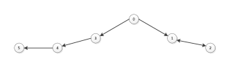
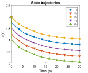
Refer to caption
Figure 1: Communication topology: A network containing five agents.
Refer to caption
Figure 2: State trajectories for the five agents for the one-dimensional example. The dotted lines show the desired state trajectories.

For each agent i,𝑖i, five values of eisubscript𝑒𝑖e_{i}, three values of xisubscript𝑥𝑖x_{i}, and three values of errors corresponding to all the extended neighbors are selected for BE extrapolation, resulting in 5×3si5superscript3subscript𝑠𝑖5\times 3^{s_{i}} total values of isubscript𝑖\mathcal{E}_{i}. All agents estimate the unknown drift parameters using history stacks containing thirty points recorded online using a singular value maximizing algorithm (cf. [49]), and compute the required state derivatives using a fifth order Savitzky-Golay smoothing filter (cf. [50]).
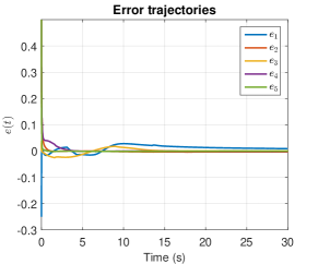
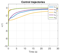
Refer to caption
Figure 3: Tracking error trajectories for the agents for the one-dimensional example.
Refer to caption
Refer to caption
Figure 4: Trajectories of the control input and the relative control error for all agents for the one-dimensional example.
Refer to caption
Refer to caption
Figure 5: Value function weights and drift dynamics parameters estimates for Agent 1 for the one-dimensional example. The dotted lines in the drift parameter plot are the ideal values of the drift parameters.

Figures 2 - 4 show the tracking error, the state trajectories compared with the desired trajectories, and the control inputs for all the agents demonstrating convergence to the desired formation and the desired trajectory. Note that Agents 2, 4, and 5 do not have a communication link to the leader, nor do they know their desired relative position with respect to the leader. The convergence to the desired formation is achieved via cooperative control based on decentralized objectives. Figure 5 shows the evolution and convergence of the value function weights and the parameters estimates for the drift dynamics for Agent 1. The errors between the ideal drift parameters and their respective estimates are large, however, as demonstrated by Figure 3, the resulting dynamics are sufficiently close to the actual dynamics for the developed technique to generate stabilizing policies. It is unclear whether the value function and the policy weights converge to their ideal values. Since an alternative method to solve this problem is not available to the best of the author’s knowledge, a comparison between value function and policy weight estimates and their corresponding ideal values is infeasible.

XI Concluding Remarks

A simulation-based actor-critic-identifier architecture is developed to obtain feedback-Nash equilibrium solutions to a class of differential graphical games. It is established that in a cooperative game based on minimization of the local neighborhood tracking errors, the value function corresponding to an agent depends on information obtained from all their extended neighbors. A set of coupled HJ equations are developed that serve as necessary and sufficient conditions for feedback-Nash equilibrium, and closed-form expressions for the feedback-Nash equilibrium policies are developed based on the HJ equations. The fact that the developed technique requires each agent to communicate with all of its extended neighbors motivates the search for a decentralized method to generate feedback-Nash equilibrium policies.

References

  • [1] R. S. Sutton and A. G. Barto, Reinforcement Learning: An Introduction.   Cambridge, MA, USA: MIT Press, 1998.
  • [2] D. Bertsekas, Dynamic Programming and Optimal Control, 3rd ed.   Belmont, MA: Athena Scientific, 2007, vol. 2.
  • [3] K. G. Vamvoudakis and F. L. Lewis, “Online actor-critic algorithm to solve the continuous-time infinite horizon optimal control problem,” Automatica, vol. 46, no. 5, pp. 878–888, 2010.
  • [4] H. Modares, F. L. Lewis, and M.-B. Naghibi-Sistani, “Integral reinforcement learning and experience replay for adaptive optimal control of partially-unknown constrained-input continuous-time systems,” Automatica, vol. 50, no. 1, pp. 193–202, 2014.
  • [5] V. Konda and J. Tsitsiklis, “On actor-critic algorithms,” SIAM J. Control Optim., vol. 42, no. 4, pp. 1143–1166, 2004.
  • [6] H. Zhang, L. Cui, and Y. Luo, “Near-optimal control for nonzero-sum differential games of continuous-time nonlinear systems using single-network adp,” IEEE Trans. Cybern., vol. 43, no. 1, pp. 206–216, 2013.
  • [7] A. Heydari and S. Balakrishnan, “Finite-horizon control-constrained nonlinear optimal control using single network adaptive critics,” IEEE Trans. Neural Netw. Learn. Syst., vol. 24, no. 1, pp. 145–157, 2013.
  • [8] W. Ren and R. W. Beard, Distributed Consensus in Multi-Vehicle Cooperative Control.   New York: Springer-Verlag, 2008.
  • [9] E. Semsar-Kazerooni and K. Khorasani, Team Cooperation in a Network of Multi-Vehicle Unmanned Systems: Synthesis of Consensus Algorithms.   Springer New York, 2013.
  • [10] R. Murray, “Recent research in cooperative control of multivehicle systems,” J. Dyn. Syst. Meas. Control, vol. 129, pp. 571–583, 2007.
  • [11] M. Tidball and E. Altman, “Approximations in dynamic zero-sum games, i,” SIAM J. Control Optim., vol. 34, no. 1, pp. 311–328, Jan. 1996.
  • [12] M. Tidball, O. Pourtallier, and E. Altman, “Approximations in dynamic zero-sum games, ii,” SIAM J. Control Optim., vol. 35, no. 6, pp. 2101–2117, 1997.
  • [13] R. Isaacs, Differential Games: A Mathematical Theory with Applications to Warfare and Pursuit, Control and Optimization, ser. Dover Books on Mathematics.   Dover Publications, 1999.
  • [14] T. Basar and G. J. Olsder, Dynamic Noncooperative Game Theory: Second Edition, ser. Classics in Applied Mathematics.   SIAM, 1999.
  • [15] E. Altman, O. Pourtallier, A. Haurie, and F. Moresino, “Approximating nash equilibria in nonzero-sum games,” Int. Game Theory Rev., vol. 2, no. 2–3, pp. 155–172, 2000.
  • [16] S. Tijs, Introduction to Game Theory.   Hindustan Book Agency, 2003.
  • [17] J. Nash, “Non-cooperative games,” Annals of Math., vol. 2, pp. 286–295, 1951.
  • [18] K. G. Vamvoudakis and F. L. Lewis, “Online neural network solution of nonlinear two-player zero-sum games using synchronous policy iteration,” in Proc. IEEE Conf. Decis. Control, 2010.
  • [19] D. Vrabie and F. L. Lewis, “Integral reinforcement learning for online computation of feedback nash strategies of nonzero-sum differential games,” in Proc. IEEE Conf. Decis. Control, 2010, pp. 3066–3071.
  • [20] M. Johnson, S. Bhasin, and W. E. Dixon, “Nonlinear two-player zero-sum game approximate solution using a policy iteration algorithm,” in Proc. IEEE Conf. Decis. Control, 2011, pp. 142–147.
  • [21] K. G. Vamvoudakis and F. L. Lewis, “Multi-player non-zero-sum games: Online adaptive learning solution of coupled hamilton-jacobi equations,” Automatica, vol. 47, pp. 1556–1569, 2011.
  • [22] X. Lin and C. G. Cassandras, “An optimal control approach to the multi-agent persistent monitoring problem in two-dimensional spaces,” IEEE Trans. Autom. Control, vol. 60, no. 6, pp. 1659–1664, June 2015.
  • [23] J. Case, “Toward a theory of many player differential games,” SIAM J. Control, vol. 7, pp. 179–197, 1969.
  • [24] A. Starr and C.-Y. Ho, “Nonzero-sum differential games,” J. Optim. Theory App., vol. 3, no. 3, pp. 184–206, 1969.
  • [25] A. Starr and Ho, “Further properties of nonzero-sum differential games,” J. Optim. Theory App., vol. 4, pp. 207–219, 1969.
  • [26] A. Friedman, Differential games.   Wiley, 1971.
  • [27] A. Bressan and F. S. Priuli, “Infinite horizon noncooperative differential games,” J. Differ. Equ., vol. 227, no. 1, pp. 230 – 257, 2006.
  • [28] A. Bressan, “Noncooperative differential games,” Milan J. Math., vol. 79, no. 2, pp. 357–427, Dec. 2011.
  • [29] K. G. Vamvoudakis, F. L. Lewis, and G. R. Hudas, “Multi-agent differential graphical games: Online adaptive learning solution for synchronization with optimality,” Automatica, vol. 48, no. 8, pp. 1598 – 1611, 2012.
  • [30] J. Wang and M. Xin, “Integrated optimal formation control of multiple unmanned aerial vehicles,” IEEE Trans. Control Syst. Technol., vol. 21, no. 5, pp. 1731–1744, 2013.
  • [31] H. Zhang, T. Feng, G. H. Yang, and H. Liang, “Distributed cooperative optimal control for multiagent systems on directed graphs: An inverse optimal approach,” IEEE Trans. Cybern., vol. 45, no. 7, pp. 1315–1326, July 2015.
  • [32] S. Ghosh and J. W. Lee, “Optimal distributed finite-time consensus on unknown undirected graphs,” IEEE Trans. Control Netw. Syst., vol. 2, no. 4, pp. 323–334, December 2015.
  • [33] W. Lin, “Distributed uav formation control using differential game approach,” Aerosp. Sci. Technol., vol. 35, pp. 54–62, 2014.
  • [34] E. Semsar-Kazerooni and K. Khorasani, “Optimal consensus algorithms for cooperative team of agents subject to partial information,” Automatica, vol. 44, no. 11, pp. 2766 – 2777, 2008.
  • [35] D. H. Shim, H. J. Kim, and S. Sastry, “Decentralized nonlinear model predictive control of multiple flying robots,” in Proc. IEEE Conf. Decis. Control, vol. 4, 2003, pp. 3621–3626.
  • [36] L. Magni and R. Scattolini, “Stabilizing decentralized model predictive control of nonlinear systems,” Automatica, vol. 42, no. 7, pp. 1231 – 1236, 2006.
  • [37] A. Heydari and S. N. Balakrishnan, “An optimal tracking approach to formation control of nonlinear multi-agent systems,” in Proc. AIAA Guid. Navig. Control Conf., 2012.
  • [38] H. Zhang, J. Zhang, G. H. Yang, and Y. Luo, “Leader-based optimal coordination control for the consensus problem of multiagent differential games via fuzzy adaptive dynamic programming,” IEEE Trans. Fuzzy Syst., vol. 23, no. 1, pp. 152–163, February 2015.
  • [39] R. Kamalapurkar, L. Andrews, P. Walters, and W. E. Dixon, “Model-based reinforcement learning for infinite-horizon approximate optimal tracking,” IEEE Trans. Neural Netw. Learn. Syst., to appear.
  • [40] S. Khoo and L. Xie, “Robust finite-time consensus tracking algorithm for multirobot systems,” IEEE/ASME Trans. Mechatron., vol. 14, no. 2, pp. 219–228, 2009.
  • [41] D. Liberzon, Calculus of variations and optimal control theory: a concise introduction.   Princeton University Press, 2012.
  • [42] G. V. Chowdhary and E. N. Johnson, “Theory and flight-test validation of a concurrent-learning adaptive controller,” J. Guid. Control Dynam., vol. 34, no. 2, pp. 592–607, Mar. 2011.
  • [43] R. Kamalapurkar, P. Walters, and W. E. Dixon, “Model-based reinforcement learning for approximate optimal regulation,” Automatica, vol. 64, pp. 94–104, 2016.
  • [44] R. A. Horn and C. R. Johnson, Topics in Matrix Analysis.   Cambridge University Press, 1991.
  • [45] R. Kamalapurkar, H. T. Dinh, P. Walters, and W. E. Dixon, “Approximate optimal cooperative decentralized control for consensus in a topological network of agents with uncertain nonlinear dynamics,” in Proc. Am. Control Conf., Washington, DC, Jun. 2013, pp. 1322–1327.
  • [46] R. Kamalapurkar, H. Dinh, S. Bhasin, and W. E. Dixon, “Approximate optimal trajectory tracking for continuous-time nonlinear systems,” Automatica, vol. 51, pp. 40–48, Jan. 2015.
  • [47] H. K. Khalil, Nonlinear Systems, 3rd ed.   Upper Saddle River, NJ: Prentice Hall, 2002.
  • [48] R. Kamalapurkar, “Model-based reinforcement learning for online approximate optimal control,” Ph.D. dissertation, University of Florida, 2014.
  • [49] G. Chowdhary, T. Yucelen, M. Mühlegg, and E. N. Johnson, “Concurrent learning adaptive control of linear systems with exponentially convergent bounds,” Int. J. Adapt. Control Signal Process., vol. 27, no. 4, pp. 280–301, 2013.
  • [50] A. Savitzky and M. J. E. Golay, “Smoothing and differentiation of data by simplified least squares procedures.” Anal. Chem., vol. 36, no. 8, pp. 1627–1639, 1964.
[Uncaptioned image] Rushikesh Kamalapurkar received his M.S. and his Ph.D. degree in 2011 and 2014, respectively, from the Mechanical and Aerospace Engineering Department at the University of Florida. After working for a year as a postdoctoral research fellow with Dr. Warren E. Dixon, he was selected as the 2015-16 MAE postdoctoral teaching fellow. In 2016 he joined the School of Mechanical and Aerospace Engineering at the Oklahoma State University as an Assistant professor. His primary research interest has been intelligent, learning-based control of uncertain nonlinear dynamical systems. His work has been recognized by the 2015 University of Florida Department of Mechanical and Aerospace Engineering Best Dissertation Award, and the 2014 University of Florida Department of Mechanical and Aerospace Engineering Outstanding Graduate Research Award.
[Uncaptioned image] Justin R. Klotz received the Ph.D. degree in mechanical engineering from the University of Florida, Gainesville, FL, USA, in 2015, where he was awarded the Science, Mathematics and Research for Transformation (SMART) Scholarship, sponsored by the Department of Defense. His research interests include the development of Lyapunov-based techniques for reinforcement learning-based control, switching control methods, delay-affected control, and trust-based cooperative control.
[Uncaptioned image] Patrick Walters received the Ph.D. degree in mechanical engineering from the University of Florida, Gainesville, FL, USA, in 2015. His research interests include reinforcement learning-based feedback control, approximate dynamic programming, and robust control of uncertain nonlinear systems with a focus on the application of underwater vehicles.
[Uncaptioned image] Prof. Warren E. Dixon received his Ph.D. in 2000 from the Department of Electrical and Computer Engineering from Clemson University. He was selected as a Eugene P. Wigner Fellow at Oak Ridge National Laboratory (ORNL). In 2004, he joined the University of Florida in the Mechanical and Aerospace Engineering Department. His main research interest has been the development and application of Lyapunov-based control techniques for uncertain nonlinear systems. He has published 3 books, over a dozen chapters, and approximately 125 journal and 230 conference papers. His work has been recognized by the 2015 & 2009 American Automatic Control Council (AACC) O. Hugo Schuck (Best Paper) Award, the 2013 Fred Ellersick Award for Best Overall MILCOM Paper, a 2012-2013 University of Florida College of Engineering Doctoral Dissertation Mentoring Award, the 2011 American Society of Mechanical Engineers (ASME) Dynamics Systems and Control Division Outstanding Young Investigator Award, the 2006 IEEE Robotics and Automation Society (RAS) Early Academic Career Award, an NSF CAREER Award, the 2004 Department of Energy Outstanding Mentor Award, and the 2001 ORNL Early Career Award for Engineering Achievement. He is a Fellow of ASME and IEEE and is an IEEE Control Systems Society (CSS) Distinguished Lecturer. He has served as the Director of Operations for the Executive Committee of the IEEE CSS Board of Governors and as a member of the U.S. Air Force Science Advisory Board. He is currently or formerly an associate editor for ASME Journal of Journal of Dynamic Systems, Measurement and Control, Automatica, IEEE Control Systems Magazine, IEEE Transactions on Systems Man and Cybernetics: Part B Cybernetics, and the International Journal of Robust and Nonlinear Control.