Analysis of Low Excitation HDO Transitions Toward the High-Mass Star-forming Regions G34.26+0.15, W51e₁/e₂, and W49N

Abstract

We present observations of the ground state 1_0,1–0_0,0 rotational transition of HDO at 464.925 GHz and the 1_1,0–1_0,1 transition at 509.292 GHz towards the three high-mass star forming regions: G34.26+0.15, W49N and W51e₁/e₂, carried out with the Caltech Submillimeter Observatory. The latter transition is observed for the first time from the ground. The spectra are modeled, together with observations of higher-energy HDO transitions, as well as submillimeter dust continuum fluxes from the literature, using a spherically symmetric radiative transfer model to derive the radial distribution of the HDO abundance in the target sources. The abundance profile is divided into an inner hot core region, with kinetic temperatures higher than 100 K and a cold outer envelope with lower kinetic temperatures. The derived HDO abundance with respect to H₂ is (0.3–3.7)$\times 10^{-8}$ in the hot inner region ($T>100\mathrm{K}$) and (7.0–10.0)$\times 10^{-11}$ in the cold outer envelope. We also used two H${}_{2}^{18}$O fundamental transitions to constrain the H₂O abundances in the outer envelopes. The HDO/H₂O ratios in these cold regions are found to be (1.8–3.1)$\times 10^{-3}$ and are consequently higher than in the hot inner regions of these sources.

1 Introduction

During the cold phase preceding the formation of stellar objects, molecules freeze-out onto dust grains, forming H₂O- dominated ice mantles, mixed with other less-abundant species. The low temperature and the disappearance of most molecules, especially CO, from the gas phase trigger a peculiar chemistry leading to high abundances of deuterated species. Molecules tend to attach a D atom rather than an H atom, because deuterated species have larger reduced masses and consequently lower binding energies, arising from lower zero-point vibrational energies. Ion-molecule reactions in the gas phase (Brown & Millar, 1989) and reactions on the grain surfaces (Tielens, 1983) are the two possible mechanisms responsible for deuterium enrichments in heavy molecules. The reactions involved are exothermic, which is why significant deuteration levels can be expected in the cold ISM. In the warmer phase, only very little fractionation is expected to occur, because the energy barrier could be overcome by the elevated temperature. However, at the temperatures deduced for the hot core regions (100–200 K) the ice mantles evaporate and the gas again becomes enriched in deuterated species, with abundances elevated compared to the cosmic D/H ratio for a short period, before the chemistry reaches steady-state. These enhancements in the hot cores reflect, to some degree, the grain mantle composition in the earlier, colder cloud phases. Although the processes leading to the water deuteration are not fully understood, they are clearly related to the grain-surface chemistry and the observed HDO/H₂O ratio reveals the chemical and physical history of the protostellar materials (Cazaux et al., 2011; Codella et al., 2010). A recent review of water chemistry can be found in van Dishoeck et al. (2013) and a review of the latest observational results from Herschel.

Early studies of water deuterium fractionation in high-mass hot cores were performed almost twenty years ago, when the submillimeter spectrum was largely inaccessible (Jacq et al., 1990; Schulz et al., 1991; Gensheimer et al., 1996; Helmich et al., 1996). The HDO abundance has been recently determined toward the high-mass hot core G34.26+0.15 and the intermediate-mass protostar NGC7129 FIRS2 (Fuente et al., 2012; Liu et al., 2013; Coutens et al., 2014). Here, we present the new observations of the ground state rotational transition of HDO at 464.925 GHz and the first excited transition at 509.292 GHz toward three high-mass star forming regions: G34.26+0.15, W51e₁/e₂ and W49N. The combination of data taken with the same telescope of both the ground state transition (1_0,1–0_0,0) and the first excited line (1_1,0–1_0,1) provide better constraints on the source structure. These HDO transitions are studied for the first time to probe the structure of the envelope of the W51e₁/e₂ and W49N hot cores. In this paper, we aim at determining the HDO fractional abundances relative to H₂ in the inner and outer region of the core in our target sources using, the static radiative transfer code of Zmuidzinas et al. (1995). We also used two H${}_{2}^{18}$O fundamental transitions observed by Flagey et al. (2013) to constrain the H₂O abundance and the HDO/H₂O ratio in the outer envelopes.

2 Observations

Water is difficult to study from the ground, due to its strong presence in the Earth’s atmosphere. However, many HDO lines, including the ground state 1_0,1–0_0,0 rotational transition and the 1_1,0–1_0,1 excited transition studied here, lie in atmospheric windows, where observations are possible from high sites, under good weather conditions. Table 1 lists the HDO transitions included in the present study and the H${}_{2}^{18}$O transitions which we use to constrain the HDO/H₂O ratio in the outer envelope.

Table 1: Observed and modeled HDO and H${}_{2}^{18}$O rotational transitions.

Species	Transition	Frequency	$E_{\mathrm{up}}$	$A_{\mathrm{ul}}$	Telescope	FWHM
		(GHz)	(K)	(s-1)		(″)
HDO	10,1–00,0	464.925	22.3	$1.69\times 10^{-4}$	CSO	15.7
	11,0–10,1	509.292	47.0	$2.30\times 10^{-3}$	CSO	15.7
	21,1–21,2	241.562	95.2	$1.18\times 10^{-5}$	IRAM	12.0
	31,2–22,1	225.897	167.6	$1.31\times 10^{-5}$	IRAM	13.0
	42,2–42,3	143.727	319.2	$2.80\times 10^{-6}$	IRAM	17.0
	52,3–43,2	255.050	437.2	$1.78\times 10^{-5}$	IRAM	12.0
p-H${}_{2}^{18}$O	11,1–00,0	1101.698	53.9	$1.79\times 10^{-2}$	HIFI	19.2
o-H${}_{2}^{18}$O	21,2–10,1	1655.868	114.0	$1.26\times 10^{-2}$	HIFI	12.8

2.1 Source description

The 1_0,1–0_0,0 ground-state rotational transition of HDO at 465 GHz and the 1_1,0–1_0,1 transition at 509 GHz were observed toward three high-mass star forming regions are listed in Table 2. All the sources are characterized by strong millimeter continuum and mid-infrared emission, characteristic of the early stage of high-mass star formation.

G34.26+0.15 is one of the best studied high-mass star-forming regions in the Milky Way. Embedded within this molecular cloud is a hot core, which exhibits strong H₂O maser emission and high abundances of saturated molecules (MacDonald et al., 1996); two unresolved UCHII regions, labeled A and B; a more evolved H II region with a cometary shape; and an extended, ring-like H II region (Reid & Ho, 1985). Based on narrow-band mid-infrared imaging of the complex, Campbell et al. (2000) concluded that the same star is responsible for ionization of the cometary H II component (C) and heating the dust, but is not interacting with the hot core seen in the molecular emission. At a 12″ resolution, Hunter et al. (1998) also found the peak of the 350 $\mu$m emission to coincide with the component C of the UCHII region.

The radio continuum emission of W51 shows three separate components: W51 IRS1, W51 IRS2, and W51 Main. W51 Main is defined by a group of OH and H₂O masers near several UCHII regions. The continuum emission from ultracompact H II regions was resolved into compact components labeled W51e₁ to W51e₈ (Zhang & Ho, 1997). Of these, e₁ and e₂ are the brightest in high-resolution continuum maps.

The star forming region W49N contains at least a dozen UCHII regions powered by OB-type stars arranged in a ring 2 pc in diameter (De Pree et al., 2000). Evidence that star formation is still in progress within W49N comes from strong H₂O maser emission and strong millimeter continuum emission attributed to dust condensations (Sievers et al., 1991).

Table 2: Source sample.

Source	$\alpha$(J2000)	$\delta$(J2000)	$D$
			(kpc)
G34.26+0.15	18 53 18.6	+01 14 57.7	3.8
W51e1/e2	19 23 43.9	+14 30 25.9	5.4
W49N	19 10 13.2	+09 06 12.0	11.4

2.2 Observations

Observations of the 465 GHz and 509 GHz HDO transitions presented here were carried out in 2012 June–August, using the 10.4 m Leighton Telescope of the Caltech Submillimeter Observatory (CSO) on Mauna Kea, Hawaii. We used the new wideband 460 GHz facility SIS receiver and the FFTS backend that covers the full 4 GHz intermediate frequency (IF) range with a 270 kHz channel spacing. Pointing of the telescope was checked by performing five-point continuum scans of planets and strong dust continuum sources. The spectra were obtained in antenna temperature units $T^{*}_{A}$, and then converted to the main beam brightness temperature, $T_{\mathrm{mb}}$, via the relation $T^{*}_{A}$ = $\eta_{\mathrm{mb}}$$T_{\mathrm{mb}}$, $\eta_{\mathrm{mb}}$ is the CSO main-beam efficiency, which is found to be $\sim 37\%$ at 460 GHz from total power observations of planets. The absolute calibration uncertainty of the individual measurements is $\sim$20%.

In addition to the new CSO data, we included in our analysis previously published observations of higher-energy transitions (Jacq et al., 1990) toward our target sources. We used the reduced HIFI data of the H${}_{2}^{18}$O transitions at 1101.698 and 1655.868 GHz. The HDO and H${}_{2}^{18}$O lines parameters are listed in Table 3. The H${}_{2}^{18}$O ground state transitions have been previously presented by Flagey et al. (2013).

The data processing was done using the IRAM GILDAS software package (Pety, 2005). We measured the line parameters: central velocity $V_{LSR}$, the full-width at half maximum (FWHM) $\Delta{V}$, peak intensity $T^{peak}$, by fitting a single gaussian profile to the data (in $T_{\mathrm{mb}}$ units). The integrated line intensity is equal to $W_{i}$ = $\int{T_{i}}dV$, where $i$ either refers to observations (obs) or models (mod).

We also used Herschel/HIFI data at 893 GHz (Vastel et al. in preparation) obtained by the PRISMAS guaranteed time key program, and the SCUBA data at 353 GHz that provide an accurate determination of the source continuum flux.
The PRISMAS continuum observations were obtained in the double beam switching mode. At 800 GHz, the HIFI beam size is 26.5 $\arcsec$ and the instrument gain is 469 Jy/K (Roelfsema et al., 2012).

Table 3: HDO and H${}_{2}^{18}$O lines parameters.

Source	Species	Frequency	$V_{\mathrm{LSR}}$	$\triangle V$	$T^{peak}_{obs}$	$W_{obs}$	$W_{mod}$
		(GHz)	(km s-1)	(km s-1)	(K)	(K km s-1)	(K km s-1)
G34.26	HDO
		143	57.7 (0.2)	6.9 (0.4)	0.4	2.6 (0.2)	1.7
		225	57.4 (0.3)	6.6 (0.4)	1.2	8.4(0.7)	11.4
		241	57.7 (0.3)	7.0 (0.6)	1.8	13.2(1.0)	12.0
		255	57.7 (0.9)	8.8 (3.0)	0.6	6.0 (0.6)	3.4
		465	58.0 (0.1)	6.4 (0.2)	1.8	12.1(0.3)	13.2
		509	58.4 (0.2)	6.0 (0.7)	0.8	5.5 (0.8)	10.4
	H${}_{2}^{18}$O
		1102	61.1 (0.1)	3.5 (0.2)	-0.9	-3.4(0.2)	-2.6
		1656	61.1 (0.2)	6.5(0.0)	-1.7	-11.7 (0.9)	-13.5
W51e1/e2	HDO
		225	55.0 (0.4)	9.2 (0.9)	0.6	6.2(0.6)	4.5
		241	55.6 (1.6)	5.7 (1.6)	0.8	4.7(1.1)	5.5
		255	53.9 (2.0)	15.6 (6.0)	0.3	5.6(2.0)	2.1
		465	57.1 (0.2)	6.4 (0.4)	1.3	8.7(0.4)	10.7
		509			$<$ 0.9	$<$ 3.5	4.1
	H${}_{2}^{18}$O
		1102	58.3 (0.1)	6.1 (0.3)	-0.9	-5.8(0.3)	-5.7
		1656	58.7 (0.1)	8.3(0.3)	-2.1	-18.3 (0.6)	-20.0
W49N	HDO
		465	8.5(0.2)	12.0 (0.5)	0.8	10.8 (0.4)	9.4
		509	8.1 (0.7)	12.9 (1.5)	0.7	10.2 (1.2)	8.9
	H${}_{2}^{18}$O
		1102	10.3 (0.2)	9.6 (0.4)	-0.7	-7.5(0.3)	-7.7
		1656	10.4 (0.1)	12.0(0.1)	-2.3	-30.2 (0.3)	-26.4

3 Determination of the HDO and H₂O Abundance

3.1 Modeling

The goal of this study is to determine the HDO fractional abundance in three high-mass stars formation regions. To reproduce the observed line intensities (Table 3) the static radiative transfer code of Zmuidzinas et al. (1995) is used. The model cloud is divided into 200 radial shells, and the code uses a multilevel accelerated lambda-iteration method (Rybicki & Hummer, 1991) to solve for the HDO level populations and the line and continuum radiative transfer in a self-consistent fashion. This radiative transfer program takes into account the excitation of HDO molecules by collisions, line radiation, and dust continuum radiation at the HDO line frequencies. However, IR radiative pumping through HDO vibrationally excited levels and the large-scale velocity field, characteristic of infall or expansion, are not included. The HDO collisional rates used in this study were recently computed by Faure et al. (2012) and Wiesenfeld et al. (2011) for ortho-H₂ and para-H₂ in the temperature range 5–300 K and for all rotational transitions with an upper energies less than 444 K. In the modelling, we assumed a constant ortho-to-para ratio (OPR) of H₂ equal to 3. The ortho and para H₂O collisional rates with ortho and para H₂ were taken from the LAMDA data base (Schröier et al., 2005; Daniel et al., 2011). These rates were calculated for temperatures in the range from 5 to 1500 K including energy levels up to 2000 K above ground. The same collisional rates are used for the H${}_{2}^{18}$O isotopologue. The limitation imposed by the radiative transfer code is to use a single collisional partner in the calculations. We assume that all hydrogen is in the ortho state.

We carried out model calculations from the inner core radius, $r_{min}$, to the outer radius, $r_{max}$ (with ${r_{max}}/{r_{min}}\sim 100$ for all sources; Hatchell & van der Tak 2003). The distance of the edge of the core from the star is set at $r_{min}\sim 2.0\times 10^{16}$ cm or $\sim 1000$ AU, with no dust emission seen at the smaller radii. The lack of submillimeter emission in the core centers could be due to optical depth effects or a central cavity (van der Tak et al., 2000). We adopted a dust-to-gas ratio of 1:100 and a power-law H₂ density distribution of the form:

$$n(r)=n_{0}\bigg{(}\frac{r}{r_{min}}\bigg{)}^{-1.5}\qquad$$ (1)

where $n_{0}$ is the H₂ density at the reference radius ($r_{min}=1000$ au). The power-law index was set to 1.5 in accordance with the static infall theory in the inner part of the object (Shu, 1977; van der Tak et al., 2000; Beuther et al., 2002; Marseille et al., 2010). We assumed that the gas and dust radial temperature profiles follow a power law (Viti & Williams, 1999):

$$T(r)=T_{0}\bigg{(}\frac{r}{r_{min}}\bigg{)}^{-0.5}$$ (2)

where $T_{0}$ represents the maximum temperature of dust grains. We assumed that, at densities found in the hot cores, the gas temperature is equal to the dust temperature.

3.2 Dust emissivity index $\beta$

When molecules deplete inside prestellar cores, dust emission may represent the best tracer of the gas density distribution just prior to the onset of gravitational collapse. The dust continuum optical depth is described by a power-law frequency dependence, $\tau\propto\nu^{\beta}$, and to fit the observed spectral energy distribution, the knowledge of the grain emissivity spectral index, $\beta$, is required. The dust emissivity index depends on the dust grain composition, size, and temperature (Hildebrand, 1983; Goldsmith et al., 1997). Details of the dust-modelling process can be found in the reviews by Draine (2003). Observationally, there have been many attempts at determining and explaining $\beta$. Typical values of $\beta$ range between 1 and 2, with further support for $\beta$ = 1.5–2.0 coming from observations: Wright et al. (1992), Minier et al. (2005) and Gordon et al. (2010). Planck Collaboration XIV (2013) used Planck HFI data with ancillary radio data to study the emissivity index. They computed a median value of far infrared spectral index $\beta_{FIR}$ = $1.88~{}\pm~{}0.08$ at the high frequency Planck channels ($\nu\geq 353$ GHz) and a median value of spectral index $\beta_{mm}$ = $1.6~{}\pm~{}0.06$ at millimeter wavelengths ($\nu<353$ GHz). We can estimate the dust grain emissivity exponent from observations at two frequencies $\nu_{1}$ and $\nu_{2}$ (Hill et al., 2006):

$$\beta=\frac{{\log\frac{F_{\nu_{2}}}{F_{\nu_{1}}}}+\log\frac{({\rm e}^{h\nu_{2}/kT_{\mathrm{dust}}}-1)}{({\rm e}^{h\nu_{1}/kT_{\mathrm{dust}}}-1)}}{{\log\frac{\nu_{2}}{\nu_{1}}}}-3$$ (3)

where $F_{\nu}$ is the source flux density, $\nu$ the frequency of the observations, and $T_{\mathrm{dust}}$ the dust temperature. In this work, the dust grain emissivity index $\beta$ is determined for G34.26 using the millimeter ($\lambda_{1}$ = 1.2 mm; $\nu_{1}$ = 250 GHz) data obtained with SIMBA and submillimeter ($\lambda_{2}$ = 450 $\mu$m; $\nu_{2}$ = 660 GHz) SCUBA data. We derive $\beta=1.6\pm 0.48$. The uncertainty in $\beta$ is typically 30% for the 20–50 K temperature range (Hill et al., 2006). The spectral index for the other sources is taken from literature: Ward-Thompson & Robson (1990) for W49N and from Gordon & Jewell (1987) for W51. The HDO lines studied here are seen in emission, and the model intensities are not sensitive to the exact value of $\beta$, especially for $T>30~{}\mathrm{K}$. That is why the dust grain emissivity index is fixed, and not a free parameter, in the fits.

The values of $\beta$ in our target sources, as well as the continuum fluxes from SCUBA and Herschel/HIFI observations, are listed in Table 4. These are used to constrain the density and temperature distributions as input to the line modeling.

3.3 Modeling procedure

We approximated the radial variation of the HDO fractional abundance, $X=n(HDO)/n(H_{2})$ as a step function with an enhanced abundance $X_{in}$ in the inner region where $T\geq 100~{}\mathrm{K}$, and a lower value $X_{out}$ for the outer envelope where $T<100~{}\mathrm{K}$. Laboratory studies indicate that the evaporation temperature lies in the 90–110 K range, depending on the ice composition and structure (Fraser et al., 2005). In this work the sublimation temperature of water, $T=100$ K (Fraser et al., 2001), is applied as the jump temperature. The model uses the following free parameters: $n_{0}$, $T_{0}$ and $X_{in}$ (for $T\geq 100~{}\mathrm{K}$) and $X_{out}$ (for $T<100~{}\mathrm{K}$). We determine the continuum flux density per beam at 353 GHz (850 $\mu$m), 509 GHz (590 $\mu$m), and 893 GHz (336 $\mu$m) from the model.

Table 4: Continuum flux densities and grain emissivity exponents

Source	$F_{353}$	$F_{509}$	$F_{893}$	$\beta$
	(Jy/beam)	(Jy/beam)	(Jy/beam)
G34.26 + 0.15	56.1	310	1320	1.6
W51e1/e2		400	1490	1.7
W49N		320	1450	1.8

Finally, the synthetic spectra and continuum emission are convolved to the appropriate telescope beam size for comparison with the observations. We minimize the ‘figure of merit’ (FOM) with the method of Jacq et al. (1990) to find the best model of the source. The FOM is computed from the observed and modeled spectra and continuum fluxes according to the following formula:

$$FOM=FOM_{1}+FOM_{2}=\sum_{n}\frac{(T_{\mathrm{obs}}-T_{\mathrm{mod}})^{2}}{(T_{\mathrm{obs}})^{2}}+\sum_{m}\frac{(F_{\mathrm{obs}}-F_{\mathrm{mod}})^{2}}{(F_{\mathrm{obs}})^{2}}$$ (4)

for a set of $n$ spectral lines and $m$ continuum flux densities. The inner and outer HDO abundances are constrained by the spectral line data ($FOM_{1}$), whereas model parameters describing the density and temperature distribution are constrained primarily by the continuum SED ($FOM_{2}$). To determine the uncertainty of $X_{in}$ and $X_{out}$, we performed $\chi^{2}$ analysis. In analogy to Lampton method (Lampton et al., 1976) we define $S$ $\equiv$ $FOM_{1}/\sigma^{2}$ $=$ $\sum_{n}\frac{(T_{\mathrm{obs}}-T_{\mathrm{mod}})^{2}}{(\sigma T_{\mathrm{obs}})^{2}}$, where $n$ being the number of spectral lines. The $\sigma$ within analysis $\chi^{2}$ includes a calibrations uncertainty of $20\%$ for all individual measurments. The difference, $\Delta{S}$ $\equiv$ $S_{true}-S_{min}$ is distributed as $\chi^{2}$ with $p$ degrees of freedom (here: $p$=2; $X_{in}$ and $X_{out}$). By $\Delta{S}$ $\sim$ $\chi^{2}_{p}$  ($"\sim"$ - ”is distributed as”) we mean for any number L probability: $Prob~{}(\Delta{S}>L)$ = $Prob~{}(\chi^{2}_{p}>L)$ . With the limiting contour value $S_{L}$ defined as $S_{min}+L$, $Prob~{}(\Delta{S}>S_{L}-S_{min})$ = $Prob~{}(S_{true}>S_{L})$ = $Prob~{}(\chi^{2}_{p}>S_{L}-S_{min})$. $Prob~{}(S_{true}>S_{L})$ is the probality $\alpha$ of the contour failing to enclose the true value, hence $\alpha$ = $Prob~{}(\chi^{2}_{p}>S_{L}-S_{min})$. The $\alpha$-point of $\chi^{2}$ distribution is defined by $\alpha$ $\equiv$ $Prob~{}[\chi^{2}_{p}>\chi^{2}_{p}(\alpha)]$. Significance $\alpha$ is $S_{L}$ = $S_{min}+\chi^{2}_{p}(\alpha)$. In this expression, $\chi^{2}_{p}(\alpha)$ is tabulated value of $\chi^{2}$ distribtion for $p$ degrees of freedom and significance $\alpha$. Equivalently, any one observation’s contour has a confidence $C=1-\alpha$ of enclosing the true parameter vector. The required contours for significance are 1$\sigma$, 2$\sigma$, and 3$\sigma$, which respectively represent a confidence of 68.3$\%$, 95.4$\%$, and 99.7 $\%$ of enclosing the true value of $X_{in}$ and $X_{out}$. The contours correspond to $S_{L}=S_{min}+2.17$, $S_{L}=S_{min}+6.17$, and $S_{L}=S_{min}+11.8$.
We used models with the same physical parameters as those used for HDO in the analysis of the H${}_{2}^{18}$O data. The two H${}_{2}^{18}$O fundamental transitions were modeled independently and the resulting ortho/para ratio of water is consistent with the high temperature value of given the modeling uncertainties .

3.4 Results

3.4.1 Origin of The Lines

Figure 1 shows fractional population of the HDO levels of the relevant features of our dataset calculated in our model. The high-energy transitions are sensitive to changes in $X_{in}$. Indeed the bulk of emission in the high energy transitions is produced in the inner

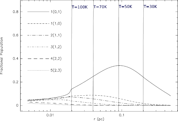
Figure 1: Fractional population of the HDO energy levels as a function of the radius of the cloud.

hot-core region where $T>100~{}\mathrm{K}$. In the G34.26 source, this region has a radius equal to 1.0″ which corresponds to 0.02 pc. This is in agreement with the interferometric observations of the HDO lines at 225 and 241 GHz by Liu et al. (2013). That is the reason why the high-energy transitions are sensitive to changes in $X_{in}$. On the other hand, the 465 and 509 GHz HDO transitions are sensitive primarily to $X_{out}$. The 509 GHz line arises predominantly in the region between the warm envelope and the cold region ($T\sim$ 50–100 $\mathrm{K}$), whereas the 465 GHz transition is produced in the cold envelope ($T<50~{}\mathrm{K}$). The ground-state rotational transition of HDO at 465 GHz is consequently a very good probe of the abundance in the cold outer envelope, which is consistent with the results of Parise et al. (2005) for the solar-type protostar IRAS 16293-2422. The 509 GHz transition provides particurlarly good constraints on the HDO abundance profile in the transition region between the hot core and the envelope, and should be included in future, more advanced models of HDO in high-mass star-forming regions. The model reproduces the observed intensities of different transitions in our target sources, with the exception of the 509 GHz line in G34.26. Although the signal-to-noise ratio of the observed 509 GHz spectrum is limited, it is clear that the best-fit model does not reproduce this line profile. The 509 GHz transition is formed in the part of the cloud where, within the scenario proposed by Rolffs et al. (2010), various feedback: thermal, radiative, or turbulent mechanisms are expected during the process of massive stars formation. In particular, it should be noted that, with the inclusion of velocity fields in their model, Coutens et al. (2014) succesfully reproduced the 509 GHz line observed with Herschel/HIFI toward this same source. Other possibility is an accretion disk that is fed by the infalling envelope. This is also supported by observations made by Keto et al. (1987) of G34.26. The size of this possible disk is about 9000 au (0.05 pc) (Garay & Rodriguez, 1990; Hajigholi et al., 2016) and agrees well with the place where the 509 GHz line arises (see Figure 1). This model of the G34.26 source (Hajigholi et al., 2016) neither confirm or refute the presence of an expansion in the inner parts of the envelope (Coutens et al., 2014). We concluded that the geometry and physical structure of our model is too simplistic, and that is why we could not to reproduce the 509 GHz line.

3.4.2 Target sources

G34.26+0.15: Observed spectra (black line) and gaussian fit (blue line) of the 465 and 509 GHz HDO transitions toward G34.26+0.15 along with the best-fit model (red line) are shown in Figure 2.

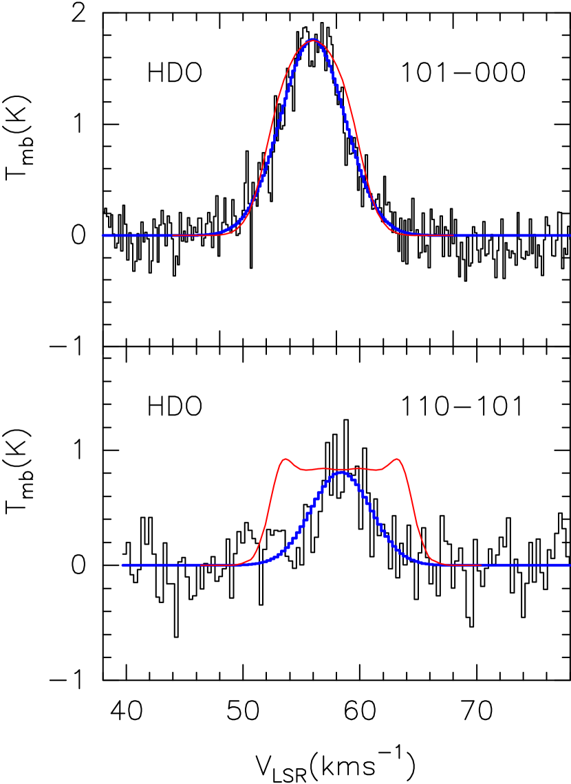
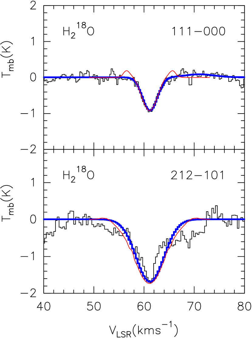
Figure 2: Observed spectra of the 465 and 509 GHz HDO lines and 1102 and 1656 GHz H${}_{2}^{18}$O lines towards G34.26+0.15. The Gaussian fits are shown in blue, while the best-fit model in red.

Model results are presented in Table 5. We obtain the best–fit model for: $T_{0}=200$ K, $n_{0}=1.0\times 10^{8}\,cm^{-3}$,  $X_{in}=3.7\times 10^{-8}$ and $X_{out}=7.8\times 10^{-11}$. We calculated continuum flux densities at 353, 509, and 893 GHz. The resulting uncertainties of $X_{in}$ and $X_{out}$ are shown in Figure 3 and listed in Table 8.

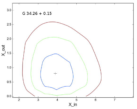
Figure 3: $X_{in}$ and $X_{out}$ HDO abundance contours at 1$\sigma$, 2$\sigma$, 3$\sigma$ for $\chi^{2}$. The best-fit model is represented by the symbol $"+"$ ($X_{in}$ = a$\times 10^{-8}$, $X_{out}$ = b$\times 10^{-10}$).

Observed and modeled spectra of the para-H${}_{2}^{18}$O line at 1102 GHz and the ortho-H${}_{2}^{18}$O line at 1656 GHz are shown in Figure 2. The derived OPR in G34.26 is 1.9. The total (ortho+para) H${}_{2}^{18}$O abundance in the envelope $X_{out}$, is 4.9$\times 10^{-11}$. The recommended isotopic abundance ratio between ¹⁶O and ¹⁸O is 500 (Lodders, 2003). Using this value, the H₂O outer abundance is 2.5$\times 10^{-8}$ and the outer HDO/H₂O ratio is 3.1$\times 10^{-3}$ in the envelope. Considering the results with a 20$\%$ calibration uncertaint, the outer abundance ratio is (2.5 - 3.7)$\times 10^{-3}$.

Table 5: Line intensities and continuum fluxes for the best fit model of G34.26+0.15.

HDO	Freq	$T_{\mathrm{obs}}$	$T_{\mathrm{mod}}$	$FOM_{1}$
transitions	(GHz)	(K)	(K)
10,1–00,0	464.925	1.8	1.8	0.00
11,0–10,1	509.292	0.8	0.8	0.00
21,1–21,2	241.562	1.8	1.6	0.01
31,2–22,1	225.897	1.2	1.4	0.03
42,2–42,3	143.727	0.4	0.5	0.06
52,3–43,2	255.050	0.6	0.4	0.11
Flux (Jy/beam)	$F_{353}$	$F_{353_{\mathrm{mod}}}$		$FOM_{2}$
	56.1	56.4		0.00
	$F_{509}$	$F_{509_{\mathrm{mod}}}$
	310	376		0.05
	$F_{893}$	$F_{893_{\mathrm{mod}}}$
	1320	1525		0.02
				$FOM$ = 0.28

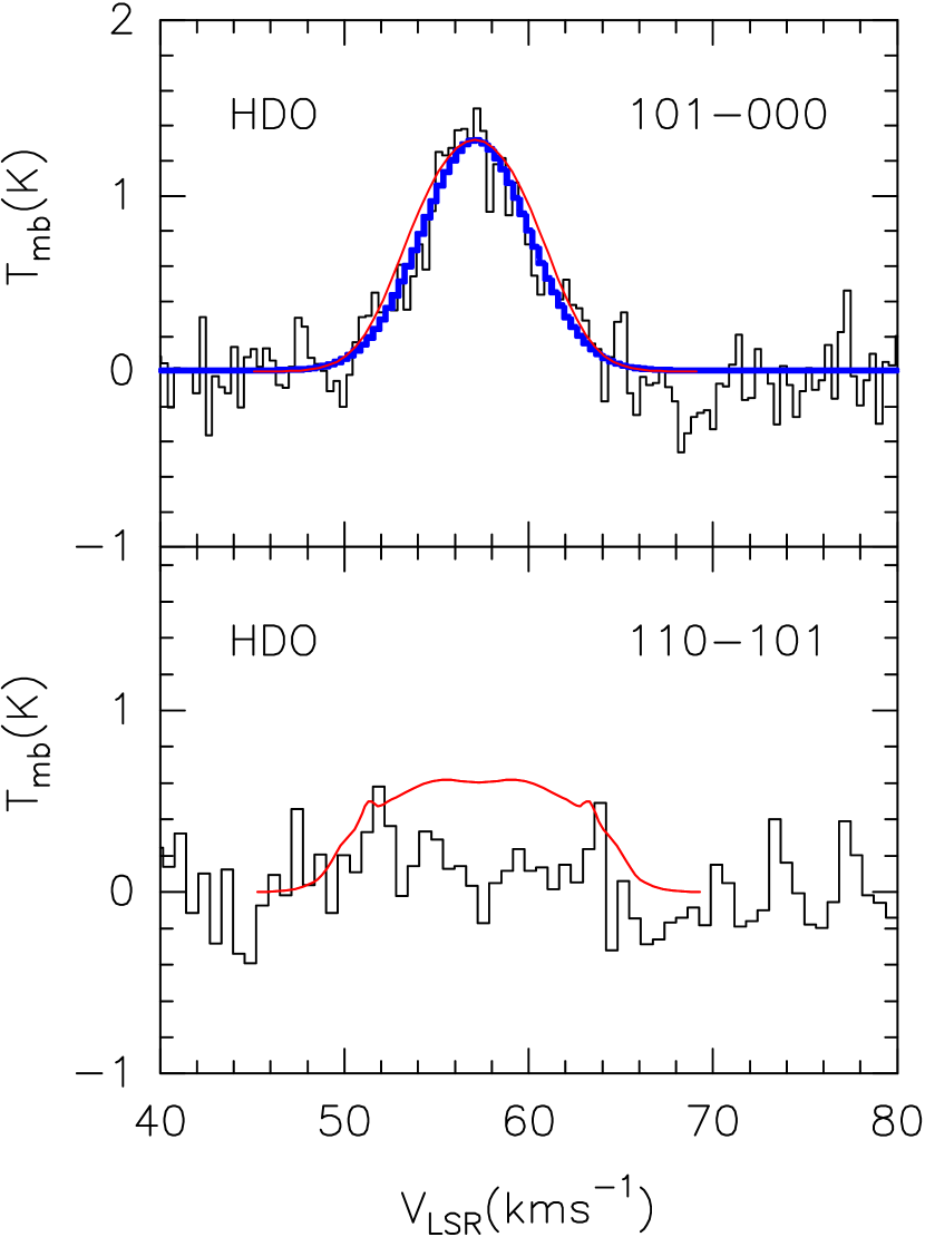
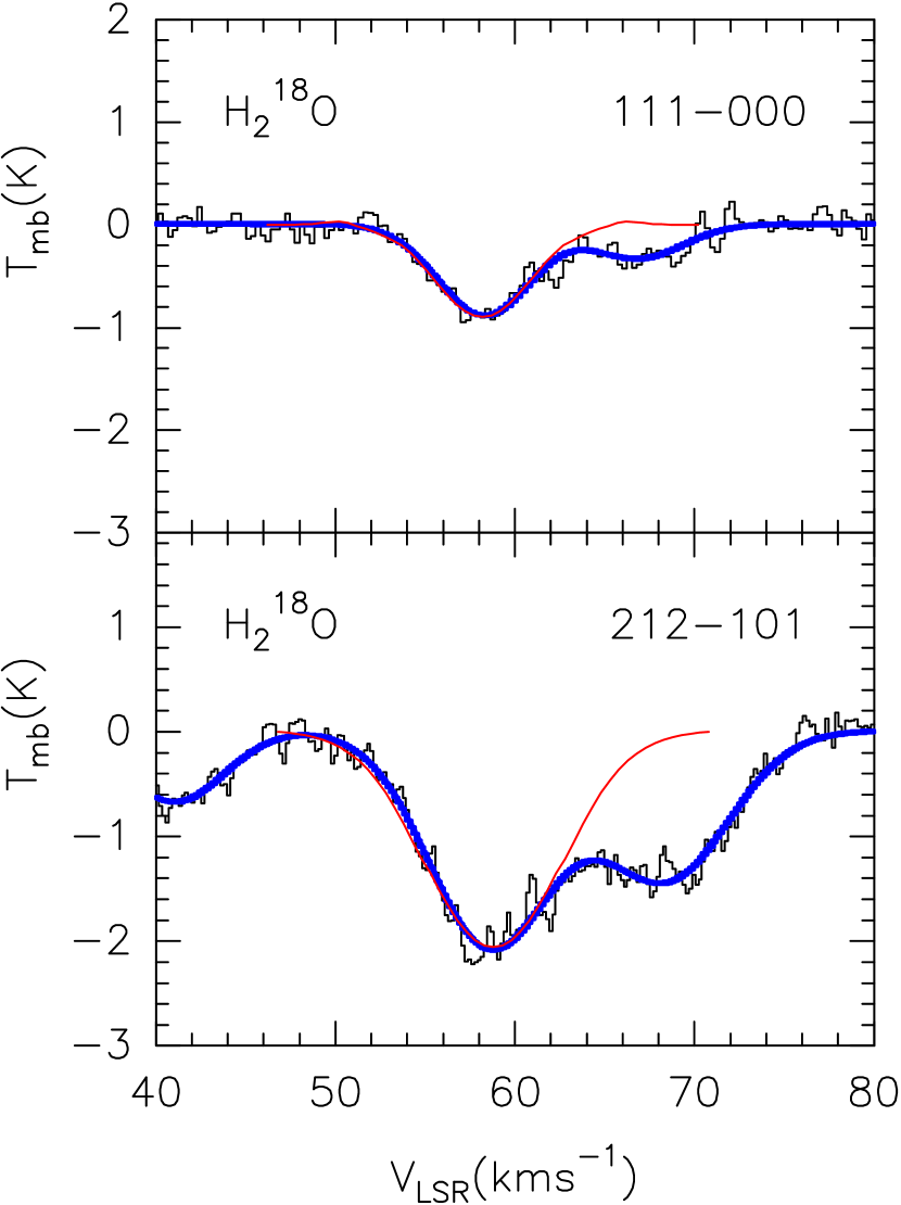
Figure 4: Observed spectra of the 465 and 509 GHz HDO lines and 1102 and 1656 GHz H${}_{2}^{18}$O lines toward W51e₁/e₂.The Gaussian fits are shown in blue, while the best-fit model in red.

W51e₁/e₂: Observed spectra and gaussian fit of the 465 and 509 GHz HDO transitions toward W51e₁/e₂ along with the best-fit model, are shown in Figure 4 by black, blue and red lines, respectively. Model results for W51 are presented in Table 6. We obtain the best fit for: $T_{0}=230~{}\mathrm{K}$, $n_{0}=1.8\times 10^{8}\,cm^{-3}$,  $X_{in}=1.7\times 10^{-8}$ and $X_{out}=7.0\times 10^{-11}$. The resulting uncertainties of $X_{in}$ and $X_{out}$ are shown in Figure 5 and listed in Table 8.
Model flux densities per beam at 509 GHz and 893 GHz for W51 are also listed in Table 6.

Figure 5: $X_{in}$ and $X_{out}$ HDO abundance contours at 1$\sigma$, 2$\sigma$, 3$\sigma$ for $\chi^{2}$. The best-fit model is represented by the symbol $"+"$ ($X_{in}$ = a$\times 10^{-8}$, $X_{out}$ = b$\times 10^{-10}$).

Observed and modeled spectra of the para-H${}_{2}^{18}$O line at 1102 GHz and the ortho-H${}_{2}^{18}$O line at 1656 GHz are shown in Figure 4. The total H${}_{2}^{18}$O abundance (OPR = 2.9) in the envelope $X_{out}$, is $5.5\times 10^{-11}$. The H₂O outer abundance is 2.8$\times 10^{-8}$ and outer HDO/H₂O ratio is 2.5$\times 10^{-3}$. Considering the results with the 20$\%$ calibration uncertainty the outer ratio is (2.0 - 3.0)$\times 10^{-3}$.

Table 6: Line intensities and continuum fluxes for the best fit model of W51e₁/e₂.

HDO	Freq	$T_{\mathrm{obs}}$	$T_{\mathrm{mod}}$	$FOM_{1}$
transitions	(GHz)	(K)	(K)
10,1–00,0	464.925	1.3	1.3	0.00
21,0–10,1	509.292	$<$0.9	0.6
21,1–21,2	241.562	0.8	0.8	0.00
31,2–22,1	225.897	0.6	0.67	0.01
52,3–43,2	255.050	0.3	0.2	0.11
Flux (Jy/beam)	$F_{509}$	$F_{509_{\mathrm{mod}}}$		$FOM_{2}$
	400	350		0.02
	$F_{893}$	$F_{893_{\mathrm{mod}}}$
	1490	1509		0.00
				$FOM$ = 0.14

W49N: Observed spectra and gaussian fit of the 465 and 509 GHz HDO transitions toward W49N along with the best-fit model are shown in Figure 6 by black, blue and red lines, respectively. Model results for W49N are presented in Table 7.We obtain the best fit for: $T_{0}=300~{}\mathrm{K}$, $n_{0}=2.5\times 10^{8}\,cm^{-3}$,  $X_{in}=0.3\times 10^{-8}$ and $X_{out}=10\times 10^{-11}$. The resulting uncertainties of $X_{in}$ and $X_{out}$ are shown in Figure 7 and listed in Table 8.
As data on the high excitation lines are missing for W49N, the inner abundance $X_{in}$ is not as well constrained as in the other sources.

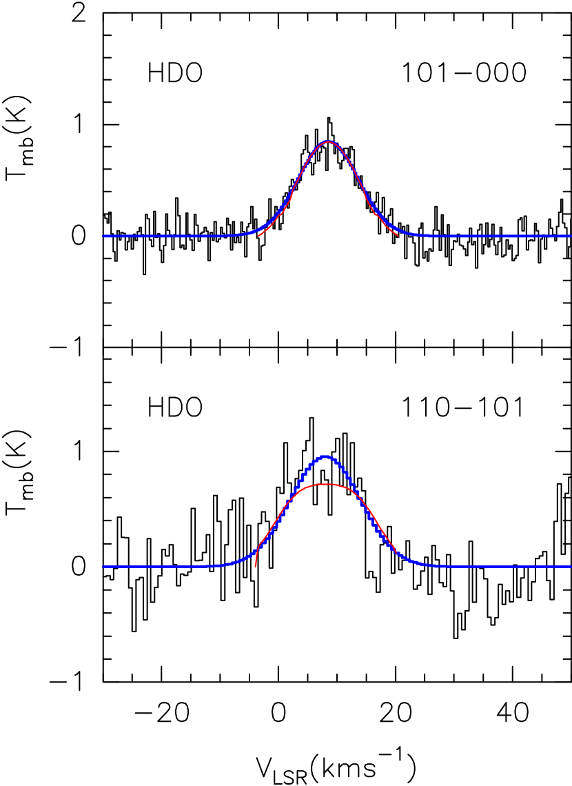
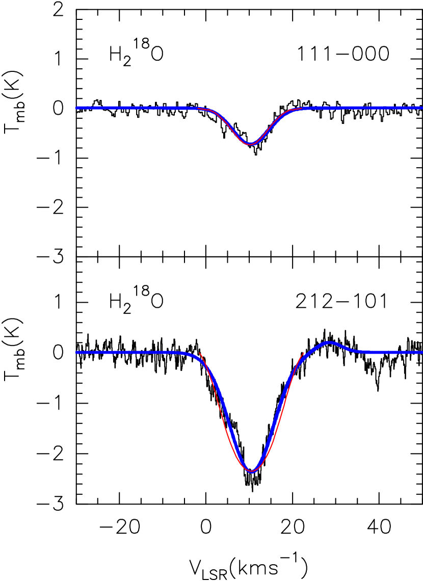
Figure 6: Observed spectra of the 465 and 509 GHz HDO lines and 1102 and 1656 GHz H${}_{2}^{18}$O lines toward W49N. The Gaussian fits are shown in blue, while the best-fit model in red.

Observed and modeled spectra of the para-H${}_{2}^{18}$O line at 1102 GHz and the ortho-H${}_{2}^{18}$O line at 1656 GHz are shown in Figure 6. The total H${}_{2}^{18}$O (OPR = 3.1) abundance in the envelope $X_{out}$, is $1.1\times 10^{-10}$. The H₂O outer abundance is 5.5$\times 10^{-8}$ and the outer HDO/H₂O ratio is 1.8$\times 10^{-3}$. Considering the results with the 20$\%$ calibration uncertainty, the outer abundance ratio is (1.4 - 2.2)$\times 10^{-3}$.

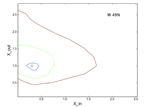
Figure 7: $X_{in}$ and $X_{out}$ HDO abundance contours at 1$\sigma$, 2$\sigma$, 3$\sigma$ for $\chi^{2}$. The best-fit model is represented by the symbol $"+"$ ($X_{in}$ = a$\times 10^{-8}$, $X_{out}$ = b$\times 10^{-10}$).

Table 7: Line intensities and continuum fluxes for the best fit model of W49N.

HDO	Freq	$T_{\mathrm{obs}}$	$T_{\mathrm{mod}}$	$FOM_{1}$
transitions	(GHz)	(K)	(K)
10,1–00,0	464.925	0.8	0.8	0.00
21,0–10,1	509.292	0.7	0.6	0.02
Flux (Jy/beam)	$F_{509}$	$F_{509_{\mathrm{mod}}}$		$FOM_{2}$
	320	310		0.00
	$F_{893}$	$F_{893_{\mathrm{mod}}}$
	1450	1410		0.01
				$FOM$ = 0.03

4 Discussion

4.1 Comparison with Previous Studies

Previous observations of the high-mass star-forming regions indicate an HDO abundance in the hot cores (T $>$ 100 K) but not in the outer, cooler envelopes (T $<$ 100K) (Jacq et al. 1990, Gensheimer et al. 1996, Pardo et al. 2001; see Table 9). We could find variations in the derived HDO abundances in the hot cores between $1.5\times 10^{-9}$ and $2.0\times 10^{-7}$. Jacq et al. (1990) belived that, independent of all modeling, a value much lower than $3.0\times 10^{-8}$ for HDO/H₂ in the hot core is very unlikely. For the first time, Comito et al. (2003, 2010) estimated the HDO abundance in both the inner and outer region of the high-mass source Sgr B2(M). These are, respectively: $3.5\times 10^{-9}$ (T$>$200K), $1.5\times 10^{-9}$ (100 K$<$T$<$200 K) and $2.5\times 10^{-11}$ (T$<$100K). The singly deuterated form of water has been also observed in the massive source AFGL 2591, with abundance varying from $1\times 10^{-7}$ in the hot core and $4\times 10^{-9}$ in the outer envelope (van der Tak et al., 2006). Liu et al. (2013) and Coutens et al. (2014) determined the HDO abundance and HDO/H₂O ratio in the inner and outer region of G34.26 (see Table 9). We derived the HDO abundances of $X_{in}$ and $X_{out}$ in three high-mass star-forming regions: G34.26, W 49N, and W51. We found a difference between our $X_{in}(HDO)$ and $X_{out}(HDO)$ values for G34.26 and those reported by Coutens et al. (2014) and Liu et al. (2013), respectively. This is likely because the first authors used different model structures and a higher jump temperature, and the second authors did not check the higher value of $X_{out}(HDO)$ in their model. The obtained HDO abundances of our target sources in the hot cores and the cooler envelopes are relatively consistent with the values found in the other high-mass star-forming regions (Kulczak-Jastrzȩbska, 2016). These results show that the HDO abundance is enriched in the inner regions of high-mass protostars because of the sublimation of the ice mantles, in the same way as for other studies low- and high-mass sources (e.g. NGC 1333 IRAS2A, IRAS 162923-2422, AFGL 2591, G34.26; Table 9). Observations of sites of high-mass star formation show in general the lower HDO abundances than observations of low-mass star forming cores. Possibly for high-mass protostars, the very cold and dense pre-collapse phase where CO freeze-out onto the grain mantles lasts only a short time, and the chemical reactions leading to the enhancement of deuterium abundance being strongly depressed when the temperature increases (Caselli et al., 2008).

4.2 Variation of the HDO/H₂O Ratios with the Radius

Based on observations of two H${}^{18}_{2}$O fundamental transitions, we found that the H₂O abundances in our target sources are $(2.5-5.5)\times 10^{-8}$. Similar values were found for the other high-mass protostars: $5\times 10^{-10}$ - $4\times 10^{-8}$ (Marseille et al. 2010; Herpin et al. 2012; van der Tak et al. 2010; Choi et al. 2015). The H₂O abundance in the cold envelope agrees fairly well with the model predictions for cold regions where freeze-out takes place (Ceccarelli et al. 1996; van der Tak et al. 2013).
The water-deuterium fractionation in the inner and outer envelope of the high-mass star-forming region G34.26 was previously estimated by Liu et al. (2013) and Coutens et al. (2014). We determined the outer HDO/H₂O ratio in G34.26 to be $3.1\times 10^{-3}$, this value is relatively consistent with Coutens et al. (2014) (see Table 9). To estimate the inner HDO/H₂O ratio for the target sources, we used an inner H₂O abundance value as high as $~{}10^{-4}$ from observations of other high-mass star forming-regions (Boonman 2003; Snell et al. 2000; Chavarría et al. 2010; Herpin et al. 2012; van der Tak et al. 2013). However a lower value of $\sim$ $10^{-6}$ was found in NGC 6334 I (Emprechtinger et al., 2013). A possible explanation for the low water abundance in this source is a time-dependent effect; water molecules may not have enough time to fully desorp from the dust grain. Our derived HDO/H₂O ratios are consequently not well-constrained. We estimated that the inner HDO/H₂O ratio is about $(1-4)\times 10^{-4}$ within the range found in other high-mass star-forming regions (Jacq et al. 1990; Gensheimer et al. 1996; Emprechtinger et al. 2013; Liu et al. 2013). The HDO/H₂O ratio varies between the inner and outer regions of high-mass protostars. The water deuterium fractionation decreases from the cold outer regions to the warm inner regions. The same trend is also present in low-mass protostars (Coutens et al. 2013 and 2014). The difference could be explained by the gradient of deuteration within interstellar ices. Only the external ice layers evaporate in the cold envelope through non-thermal processes, whereas the inner part of ice mantles evaporates only in the hot core (Taquet et al., 2014). The HDO/H₂O ratio in the bulk of ice mantle preserves the past physical and chemical conditions which materials experienced, while the HDO/H₂O ratio in active surface layers reflects local physical and chemical conditions (Furuya et al. 2015). The enrichment of deuterium in water ice should mostly occur in the latter prestellar core and/or protostellar phases, where interstellar UV radiation is heavily attenuated and CO is frozen out. Another possibility for the decrease of water deuterium fractionation toward the inner regions would be the additional water vapor formation at high temperatures ($T>200-300~{}K$) thorough reactions: $O+H_{2}\longrightarrow OH+H$ and $OH+H_{2}\longrightarrow H_{2}O+H$, which would decrease the HDO/H₂O ratios. However, it requires that a large amount of oxygen is in atomic form rather than in molecules in the high density inner regions.

5 Summary

Table 8: Best fit model parameters.

Source	$n_{0}(cm^{-3})$	$T_{0}(\mathrm{K})$	$X_{in}(HDO)$	Range ($2\sigma$)	$X_{out}(HDO)$	Range ($2\sigma$)
G34.26+0.15	$1.0\times 10^{8}$	$200$	$3.7\times 10^{-8}$	$2.7-5.6\times 10^{-8}$	$7.8\times 10^{-11}$	$0.2-2.1\times 10^{-10}$
W51e1/e2	$1.8\times 10^{8}$	$230$	$1.7\times 10^{-8}$	$1.1-2.4\times 10^{-8}$	$7.0\times 10^{-11}$	$0.3-1.1\times 10^{-10}$
W49N	$2.5\times 10^{8}$	$300$	$0.3\times 10^{-8}$	$0.2-0.5\times 10^{-8}$	$1.0\times 10^{-10}$	$0.8-1.6\times 10^{-10}$

Using CSO observations of HDO low-excitation transitions, as well as previous observations of HDO high excitations and H${}^{18}_{2}$O low-excitation transitions from the literature, we determined the inner and outer HDO abundances, as well as the HDO/H₂O outer ratios toward three high-mass star-forming regions: G34.26 + 0.15, W51e₁/e₂, W49N. We derived HDO abundances of $X_{in}$ = (0.3–3.7) $\times 10^{-8}$ (for $T\geq 100~{}\mathrm{K}$) and $X_{out}$ = (7.0–10.0) $\times 10^{-11}$ (for $T<100~{}\mathrm{K}$),  (see Table 8), and HDO/H₂O outer ratios of (1.8–3.1) $\times 10^{-3}$ (see Table 9). With this study, we showed that the 509 GHz transition can provide good constraints on the HDO abundance in the transition region between the hot core and colder envelope, and that the 465 GHz HDO transition is a very good probe of the outer envelope of massive protostars. These transitions could help for more advanced modeling of water in high-mass sources. The HDO/H₂O ratios were also found to be higher in the cold outer envelopes than in the hot cores, as already determined for two high mass sources. What is important the model is very simple, easy to implement, and not GPU-intensive, and provides a starting point for more sophisticated analysis.

Table 9: Comparison of HDO abundance between different sources

Source	$X_{in}(HDO)$ (best fit)	$X_{out}(HDO)$ (best fit)	$(HDO/H_{2}O)_{in}$	$(HDO/H_{2}O)_{out}$	Ref.
Low–mass protostars
L1448–mm	$\sim 4.0\times 10^{-7}$	$\leq 3.0\times 10^{-9}$	…	…	1
IRAS 16293-2422	$1.0\times 10^{-7}$	$1.5\times 10^{-10}$	$3\times 10^{-2}$	$\leq 2\times 10^{-3}$	2
	$1.7\times 10^{-7}$	$8.0\times 10^{-11}$	$3.4\times 10^{-2}$	$5.0\times 10^{-3}$	3
	…	…	$(9.2\pm 2.6)\times 10^{-4}$	…	4
NGC 1333-IRAS2A	$8.0\times 10^{-8}$	$7.0\times 10^{-10}$	$\geq 1.0\times 10^{-2}$	$\sim 7\times 10^{-2}$	5
	…	…	$(3.0-80)\times 10^{-3}$	…	6
	…	…	$1.0\times 10^{-3}$	…	7
	…	…	$(7.4\pm 2.1)\times 10^{-4}$	…	8
NGC 1333-IRAS4B	…	…	$\leq 6.0\times 10^{-4}$	…	9
	$1.0\times 10^{-8}$	$1.2\times 10^{-10}$	$(1.0-37)\times 10^{-4}$	…	10
	…	…	$(5.9\pm 1.7)\times 10^{-4}$	…	8
NGC 1333-IRAS 4A-NW	…	…	$(19.1\pm 5.4\times 10^{-4}$	…	8
	$7.5\times 10^{-9}$	$1.2\times 10^{-11}$	$(4.0-30)\times 10^{-4}$	…	10
	…	…	$(5.0-30)\times 10^{-3}$	…	6
Intermediate–mass protostar
NGC 7192 FIRS2	$4.0\times 10^{-8}$	…	…	…	11
High–mass hot cores
G34.26+0.15	$3.7\times 10^{-8}$	$7.8\times 10^{-11}$	$3.7\times 10^{-4}$	$3.1\times 10^{-3}$	12
	$6.0\times 10^{-8}$	$5.0\times 10^{-12}$	$3.0\times 10^{-4}$	$(1.9-4.9)\times 10^{-4}$	13
	$2.0\times 10^{-7}$	$8.0\times 10^{-11}$	$(3.5-7.5)\times 10^{-4}$	$(1.0-2.2)\times 10^{-3}$	14
	$4.6\times 10^{-9}$	…	$1.1\times 10^{-4}$	…	15
	$\sim 2.7\times 10^{-8}$	…	$4.0\times 10^{-4}$	…	16
W51e1/e2	$1.7\times 10^{-8}$	$7.0\times 10^{-11}$	$1.7\times 10^{-4}$	$2.8\times 10^{-3}$	12
W49N	$3.0\times 10^{-9}$	$1.0\times 10^{-10}$	$3.0\times 10^{-5}$	$1.8\times 10^{-3}$	12
	$1.5\times 10^{-9}$	…	$6.3\times 10^{-5}$	…	15
	$\sim 2.2\times 10^{-8}$	…	$3.0\times 10^{-4}$	…	16
W 33A	$2.0\times 10^{-7}$	$1.0\times 10^{-8}$	…	…	17
NGC 6334 I	$1.3\times 10^{-10}$	…	$2.1\times 10^{-4}$	…	18
W3$(OH)/(H_{2}O)$	…	…	$(2.0-6.0)\times 10^{-4}$	…	19
AFGL 2591	$1.0\times 10^{-7}$	$2.0\times 10^{-8}$	…	…	17
NGC 7538 IRS1	$1.0\times 10^{-7}$	$4.0\times 10^{-9}$	$5.0\times 10^{-4}$	$(4.0-400.0)\times 10^{-3}$	17
Sgr B2(M)	$1.5\times 10^{-9}$	$1.3\times 10^{-11}$	…	…	20
	$2.0\times 10^{-9}$	…	$1.8\times 10^{-4}$	…	15
Orion KL	$\sim 4.5\times 10^{-8}$	…	$3.0\times 10^{-3}$	…	21

References

- Beuther et al. (2002) Beuther, H., Schilke, P., & Menten, K. M. 2002, ApJ, 566, 945
- Boonman (2003) Boonman, A. M. 2003, in ESA-SP, Vol. 456, 67
- Brown & Millar (1989) Brown, P. D., & Millar, T. J. 1989, MNRAS, 237, 661
- Campbell et al. (2000) Campbell, M. F., Garland, C. A., & Deutsh, L. K. 2000, ApJ, 536, 816
- Caselli et al. (2008) Caselli, P., Vastel, C., Ceccarelli, C., & et al. 2008, A&A, 492, 703
- Cazaux et al. (2011) Cazaux, S., Caselli, P., & Spaans, M. 2011, ApJ, 741, 34
- Ceccarelli et al. (1996) Ceccarelli, C., Hollenbach, D. J., & Tielens, A. G. G. M. 1996, ApJ, 471, 400
- Chavarría et al. (2010) Chavarría, L., Herpin, F., Jacq, T., & et al. 2010, A&A, 521, 37
- Choi et al. (2015) Choi, Y., van der Tak, F. F. S., van Dischoeck, E. F., & et al. 2015, A&A, 576, 85
- Codella et al. (2010) Codella, C., Ceccarelli, C., Nisini, B., & et al. 2010, A&A, 522, 1
- Coutens et al. (2014) Coutens, A., Vastel, C., & Hincelin, U. 2014, MNRAS, 445, 1299
- Daniel et al. (2011) Daniel, F., Dubernet, M. L., & Grosjean, A. 2011, A&A, 536, 76
- De Pree et al. (2000) De Pree, C. G., Wilner, D. J., & Goss, W. M. 2000, A&A, 540, 308
- Draine (2003) Draine, B. T. 2003, ARA&A, 41, 241
- Emprechtinger et al. (2013) Emprechtinger, M., Lis, D. C., Rollfs, R., & et al. 2013, ApJ, 761, 61
- Faure et al. (2012) Faure, A., Wiesenfeld, L., Scribano, Y., & et al. 2012, MNRAS, 420, 699
- Fish et al. (2003) Fish, V. L., Reid, M. J., Wilner, D. J., & et al. 2003, ApJ, 587, 701
- Flagey et al. (2013) Flagey, N., Goldsmith, P Fand Lis, D. C., & et al. 2013, ApJ, 762, 11
- Fraser et al. (2005) Fraser, H. J., Bisshop, S. E., Pontoppidan, K. M., & et al. 2005, MNRAS, 356, 1283
- Fraser et al. (2001) Fraser, H. J., Collins, M. P., & McCoustra, M. R. 2001, MNRAS, 327, 1165
- Fuente et al. (2012) Fuente, A., Caselli, P., Coey, C. M., & et al. 2012, A&A, 540, 75
- Garay & Rodriguez (1990) Garay, G., & Rodriguez, L. F. 1990, ApJ, 362, 191
- Gensheimer et al. (1996) Gensheimer, P. D., Mauersberger, R., & Wilson, T. L. 1996, A&A, 314, 281
- Goldsmith et al. (1997) Goldsmith, P. F., Bergin, E. A., & Lis, D. C. 1997, ApJ, 491, 615
- Gordon et al. (2010) Gordon, K. D., Galliano, F., Hony, S., & et al. 2010, A&A, 518, 89
- Gordon & Jewell (1987) Gordon, M. A., & Jewell, P. R. 1987, AJ, 323, 766
- Gwinn et al. (1992) Gwinn, C. R., Moran, J. M., & Reid, M. 1992, ApJ, 393, 149
- Hajigholi et al. (2016) Hajigholi, M., Persson, C. M., Wirstrom, E. S., & et al. 2016, A&A, 585, 158
- Hatchell & van der Tak (2003) Hatchell, J., & van der Tak, F. F. S. 2003, A&A, 409, 589
- Helmich et al. (1996) Helmich, F. P., van Dischoeck, E. F., & Jansen, D. J. 1996, A&A, 313, 589
- Herpin et al. (2012) Herpin, F., Chavarria, L., van der Tak, F. F. S., & et al. 2012, A&A, 542, 76
- Hildebrand (1983) Hildebrand, R. H. 1983, QJRAS, 24, 267
- Hill et al. (2006) Hill, M. A., Thompson, M. G., & Burton, A. J. 2006, MNRAS, 368, 1223
- Hunter et al. (1998) Hunter, T. R., Neugebauer, G., & Benford, D. J. 1998, ApJ, 493, 97
- Jacq et al. (1990) Jacq, T., Wamsley, C. M., Henkel, C., & et al. 1990, A&A, 228, 447
- Keto et al. (1987) Keto, E. R., Ho, P. T. P., & Reid, M. J. 1987, ApJ, 323, 117
- Kulczak-Jastrzȩbska (2016) Kulczak-Jastrzȩbska, M. 2016, AcA, 66, 239
- Lampton et al. (1976) Lampton, M., Margon, B., & Bowyer, S. 1976, ApJ, 208, 177
- Liu et al. (2013) Liu, F. C., Parise, B., Wyrowski, F., & et al. 2013, A&A, 550, A37
- Lodders (2003) Lodders, K. 2003, ApJ, 591, 1220L
- MacDonald et al. (1996) MacDonald, G. M., Gibb, A. G., Habing, R. J., & Millar, T. J. 1996, A&AS, 119, 333
- Marseille et al. (2010) Marseille, M. G., van der Tak, F. F. S., Herpin, F., & Jacq, T. 2010, A&A, 522, 74
- Minier et al. (2005) Minier, V., Burton, M. G., Hill, T., & et al. 2005, A&A, 429, 945
- Parise et al. (2005) Parise, B., Caux, E., Castets, A., & et al. 2005, A&A, 431, 547
- Pety (2005) Pety, J. 2005, in SF2A-2005: Semaine de l’Astrophysique Francaise, ed. T. Casoli, J. M. Contini, & L. Pagani (Published by EdP-Sciences), 721
- Pickett et al. (1998) Pickett, H. M., Poytner, R. L., Cohen, E. A., & et al. 1998, jqrst, 60, 883
- Reid & Ho (1985) Reid, M. J., & Ho, P. T. P. 1985, ApJ, 288, L17
- Roelfsema et al. (2012) Roelfsema, P. R., Helmich, F. P., Yeyssier, D., & et al. 2012, A&A, 537, 17
- Rolffs et al. (2010) Rolffs, R., Schilke, P., Comito, C., & et al. 2010, A&A, 521, 46
- Rybicki & Hummer (1991) Rybicki, G. B., & Hummer, D. G. 1991, A&A, 245, 171
- Sato et al. (2010) Sato, M., Reid, M. J., Brunthaler, A., & Menten, K. M. 2010, ApJ, 720, 1055
- Schröier et al. (2005) Schröier, F. L., van der Tak, F. F. S., & van Dischoeck, E. F. 2005, A&A, 432, 369
- Schulz et al. (1991) Schulz, A., Gusten, R., Walmsey, C. M., & et al. 1991, A&A, 246, 55
- Shu (1977) Shu, F. H. 1977, ApJ, 214, 488
- Sievers et al. (1991) Sievers, A. W., Mezger, P. G., & Bordeon, M. A. 1991, A&A, 251, 231
- Snell et al. (2000) Snell, R. L., Howe, J. E., Ashby, M. L. N., & et al. 2000, A&A, 539, 97
- Taquet et al. (2014) Taquet, V., Charnley, S. B., & Sipilä, O. 2014, ApJ, 791, 1
- Thompson et al. (2006) Thompson, M. A., Hatchell, J., Walsh, A. J., & et al. 2006, A&A, 453, 1003
- Tielens (1983) Tielens, A. G. G. M. 1983, A&A, 119, 177
- van der Tak et al. (2013) van der Tak, F. F. S., Chavarria, L., Herpin, F., & et al. 2013, A&A, 554, 83
- van der Tak et al. (2010) van der Tak, F. F. S., Marseille, M. G., Herpin, F., & et al. 2010, A&A, 518, 107
- van der Tak et al. (2000) van der Tak, F. F. S., van Dishoeck, E. F., Evans, N. J., & et al. 2000, ApJ, 537, 283
- van der Tak et al. (2006) van der Tak, F. F. S., Walmsley, C. M., Herpin, F., & et al. 2006, A&A, 447, 1101
- van Dishoeck et al. (2013) van Dishoeck, E. F., Herbst, E., & Neufeld, D. A. 2013, ChRv, 113, 9043
- Viti & Williams (1999) Viti, S., & Williams, D. A. 1999, MNRAS, 305, 755
- Ward-Thompson & Robson (1990) Ward-Thompson, D., & Robson, E. I. 1990, MNRAS, 244, 458
- Wiesenfeld et al. (2011) Wiesenfeld, L., Scribano, Y., & Faure, A. 2011, PCCP, 13, 8230
- Wright et al. (1992) Wright, M., Goeran, S., & Wilner, D. J. 1992, ApJ, 393, 225
- Zhang & Ho (1997) Zhang, Q., & Ho, P. T. P. 1997, ApJ, 488, 241
- Zmuidzinas et al. (1995) Zmuidzinas, J., Blake, A., Carlstrom, J., & et. al. 1995, ApJ, 447, L125