Semi-parametric Network Structure Discovery Models

Abstract

We propose a network structure discovery model for continuous observations that generalizes linear causal models by incorporating a Gaussian process (GP) prior on a network-independent component, and random sparsity and weight matrices as the network-dependent parameters. This approach provides flexible modeling of network-independent trends in the observations as well as uncertainty quantification around the discovered network structure. We establish a connection between our model and multi-task GPs and develop an efficient stochastic variational inference algorithm for it. Furthermore, we formally show that our approach is numerically stable and in fact numerically easy to carry out almost everywhere on the support of the random variables involved. Finally, we evaluate our model on three applications, showing that it outperforms previous approaches. We provide a qualitative and quantitative analysis of the structures discovered for domains such as the study of the full genome regulation of the yeast Saccharomyces cerevisiae.

1 Introduction

Networks represent the elements of a system and their interconnectedness as a set of nodes and arcs (connections) between them. Applications of network analysis range from biological systems such as gene regulatory networks and brain connectivity networks, to social networks and interactions between financial indices. Another application is modeling the relationship between property prices in different suburbs of a city, where each suburb is a node in the network and the property prices over time are the observations. In many such applications the structure of the network is unobserved and we wish to discover this structure from measurements Linderman & Adams (2014).

When dealing with continuous observations, a commonly used framework for this purpose is linear causal models (Bollen, 1989; Pearl, 2000; Spirtes et al., 2000), in which the data-generation process is defined such that the observations from each node are a linear sum of the observations from other nodes and additive noise. Such methods then use techniques such as independent component analysis (e.g. Spirtes et al., 2000) to recover the dependencies between the nodes.

An assumption in these models is that temporal variations in the observations from a node are either associated to the other nodes in the network, or to the changes in latent confounders; i.e., in the absence of any change in these two components, observations from a node are assumed to follow the noise distribution. However, one can assume that observations from a node can also follow a network-independent trend; for example property prices in a certain region can follow a decreasing/increasing trend over time, independent of other regions.

Main contribution. In this paper we propose a network structure discovery model that generalizes linear causal models in two directions. Firstly, it incorporates a network-independent component for each node, which is determined by a Gaussian process (GP) prior capturing the inter-dependencies between observations over time. Consequently, the output of a node is now given by a sum of the network-independent component and a (noisy) linear combination of the observations from the other nodes. Secondly, it considers the parameters of this linear combination, which ultimately determine the structure of the network, as random variables. These parameters are given by a binary adjacency matrix and a continuous weight matrix (similar in spirit to the work by Linderman & Adams, 2014), which allow for representing the sparsity and the strength of the connections in the network.

The practical advantage of this modeling approach is twofold. Firstly, because of the non-parametric nature of the Gaussian process prior, it provides a more flexible data-generation process, which also allows for network-independent trends in the observations. Secondly, by considering the network-independent component and the network-structure parameters as random variables, it enables the incorporation of probabilistic prior knowledge; a fully Bayesian treatment of the variables of interest; and uncertainty quantification around the discovered network structure.

Inference. In terms of inference in our model we show that, by marginalizing the latent functions corresponding to the network-independent components, our approach is closely related to multi-task GP models under a product covariance (Bonilla et al., 2008; Rakitsch et al., 2013). In particular, when conditioning on the network-dependent parameters, our model is a multi-task GP with a task-covariance constrained by the network parameters. This connection allows us to exploit properties of Kronecker products in order to compute the marginal likelihood (conditioned on the network parameters) efficiently. We estimate the posterior over the network-dependent parameters building upon recent breakthroughs in variational inference (Rezende et al., 2014; Kingma & Welling, 2014; Maddison et al., 2016), making our framework amenable to large-scale stochastic optimization.

Theoretical analysis. We investigate the numerical stability of our approach theoretically and discuss practical impacts. In particular, we show that all critical quantities of interests (i) can theoretically be sampled without assumptions, and (ii) can practically be computed “easily" almost everywhere in their respective supports. In doing so, we show that our approach makes somewhat weaker assumptions than previous work Linderman & Adams (2014).

Results. We investigate problems of discovering brain functional connectivity (brain), modeling property prices in Sydney (sydney), and understanding regulation in the yeast genome (yeast). We provide a qualitative analysis and a quantitative evaluation of our approach showing that in controlled scenarios such as brain, i.e. when the underlying network is constrained by a directed acyclic graph, our approach tends to outperform previous methods specifically designed for these settings. In more general settings of unconstrained networks such as sydney, we outperform previous work and show that our results are more realistic in discovering spatially-constrained trends. Finally, investigating the full yeast genome regulation (yeast), we find that even in a large network (up to 38,000,000+ arcs), our technique is able to recover both high-level and low-level prior knowledge and hints on original findings.

The rest of this paper is organized as follows: §2 states our model specifications, §3 presents the marginal likelihood given network parameters, §4 details variational inference in our model. §5 states our theory related to numerical stability, and §6 discusses related works. Finally, §7 presents our experiments, and a last section discusses and concludes. An appendix, (starting page 9) details all proofs and full experiments.

2 Model Specification

Given a dataset $\mathcal{D}$ of vector-valued observations $\mathbf{Y}=\{\mathbf{y}_{i}\}_{i=1}^{N}$ and their corresponding times $\{\mathbf{t}_{i}\}_{i=1}^{N}$ from $N$ nodes in a network, our goal is to infer the existence and strength of the arcs between the nodes. To this end, let $y_{i}(t)$ be the output of node $i$ at time $t$,

$$y_{i}(t)=f_{i}(t)+\epsilon_{y},\quad\epsilon_{y}\sim\mathcal{N}(0,\sigma_{y}^{2})\text{,}$$ (1)

where $\sigma_{y}^{2}$ is the observation-noise variance. To model latent function $f_{i}$, we assume that it is generated by two sources: (i) a network-independent component, which is denoted by $z_{i}(t)$, and (ii) a network-dependent component, i.e., a weighted sum of the inputs received from the rest of the network:

$$f_{i}(t) =z_{i}(t)+\sum_{\begin{subarray}{c}j=1\\ j\neq i\end{subarray}}^{N}A_{ij}W_{ij}\left[f_{j}(t)+\epsilon_{f}\right]\text{, }$$ (2)

$$z_{i}(t) \sim\mathcal{GP}(\mathbf{0},\kappa(t,t^{\prime};\boldsymbol{\theta}))\text{,}\quad\epsilon_{f}\sim\mathcal{N}(0,\sigma_{f}^{2})\text{,}$$ (3)

where $A_{ij}\in\{0,1\}$ represents the existence of an arc from node $j$ to node $i$ and $W_{ij}\in\mathbb{R}$ determines the weight of the connection from node $j$ to node $i$ (assuming $A_{ii}=W_{ii}=0$). These are elements of the adjacency matrix $\mathbf{A}$ and weight matrix $\mathbf{W}$, respectively, which we will refer to as network parameters. The network-independent component $z_{i}(t)$ is drawn from a Gaussian process (GP; Rasmussen & Williams, 2005) with covariance function $\kappa(t,t^{\prime};\boldsymbol{\theta})$ and hyperparameters $\boldsymbol{\theta}$. Since $z_{i}(t)$ is non-parametric and $\mathbf{A},\mathbf{W}$ are parametric components, we refer to the model above as a semi-parametric model.

2.1 Prior over Network Parameters

Eq. (1) defines the likelihood of our observations and eqs. (2) and (3) define the prior over the latent functions given the network parameters $\mathbf{A},\mathbf{W}$. As our goal is to infer the structure of the network, these parameters are also random variables and their prior is defined as:

$$p(\mathbf{A},\mathbf{W})=p(\mathbf{A})p(\mathbf{W})=\prod_{ij}p(A_{ij})p(W_{ij})\text{,}$$ (4)

$$p(A_{ij})=\text{Bern}(\rho)\text{,}\quad p(W_{ij})=\mathcal{N}(0,\sigma_{w}^{2})\text{,}$$ (5)

where $\text{Bern}(\rho)$ denotes a Bernoulli distribution with parameter $\rho$.

2.2 Inference Task

Our main inference task is to estimate the posterior over the network parameters $p(\mathbf{A},\mathbf{W}|\mathcal{D})$. To this end, by exploiting the closeness of GPs under linear operators, we will first show in §3 the exact expression for the (conditional) marginal likelihood $p(\mathbf{Y}|\mathbf{A},\mathbf{W})$ obtained when marginalizing latent functions $\mathbf{f}$ (eq. (6) below). Furthermore, by establishing a relationship of our model to multi-task learning (Rakitsch et al., 2013; Bonilla et al., 2008), we show how to compute this marginal likelihood efficiently. Subsequently, due to the highly nonlinear dependence of $p(\mathbf{Y}|\mathbf{A},\mathbf{W})$ on $\mathbf{A},\mathbf{W}$, we will approximate the posterior over these network parameters using variational inference in §4.

3 Marginal Likelihood Given Network Parameters

Let us denote the values of all latent functions $f_{i}(t)$ at time $t$ with $\mathbf{f}(t)=[f_{1}(t),\dots,f_{N}(t)]$, and similarly $\mathbf{z}(t)=[z_{1}(t),\dots,z_{N}(t)]$. Hence, we can rewrite eq. (2) as:

$$\mathbf{f}(t)=(\mathbf{I}-\mathbf{A}\odot\mathbf{W})^{-1}(\mathbf{z}(t)+\mathbf{A}\odot\mathbf{W}\boldsymbol{\epsilon}_{f}),$$ (6)

where $\odot$ is Hadamard product. We refer the model in eq. (6) as the inverse model. Using this inverse model, we can see now that, for fixed $\mathbf{A},\mathbf{W}$, since all the distributions are Gaussians and we are only applying linear operators, the resulting distribution over $f_{i}$, and consequently over $y_{i}$, is also a Gaussian process. Hence, we only need to figure out the mean function and the covariance function of the resulting process. Below we present the main results and leave the details of the derivations to the appendix.

Let $\mathbf{B}\stackrel{{\scriptstyle\text{\tiny def}}}{{=}}\mathbf{A}\odot\mathbf{W}$ and define the following intermediate matrices (which are a function of the network parameters):

$$\mathbf{E} = (\mathbf{I}-\mathbf{B})^{-1}\mathbf{B}\mathbf{B}^{T}(\mathbf{I}-\mathbf{B})^{-T}$$ (7)

$$\mathbf{K}_{f} = {(\mathbf{I}-\mathbf{B})^{-1}}(\mathbf{I}-\mathbf{B})^{-T}\>\>.$$ (8)

Then we have that the mean function and covariance function of latent process $f_{i}$ are given by:

$$\mu_{i}(t) =\mathbb{E}\left[f_{i}(t)\right]=0\text{,}$$ (9)

$$\mathbb{C}\text{ov}[f_{i}(t),f_{j}(t^{\prime})] ={[\mathbf{K}_{f}]_{i,j}}\kappa(t,t^{\prime};\boldsymbol{\theta})+{[\mathbf{E}]_{i,j}}\sigma_{f}^{2}\text{,}$$ (10)

where ${[\mathbf{M}]_{i,j}}$ denotes the $i,j$ entry of matrix $\mathbf{M}$.

Consequently, the distribution of the noisy process $y_{i}$ is also a Gaussian process and can be further understood by assuming synchronized observations, i.e. that the observations for all nodes lie on a grid in time, $t=1,\ldots,T$. Let $\mathbf{Y}$ be the $N\times T$ matrix of observations and define $\mathbf{y}=\text{vec}(\mathbf{Y})$, where $\text{vec}(\cdot)$ takes the columns of the matrix argument and stacks them into a single vector. Therefore, the log-marginal likelihood conditioned on the network parameters is given by ($\otimes$ is Kronecker product):

$$\log p(\mathbf{y}|\mathbf{A},\mathbf{W}) =-\frac{1}{2}\log|\boldsymbol{\Sigma}_{y}|-\frac{1}{2}\mathbf{y}^{T}\boldsymbol{\Sigma}_{y}^{-1}\mathbf{y}+C\text{,}$$ (11)

$$\text{with }\quad\boldsymbol{\Sigma}_{y} =\mathbf{K}_{f}\otimes\mathbf{K}_{t}+(\sigma_{f}^{2}\mathbf{E}+\sigma_{y}^{2}\mathbf{I})\otimes\mathbf{I}\text{,}$$ (12)

where $C=-0.5*n\log(2\pi)$; $\mathbf{K}_{t}$ is the $T\times T$ covariance matrix induced by evaluating the covariance function $\kappa(t,t^{\prime};\boldsymbol{\theta})$ at all observed times; $\mathbf{E}$ and $\mathbf{K}_{f}$ are defined as in eqs. 7, 8; and $n=N\times T$ is the total number observations.

3.1 Relationship with Multi-task Learning

Remarkably, the marginal likelihood of the model described in eqs. (11) and (12) reveals an interesting relationship with multi-task learning when using Gaussian process priors. Indeed, it boils down to the marginal likelihood of multi-task GP models under a product covariance (Bonilla et al., 2008; Rakitsch et al., 2013).

In our case, the nodes in the network can be seen as the tasks in a multi-task GP model and are associated with a task-dependent covariance $\mathbf{K}_{f}$, which is fully determined by the parameters of the network $\mathbf{A},\mathbf{W}$. This contrasts with multi-task models where $\mathbf{K}_{f}$ is, in general, a free parameter (Bonilla et al., 2008). Similarly, the input covariance $\mathbf{K}_{t}$ is the covariance of the observation times.

Finally, conditioned on $\mathbf{A},\mathbf{W}$, our model’s marginal likelihood exhibits a more complex noise covariance $\sigma_{f}^{2}\mathbf{E}+\sigma_{y}^{2}\mathbf{I}$, which depends strongly on the network parameters. Such a covariance structured was not studied by Bonilla et al. (2008), as they considered only diagonal noise-covariances. However, Rakitsch et al. (2013) did consider the more general case of Gaussian systems with a covariance given by the sum of two Kronecker products. In the following section, we exploit their results in order to compute, for fixed $\mathbf{A},\mathbf{W}$, the marginal likelihood of our model.

3.2 Computational efficiency

In this section we show an efficient expression for the computation of the log-marginal likelihood in eq. (11). For simplicity, we consider the synchronized case where all the $N$ nodes in the network have $T$ observations at the same times and, as before, we denote the total number of observations with $n=N\times T$. The main difficulties of computing the log-marginal likelihood above are the calculation of the log-determinant of an $n$ dimensional matrix, as well as solving an $n$-dimensional system of linear equations. Our goal is to show that we never need to solve these operations on an $n$-dimensional matrix, which are $\mathcal{O}(n^{3})$ but instead use $\mathcal{O}(N^{3}+T^{3})$ operations. The results in this section have been previously shown by Rakitsch et al. (2013) for covariances with a sum of two Kronecker products.

We show our derivations in the appendix and present the results specific to our model here. To give some intuition behind such derivations, the main idea is to “factor-out" the noise matrix $\sigma_{f}^{2}\mathbf{E}+\sigma_{y}^{2}\mathbf{I}$ from the covariance matrix $\boldsymbol{\Sigma}_{y}$ and then apply properties of the Kronecker product. Hence, given the following matrix definitions along with their eigen-decompositions:

$$\boldsymbol{\Omega} \stackrel{{\scriptstyle\text{\tiny def}}}{{=}} (\sigma_{f}^{2}\mathbf{E}+\sigma_{y}^{2}\mathbf{I})=\mathbf{Q}_{\Omega}\mathbf{\Lambda}_{\Omega}\mathbf{Q}_{\Omega}^{T}\text{,}$$

$$\tilde{\mathbf{K}}_{f} \stackrel{{\scriptstyle\text{\tiny def}}}{{=}} \mathbf{\Lambda}_{\Omega}^{-1/2}\mathbf{Q}_{\Omega}^{T}\mathbf{K}_{f}\mathbf{Q}_{\Omega}\mathbf{\Lambda}_{\Omega}^{-1/2}=\tilde{\mathbf{Q}}_{f}\tilde{\mathbf{\Lambda}}_{f}\tilde{\mathbf{Q}}_{f}^{T}\text{;}$$

the log-determinant term in eq. (11) is given by

$$\log|\boldsymbol{\Sigma}_{y}|=T\sum_{i=1}^{N}\log\lambda_{\Omega}^{(i)}+\sum_{i=1}^{N}\sum_{j=1}^{T}\log(\tilde{\lambda}_{f}^{(i)}\tilde{\lambda}_{t}^{(j)}+1)$$ (13)

and the quadratic term can be computed as:

$$\mathbf{y}^{T}\boldsymbol{\Sigma}_{y}^{-1}\mathbf{y}=\text{tr}(\tilde{\mathbf{Y}}^{T}\tilde{\mathbf{Q}}_{t}\tilde{\mathbf{Y}}_{tf}\tilde{\mathbf{Q}}_{f}^{T})\text{,}$$ (14)

where ${[\tilde{\mathbf{Y}}_{tf}]_{i,j}}={[\tilde{\mathbf{Q}}_{t}^{T}\tilde{\mathbf{Y}}\tilde{\mathbf{Q}}_{f})]_{i,j}}/{[\boldsymbol{\tilde{\lambda}}_{t}\boldsymbol{\tilde{\lambda}}_{f}^{T}+1]_{i,j}}$, $\tilde{\mathbf{Y}}=\mathbf{Y}\mathbf{Q}_{\Omega}\mathbf{\Lambda}_{\Omega}^{-1/2}$ and $\tilde{\mathbf{Q}}_{t}\tilde{\mathbf{\Lambda}}_{t}\tilde{\mathbf{Q}}_{t}^{T}$ is the eigen-decomposition of $\mathbf{K}_{t}$.

We see that the above computations only require the eigen-decomposition of the $N\times N$ matrix $\tilde{\mathbf{K}}_{f}$ and the $T\times T$ matrix $\mathbf{K}_{t}$, while avoiding matrix operations on the whole $n\times n$ matrix of covariances $\boldsymbol{\Sigma}_{y}$.

4 Variational Inference

Having marginalized the latent functions $\mathbf{f}$ corresponding to the network-independent component, our next step is to use variational inference to approximate the true posterior $p(\mathbf{A},\mathbf{W}|\mathcal{D})$ with a tractable family of distributions $q(\mathbf{A},\mathbf{W})$ that factorizes as

$$q(\mathbf{A},\mathbf{W})=q(\mathbf{A})q(\mathbf{W})=\prod_{i,j}q(A_{ij})q(W_{ij})\text{,}$$ (15)

where $i,j=1\dots N$, and $i\neq j$. Following the variational-inference desiderata we aim to optimize the variational objective, so-called evidence lower-bound ($\mathcal{L}_{\text{elbo}}$), which is given by:

$$\mathcal{L}_{\text{elbo}} \stackrel{{\scriptstyle\text{\tiny def}}}{{=}}\mathcal{L}_{\text{kl}}+\mathcal{L}_{\text{ell}}\text{, where}$$ (16)

$$\mathcal{L}_{\text{kl}} =-\text{KL}(q(\mathbf{A},\mathbf{W})||p(\mathbf{A},\mathbf{W}))\text{ and }$$ (17)

$$\mathcal{L}_{\text{ell}} =\mathbb{E}_{q(\mathbf{A},\mathbf{W})}[\log p(\mathbf{Y}|\mathbf{A},\mathbf{W})]\text{,}$$ (18)

where $\text{KL}(q||p)$ denotes the Kullback-Leibler divergence between distributions $q$ and $p$, and $p(\mathbf{A},\mathbf{W})$ is the prior over the network-dependent parameters as defined in eqs. 4 and 5.

Given a specification of the approximate posteriors $\{q(A_{ij}),q(W_{ij})\}$, our goal is to maximize $\mathcal{L}_{\text{elbo}}$ wrt their corresponding parameters. While computing $\mathcal{L}_{\text{kl}}$ and its gradients is straightforward, we note that $\mathcal{L}_{\text{ell}}$ requires expectations of the log conditional likelihood, which depends on $\mathbf{A},\mathbf{W}$ in a highly-nonlinear fashion. Fortunately, we can address this issue by exploiting recent advances in variational inference with regards to large-scale optimization of stochastic computation graphs (Rezende et al., 2014; Kingma & Welling, 2014; Maddison et al., 2016; Jang et al., 2016).

4.1 The Reparameterization Trick

The main challenge of dealing with $\mathcal{L}_{\text{ell}}$ in the optimization of the variational objective is that of devising low-variance unbiased estimates of its gradients using, for example, Monte Carlo sampling. This can be overcome by re-parametrizing $\mathcal{L}_{\text{ell}}$ as a deterministic function of its parameters and a fixed-noise distribution. Such an approach has come to be known as the reparametrization trick (Kingma & Welling, 2014) or stochastic back-propagation Rezende et al. (2014). Hence we can define our approximate posterior over $W_{ij}$ as:

$$q(W_{ij})=\mathcal{N}(\mu_{ij},\sigma^{2}_{ij})\text{,}$$ (19)

which can be reparametrized easily as a function of a standard normally-distributed variable $z_{ij}\sim\mathcal{N}(0,1)$, i.e. $W_{ij}=\mu_{ij}+\sigma_{ij}z_{ij}$.

4.1.1 The Concrete Distribution

In order to define our approximate posteriors over $A_{ij}$ we face the additional challenge that the reparametrization trick cannot be applied to discrete distributions Kingma & Welling (2014). We address this problem by using a continuous relaxation of discrete random variables known as the Concrete distribution (Maddison et al., 2016). We note that, contemporary to the Concrete distribution, a similar approach has been proposed by Jang et al. (2016) and it is also known as the Gumble-Softmax trick.

The main idea of this trick is to replace the discrete random variable with their continuous relaxation, which is simply obtained by taking the softmax of logits perturbed by additive noise. Interestingly, in the zero-temperature limit the Concrete distribution corresponds to its discrete counterpart. More importantly, this continuous relaxation has a closed-form density and a simple reparameterization. For our purposes, we focus on using the Concrete distribution corresponding to the Bernoulli case for $A_{ij}$, i.e. $q(A_{ij})=\text{Concrete}(\alpha_{ij},\lambda_{c})$, and show how we sample from it using its reparameterization:

$$\mathcal{U} \sim\text{Uniform}(0,1)\text{,}$$ (20)

$$a_{ij} =(\log\alpha_{ij}+\log\mathcal{U}-\log(1-\mathcal{U}))/\lambda_{c}\text{,}$$ (21)

$$A_{ij} =1/(1+\exp(-a_{ij}))\text{,}$$ (22)

where $\alpha_{ij}$ are variational parameters and $\lambda_{c}$ is a constant.

4.1.2 Preservation of the Variational Lower-Bound

As pointed out by Maddison et al. (2016), optimization of $\mathcal{L}_{\text{elbo}}$ now implies replacing all discrete variables with their Concrete versions using the relaxation described above. This means that we also relax our priors $p(A_{ij})$ using the same procedure. Furthermore, in order to preserve the evidence-lower-bound nature of the variational objective, we need to match the log-probabilities in $\mathcal{L}_{\text{kl}}$ with their sampling distribution. For the approximate posterior these are given by:

$$\log q(A_{ij}) =\log\lambda_{c}-\lambda_{c}a_{ij}+\log\alpha_{ij}$$

$$-2\log(1+\exp(-\lambda_{c}a_{ij}+\log\alpha_{ij}))\text{,}$$ (23)

and similarly for $p(A_{ij})$.

Having relaxed our discrete variables, we proceed with optimization of the $\mathcal{L}_{\text{elbo}}$ in eq. (16) by using Monte Carlo samples from $q(\mathbf{W},\mathbf{A})$ to estimate $\mathcal{L}_{\text{ell}}$. For computing $\text{KL}(q(\mathbf{A})||p(\mathbf{A}))$ we use samples from $q(A),p(A)$ and their log-probabilities as defined in eq. (23). Finally, for $\text{KL}(q(\mathbf{W})||p(\mathbf{W}))$ we use the analytical form for the KL-divergence between two Gaussians.

5 Numerical Stability

Because $\mathcal{L}_{\text{kl}}$ is straightforward to compute, we investigate the numerical impact of computing $\mathcal{L}_{\text{ell}}$. We first show that we get samplability “for free" — i.e., compared to other sophisticated methods whose formal operating regime calls for additional assumptions Hyvärinen & Smith (2013); Linderman & Adams (2014); Shimizu et al. (2011).

Theorem 1

For any parameterization of the concrete distributions ($\lambda_{c}\geq 0$ and $\alpha_{ij}\geq 0$ ($\forall i\neq j$)), $\mathbf{I}-\mathbf{A}\odot\mathbf{W}$ is non-singular with probability one.

Theorem 2

For any parameterization of the concrete distributions ($\lambda_{c}\geq 0$ and $\alpha_{ij}\geq 0$ ($\forall i\neq j$)) and any $\sigma_{y}^{2}>0$, $|\log p(\mathbf{y}|\mathbf{W},\mathbf{A})|\ll\infty$ with probabiliy one for any $\mathbf{y}$.

(Proofs in appendix, §9.1, §9.2.) Therefore, it also holds that $|\mathcal{L}_{\text{ell}}|$ is finite. The proofs build upon a trivial but key feature of concrete distributions: they can be designed so as not to break absolute continuity of their input densities.

Under specific assumptions, reminiscent to those of Hyvärinen & Smith (2013); Linderman & Adams (2014), we show that $|\log p(\mathbf{y}|\mathbf{W},\mathbf{A})|$ can be sandwiched in a precise interval which makes its computation numerically easy almost everywhere on its support, i.e. sampling may have little chance of local non-zero measure falling under machine zero (with the potential trouble when inverting relevant matrices). Most importantly, this holds for a sampling model (M) which is more general than ours, meaning that one could make different choices from the concrete distributions we use and yet keep the same property:

• ($\forall i,j$) (i) weight $W_{ij}$ is picked as $\mathcal{N}(\mu_{ij},\sigma^{2}_{ij})$ ($\mu_{ij}\in\mathbb{R},\sigma_{ij}>0$), and (ii) adjacency $A_{ij}$ is picked as $\text{Bern}(\uprho_{ij})$ with $\uprho_{ij}\sim\mathcal{V}$, where $\mathcal{V}$ is any random variable with support in $[0,1]$ (letting $p_{ij}\stackrel{{\scriptstyle\text{\tiny def}}}{{=}}\mathbb{E}[\uprho_{ij}]$).

We define the total (squared) expected input (resp. output) to node $i$ as $\mu^{+}_{i.}\stackrel{{\scriptstyle\text{\tiny def}}}{{=}}\sum_{j}\mu_{ij}^{2}$ (resp. $\mu^{+}_{.i}\stackrel{{\scriptstyle\text{\tiny def}}}{{=}}\sum_{j}\mu_{ji}^{2}$), and the total input (resp. output) variance as ${\sigma}^{+}_{i.}\stackrel{{\scriptstyle\text{\tiny def}}}{{=}}\sum_{j}\sigma_{ij}^{2}$ (resp. ${\sigma}^{+}_{.i}\stackrel{{\scriptstyle\text{\tiny def}}}{{=}}\sum_{j}\sigma_{ji}^{2}$). We also define averages, $\overline{\mu}^{+}_{i.}\stackrel{{\scriptstyle\text{\tiny def}}}{{=}}\mu^{+}_{i.}/N$, $\overline{\sigma}^{+}_{i.}\stackrel{{\scriptstyle\text{\tiny def}}}{{=}}\sigma^{+}_{i.}/N$ (same for outputs), and biased weighted proportions, $\tilde{p}^{\mu}_{i.}\stackrel{{\scriptstyle\text{\tiny def}}}{{=}}\sum_{j}p_{ij}\mu_{ij}^{2}/\mu^{+}_{i.}$, $\tilde{p}^{\sigma}_{i.}\stackrel{{\scriptstyle\text{\tiny def}}}{{=}}\sum_{j}p_{ij}\sigma_{ij}^{2}/\sigma^{+}_{i.}$ (again, same for outputs). Finally, we define two functions $U,S:\{1,2,...,2N\}\rightarrow\mathbb{R}_{+}$ as:

$$U(i) \stackrel{{\scriptstyle\text{\tiny def}}}{{=}} \left\{\begin{array}[]{ll}2\tilde{p}^{\mu}_{i.}\overline{\mu}^{+}_{i.}+2\tilde{p}^{\sigma}_{i.}\overline{\sigma}^{+}_{i.}&(i\leq N)\\ 2\tilde{p}^{\mu}_{.j}\overline{\mu}^{+}_{.j}+2\tilde{p}^{\sigma}_{.j}\overline{\sigma}^{+}_{.j}:j\stackrel{{\scriptstyle\text{\tiny def}}}{{=}}i-N&(i>N)\end{array}\right.\>\>,$$

$$S(i) \stackrel{{\scriptstyle\text{\tiny def}}}{{=}} \left\{\begin{array}[]{ll}\overline{\mu}^{+}_{i.}+\overline{\sigma}^{+}_{i.}&(i\leq N)\\ \overline{\mu}^{+}_{.j}+\overline{\sigma}^{+}_{.j}:j\stackrel{{\scriptstyle\text{\tiny def}}}{{=}}i-N&(i>N)\end{array}\right.\>\>.$$

For any diagonalizable $\mathbf{U}$, $\lambda(\mathbf{U})$ denotes its eigenspectrum, and $\lambda^{\uparrow}(\mathbf{U})\stackrel{{\scriptstyle\text{\tiny def}}}{{=}}\max|\lambda(\mathbf{U})|$, $\lambda^{\downarrow}(\mathbf{U})\stackrel{{\scriptstyle\text{\tiny def}}}{{=}}\min|\lambda(\mathbf{U})|$.

Theorem 3

Fix any constants $c>0$ and $0<\upgamma<1$ and let $\lambda_{\circ}\stackrel{{\scriptstyle\text{\tiny def}}}{{=}}(\lambda^{\downarrow}(\mathbf{K}_{t})/2)+\sigma_{y}^{2}$ and $\lambda_{\bullet}\stackrel{{\scriptstyle\text{\tiny def}}}{{=}}2\lambda^{\uparrow}(\mathbf{K}_{t})+\sigma_{f}^{2}+\sigma_{y}^{2}$. Under sampling model $M$, suppose that

$$\max_{i}U(i) \in \left[\frac{\max_{i}S(i)}{N^{\gamma}},\frac{1}{100N^{2}}\right]\>\>.$$ (26)

If $N$ is larger than some constant depending on $c$ and $\gamma$, then with probability $\geq 1-(1/N^{c})$ over the sampling of $\mathbf{W}$ and $\mathbf{A}$, we have that $\lambda(\boldsymbol{\Sigma}_{y})\subset\left[\lambda_{\circ},\lambda_{\bullet}\right]$.

(Proof in appendix, §9.3.) To be non empty, the interval puts the implicit constraint that $\max_{i}S(i)=O(1/N^{\zeta})$ for some constant $\zeta$, i.e. roughly, the expected square signal (node-wise) has to be bounded. Such a bound in the signal’s statistics or values is an assumption that can be found in Hyvärinen & Smith (2013); Linderman & Adams (2014). As a corollary, if the kernel ($\lambda^{\downarrow}(\mathbf{K}_{t})$) or noise parameters ($\sigma_{y}^{2}$) are, say, above machine zero, there is reduced risk for numerical instabilities in sampling $\log p(\mathbf{y}|\mathbf{W},\mathbf{A})$.

Corollary 4

Define $g(z,\mathbf{y})\stackrel{{\scriptstyle\text{\tiny def}}}{{=}}(N/2)\log z+z\|\mathbf{y}\|_{2}^{2}-C$, where $C$ is defined as in (11). Then under the settings of Theorem 3, with probability $\geq 1-1/N^{c}$, we have:

$$-\log p(\mathbf{y}|\mathbf{W},\mathbf{A}) \in [g(\lambda_{\circ},\mathbf{y}),g(\lambda_{\bullet},\mathbf{y})]\>\>,\forall\mathbf{y}\>\>.$$

As discussed in the appendix, the constraint of (26) can be weakened for specific $\mathcal{V}$s (e.g. for more “informative” distributions). We also remark that we do not face the sparsity constraints of the model of Linderman & Adams (2014), such as the mandatory increase of sparsity with $N$.

6 Related Work

Linear causal models with Gaussian noise (e.g. Bollen, 1989; Pearl, 2000) are different from ours in three key aspects: (i) they assume that the underlying network is a directed acyclic graph (e.g. Spirtes et al., 2000); (ii) they do not represent the connection strengths using random matrices; and (iii) they do not incorporate the network-independent Gaussian process component. Unlike our work, other approaches assume a non-Gaussian additive noise (Shimizu et al., 2006) or a nonlinear transformation of the network-dependent component (Hoyer et al., 2009).

As observations in our model are generated from several latent Gaussian processes, our framework is related to GP latent variable models (Lawrence, 2005; Zhang et al., 2010). However, our goal is to recover the underlying network structure, instead of carrying out dimensionality reduction or predicting observations for the nodes. On a different vein, our use of random matrices representing network structure is similar to the model in Linderman & Adams (2014), but that model is focused on point-process data rather than continuous-valued observations. Finally, with regards to multi-task GP models Bonilla et al. (2008); Rakitsch et al. (2013) and more general frameworks for modeling vector-valued outputs (Wilson & Ghahramani, 2010), other approaches have considered Bayesian inference in multi-task learning subject to specific constraints, such as rank constrains (Koyejo & Ghosh, 2013). However, their work is mostly focused on dealing with the problem of large-dimensionality data instead of network discovery.

7 Experiments

We evaluate our approach on three distinct domains: discovering brain functional connectivity (brain), modeling property prices in Sydney (sydney) and regulation in the yeast genome (yeast). We used the squared exponential covariance function and optimized variational parameters, hyperparameters, and likelihood parameters in an iterative fashion using Adam Kingma & Ba (2014). For details of prior setting and optimization specifics see the appendix.

7.1 Methods compared

We considered the methods used in Peters et al. (2014) as baselines for comparison. These include: (1) pc algorithm (Spirtes et al., 2000); (2) Conservative pc algorithm denoted by cpc (Ramse et al., 2006); and (3) lingam (Shimizu et al., 2006); In addition to the above, we considered two more algorithms: (4) iamb Tsamardinos et al. (2003), and (5) Pairwise LiNGAM (pw-lingam), which has been recently developed for discovering connectivity between different brain regions Hyvärinen & Smith (2013). For the reasons detailed in the appendix other methods used in Peters et al. (2014) were not applicable to the datasets analyzed here.

7.2 brain domain

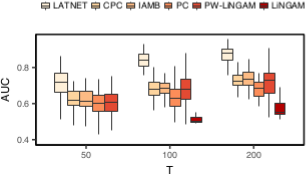
Figure 1: AUC obtained on the brain data ($N=15$) for performing link prediction (connectivity between brain regions) for different number of observations from each node ($T$).

The aim is to discover the connectivity between different brain regions is crucial in neuroscience studies. We analyze the benchmarks of Smith et al. (2011), in which the activity of different brain regions is recorded at different time points and the aim is to find which brain regions are connected to each other. Each benchmark consists of data from 50 subjects, each consisting of 200 time points ($T=200$). We used network sizes $N=5,10,15$, and the true underlying connectivity network is a directed acyclic graph (DAG). Networks discovered by latnet are not restricted to DAGs, and therefore baseline methods assuming the underlying network is a DAG have a de facto favorable bias.

Results are evaluated using the area under the ROC curve (AUC) and shown in Figure 1 for $N=15$ using box-plots (top and bottom edges of the box correspond to the first and third quartiles respectively). The appendix (§10.2) presents details on how the AUC is computed for the different methods and the results for $N=5,10$. We see that, although other methods are favorably biased about the underlying structure, latnet  provides significantly better performance than such baselines. We note that lingam was unable to perform inference for $T$ small and its output is reported only for $T\geq 100$. We also note that pc, cpc and iamb may generate non-concave ROCs. Curves can be post-processed for concave envelopes which improves the AUC, but this artificial post-processing that equivalently mixes outputs does not guarantee the existence of parameters that will in effect produce networks with the corresponding performances. This is discussed in the appendix §10.2, along with the results with concavification.

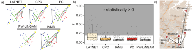
Figure 2: (a) Networks discovered by the different methods. Points in the graph are located according to their geographical coordinates. red: inner ring suburbs; green: middle ring suburbs; blue: outer ring suburbs; yellow: greater metropolitan region. (b) Distribution of $r$ values for each method. $r$ refers to the proportion of the networks in which a discovered arc presents. (c) Arcs with highest $r$ values discovered by latnet.

.

7.3 sydney domain

The aim is to discover the relationship between property prices in different suburbs of Sydney. The data includes quarterly median sale prices for 51 suburbs in Sydney and surrounding area from 1995 to 2014. We kept the analysis window to five years ($T=20$ since data is quarterly) and starting from 1995–1999 the window is shifted by one year each time until 2010-2014. Some major patterns are expected, like the presence of hubs or authorities related to mass transfers between suburbs.

Figure 2(a) shows the inferred arcs for years 2010-2014, where the nodes are positioned according to their geographical locations. See the appendix for the full map of the discovered arcs for all years and for details of the thresholds used for finding significant arcs. We see that the network discovered by latnet is more regionally localized compared to the other methods, and displays major authorities. Note that lingam was unable to perform inference. To complete with a quantitative analysis, we computed for each algorithm and for each pair of nodes, the proportion $r$ of networks in which an arc was discovered. Then, we computed a distribution of the $r$ values in the networks, emphasizing the “stable” arcs with $r$ statistically $>0$ (risk $\alpha=0.05$). Figure 2(b) shows the $r$ values for the different methods. Less than $8\%$, $5\%$ of pc and cpc arcs were significant, respectively, while more than 29$\%$ of latnet arcs are significant. Interestingly, iamb and pw-lingam did not find significant arcs.

What turns out to be interesting is the actual arcs found for those in the 29$\%$ that represent the highest $r$-values. Figure 2(c) shows the top-6 of these arcs inferred by latnet. They clearly indicate that one area of Sydney, Woollahra, acts like an authority in the network, since it receives lots of arcs from other major areas (Hunters Hill, Manly, Mosman, Pittwater). These areas all share common features: they are in central-north Sydney, all have coastal areas, and they happen to be well-known prestigious areas with the highest median property price in Sydney Campion (2011), so the observed percolation is no surprise.

7.4 yeast domain

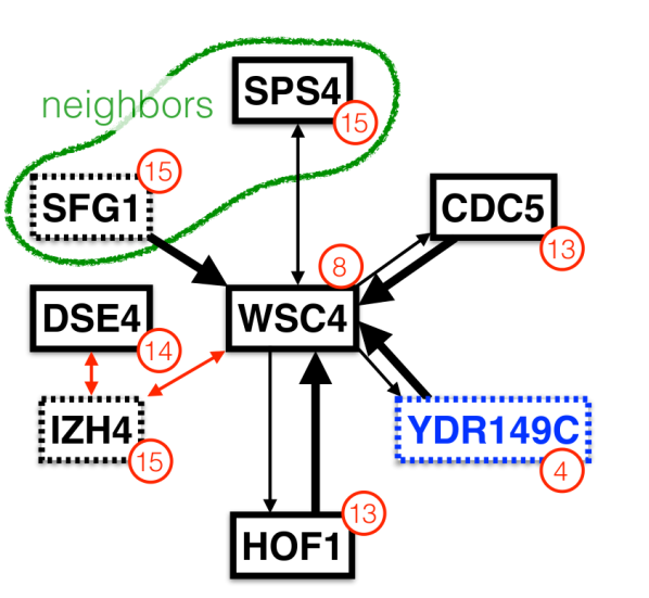
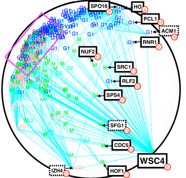
Figure 3: (best viewed in color) Left: subgraph $G_{w}$ containing all strong arcs with $p_{ij}>0.62$; plain rectangles (vs dashed): reported cell cycle transcriptionally regulated genes Rowicka et al. (2007); thick arcs (resp. thin arcs): $p>0.65$ (resp. $p\in(0.62,0.65]$); black arcs (resp red arcs): $\mu>0$ (resp. $\mu<0$); red disk: chromosome number; in blue: gene with no known biological process/function/compartment; Center: manifold learned from strong arcs, displayed in Klein disk (conformal). Strong arcs displayed in blue segments; gene names shown for the most important ones on manifold (conventions follow left pic); pink rectangle: area with comparatively few strong arcs; Right: network aggregating strong arcs discovered for the YCC, between cell cycle phases (see text).

The aim is to infer genome regulation patterns for one extensively studied species, (Saccharomyces cerevisiae, Spellman et al., 1998)’s. In numbers, this represents 100,000+ data points and a network with up to 38,000,000+ arcs. Biology tells us that this network is directed. The complete set of experiments and results is available in the appendix, §10.3. In addition to the full genome analysis, we have performed a finer grained analysis on a $\sim$tenth known to be involved in a heavily regulated and key part of the yeast’s life, the yeast cell cycle (YCC). These genes are the so-called sentinels of the YCC Spellman et al. (1998). In each experiments, we have scrutinized the subset of strong arcs, for which both $p_{ij}$ ($\mathbf{A}$) and $|\mu_{ij}|$ ($\mathbf{W}$) are large, that is, $p_{ij}$ in top-$0.1\%$, $|\mu_{ij}|$ in top-$1\%$. These arcs happen to be indeed very significant, with $\alpha$ risk $\approx 10^{-4}$ for the rejection of hypothesis that $p_{ij}$ is not larger than random existence ($0.5$). The discovered networks’ information is far beyond the scope of this paper, but some striking points can be noted, taking as references the cell cycle transcriptionally regulated genes (Rowicka et al., 2007) and http://www.yeastgenome.org as a more general resource.

Analysis of the YCC. Figure 3 summarizes qualitatively the results obtained by latnet. The topmost strong arcs belong to a small connected component ($G_{w}$) organized around gene WSC4, asymmetric (both in terms of arcs and $p$ values) and with apparent patterns of positive / negative regulation (sign of $\mu$). The key genes are involved in the cell structure dynamics (DSE4, WSC4, CDC5, HOF1). The IZH4 arcs with negative $\mu$ are perhaps not surprising: WSC4 and DSE4 are involved into cell walls (integrity for the former, degradation for the latter). IZH4 is a man-in-the-middle: it has activity elevated in zinc deficient cells, and it turns out that zinc is crucial for hundreds of enzymes, e.g. for protein folding. Strikingly, SPS4 and SFG1 happen to be neighbors on the same chromosome. Figure 3 (center) shows the broad picture, with a display of the manifold coordinates induced by the network’s graph, built upon Meila & Shi (2001). It displays that a small number of key genes drive the coordinates. Most of these genes have been pinned down as cell cycle transcriptionally regulated (Rowicka et al., 2007), and they essentially turn out to be heavily involved in both a/sexual reproduction. Last, Figure 3 (right) summarizes the broad picture of strong arcs between YCC phases: it should come at no surprise that cell splitting, (M)itosis, has the largest number of these arcs.

Analysis of the full genome (results in appendix, 10.4). The following patterns emerge: first, the network is highly asymmetric: more than twice strong arcs go outside the YCC compared to arcs coming in the YCC from non-YCC genes. Second, the leading YCC genes are still major genes, but they tend to be outnumbered by genes that are perhaps more “all-purpose”. Last, the predominance of gap phase G1 compared to G2 is in fact a known feature of Saccharomyces cerevisiae (compared to other yeast species such as Saccharomyces pombe).

8 Conclusion & Discussion

We introduced a framework for network structure discovery when continuous-valued observations from the nodes are given, which can be seen as a generalization of linear causal models. We have established an interesting connection of the model with multi-task learning and developed an efficient variational inference method for estimating the posterior distribution over the network structure. We have demonstrated the benefits of our approach on real applications by providing qualitative and quantitative analyses. Besides computational efficiency, our theoretical analysis shows that the traditional constraints for numerical stability and identifiability in networks are alleviated. Indeed, from a theoretical standpoint, the state of the art goes with substantial constraints that can be related to the fact that the true model exists, is unique and can be properly recovered. Such constraints go with an abstraction of the dynamical model that looks like a series of the type $\sum_{t\geq 0}z^{t}$, where $t$ symbolizes discrete time and $z$ can be a real, complex or matrix argument Hyvärinen & Smith (2013); Linderman & Adams (2014). The trick of replacing the analysis overall $t$s by one over a window, rather than alleviating the constraint, substitutes it for other stationarity constraints that can be equally restrictive Shimizu et al. (2006). In our case, such constraints do not appear because time is absorbed in a GP. The finiteness of the evidence lower-bound (ELBO) is essentially obtained “for free". What we get with additional assumptions that parallel traditional ones is a non-negligible uplift in the easiness of the expected log-likelihood part, the bottleneck of the ELBO. This result also holds for a broader class of posteriors than the ones we use, opening interesting avenues of applications for concrete distributions.

Finally, experiments display that latnet is able to perform sound inference already on small domains, and scales to large domains with the ability to pinpoint meaningful local properties of the networks, as well as capture important high-level network features like global patterns of emigration between wealthy suburbs in Sydney or species characteristics for the yeast.

9 Proofs and algorithms

9.1 Proof of Theorem 1

Figure 4: Sampling graph for arc going from node $n_{j}$ to node $n_{i}$ ($i\neq j$). Grey nodes denote random variables. Notations in part borrowed from Maddison et al. (2016). $\lambda_{c}$ is a constant that does not depend on the arc.

Theorem 5

For any $\lambda_{c}\geq 0$ and $\alpha_{ij}\geq 0$ ($\forall i\neq j$), $\mathbf{I}-\mathbf{B}$ is non-singular with probability one.

Proof: Denote for short $\mathbf{G}\stackrel{{\scriptstyle\text{\tiny def}}}{{=}}\mathbf{I}-\mathbf{B}$. The proof is split in three cases, (I) $\lambda_{c}>0$ and $\alpha_{ij}>0,\forall i\neq j$, (II) $\lambda_{c}=0$ and $\alpha_{ij}>0,\forall i\neq j$, and finally (III) $\lambda_{c}=0$ and $\exists i\neq j,\alpha_{ij}=0$.
(Case I: $\lambda_{c}>0$, $\alpha_{ij}>0,\forall i\neq j$) The coordinates $g_{ij}$ take on constant values $g_{ii}=1$ on the diagonal ($\forall i\in[N]$), and random values $G_{ij}$ outside the diagonal ($i\neq j$). The density of $G_{ij}$ equals $q(A_{ij})\cdot q(W_{ij})$, where $q(W_{ij})\stackrel{{\scriptstyle\text{\tiny def}}}{{=}}\mathcal{N}(\mu_{ij},\sigma_{ij}^{2})$ and $q(A_{ij})\stackrel{{\scriptstyle\text{\tiny def}}}{{=}}\sigma_{\alpha_{ij},\lambda_{c}}(U)$ with

$$\sigma_{\alpha,\lambda_{c}}(U) \stackrel{{\scriptstyle\text{\tiny def}}}{{=}} \frac{1}{1+\exp\left(-\frac{\log\alpha+\log U-\log(1-U)}{\lambda_{c}}\right)}\>\>,$$ (27)

and $U\sim\mathcal{U}(0,1)$ is uniform on interval $(0,1)$ (Maddison et al., 2016). The proof that $\mathbf{G}$ is invertible adapts a standard argument (for example, Tao (2008)). For any $N\geq 2$, denote $\textbf{g}_{1},\textbf{g}_{2},...,\textbf{g}_{N}$ the columns of $\mathbf{G}$, that is, $\mathbf{G}=[\textbf{g}_{1}|\textbf{g}_{2}|...|\textbf{g}_{N}]$. Each of them can be thought of as a random vector where one coordinate takes value 1 with probability 1, an this coordinate is different for all vectors. $\mathbf{G}$ is non invertible iff $\textbf{g}_{1},\textbf{g}_{2},...,\textbf{g}_{N}$ is linearly dependent. Remark that none of the $\textbf{g}_{j}$s can be the null vector, so if $\mathbf{G}$ is not invertible, then

$$\exists j>1 : \textbf{g}_{j}\in\mathrm{span}(\textbf{g}_{1},\textbf{g}_{2},...,\textbf{g}_{j-1})\>\>.$$ (28)

As a consequence,

$$\Pr(\mathrm{det}(\mathbf{G})=0) \leq \sum_{j}\Pr(\textbf{g}_{j}\in\mathrm{span}(\textbf{g}_{1},\textbf{g}_{2},...,\textbf{g}_{j-1}))\>\>,$$ (29)

where the distribution is the product distribution over the columns of $\mathbf{G}$. Fix any $\textbf{g}_{1},\textbf{g}_{2},...,\textbf{g}_{j-1}$ belonging to the respective supports of the columns, and let

$$q_{j} \stackrel{{\scriptstyle\text{\tiny def}}}{{=}} \Pr(\textbf{g}_{j}\in\mathrm{span}(\textbf{g}_{1},\textbf{g}_{2},...,\textbf{g}_{j-1})|\textbf{g}_{1},\textbf{g}_{2},...,\textbf{g}_{j-1})\>\>.$$ (30)

Because the uniform and normal distributions are both absolutely continuous with respect to Lebesgue measure and $\sigma_{\alpha,\lambda_{c}}(x)\leq 1\ll\infty$ (it is also Lipschitz) for any $\alpha>0,\lambda_{c}\neq 0,U\in(0,1)$, so is the density of $G_{ij}$ for any $i\neq j$, and thereby the density of $\textbf{g}_{j}$ for any $j\geq 1$. Along with the fact that $\mathrm{span}(\textbf{g}_{1},\textbf{g}_{2},...,\textbf{g}_{j-1})$ has strictly positive codimension for any $j\leq N$, it comes

$$q_{j} = 0,\forall j\geq 2,\forall\textbf{g}_{1},\textbf{g}_{2},...,\textbf{g}_{j-1}\mbox{ fixed}\>\>.$$ (31)

Integrating over the choices of $\textbf{g}_{1},\textbf{g}_{2},...,\textbf{g}_{j-1}$, we get $\Pr(\textbf{g}_{j}\in\mathrm{span}(\textbf{g}_{1},\textbf{g}_{2},...,\textbf{g}_{j-1}))=0,\forall j\leq N$ and so $\Pr(\mathrm{det}(\mathbf{G})=0)=0$ from ineq. (29). As a consequence, $\mathbf{I}-\mathbf{B}$ is non-singular with probability one, as claimed.
(Case II: $\lambda_{c}=0$, $\alpha_{ij}>0,\forall i\neq j$) this boils down to choosing a Bernoulli $B(p_{ij})$ distribution over $A_{ij}$, corresponding to the limit case $\lambda_{c}\rightarrow 0$ with (Maddison et al., 2016):

$$p_{ij} = \frac{\alpha_{ij}}{1+\alpha_{ij}}\>\>.$$ (32)

In this case, the distribution of $\textbf{g}_{j}$ is not absolutely continuous but a trick allows to truncate the distribution on a subset over which it is absolutely continuous, and therefore reduce to Case I to handle it.
The only atom eventually having non-zero probability is the canonical basis vector $\textbf{1}_{j}$, which has probability $\prod_{i\neq j}(1-p_{ij})$ to be sampled. We now perform a sequence of recursive row-column (row followed by column or the reverse) permutations, starting on $\mathbf{G}$, which by definition do not change its invertibility status but only the sign of its determinant. The first row-column permutation is carried out in such a way that the first column of the new matrix, $\Pi_{1}(\mathbf{G})$, is the first canonical basis vector, $\textbf{1}_{1}$. We then repeat this operation to have the second canonical basis vector in the second column, and so on until until it cannot be done anymore to make appear on the left block a new canonical basis vector. Assuming we have done $N-k$ sequences, we obtain from $\mathbf{G}$ the final matrix $\Pi_{1}(\mathbf{G})$ with:

$$\Pi_{1}(\mathbf{G}) = \left[\begin{array}[]{ccc}\mathbf{I}_{N-k}&|&\mathbf{A}_{(N-k)\times k}\\ \mathbf{0}_{k\times(N-k)}&|&\hat{\mathbf{G}}_{1,k}\end{array}\right]\>\>.$$ (35)

Here, $\hat{\mathbf{G}}_{1,k}\in{\mathbb{R}}^{k\times k}$. Now, we are going to carry out $\Pi_{1}$ again, but on the lower-right block, $\hat{\mathbf{G}}_{1,k}$. Removing dimension-dependent indexes, we obtain matrix

$$\Pi_{2}(\mathbf{G}) = \left[\begin{array}[]{ccc}\mathbf{I}&|&\mathbf{A}\\ \mathbf{0}&|&\Pi_{1}(\hat{\mathbf{G}}_{1})\end{array}\right]$$ (38)

$$= \left[\begin{array}[]{ccc}\mathbf{I}&|&\mathbf{A}_{1}\\ \mathbf{0}&|&\left[\begin{array}[]{ccc}\mathbf{I}&|&\mathbf{A}_{2}\\ \mathbf{0}&|&\hat{\mathbf{G}}_{2}\end{array}\right]\end{array}\right]\>\>.$$ (43)

We then keep on doing the same transformation on block $\hat{\mathbf{G}}_{2}$ until it is not possible anymore. When it is not possible anymore, we know that the current submatrix, say $\hat{\mathbf{G}}_{n}$, does not contain any canonical basis vector as column, as depicted in Figure 5.

Figure 5: Final matrix $\Pi_{n}(\mathbf{G})$ obtained after recursively applying $\Pi_{1}(.)$ to the lower-right block. Here, white blocks mean all-zero, plain dark lines mean all-one, and grey is unspecified.

Lemma 6

$|\mathrm{det}(\mathbf{G})|=|\mathrm{det}(\hat{\mathbf{G}}_{n})|,\forall n\geq 1$.

Proof: We proceed by induction. The key observation is the following standard linear algebra identity. Denoting with a single index the order of a general square matrix, like $\mathbf{A}_{p}$, we have for any $\mathbf{A}_{p}$ non-singular,

$$\left[\begin{array}[]{ccc}\mathbf{A}_{p}&|&\mathbf{B}\\ \mathbf{C}&|&\mathbf{D}_{q}\end{array}\right]\underbrace{\left[\begin{array}[]{ccc}\mathbf{I}_{p}&|&-\mathbf{A}_{p}^{-1}\mathbf{B}\\ \mathbf{0}&|&\mathbf{I}_{q}\end{array}\right]}_{\stackrel{{\scriptstyle\text{\tiny def}}}{{=}}\mathbf{E}} = \underbrace{\left[\begin{array}[]{ccc}\mathbf{I}_{p}&|&\mathbf{0}\\ \mathbf{C}\mathbf{A}_{p}^{-1}&|&\mathbf{I}_{q}\end{array}\right]}_{\stackrel{{\scriptstyle\text{\tiny def}}}{{=}}\mathbf{F}}\left[\begin{array}[]{ccc}\mathbf{A}_{p}&|&\mathbf{0}\\ \mathbf{0}&|&\mathbf{D}-\mathbf{C}\mathbf{A}_{p}^{-1}\mathbf{B}\end{array}\right]\>\>,$$ (52)

for any $p>0,q>0,p+q=n,\mathbf{B}\in{\mathbb{R}}^{p\times q},\mathbf{C}\in{\mathbb{R}}^{q\times p},\mathbf{D}\in{\mathbb{R}}^{q\times q}$. Taking determinants, we note that $\mathrm{det}(\mathbf{E})=\mathrm{det}(\mathbf{F})=1$ because they are triangular with unit diagonal, and so

$$\mathrm{det}\left(\left[\begin{array}[]{ccc}\mathbf{A}_{p}&|&\mathbf{B}\\ \mathbf{C}&|&\mathbf{D}_{q}\end{array}\right]\right) = \mathrm{det}\left(\left[\begin{array}[]{ccc}\mathbf{A}_{p}&|&\mathbf{0}\\ \mathbf{0}&|&\mathbf{D}-\mathbf{C}\mathbf{A}_{p}^{-1}\mathbf{B}\end{array}\right]\right)$$ (57)

$$= \mathrm{det}(\mathbf{A}_{p})\cdot\mathrm{det}(\mathbf{D}-\mathbf{C}\mathbf{A}_{p}^{-1}\mathbf{B})\>\>,$$ (58)

because the right hand-side in eq. (57) is block diagonal. Matching the left hand-side of eq. (57) with eq. (35), so putting $\mathbf{A}_{p}=\mathbf{I}$ and $\mathbf{C}=\mathbf{0}$, we obtain $\mathrm{det}(\Pi_{1}(\mathbf{G}))=\mathrm{det}(\hat{\mathbf{G}}_{1}-\mathbf{0}\mathbf{I}_{N-k}\mathbf{A}_{p})=\mathrm{det}(\hat{\mathbf{G}}_{1})$, and therefore $|\mathrm{det}(\mathbf{G})|=|\mathrm{det}(\hat{\mathbf{G}}_{1})|$. We then just recursively use eq. (52) on the lower-right block ($\hat{\mathbf{G}}_{j}$, for $j=1,2,...,n-1$) and get the statement of the Lemma. (End of the proof of Lemma 6).       
So, $\mathbf{G}$ is invertible iff $\hat{\mathbf{G}}_{n}$ is invertible and:

$$\Pr(\mathrm{det}(\mathbf{G})=0) \leq \Pr(\mathrm{det}(\Pi_{1}(\mathbf{G}))=0)$$ (59)

$$=\Pr(\mathrm{det}(\hat{\mathbf{G}}_{1})=0)$$

$$\leq \Pr(\exists k\in\{2,3,...,N\}:\mathrm{det}(\hat{\mathbf{G}}_{k})=0|\hat{\mathbf{G}}_{k}\in{\mathbb{R}}^{k\times k}\wedge\mathcal{P}(\hat{\mathbf{G}}_{k}))$$

$$\leq \sum_{k=2}^{N}\Pr(\mathrm{det}(\hat{\mathbf{G}}_{k})=0|\hat{\mathbf{G}}_{k}\in{\mathbb{R}}^{k\times k}\wedge\mathcal{P}(\hat{\mathbf{G}}_{k}))\>\>,$$

where $\mathcal{P}(\mathbf{G})$ is the property that no column of $\mathbf{G}$ is a canonical basis vector. Notice the change: no column in $\hat{\mathbf{G}}_{k}$ is allowed to be a canonical basis vector, and therefore the support for the density of the columns of $\hat{\mathbf{G}}_{k}$ is such that its distribution is now absolutely continuous. We are thus left with the same case as in Case I, which yields $\Pr(\mathrm{det}(\hat{\mathbf{G}}_{k})=0|\hat{\mathbf{G}}_{k}\in{\mathbb{R}}^{k\times k}\wedge\mathcal{P}(\hat{\mathbf{G}}_{k}))=0,\forall k\in\{2,3,...,N\}$, and brings $\Pr(\mathrm{det}(\mathbf{G})=0)=0$ as well.
(Case III: $\lambda_{c}\geq 0$, $\alpha_{ij}=0$ for some $i\neq j$) Remark that $\lim_{\alpha\rightarrow 0}\sigma_{\alpha,\lambda_{c}}(x)=0$ if $\lambda_{c}>0$, and if $\lambda_{c}=0$, this boils down from Case II (eq. (32)) to choosing a Bernoulli $B(0)$ distribution over $A_{ij}$, so both cases coincide with $A_{ij}$ being chosen as $B(0)$, implying $G_{ij}=0$. We are left with the same transformation as in Case II — the main difference being that some $G_{ij}$ is surely zero, but it changes nothing to the reasoning done in case II. Therefore, $\Pr(\mathrm{det}(\mathbf{G})=0)=0$ again.       

9.2 Proof of Theorem 2

It comes from Theorem 1 that $\mathbf{G}^{-1}$ can always be computed with probability one with respect to the random sampling of $\mathbf{B}$, and there is no constraint on the parameterization of the concrete distribution for invertibility (Maddison et al., 2016). Interestingly perhaps, the story would be completely different for the invertibility of $\mathbf{B}$, as the argument for cases (II) and (III) break down because with positive probability that would be easy to lower-bound, $\mathbf{B}$ would in fact be not invertible.

The important consequence of Theorem 5 relies on the computation of the log likelihood, which we recall:

$$\log p(\mathbf{y}|\mathbf{W},\mathbf{A}) = -\frac{1}{2}\log|\boldsymbol{\Sigma}_{y}|-\frac{1}{2}\mathbf{y}^{T}\boldsymbol{\Sigma}_{y}^{-1}\mathbf{y}+C\>\>.$$ (60)

We now prove Theorem 2. We recall the main matrix component of eq. (60):

$$\boldsymbol{\Sigma}_{y} = ((\mathbf{I}-\mathbf{B})^{\top}(\mathbf{I}-\mathbf{B}))^{-1}\otimes\mathbf{K}_{t}+\sigma_{f}^{2}(\mathbf{I}-\mathbf{B})^{-1}\mathbf{B}((\mathbf{I}-\mathbf{B})^{-1}\mathbf{B})^{\top}\otimes\boldsymbol{\Sigma}_{\text{I}}+\sigma_{y}^{2}\mathbf{I}\>\>.$$ (61)

We observe that the following two matrices are positive semi-definite: $(\mathbf{I}-\mathbf{B})^{-1}\mathbf{B}((\mathbf{I}-\mathbf{B})^{-1}\mathbf{B})^{\top}$, $\mathbf{K}_{t}$, while $\boldsymbol{\Sigma}_{\text{I}},\mathbf{I},((\mathbf{I}-\mathbf{B})^{\top}(\mathbf{I}-\mathbf{B}))^{-1}$ are positive definite (with probability 1 for that last one, see Theorem 5). Hence, a sufficient condition for the combination in $\boldsymbol{\Sigma}_{y}$ to be positive definite is $\sigma_{y}^{2}>0$, as claimed. This brings the finiteness of $|\log p(\mathbf{y}|\mathbf{W},\mathbf{A})|$ with probability one, and the statement of Theorem 2.

9.3 Proof of Theorem 3

We split the proof in two main parts, the first of which focuses on a simplified version of the model in which the Bernoulli parameter ($\mathbf{A}$) is sampled according to a Dirac — e.g. in the context of inference, from the prior standpoint, it is maximally informed. The results might be useful outside our framework, if $p$ is sampled from a distribution different from the ones we use.

We state the main notations involved in the Theorem. We define the total (squared) expected input (resp. output) to node $i$ as $\mu^{+}_{i.}\stackrel{{\scriptstyle\text{\tiny def}}}{{=}}\sum_{j}\mu_{ij}^{2}$ (resp. $\mu^{+}_{.i}\stackrel{{\scriptstyle\text{\tiny def}}}{{=}}\sum_{j}\mu_{ji}^{2}$), and the total input (resp. output) variance as ${\sigma}^{+}_{i.}\stackrel{{\scriptstyle\text{\tiny def}}}{{=}}\sum_{j}\sigma_{ij}^{2}$ (resp. ${\sigma}^{+}_{.i}\stackrel{{\scriptstyle\text{\tiny def}}}{{=}}\sum_{j}\sigma_{ji}^{2}$). We also define averages, $\overline{\mu}^{+}_{i.}\stackrel{{\scriptstyle\text{\tiny def}}}{{=}}\mu^{+}_{i.}/N$, $\overline{\sigma}^{+}_{i.}\stackrel{{\scriptstyle\text{\tiny def}}}{{=}}\sigma^{+}_{i.}/N$ (same for outputs), and biased weighted proportions, $\tilde{p}^{\mu}_{i.}\stackrel{{\scriptstyle\text{\tiny def}}}{{=}}\sum_{j}p_{ij}\mu_{ij}^{2}/\mu^{+}_{i.}$, $\tilde{p}^{\sigma}_{i.}\stackrel{{\scriptstyle\text{\tiny def}}}{{=}}\sum_{j}p_{ij}\sigma_{ij}^{2}/\sigma^{+}_{i.}$ (again, same for outputs).

Now, we define two functions $U,E:\{1,2,...,2N\}\rightarrow\mathbb{R}_{+}$ as:

$$U(i) \stackrel{{\scriptstyle\text{\tiny def}}}{{=}} \left\{\begin{array}[]{ll}2\tilde{p}^{\mu}_{i.}\overline{\mu}^{+}_{i.}+2\tilde{p}^{\sigma}_{i.}\overline{\sigma}^{+}_{i.}&(i\leq N)\\ 2\tilde{p}^{\mu}_{.j}\overline{\mu}^{+}_{.j}+2\tilde{p}^{\sigma}_{.j}\overline{\sigma}^{+}_{.j}:j\stackrel{{\scriptstyle\text{\tiny def}}}{{=}}i-N&(i>N)\end{array}\right.\>\>,$$

$$E(i) \stackrel{{\scriptstyle\text{\tiny def}}}{{=}} \left\{\begin{array}[]{ll}\phi(\tilde{p}^{\mu}_{i.})\cdot\overline{\mu}^{+}_{i.}+\overline{\sigma}^{+}_{i.}&(i\leq N)\\ \phi(\tilde{p}^{\mu}_{.j})\cdot\overline{\mu}^{+}_{.j}+\overline{\sigma}^{+}_{.j}:j\stackrel{{\scriptstyle\text{\tiny def}}}{{=}}i-N&(i>N)\end{array}\right.\>\>,$$

where $\phi(z)\stackrel{{\scriptstyle\text{\tiny def}}}{{=}}2\sqrt{z(1-z)}$ is Matsushita’s entropy. For any diagonalizable matrix $\mathbf{M}$, we let $\lambda(\mathbf{M})$ denote its eigenspectrum, and $\lambda^{\uparrow}(\mathbf{M})\stackrel{{\scriptstyle\text{\tiny def}}}{{=}}\max\lambda(\mathbf{M})$, $\lambda^{\downarrow}(\mathbf{M})\stackrel{{\scriptstyle\text{\tiny def}}}{{=}}\min\lambda(\mathbf{M})$. Our simplified version of Theorem 3, which we first prove, is the following one.

Theorem 7

Assume $\mathsf{A}_{ij}\sim\mathcal{B}(\uprho_{ij})$ with $\uprho_{ij}\sim\mathrm{Dirac}(p_{ij})$, and $\mathsf{W}_{ij}\sim\mathcal{N}(\mu_{ij},\sigma^{2}_{ij})$, $p_{ij},\mu_{ij},\sigma_{ij}$ being fixed for any $i,j$. Fix any constants $c>0$ and $0<\upgamma<1$ and let

$$\lambda_{\circ}\stackrel{{\scriptstyle\text{\tiny def}}}{{=}}\frac{\lambda^{\downarrow}(\mathbf{K}_{t})}{2}+\sigma_{y}^{2}\>\>,\>\>\lambda_{\bullet}\stackrel{{\scriptstyle\text{\tiny def}}}{{=}}2\lambda^{\uparrow}(\mathbf{K}_{t})+\sigma_{f}^{2}+\sigma_{y}^{2}\>\>.$$ (64)

Suppose that:

$$\max_{i}U(i) \in \left[\frac{\max_{i}E(i)}{N^{\gamma}},\frac{1}{100N^{2}}\right]\>\>.$$ (65)

If $N$ is larger than some constant depending on $c$ and $\gamma$, then with probability $\geq 1-(1/N^{c})$ over the sampling of $\mathbf{W}$ and $\mathbf{A}$, the following holds true:

$$\lambda(\boldsymbol{\Sigma}_{y}) \subset \left[\lambda_{\circ},\lambda_{\bullet}\right]\>\>.$$ (66)

9.3.1 Helper tail bounds and properties for arcs, row and columns in matrix $\mathbf{A}\odot\mathbf{W}$

To obtain concentration bounds on $\log p(\mathbf{y}|\mathbf{W},\mathbf{A})$, we need to map the arc signal onto the real line, including e.g. when $p=0$ (in which case there cannot exist an arc between the two corresponding nodes, so there is no observable "weight" per se). We follow the convention for the Hawkes model of Linderman & Adams (2014), and associate to these "no signal" events the real zero, which makes sense since for example it matches the Dirac case when $\mu,\sigma\rightarrow 0$ — which corresponds to an arc with weight always zero —. Define for short

$$\mathbf{H} \stackrel{{\scriptstyle\text{\tiny def}}}{{=}} (\mathbf{I}-\mathbf{B})^{\top}(\mathbf{I}-\mathbf{B})\>\>,$$ (67)

$$\mathbf{H}^{\prime} \stackrel{{\scriptstyle\text{\tiny def}}}{{=}} (\mathbf{I}-\mathbf{B})(\mathbf{I}-\mathbf{B})^{\top}\>\>,$$ (68)

$$\mathbf{J} \stackrel{{\scriptstyle\text{\tiny def}}}{{=}} \mathbf{B}\mathbf{B}^{\top}\>\>,$$ (69)

so that

$$\boldsymbol{\Sigma}_{y} = \mathbf{H}^{-1}\otimes\mathbf{K}_{t}+\sigma_{f}^{2}(\mathbf{I}-\mathbf{B})^{-1}\mathbf{J}(\mathbf{I}-\mathbf{B})^{-\top}\otimes\boldsymbol{\Sigma}_{\text{I}}+\sigma_{y}^{2}\mathbf{I}\>\>.$$ (70)

We remark that the eigenspectrum of $(\mathbf{I}-\mathbf{B})^{-1}\mathbf{J}(\mathbf{I}-\mathbf{B})^{-\top}$ is the same as for $\mathbf{J}\mathbf{H}^{\prime-1}$: if u is an eigenvector of $(\mathbf{I}-\mathbf{B})^{-1}\mathbf{J}(\mathbf{I}-\mathbf{B})^{-\top}$, then $(\mathbf{I}-\mathbf{B})^{-1}\mathbf{J}(\mathbf{I}-\mathbf{B})^{-\top}\textbf{u}=\lambda\textbf{u}$ is equivalent to $\mathbf{J}(\mathbf{I}-\mathbf{B})^{-\top}\textbf{u}=\lambda(\mathbf{I}-\mathbf{B})\textbf{u}$, equivalent to $\mathbf{J}(\mathbf{I}-\mathbf{B})^{-\top}(\mathbf{I}-\mathbf{B})^{-1}\textbf{v}=\lambda\textbf{v}$ (letting $\textbf{v}\stackrel{{\scriptstyle\text{\tiny def}}}{{=}}(\mathbf{I}-\mathbf{B})\textbf{u}$), finally equivalent to $\mathbf{J}\mathbf{H}^{\prime-1}\textbf{v}=\lambda\textbf{v}$. Therefore, bounding the eigenspectra of $\mathbf{H},\mathbf{H}^{\prime},\mathbf{J}$, plus adequate assumptions on that of $\mathbf{K}_{t}$, shall lead to bounding the eigenspectra of $\boldsymbol{\Sigma}_{y}$, but to get al these bounds, we essentially need properties and concentration inequalities for the coordinates of $\mathbf{B}$ and their row- or column- sums. This is what we establish in this Section.

We first derive a tail bound for arc weight, removing indexes for clarity, and assuming $q(W)\stackrel{{\scriptstyle\text{\tiny def}}}{{=}}\mathcal{N}(\mu,\sigma^{2})$ and $q(A)\stackrel{{\scriptstyle\text{\tiny def}}}{{=}}\mathcal{B}(p)$ (see Figure 4). Let $\mathsf{W}$ denote the random variable taking the arc weight. We recall that random variable $\mathsf{X}$ is $(k,\upbeta)$-sub-Gaussian ($k,\upbeta>0$) iff (Vu, 2014):

$$\mathbb{E}_{\mathsf{X}}[\exp(\uplambda(\mathsf{X}-\mathbb{E}[\mathsf{X}])) \leq k\cdot\exp\left(\frac{\upbeta^{2}\uplambda^{2}}{2}\right)\>\>,\forall\uplambda\in\mathbb{R}\>\>.$$ (71)

Theorem 8

Let $\mathsf{W}\sim q(W)\cdot q(A)$. The following holds true:

$$\mathbb{E}_{\mathsf{W}}[\exp(\uplambda(\mathsf{W}-\mathbb{E}[\mathsf{W}])) = (1-p)\cdot\exp(-p\mu\uplambda)+p\cdot\exp\left(\mu(1-p)\uplambda+\frac{\sigma^{2}\uplambda^{2}}{2}\right)\>\>,\forall\uplambda\in\mathbb{R}\>\>.$$ (72)

Furthermore, $\mathsf{W}$ is $(1,\upbeta)$-sub-Gaussian with $\upbeta$ satisfying:

• $\upbeta^{2}=p\sigma^{2}$ if $p\in\{0,1\}$,

• $\upbeta^{2}=2\sqrt{p(1-p)}\mu^{2}+\sigma^{2}$ if $p\in(0,1)$.

Proof: Denote for short two random variables $\mathsf{N}\sim\mathcal{N}(\mu,\sigma^{2})$ and $\mathsf{B}\sim\mathcal{B}(p)$. We trivially have $\mathbb{E}[\mathsf{W}]=p\mu$ and:

$$\mathbb{E}_{\mathsf{W}}[\exp(\uplambda(\mathsf{W}-\mathbb{E}[\mathsf{W}])) = \mathbb{E}_{\mathsf{W}}[\exp((\mathsf{W}-p\mu)\uplambda)]$$ (73)

$$= (1-p)\cdot\mathbb{E}_{\mathsf{N}}[\exp(-p\mu\uplambda)]+p\cdot\mathbb{E}_{\mathsf{N}}[\exp((\mathsf{N}-p\mu)\uplambda)]$$

$$= (1-p)\cdot\exp(-p\mu\uplambda)+p\cdot\mathbb{E}_{\mathsf{N}}[\exp((\mathsf{N}-p\mu)\uplambda)]$$

$$= (1-p)\cdot\exp(-p\mu\uplambda)+p\cdot\exp(-p\mu\uplambda)\cdot\mathbb{E}_{\mathsf{N}}[\exp(\mathsf{N}\uplambda)]$$

$$= (1-p)\cdot\exp(-p\mu\uplambda)+p\cdot\exp(-p\mu\uplambda)\cdot\exp\left(\mu\uplambda+\frac{\sigma^{2}\uplambda^{2}}{2}\right)$$

$$= (1-p)\cdot\exp(-p\mu\uplambda)+p\cdot\exp\left(\mu(1-p)\uplambda+\frac{\sigma^{2}\uplambda^{2}}{2}\right)\>\>,$$ (74)

for any $\uplambda\in\mathbb{R}$, as claimed for eq. (72). Eq. (73) comes from the moment generating function for Gaussian $\mathsf{N}$. Now, it is clear that

• $\mathsf{W}$ is sub-Gaussian with parameter $\upbeta=\sigma$ in the following two cases: (i) $p=1$, (ii) $\mu=0$. For this latter case, we have indeed $\mathbb{E}_{\mathsf{W}}[\exp(\uplambda(\mathsf{W}-\mathbb{E}[\mathsf{W}]))=(1-p)+p\cdot\exp(\sigma^{2}\uplambda^{2}/2)\leq((1-p)+p)\cdot\exp(\sigma^{2}\uplambda^{2}/2)=\exp(\sigma^{2}\uplambda^{2}/2)$ (using Jensen’s inequality on $z\mapsto\exp(z)$). Furthermore, sub-Gaussian parameter $\sigma$ cannot be improved in both cases.

• the trivial case $p=0$ leads to sub-Gaussianity for any $\upbeta\geq 0$.

Otherwise (assuming thus $0<p<1$ and $\mu\neq 0$), we can immediately rule out the case $\upbeta\leq\sigma$ (for any $k>0$), by noticing that, for $\upbeta=\sigma$, we have $p\cdot\exp(\mu(1-p)\uplambda)=k$ for

$$\uplambda = \frac{1}{(1-p)\mu}\log\frac{k}{p}\>\>(\ll\infty)\>\>,$$ (75)

and so, for this value of $\uplambda$, $\mathbb{E}_{\mathsf{W}}[\exp(\uplambda(\mathsf{W}-\mathbb{E}[\mathsf{W}]))>p\cdot\exp\left(\mu(1-p)\uplambda+(\upbeta^{2}\uplambda^{2})/2\right)=k\exp(\upbeta^{2}\uplambda^{2}/2)$. In the following, we therefore consider $0<p<1$, $\mu\neq 0$ and $\upbeta>\sigma$.

Lemma 9

$\forall p\in[0,1],\forall x>0$, we have

$$p(x-1)+1 \leq x^{p}\exp(\phi_{u}(p)\cdot\log^{2}x)\>\>,$$ (76)

where $\phi_{u}(p)\stackrel{{\scriptstyle\text{\tiny def}}}{{=}}\sqrt{p(1-p)}$ is (unnormalized) Matsushita’s entropy.

Remark: ineq. (76) is probably close to be optimal analytically. Replacing $\phi_{u}(p)$ by a dominated entropy like Gini’s $\phi_{u}(p)\propto p(1-p)$ (i.e. with finite derivatives on the right of 0 and left of 1) seems to break the result.
Proof: The proof makes use of several tricks to counter the fact that the right-hand side of ineq. (76) is essentially concave – but not always – in $p$, and essentially convex – but not always – in $x$, and matches the left-hand side as $p\rightarrow\{0,1\}$. In a first step, we show that ineq. (76) holds for $\log x\in[-1,1]$ (and any $p\in[0,1]$), then Step 2 shows that ineq. (76) holds for $\log x\geq-1$ (and $p\in[0,1]$). Step 3 uses a symmetry argument on the right-hand side of ineq. (76) to extend the result to any $x>0$ (and any $p\in[0,1]$), thereby finishing the proof.

Step 1. We remark that $\phi_{u}(p)\stackrel{{\scriptstyle\text{\tiny def}}}{{=}}\sqrt{p(1-p)}$ satisfies the following properties:

• $\lim_{0}\phi_{u}^{\prime}(p)=+\infty$, $\lim_{1}\phi_{u}^{\prime}(p)=-\infty$;

• $\lim_{\{0,1\}}\phi_{u}^{\prime\prime}(p)+(1+\phi_{u}^{\prime}(p)\cdot k)^{2}=-\infty$ for any $k$.

Denote for short $F(p,x)\stackrel{{\scriptstyle\text{\tiny def}}}{{=}}x^{p}\exp(\phi_{u}(p)\cdot\log^{2}x)$. We have:

$$\frac{\partial F}{\partial p} = \log x\cdot(1+\phi_{u}^{\prime}(p)\cdot\log x)\cdot F_{x}(p)\>\>,$$ (77)

$$\frac{\partial^{2}F}{\partial p^{2}} = \log^{2}x\cdot\left(\phi_{u}^{\prime\prime}(p)+(1+\phi_{u}^{\prime}(p)\log x)^{2}\right)\cdot F_{x}(p)\>\>.$$ (78)

It comes $\partial F/\partial p\sim_{0}\phi_{u}^{\prime}(p)\log^{2}x\cdot F_{x}(p)$ and so $\lim_{0}\partial F/\partial p=+\infty$ because of (i). Since $F(0,x)=1$, we have $F(p,x)>p(x-1)+1$ in a neighborhood of 0. Also, we can check as well that $\lim_{0}\partial^{2}F/\partial p^{2}=-\infty$ because of (ii), so $F(p,x)$ is concave in a neighborhood of $0$. For the same reasons, $F(p,x)$ is concave in a neighborhood of $1$ and since $F(1,x)=x$, we also have $F(p,x)>p(x-1)+1$ in a neighborhood of 1. Now, to zero the second derivative, we need equivalently:

$$\log x = \frac{1}{\phi_{u}^{\prime}(p)}\cdot\left(\frac{\pm 1}{2\phi_{u}^{\frac{3}{2}}(p)}-1\right)\>\>,$$ (79)

or, equivalently again:

$$G(p,x)\stackrel{{\scriptstyle\text{\tiny def}}}{{=}}2\phi_{u}^{\frac{3}{2}}(p)+\log x(1-2p)\phi_{u}^{\frac{1}{2}}(p) = r\>\>,$$ (80)

with $r\in\{-1,1\}$. We have (letting $z\stackrel{{\scriptstyle\text{\tiny def}}}{{=}}\log x$ for short and $h_{1}(z)\stackrel{{\scriptstyle\text{\tiny def}}}{{=}}\sqrt{8z^{2}+9},h_{2}(z)\stackrel{{\scriptstyle\text{\tiny def}}}{{=}}(2z^{2}+h_{1}(z)+3)/(z^{2}+1)$),

$$\max_{p\in[0,1]}G(p,x) = \frac{\left(h_{2}(z)\right)^{\frac{1}{4}}\left(\sqrt{h_{2}(z)(z^{2}+1)}+\sqrt{3+4z^{2}-h_{1}(z)}z\right)}{2^{\frac{5}{4}}3^{\frac{3}{4}}\sqrt{z^{2}+x1}}\>\>,$$ (81)

and we can check that $\max_{p\in[0,1]}G(p,x)<1$ when $\log(x)\leq 1$. We can also check that $\min_{p\in[0,1]}G(p,x)>-1$ when $\log(x)\geq-1$, so eq. (79) has in fact no solution whenever $\log x\in[-1,1]$, regardless of the choice of $r$. Hence, in this case, $F(p,x)$ is concave in $p$ and we get $F(p,x)\geq p(x-1)+1$, for any $\log x\in[-1,1]$.

Step 2. Suppose now that $|\log x|>1$. We have

$$\frac{\partial F}{\partial x} = \frac{1}{x}\cdot\left(p+2\phi_{u}(p)\log x\right)\cdot G_{p}(x)\>\>,$$ (82)

$$\frac{\partial^{2}F}{\partial x^{2}} = \frac{1}{x^{2}}\cdot\left(4\phi_{u}^{2}(p)\log^{2}x+2\phi_{u}(p)(2p-1)\log x+2\phi_{u}(p)-p(1-p)\right)\cdot G_{p}(x)\>\>.$$ (83)

We have $(\partial F/\partial x)(p,1)=p$ and convexity is ensured as long as

$$\log x \not\in \left[\frac{1-2p\pm\sqrt{1-8\phi_{u}(p)}}{4\phi_{u}(p)}\right]\stackrel{{\scriptstyle\text{\tiny def}}}{{=}}\mathcal{A}\>\>.$$ (84)

It happens that $\mathcal{A}\subset[-1,1]$, so whenever $|\log x|\geq 1$, $F(p,x)$ is convex in $x$. To finish Step 2, considering only the case $\log x\geq 1$, it is sufficient to show that $(\partial F/\partial x)(p,e)\geq p$, or equivalently,

$$H(p)\stackrel{{\scriptstyle\text{\tiny def}}}{{=}}\left(p+2\phi_{u}(p)\right)\exp(p+\phi_{u}(p)) \geq ep\>\>,$$ (85)

It can be shown that the first derivative,

$$H^{\prime}(p) = \left(2-p+\frac{2+p-6p^{2}}{2\phi_{u}(p)}\right)\cdot\exp(p+\phi_{u}(p))\>\>,$$ (86)

is $\geq e$ for any $p<0.7$ — so, since both limits in 0 for eq. (85) coincide, eq. (85) holds for any $p<0.7$. The second derivative (fixing $Q(p)\stackrel{{\scriptstyle\text{\tiny def}}}{{=}}2-13p+34p^{2}-12p^{3}-8p^{4}+\phi_{u}(p)((3p-2)(1-4p^{2})+4\phi_{u}^{2}(p)(1-p))$),

$$H^{\prime\prime}(p) = \phi_{u}^{\prime\prime}(p)\cdot Q(p)\cdot\exp(p+\phi_{u}(p))\>\>,$$ (87)

is strictly negative for $p\geq 0.7$ — so, since both limits in 1 for eq. (85) coincide, eq. (85) is strictly concave for $p\geq 0.7$, it sits above its chord $[(0.7,H(0.7)),(1,e)]$ which itself sits above $p\mapsto ep$ for $p\leq 1$, so eq. (85) holds for any $p\geq 0.7$. This achieves the proof of Step 2.

Step 3. We now have that ineq. (76) holds for any $\log x\geq-1$ and any $p\in[0,1]$. To finish the argument, we just have to remark that $F(p,x)$ satisfies the following symmetry:

$$F(p,x) = x\cdot F\left(1-p,\frac{1}{x}\right)\>\>,$$ (88)

so assuming that $\log x<-1$, we have $\log(1/x)\geq 1$, so we reuse Steps 1 and 2 together with eq. (88) to obtain that for any $\log x<-1$,

$$F(p,x) = x\cdot F\left(1-p,\frac{1}{x}\right)$$ (89)

$$\geq x\cdot\left((1-p)\left(\frac{1}{x}-1\right)+1\right)$$

$$=(1-p)(1-x)+x=p(x-1)+1\>\>,$$

as claimed, where the inequality makes use of Steps 1, 2. This achieves the proof of Lemma 9.       
To finish the proof of Theorem 8, we make use of Lemma 9 as follows, starting from eq. (72):

$$\mathbb{E}_{\mathsf{W}}[\exp(\uplambda(\mathsf{W}-\mathbb{E}[\mathsf{W}])) = (1-p)\cdot\exp(-p\mu\uplambda)+p\cdot\exp\left(\mu(1-p)\uplambda+\frac{\sigma^{2}\uplambda^{2}}{2}\right)$$

$$\leq \left\{(1-p)\cdot\exp(-p\mu\uplambda)+p\cdot\exp\left(\mu(1-p)\uplambda\right)\right\}\cdot\exp\left(\frac{\sigma^{2}\uplambda^{2}}{2}\right)$$

$$=\left\{(1-p)+p\cdot\exp\left(\mu\uplambda\right)\right\}\cdot\exp(-p\mu\uplambda)\cdot\exp\left(\frac{\sigma^{2}\uplambda^{2}}{2}\right)$$

$$\leq \exp(p\mu\uplambda)\cdot\exp\left(\phi_{u}(p)\mu^{2}\lambda^{2}\right)\cdot\exp(-p\mu\uplambda)\cdot\exp\left(\frac{\sigma^{2}\uplambda^{2}}{2}\right)$$ (92)

$$=\exp\left(\frac{(\sigma^{2}+2\phi_{u}(p)\mu^{2})\uplambda^{2}}{2}\right)\>\>,\forall\uplambda\in\mathbb{R}\>\>.$$

Ineq. (9.3.1) uses the fact that $\sigma^{2}\uplambda^{2}\geq 0$, and ineq. (92) uses Lemma 9 with $x=\exp(\mu\uplambda)$. Hence, $\mathsf{W}$ is sub-Gaussian with parameters $k=1$ and $\upbeta^{2}=\sigma^{2}+2\phi_{u}(p)\mu^{2}=\sigma^{2}+2\sqrt{p(1-p)}\mu^{2}$, as claimed. This ends the proof of Theorem 8.       
Theorem 8 leads to the following concentration inequality for the row- and column-sums of $\mathbf{B}$, which are key to bound eigenvalues.

Lemma 10

Let $\mu^{+}_{i.}\stackrel{{\scriptstyle\text{\tiny def}}}{{=}}\sum_{j}\mu_{ij}^{2}$, $\mu^{+}_{.j}\stackrel{{\scriptstyle\text{\tiny def}}}{{=}}\sum_{i}\mu_{ij}^{2}$, ${\sigma}^{+}_{i.}\stackrel{{\scriptstyle\text{\tiny def}}}{{=}}\sum_{j}\sigma_{ij}^{2}$, ${\sigma}^{+}_{.j}\stackrel{{\scriptstyle\text{\tiny def}}}{{=}}\sum_{i}\sigma_{ij}^{2}$, and let $\overline{\mu}^{+}_{i.}\stackrel{{\scriptstyle\text{\tiny def}}}{{=}}\mu^{+}_{i.}/N$ (and so on for the other averages $\overline{{\sigma}}^{+}_{i.},\overline{{\sigma}}^{+}_{.j}$). Finally, let $\tilde{p}^{\mu}_{i.}\stackrel{{\scriptstyle\text{\tiny def}}}{{=}}\sum_{j}p_{ij}\mu_{ij}^{2}/\mu^{+}_{i.}$, $\tilde{p}^{\mu}_{.j}\stackrel{{\scriptstyle\text{\tiny def}}}{{=}}\sum_{i}p_{ij}\mu_{ij}^{2}/\mu^{+}_{.j}$ and

$$\nu^{r}_{i} \stackrel{{\scriptstyle\text{\tiny def}}}{{=}} \overline{\mu}^{+}_{i.}\cdot\phi(\tilde{p}^{\mu}_{i.})+\overline{\sigma}^{+}_{i.}\>\>,$$ (93)

$$\nu^{c}_{j} \stackrel{{\scriptstyle\text{\tiny def}}}{{=}} \overline{\mu}^{+}_{.j}\cdot\phi(\tilde{p}^{\mu}_{.j})+\overline{\sigma}^{+}_{.j}\>\>,$$ (94)

where $\phi(p)\stackrel{{\scriptstyle\text{\tiny def}}}{{=}}2\sqrt{p(1-p)}$ is (normalized) Matsushita’s entropy. Then the following holds for any $t>0$:

$$\mathbb{P}\left[\sum_{i}(\mathsf{W}_{ij}-p_{ij}\mu_{ij})\not\in(-Nt,Nt)\right] \leq 2\exp\left(-\frac{Nt^{2}}{2\nu^{c}_{j}}\right)\>\>,$$ (95)

$$\mathbb{P}\left[\sum_{j}(\mathsf{W}_{ij}-p_{ij}\mu_{ij})\not\in(-Nt,Nt)\right] \leq 2\exp\left(-\frac{Nt^{2}}{2\nu^{r}_{i}}\right)\>\>.$$ (96)

Proof: Since the sum of $N$ independent random variables respectively $(k,\upbeta_{i})$-sub-Gaussian ($i\in[N]$) brings a $(k,\sum_{i}\upbeta_{i})$ sub-Gaussian random variable, Theorem 8 immediately yields:

$$\mathbb{P}\left[\frac{1}{N}\sum_{j}(\mathsf{W}_{ij}-\mathbb{E}[\mathsf{W}_{ij}])\geq t\right] \leq \exp\left(-\frac{Nt^{2}}{2\cdot\frac{1}{N}\sum_{j}(2\sqrt{p_{ij}(1-p_{ij})}\mu_{ij}^{2}+\sigma_{ij}^{2})}\right)\>\>.$$ (97)

Since $p\mapsto\sqrt{p(1-p)}$ is concave, we have:

$$\sum_{j}\sqrt{p_{ij}(1-p_{ij})}\mu_{ij}^{2} = \mu^{+}_{i.}\cdot\sum_{j}\frac{\mu_{ij}^{2}}{\mu^{+}_{i.}}\cdot\sqrt{p_{ij}(1-p_{ij})}$$ (98)

$$\leq \mu^{+}_{i.}\cdot\sqrt{\tilde{p}^{\mu}_{i.}\left(1-\tilde{p}^{\mu}_{i.}\right)}\>\>.$$

We finally obtain using ineq. (98),

$$\mathbb{P}\left[\frac{1}{N}\sum_{j}(\mathsf{W}_{ij}-\mathbb{E}[\mathsf{W}_{ij}])\geq t\right] \leq \exp\left(-\frac{Nt^{2}}{2\cdot(\overline{\mu}^{+}_{i.}\cdot 2\sqrt{\tilde{p}^{\mu}_{i.}(1-\tilde{p}^{\mu}_{i.})}+\overline{\sigma}^{+}_{i.})}\right)\>\>,$$ (99)

and we would obtain by symmetry:

$$\mathbb{P}\left[\frac{1}{N}\sum_{j}(\mathsf{W}_{ij}-\mathbb{E}[\mathsf{W}_{ij}])\leq-t\right] \leq \exp\left(-\frac{Nt^{2}}{2\cdot(\overline{\mu}^{+}_{i.}\cdot 2\sqrt{\tilde{p}^{\mu}_{i.}(1-\tilde{p}^{\mu}_{i.})}+\overline{\sigma}^{+}_{i.})}\right)$$ (100)

as well. This ends the proof of Lemma 10.       
Let us define function $E:\{1,2,...,2N\}\rightarrow\mathbb{R}_{+}$ with:

$$E(i) \stackrel{{\scriptstyle\text{\tiny def}}}{{=}} \left\{\begin{array}[]{lcl}2\sqrt{\tilde{p}^{\mu}_{i.}(1-\tilde{p}^{\mu}_{i.})}\cdot\overline{\mu}^{+}_{i.}+\overline{\sigma}^{+}_{i.}&\mbox{ if }&i\leq N\>\>,\\ 2\sqrt{\tilde{p}^{\mu}_{.(i-N)}(1-\tilde{p}^{\mu}_{i.})}\cdot\overline{\mu}^{+}_{.(i-N)}+\overline{\sigma}^{+}_{.(i-N)}&\lx@intercol\mbox{ otherwise }\hfil\lx@intercol\end{array}\right.\>\>,$$ (103)

which collects the key parts in the concentration inequalities for row- / column-sums. We need in fact slightly more than Lemma 10, as we do not just want to bound row- or column-sums, but we need to bound their $L_{1}$ norms (which, since $\|\textbf{u}\|_{1}\geq|\textbf{1}^{\top}\textbf{u}|$ by the triangle inequality, yields a bound on row- or column-sums). It can be verified that $|\mathsf{W}_{ij}|$ is $(2,\upbeta)$-sug-Gaussian with the same $\upbeta$ as for $\mathsf{W}_{ij}$, but because $|\mathsf{W}_{ij}|$ now integrates a folded Gaussian random variable (Tsagris et al., 2014) instead of a Gaussian, its expectation is non trivial. We have not found any (simple) bound on the expectation of such a folded Gaussian, so we provide a complete one here for $\mathsf{W}_{ij}$, which integrates as well Bernoulli parameter $p_{ij}$.

Lemma 11

We have:

$$\mathbb{E}[|\mathsf{W}_{ij}|] \leq p_{ij}\cdot\left(|\mu_{ij}|+\frac{1}{\upgamma}\cdot\frac{\sigma^{2}_{ij}}{\sigma_{ij}+|\mu_{ij}|}\right)\>\>,$$ (104)

where $\upgamma\stackrel{{\scriptstyle\text{\tiny def}}}{{=}}\sqrt{\pi/2}$. Furthermore, (104) is optimal in the sense that both sides coincide when $\mu_{ij}=0$ (in this case, $\mathbb{E}[|\mathsf{W}_{ij}|]=\sigma_{ij}/\upgamma$).

Proof: We now have (removing indices for readability, Tsagris et al. (2014)):

$$\mathbb{E}[|\mathsf{W}|] = p\left(\sqrt{\frac{2}{\pi}}\cdot\sigma\exp\left(-\frac{\mu^{2}}{2\sigma^{2}}\right)+\mu\left[1-2\Phi\left(-\frac{\mu}{\sigma}\right)\right]\right)\>\>,$$ (105)

where $\Phi$ is the CDF of the standard Gaussian, so it is clear that the statement of the Lemma holds (and is in fact tight) when $\mu=0$, as in this case $\mathbb{E}[|\mathsf{W}|]=\sigma\sqrt{2/\pi}$. Otherwise, assume $\mu\neq 0$. For any $z>0$, let

$$f(z) \stackrel{{\scriptstyle\text{\tiny def}}}{{=}} \frac{1}{1+\sqrt{1+\frac{4}{z^{2}}}}\cdot\left(\sqrt{\frac{2}{\pi}}\cdot\frac{1}{z}\exp\left(-\frac{z^{2}}{2}\right)\right)\>\>,$$ (106)

where $u>0$ is a constant. It comes from (Abramowitz & Stegun, 1964, Inequality 7.1.3):

$$\Phi(z) \leq 1-f(z)\>\>,$$ (107)

and so, if $\mu<0$,

$$\mathbb{E}[|\mathsf{W}|] = p\left(\mu+\sqrt{\frac{2}{\pi}}\cdot\sigma\exp\left(-\frac{\mu^{2}}{2\sigma^{2}}\right)-2\mu\Phi\left(-\frac{\mu}{\sigma}\right)\right)$$ (108)

$$\leq p\left(-\mu+\sqrt{\frac{2}{\pi}}\cdot\sigma\exp\left(-\frac{\mu^{2}}{2\sigma^{2}}\right)+2\mu f\left(-\frac{\mu}{\sigma}\right)\right)$$

$$=p\left(|\mu|+\sqrt{\frac{2}{\pi}}\cdot\sigma\exp\left(-\frac{\mu^{2}}{2\sigma^{2}}\right)\left[1-\frac{2}{1+\sqrt{1+\frac{4\sigma^{2}}{\mu^{2}}}}\right]\right)\>\>,$$

and we would obtain the same bound for $\mu>0$. There just remains to remark that ($\forall z>0$):

$$1-\frac{2}{1+\sqrt{1+\frac{1}{z}}} \leq 1-2\sqrt{z}+2z\>\>,$$

$$\left(1-z+\frac{z^{2}}{2}\right)\cdot\exp\left(-\frac{z^{2}}{2}\right) \leq \frac{1}{1+z}\>\>,$$

and we obtain the statement of Lemma 11.       
Using Lemma 11 , we can extend Lemma 10 and obtain the following Lemma.

Lemma 12

Let $E^{\star}\stackrel{{\scriptstyle\text{\tiny def}}}{{=}}\max_{i}E(i)$ and $\mathbb{A}$ denote the event:

$$\mathbb{A}\equiv\left(\exists j\in[N]:\|\textbf{c}_{j}\|_{1}>\sum_{i}p_{ij}(|\mu_{ij}|+\delta_{ij})+Nt\right)\vee\left(\exists i\in[N]:\|\textbf{r}_{i}\|_{1}>\sum_{j}p_{ij}(|\mu_{ij}|+\delta_{ij})+Nt\right)$$ (109)

Then for any $t>0$,

$$\mathbb{P}\left[\mathbb{A}\right] \leq 4N\exp\left(-\frac{Nt^{2}}{2E^{\star}}\right)\>\>,$$ (110)

where $\textbf{r}_{i}\stackrel{{\scriptstyle\text{\tiny def}}}{{=}}(\mathbf{B}\textbf{1})_{i}$ and $\textbf{c}_{j}\stackrel{{\scriptstyle\text{\tiny def}}}{{=}}(\mathbf{B}^{\top}\textbf{1})_{j}$ are respectively row- and column-sums in $\mathbf{B}$, $\delta_{ij}\stackrel{{\scriptstyle\text{\tiny def}}}{{=}}\sigma^{2}_{ij}/(\sigma_{ij}+\upgamma|\mu_{ij}|)$ and $\upgamma\stackrel{{\scriptstyle\text{\tiny def}}}{{=}}\sqrt{\pi/2}$.

The way we use Lemma 12 is the following: pick

$$t = \sqrt{\frac{2E^{\star}}{N}\cdot\log\frac{4N}{\updelta}}\>\>.$$ (111)

We get that with probability $\geq 1-\updelta$, we shall have both

$$\|\textbf{c}_{j}\|_{1} \leq \sum_{i}\tilde{b}_{ij}+\sqrt{2E^{\star}N\cdot\log\frac{8N}{\updelta}}\>\>,\forall j\in[N]\>\>,$$ (112)

$$\|\textbf{r}_{i}\|_{1} \leq \sum_{j}\tilde{b}_{ij}+\sqrt{2E^{\star}N\cdot\log\frac{8N}{\updelta}}\>\>,\forall i\in[N]\>\>,$$ (113)

for all columns and rows in $\mathbf{B}$, with $\tilde{b}_{ij}\stackrel{{\scriptstyle\text{\tiny def}}}{{=}}p_{ij}(|\mu_{ij}|+\delta_{ij})$. There is a balance between the two summands in (112), (113) that we need to clarify to handle the upperbounds. This is achieved through the following Lemma.

Lemma 13

For any $i,j$,

$$\frac{1}{N}\sum_{j}\tilde{b}_{ij} \leq \sqrt{2\tilde{p}^{\mu}_{i.}\overline{\mu}^{+}_{i.}+2\tilde{p}^{\sigma}_{i.}\overline{\sigma}^{+}_{i.}}\>\>,$$

$$\frac{1}{N}\sum_{i}\tilde{b}_{ij} \leq \sqrt{2\tilde{p}^{\mu}_{.j}\overline{\mu}^{+}_{.j}+2\tilde{p}^{\sigma}_{.j}\overline{\sigma}^{+}_{.j}}\>\>,$$

where $\tilde{p}^{\sigma}_{i.}\stackrel{{\scriptstyle\text{\tiny def}}}{{=}}\sum_{j}p_{ij}\sigma_{ij}^{2}/\sigma^{+}_{i.}$, $\tilde{p}^{\sigma}_{.j}\stackrel{{\scriptstyle\text{\tiny def}}}{{=}}\sum_{i}p_{ij}\sigma_{ij}^{2}/\sigma^{+}_{.j}$.

Proof: We have for any $i,j$,

$$\left(\frac{1}{N}\sum_{j}\tilde{b}_{ij}\right)^{2} = \left(\frac{1}{N}\cdot\sum_{j}p_{ij}|\mu_{ij}|\left(1+\frac{\sigma_{ij}}{|\mu_{ij}|}\cdot\frac{1}{1+\upgamma\frac{|\mu_{ij}|}{\sigma_{ij}}}\right)\right)^{2}$$ (114)

$$\leq \left(\frac{1}{N}\cdot\sum_{j}p_{ij}|\mu_{ij}|+\frac{1}{N}\cdot\sum_{j}p_{ij}\sigma_{ij}\right)^{2}$$

$$\leq 2\left(\frac{1}{N}\cdot\sum_{j}p_{ij}|\mu_{ij}|\right)^{2}+2\left(\frac{1}{N}\cdot\sum_{j}p_{ij}\sigma_{ij}\right)^{2}$$

$$\leq 2\sum_{j}p^{2}_{ij}\mu^{2}_{ij}+2\sum_{j}p^{2}_{ij}\sigma^{2}_{ij}$$ (115)

$$\leq 2\sum_{j}p_{ij}\mu^{2}_{ij}+2\sum_{j}p_{ij}{\sigma}^{2}_{ij}$$ (117)

$$=2\tilde{p}^{\mu}_{i.}\overline{\mu}^{+}_{i.}+2\tilde{p}^{\sigma}_{i.}\overline{\sigma}^{+}_{i.}\>\>.$$

Ineqs (114) and (115) follows from $(\sum_{u=1}^{v}a_{u})^{2}\leq v\sum_{u}a_{u}^{2}$. Ineq. (117) comes from $p_{ij}\in[0,1]$. We would have similarly

$$\left(\frac{1}{N}\sum_{i}\tilde{b}_{ij}\right)^{2} \leq 2\tilde{p}^{\mu}_{.j}\overline{\mu}^{+}_{.j}+2\tilde{p}^{\sigma}_{.j}\overline{\sigma}^{+}_{.j}\>\>.$$ (118)

This ends the proof of Lemma 13.       

9.3.2 Proof of Theorem 7

Let us define function $U:\{1,2,...,2N\}\rightarrow\mathbb{R}_{+}$ with:

$$U(i) = \left\{\begin{array}[]{lcl}2\tilde{p}^{\mu}_{i.}\overline{\mu}^{+}_{i.}+2\tilde{p}^{\sigma}_{i.}\overline{\sigma}^{+}_{i.}&\mbox{ if }&i\leq N\>\>,\\ 2\tilde{p}^{\mu}_{.(i-N)}\overline{\mu}^{+}_{.(i-N)}+2\tilde{p}^{\sigma}_{.(i-N)}\overline{\sigma}^{+}_{.(i-N)}&\lx@intercol\mbox{ otherwise }\hfil\lx@intercol\end{array}\right.\>\>,$$ (121)

which collects the bounds in ineqs (117) and (118), and let $U^{\star}\stackrel{{\scriptstyle\text{\tiny def}}}{{=}}\max_{i}U(i)$. Let

$$\ell \stackrel{{\scriptstyle\text{\tiny def}}}{{=}} N\sqrt{U^{\star}}+\sqrt{2E^{\star}N\cdot\log\frac{4N}{\updelta}}\>\>.$$ (122)

$\ell$ is be the quantity we need to handle all eigenspectra, but for this objective, let us define assumption (Z) as:

• $(1+\epsilon)N\sqrt{U^{\star}}\leq 1/5$ (call it the domination assumption for short) and

  $$\frac{E^{\star}}{U^{\star}} \leq \epsilon^{2}\cdot\frac{N}{2\log\frac{4N}{\updelta}}\>\>.$$ (123)

Assumption (Z) is a bit technical: we replace it by a simpler one, (A), which implies (Z). Suppose ${\gamma}\in(0,1)$ a constant, and assume $N\geq K^{1/(1-\gamma)}$ without loss of generality; fix for some constant $c>0$,

$$\updelta = \frac{1}{N^{c}}\>\>,$$ (124)

$$\epsilon^{2} = \frac{2}{N^{1-{\gamma}}}\cdot\log\frac{4N}{\updelta}$$ (125)

$$\geq \frac{2(c+4)}{N^{1-{\gamma}}}\cdot\log N\>\>.$$

Condition (123) is now ensured provided

$$U^{\star} \geq \frac{1}{N^{\gamma}}\cdot E^{\star}\>\>,$$ (126)

while the domination condition is ensured, with $N=\Omega(c^{2+\kappa})$ ($\kappa>0$ a constant) large enough so that $\epsilon\leq 1$, as long as

$$U^{\star} \leq \frac{1}{100N^{2}}\>\>.$$ (127)

So let us simplify assumption (Z) by the following assumption, which implies (Z):

• $c>0$ and $0<\gamma<1$ being constants such that $N=\Omega(poly(c),3^{1/(1-\gamma)})$, we have:

  $$U^{\star} \in \left[\frac{E^{\star}}{N^{\gamma}},\frac{1}{100N^{2}}\right]\>\>.$$ (128)

Again, (A) implies (Z).

Remark 1: the upperbound of (128) is quantitatively not so different from Linderman & Adams (2014)’s assumptions. They work with two assumptions, the first of which being $\displaystyle\sigma^{2}$ $\displaystyle\leq$ $\displaystyle\frac{1}{N}$ (129) (we consider variances for the assumption to rely on same scales as ours), and also pick network parameters $\mu,\sigma$ in such a way that large deviations for edge weights are controlled with high probability, with a condition that roughly looks like: $\displaystyle\mu^{2}+\frac{c}{N^{2}}\cdot\sigma^{2}$ $\displaystyle=$ $\displaystyle O\left(\frac{1}{N^{2}}\right)\>\>,$ (130) for some constant $c>3$. This constraint is relevant to the same stability issues as the ones we study here, and can be found in a slightly different form (but equivalent) in (Hyvärinen & Smith, 2013, Section 4), where it is mandatory for the estimation of ICA model parameters.. Finally, (Linderman & Adams, 2014) make the heuristic choice to enforce at least one of the two ineqs. (129, 130). Remark 2: the sampling constraint akin to eq. (130) is in fact very restrictive for ICA estimation of models (Hyvärinen & Smith, 2013, Section 4), since typically each coordinate in $\mathbf{B}$ has to be bounded with high probability, whereas in our case, it is sufficient to control sums ($L_{1}$, row- or column-wise) with high probability. We can therefore benefit from concentration properties on large networks that such approaches may not have.

What is interesting from (128) is the hints that provide the lowerbound of (128) for Theorem 7 (main file) to hold. The main difference between $U^{\star}$ and $E^{\star}$ is indeed (omitting factor $2\cdot\tilde{p}^{\sigma}\in[0,1]$ in variance terms) the switch between $z\mapsto 2z$ (for $U(.)$) and $z\mapsto\phi(z)$ (for $E(.)$). Figure 6 explains that the lowerbound may be violated essentially only on networks with very unlikely arcs almost everywhere, because $\phi$ has infinite derivative as $z\rightarrow 0$. Also, it gives a justification for the name of the two functions $E$ and $U$, where maximizing $E$ tends to favor arcs with $p$ close to $1/2$ ($E$ stands for Equivocal), while maximizing $U$ tends to favor arcs with $p$ close to $1$ ($U$ stands for Unequivocal).

Figure 6: Region (red cartouche) for which the lowerbound in (128) may fail because $\phi(z)$ happens to be much larger than $2z$ — a worst case corresponding to networks where basically all $p$s are very small (e.g. $o(1/poly(N))$). The Figure also depicts the location of $p$ for "ideal" maximizers of $E(.)$ (hence the name, Equivocal arcs) and $U(.)$ (hence the name, Unequivocal arcs).

($\star$) We now have all we need to bound the eigenspectra of $\mathbf{H},\mathbf{H}^{\prime}$. Let $\lambda^{\uparrow}(.)$ (resp. $\lambda^{\downarrow}(.)$) denote the maximal (resp. minimal) eigenvalue of the argument matrix. We obtain that with probability $\geq 1-\updelta$,

$$\lambda^{\uparrow}(\mathbf{H}) \leq 1+\max_{j}\textbf{c}^{\top}_{j}\sum_{k}\textbf{c}_{k}-(\textbf{r}_{j}+\textbf{c}_{j})^{\top}\textbf{1}$$

$$\leq 1+\max_{j}\|\textbf{c}_{j}\|_{1}\max_{k}|\textbf{1}^{\top}\textbf{r}_{k}|-(\textbf{r}_{j}+\textbf{c}_{j})^{\top}\textbf{1}$$

$$\leq 1+\max_{j}\|\textbf{c}_{j}\|_{1}\max_{i}\|\textbf{r}_{i}\|_{1}+\max_{j}\|\textbf{c}_{j}\|_{1}+\max_{i}\|\textbf{r}_{i}\|_{1}$$

$$\leq \left(1+\ell\right)^{2}\>\>,$$

(ineq. (9.3.2) comes from Hölder inequality) and similarly for the minimal eigenvalue,

$$\lambda^{\downarrow}(\mathbf{H}) \geq 1+\min_{j}\textbf{c}^{\top}_{j}\sum_{k}\textbf{c}_{k}-(\textbf{r}_{j}+\textbf{c}_{j})^{\top}\textbf{1}$$

$$\geq 1-\ell^{2}-2\ell\>\>,$$

which implies that $\ell\leq\sqrt{2}-1$ for this latter bound not to be vacuous ($\ell$ is defined in eq. (122)). As long as $\updelta=\Omega(1/poly(N))$, it is not hard to see that $N\sqrt{U^{\star}}$ dominates in $\ell$ for large networks so we can assume $N$ large enough so that, for some small $\epsilon>0$,

$$\frac{E^{\star}}{U^{\star}} \leq \epsilon^{2}\cdot\frac{N}{2\log\frac{4N}{\updelta}}\>\>,$$ (132)

which brings $\ell\leq(1+\epsilon)N\sqrt{U^{\star}}$. In this case, if $(1+\epsilon)N\sqrt{U^{\star}}\leq 1/5$, then $\lambda^{\downarrow}(\mathbf{H})\geq 1/2$. Furthermore, it is not hard to check that we also get $\lambda^{\uparrow}(\mathbf{H})\leq 3/2$. To summarize, as long as assumption (Z) (and so, as long as (A)) holds, the complete eigenspectra of $\mathbf{H}$, $\mathbf{H}^{-1}$ and by extension $\mathbf{H}^{\prime}$, $\mathbf{H}^{\prime-1}$, all lie within $[1/2,2]$ with high probability.

($\star$) We finish with the eigenspectrum of $\mathbf{J}$. We also easily obtain that

$$\lambda^{\uparrow}(\mathbf{J}) \leq \max_{j}\textbf{r}^{\top}_{j}\sum_{k}\textbf{r}_{k}$$

$$\leq \max_{j}\|\textbf{r}_{j}\|_{1}\max_{k}|\textbf{1}^{\top}\textbf{c}_{k}|$$

$$\leq \ell^{2}\>\>,$$

and obviously $\lambda^{\downarrow}(\mathbf{J})\geq 0$, which is all we need.

($\star$) We now finish the proof of Theorem 7, recalling that $\boldsymbol{\Sigma}_{y}$ can be summarized as:

$$\boldsymbol{\Sigma}_{y} = \mathbf{A}+\sigma_{f}^{2}\mathbf{B}+\sigma_{y}^{2}\mathbf{I}\>\>,$$ (133)

with $\mathbf{A}\stackrel{{\scriptstyle\text{\tiny def}}}{{=}}\mathbf{H}^{-1}\otimes\mathbf{K}_{t}$ has an eigensystem which is the (Minkowski) product of the eigensystems of its two matrices, and therefore is within $[\lambda^{\downarrow}(\mathbf{K}_{t})/2,2\lambda^{\uparrow}(\mathbf{K}_{t})]$; on the other hand, $\mathbf{B}\stackrel{{\scriptstyle\text{\tiny def}}}{{=}}(\mathbf{I}-\mathbf{B})^{-1}\mathbf{J}(\mathbf{I}-\mathbf{B})^{-\top}\otimes\boldsymbol{\Sigma}_{\text{I}}$ has eigensystem which is the one of $\mathbf{J}\mathbf{H}^{\prime}$ (eigenvalues have different algebraic multiplicity though), which therefore is within $[0,\ell^{2}\cdot(1+\ell)^{2}]\subset[0,2/25]$. Hence, simplifying a bit, we can bound the complete eigenspectrum of $\boldsymbol{\Sigma}_{y}$, $\lambda(\boldsymbol{\Sigma}_{y})$, as:

$$\lambda(\boldsymbol{\Sigma}_{y}) \subset \left[\frac{\lambda^{\downarrow}(\mathbf{K}_{t})}{2}+\sigma_{y}^{2},2\lambda^{\uparrow}(\mathbf{K}_{t})+\sigma_{f}^{2}+\sigma_{y}^{2}\right]\>\>,$$ (134)

under assumption (A), with probability $\geq 1-\updelta=1-1/N^{c}$, as claimed. This ends the proof of Theorem 7.

9.3.3 From Theorem 7 to Theorem 3

We now assume $\mathsf{A}\sim\mathcal{B}(\uprho_{ij})$ with $\uprho_{ij}\sim\mathcal{V}_{ij}(p_{ij})$, where $\mathcal{V}$ is a random variable satisfying $p_{ij}\stackrel{{\scriptstyle\text{\tiny def}}}{{=}}\mathbb{E}[\mathcal{V}_{ij}]$ and $\mathrm{supp}(\mathcal{V})\subseteq[0,1]$ (the support of $\mathcal{V}$). The proof essentially follows that of Theorem 7, with the following minor changes.

($\star$) The derivation of eq. (74) now satisfies, since $\phi_{u}(z)$ is maximal in $z=1/2$,

$$\mathbb{E}_{\mathsf{W}_{ij}}[\exp(\uplambda(\mathsf{W}_{ij}-\mathbb{E}[\mathsf{W}_{ij}]))] \leq \int_{\mathrm{Supp}(\mathcal{V})}\exp\left(\frac{(\sigma_{ij}^{2}+2\phi_{u}(z)\mu_{ij}^{2})\uplambda^{2}}{2}\right)\mathrm{d}\mu(z)$$ (135)

$$\leq \exp\left(\frac{(\sigma_{ij}^{2}+2\phi_{u}(1/2)\mu_{ij}^{2})\uplambda^{2}}{2}\right)=\exp\left(\frac{(\sigma_{ij}^{2}+\mu_{ij}^{2})\uplambda^{2}}{2}\right)\>\>.$$

($\star$) Assumption (A) now reads, for some constants $c>0$ and $0<\gamma<1$ such that $N=\Omega(poly(c),3^{1/(1-\gamma)})$, we have:

$$U^{\star} \in \left[\frac{S^{\star}}{N^{\gamma}},\frac{1}{100N^{2}}\right]\>\>,$$ (136)

where $U$ does not change but

$$S(i) \stackrel{{\scriptstyle\text{\tiny def}}}{{=}} \left\{\begin{array}[]{ll}\overline{\mu}^{+}_{i.}+\overline{\sigma}^{+}_{i.}&(i\leq N)\\ \overline{\mu}^{+}_{.j}+\overline{\sigma}^{+}_{.j}:j\stackrel{{\scriptstyle\text{\tiny def}}}{{=}}N-i&(i>N)\end{array}\right.\>\>.$$

9.4 Marginal Likelihood Given the Network Parameters

When calculating the expected log-likelihood it is easier to work with the inverse model:

$$z_{i}(t) \sim\mathcal{GP}(\mathbf{0},\kappa(t,t^{\prime};\boldsymbol{\theta})),$$ (138)

$$\boldsymbol{\epsilon}_{f} \sim\mathcal{N}(0,\sigma_{f}^{2}\mathbf{I})$$ (139)

$$\epsilon_{y} \sim\mathcal{N}(0,\sigma_{y}^{2})$$ (140)

$$f_{i}(t) \sim[{\mathbf{G}}]_{i,:}\left(\mathbf{z}(t)+\mathbf{B}\boldsymbol{\epsilon}_{f}\right)\text{,}$$ (141)

$$y_{i}(t) \sim f_{i}(t)+\epsilon_{y}\text{.}$$ (142)

where $\mathbf{B}=\mathbf{A}\odot\mathbf{W}$; $\mathbf{G}=(\mathbf{I}-\mathbf{B})^{-1}$; $[{\mathbf{M}}]_{i,:}$ denotes the $i\text{th}$ row of matrix $\mathbf{M}$. Here we analyse the conditional likelihood by integrating out everything but $\mathbf{A},\mathbf{W}$. Clearly, for fixed $\mathbf{A},\mathbf{W}$, since all the distributions are Gaussians, and we are only applying linear operators, the resulting distribution over $f_{i}$, and consequently over $y_{i}$, is also a Gaussian process. Hence, we only need to figure out the mean function and the covariance function of the resulting process. For the expectation we have that:

$$\mu_{i}(t)=\mathbb{E}\left[f_{i}(t)\right]=0\text{,}$$ (143)

since both $\mathbf{z}$ and $\epsilon_{f}$ are zero-mean processes. For the covariance function we have that:

$$\mathbb{C}\text{ov}[f_{i}(t),f_{j}(t^{\prime})] =\mathbb{E}\left[(f_{i}(t)-\mu_{i}(t))(f_{j}(t)-\mu_{j}(t^{\prime}))\right]$$ (144)

$$={[\mathbf{G}\mathbf{G}^{T}]_{i,j}}\kappa(t,t^{\prime};\boldsymbol{\theta})+{[\mathbf{G}\mathbf{B}\mathbf{B}^{T}\mathbf{G}^{T}]_{i,j}}\sigma_{f}^{2}$$ (145)

$$={[\mathbf{K}_{f}]_{i,j}}\kappa(t,t^{\prime};\boldsymbol{\theta})+{[\mathbf{E}]_{i,j}}\sigma_{f}^{2}\text{,}$$ (146)

where we have defined ${[\mathbf{M}]_{i,j}}$ the $i,j$ entry of matrix $\mathbf{M}$ and the matrix of latent node covariances and noise covariances as:

$$\mathbf{K}_{f} ={\mathbf{G}}{\mathbf{G}}^{T}$$ (147)

$$\mathbf{E} =\mathbf{G}\mathbf{B}\mathbf{B}^{T}\mathbf{G}^{T}\text{.}$$ (148)

The covariance function of the observations is then given by:

$$\mathbb{C}\text{ov}[y_{i}(t),y_{j}(t^{\prime})] ={[\mathbf{K}_{f}]_{i,j}}\kappa(t,t^{\prime};\boldsymbol{\theta})+{[\mathbf{E}]_{i,j}}\sigma_{f}^{2}+\delta_{ij}\sigma_{y}^{2}\text{.}$$ (149)

For further understanding of this model, let us assume that the observations lie on a grid in time, $t=1,\ldots,T$ and $\mathbf{Y}$ is a $N\times T$ matrix of observations with $\mathbf{y}=\text{vec}{\mathbf{Y}}$ hence the likelihood of all observations is:

$$p(\mathbf{y}|\mathbf{W},\mathbf{A}) =\mathcal{N}(\mathbf{y};\mathbf{0},\boldsymbol{\Sigma}_{y})\text{, with}$$ (150)

$$\boldsymbol{\Sigma}_{y} =\mathbf{K}_{f}\otimes\mathbf{K}_{t}+\mathbf{E}\otimes\sigma_{f}^{2}\mathbf{I}+\mathbf{I}\otimes\sigma_{y}^{2}\mathbf{I}\text{,}$$ (151)

where $\otimes$ denotes the Kronecker product; If we use this setting then we obtain:

$$\boldsymbol{\Sigma}_{y} =\mathbf{K}_{f}\otimes\mathbf{K}_{t}+(\sigma_{f}^{2}\mathbf{E}+\sigma_{y}^{2}\mathbf{I})\otimes\mathbf{I}\text{.}$$ (152)

Interestingly, the model above has been studied in statistics and in machine learning, see e.g. Bonilla et al. (2008); Rakitsch et al. (2013). Furthermore, inference and hyperparameter estimation can be done efficiently by exploiting properties of the Kronecker product, e.g. an evaluation of the marginal likelihood can be done in $\mathcal{O}(N^{3}+T^{3})$. Nevertheless, unless there is a substantial overlapping between the locations of the observations across the nodes (i.e. times), the Kronecker formulation becomes intractable.

9.5 Marginal likelihood

Assuming the general case (i.e. non-grid observations), let us refer to $\boldsymbol{\Sigma}_{y}=\mathbf{K}+\sigma_{y}^{2}\mathbf{I}$ as the covariance of the marginal process over $\mathbf{y}$, as induced by the covariance function in Equation (149), where $\mathbf{K}$ is the covariance matrix induced by the covariance function in Equation (146). Therefore, the prior, conditional likelihood, and marginal likelihood of the model are:

$$p(\mathbf{f}) =\mathcal{N}(\mathbf{f};\mathbf{0},\mathbf{K})\text{,}$$ (153)

$$p(\mathbf{y}|\mathbf{f}) =\mathcal{N}(\mathbf{y};\mathbf{f},\sigma_{y}^{2}\mathbf{I})\text{,}$$ (154)

$$p(\mathbf{y}) =\mathcal{N}(\mathbf{y};\mathbf{0},\boldsymbol{\Sigma}_{y})\text{,}$$ (155)

where we have omitted the dependencies of the above equation on the network parameters $\mathbf{A},\mathbf{W}$. Because of the marginalization property of GPs it is easy to see that all the above distributions are $n$-dimensional, where $n=\sum_{i=1}^{N}T$, where $T$ is the number of observations per node. Hence the cost of evaluating the exact marginal likelihood is $\mathcal{O}(n^{3})$.

9.6 Efficient Computation of Marginal Likelihood Given Network Parameters

For simplicity, we consider here the synchronized case where all the $N$ nodes in the network have $T$ observations at the same times. i.e. the total number of observations is $n=N\times T$. Here we show an efficient expression for the log marginal likelihood:

$$\log p(\mathbf{y}|\mathbf{W},\mathbf{A}) =-\frac{n}{2}\log(2\pi)-\frac{1}{2}\log|\boldsymbol{\Sigma}_{y}|-\frac{1}{2}\mathbf{y}^{T}\boldsymbol{\Sigma}_{y}^{-1}\mathbf{y}\text{, where}$$ (156)

$$\boldsymbol{\Sigma}_{y} =\mathbf{K}_{f}\otimes\mathbf{K}_{t}+\boldsymbol{\Omega}\otimes\boldsymbol{\Sigma}_{\text{I}}\text{, with }$$ (157)

$$\boldsymbol{\Omega} =(\sigma_{f}^{2}\mathbf{E}+\sigma_{y}^{2}\mathbf{I})\text{ and}$$ (158)

$$\boldsymbol{\Sigma}_{\text{I}} =\mathbf{I}$$ (159)

The main difficulty of computing this expression is the calculation of the log determinant of an $n$ dimensional matrix, as well as solving an $n$-dimensional system of linear equations. Our goal is to show that we never need to solve these operations on an $n$-dimensional matrix, which are $\mathcal{O}(n^{3})$ but instead use $\mathcal{O}(N^{3}+T^{3})$ operations.

Given the eigen-decomposition of the above matrices

$$\boldsymbol{\Omega} =\mathbf{Q}_{\Omega}\mathbf{\Lambda}_{\Omega}\mathbf{Q}_{\Omega}^{T}$$ (160)

$$\boldsymbol{\Sigma}_{\text{I}} =\mathbf{Q}_{\text{I}}\mathbf{\Lambda}_{\text{I}}\mathbf{Q}_{\text{I}}^{T}=\mathbf{I}\text{,}$$ (161)

It is possible to show that the marginal covariance is given by

$$\boldsymbol{\Sigma}_{y} =(\mathbf{Q}_{\Omega}\mathbf{\Lambda}_{\Omega}^{1/2}\otimes\mathbf{Q}_{\text{I}}\mathbf{\Lambda}_{\text{I}}^{1/2})\left(\tilde{\mathbf{K}}_{f}\otimes\tilde{\mathbf{K}}_{t}+\mathbf{I}\otimes\mathbf{I}\right)(\mathbf{Q}_{\Omega}\mathbf{\Lambda}_{\Omega}^{1/2}\otimes\mathbf{Q}_{\text{I}}\mathbf{\Lambda}_{\text{I}}^{1/2})^{T}\text{, where}$$ (162)

$$\tilde{\mathbf{K}}_{f} =\mathbf{\Lambda}_{\Omega}^{-1/2}\mathbf{Q}_{\Omega}^{T}\mathbf{K}_{f}\mathbf{Q}_{\Omega}\mathbf{\Lambda}_{\Omega}^{-1/2}$$ (163)

$$\tilde{\mathbf{K}}_{t} =\mathbf{\Lambda}_{\text{I}}^{-1/2}\mathbf{Q}_{\text{I}}^{T}\mathbf{K}_{t}\mathbf{Q}_{\text{I}}\mathbf{\Lambda}_{\text{I}}^{-1/2}=\mathbf{K}_{t}$$ (164)

For these matrices we also define their eigen-decomposition analogously to above:

$$\tilde{\mathbf{K}}_{f} =\tilde{\mathbf{Q}}_{f}\tilde{\lambda}_{f}\tilde{\mathbf{Q}}_{f}^{T}$$ (165)

$$\tilde{\mathbf{K}}_{t} =\mathbf{K}_{t}=\tilde{\mathbf{Q}}_{t}\tilde{\lambda}_{t}\tilde{\mathbf{Q}}_{t}^{T}$$ (166)

9.6.1 Log-determinant Term

$$\log|\boldsymbol{\Sigma}_{y}| =\log|\boldsymbol{\Omega}\otimes\boldsymbol{\Sigma}_{\text{I}}|+\log|\tilde{\mathbf{K}}_{f}\otimes\tilde{\mathbf{K}}_{t}+\mathbf{I}\otimes\mathbf{I}|$$ (167)

$$=T\sum_{i=1}^{N}\log\lambda_{n}^{(i)}+N\sum_{j=1}^{T}\log\lambda_{\text{I}}^{(j)}+\sum_{i=1}^{N}\sum_{j=1}^{T}\log(\tilde{\lambda}_{f}^{(i)}\tilde{\lambda}_{t}^{(j)}+1)$$ (168)

$$=T\sum_{i=1}^{N}\log\lambda_{n}^{(i)}+\sum_{i=1}^{N}\sum_{j=1}^{T}\log(\tilde{\lambda}_{f}^{(i)}\tilde{\lambda}_{t}^{(j)}+1)$$ (169)

9.6.2 Quadratic Term

$$\mathbf{y}^{T}\boldsymbol{\Sigma}_{y}^{-1}\mathbf{y} =\mathbf{y}^{T}(\mathbf{\Lambda}_{\Omega}^{1/2}\mathbf{Q}_{\Omega}^{T}\otimes\mathbf{\Lambda}_{\text{I}}^{1/2}\mathbf{Q}_{\text{I}}^{T})^{-1}\left(\tilde{\mathbf{K}}_{f}\otimes\tilde{\mathbf{K}}_{t}+\mathbf{I}\otimes\mathbf{I}\right)^{-1}(\mathbf{Q}_{\Omega}\mathbf{\Lambda}_{\Omega}^{1/2}\otimes\mathbf{Q}_{\text{I}}\mathbf{\Lambda}_{\text{I}}^{1/2})^{-1}\mathbf{y}$$ (170)

$$\mathbf{y}^{T}\boldsymbol{\Sigma}_{y}^{-1}\mathbf{y} =\mathbf{y}^{T}(\mathbf{Q}_{\Omega}\mathbf{\Lambda}_{\Omega}^{-1/2}\otimes\mathbf{Q}_{\text{I}}\mathbf{\Lambda}_{\text{I}}^{-1/2})\left(\tilde{\mathbf{K}}_{f}\otimes\tilde{\mathbf{K}}_{t}+\mathbf{I}\otimes\mathbf{I}\right)^{-1}(\mathbf{\Lambda}_{\Omega}^{-1/2}\mathbf{Q}_{\Omega}^{T}\otimes\mathbf{\Lambda}_{\text{I}}^{-1/2}\mathbf{Q}_{\text{I}}^{T})\mathbf{y}$$ (171)

Let us define

$$\tilde{\mathbf{y}} =(\mathbf{\Lambda}_{\Omega}^{-1/2}\mathbf{Q}_{\Omega}^{T}\otimes\mathbf{\Lambda}_{\text{I}}^{-1/2}\mathbf{Q}_{\text{I}}^{T})\mathbf{y}$$ (172)

$$=\text{vec}(\mathbf{\Lambda}_{\text{I}}^{-1/2}\mathbf{Q}_{\text{I}}^{T}\mathbf{Y}\mathbf{Q}_{\Omega}\mathbf{\Lambda}_{\Omega}^{-1/2})$$ (173)

$$=\text{vec}(\mathbf{Y}\mathbf{Q}_{\Omega}\mathbf{\Lambda}_{\Omega}^{-1/2})$$ (174)

Hence the quadratic form above becomes:

$$\mathbf{y}^{T}\boldsymbol{\Sigma}_{y}^{-1}\mathbf{y} =\tilde{\mathbf{y}}^{T}\left(\tilde{\mathbf{K}}_{f}\otimes\tilde{\mathbf{K}}_{t}+\mathbf{I}\otimes\mathbf{I}\right)^{-1}\tilde{\mathbf{y}}$$ (175)

$$=\text{tr}(\tilde{\mathbf{Y}}^{T}\tilde{\mathbf{Q}}_{t}\tilde{\mathbf{Y}}_{tf}\tilde{\mathbf{Q}}_{f}^{T})\text{, where}$$ (176)

$${[\tilde{\mathbf{Y}}_{tf}]_{i,j}}=\left(\frac{1}{{[\boldsymbol{\tilde{\lambda}}_{t}\boldsymbol{\tilde{\lambda}}_{f}^{T}+1]_{i,j}}}\right){[\tilde{\mathbf{Q}}_{t}^{T}\tilde{\mathbf{Y}}\tilde{\mathbf{Q}}_{f}]_{i,j}}$$ (177)

and $\mathbf{y}=\text{vec}(\mathbf{Y})$, $\tilde{\mathbf{y}}=\text{vec}({\tilde{\mathbf{Y}}})$ are the vectors obtained by stacking the columns of the $T\times N$ matrices $\mathbf{Y}$ and $\tilde{\mathbf{Y}}$ respectively.

10 Experiments

As mentioned in the main paper, the choice of baseline comparisons was based on Peters et al. (2014). Other than the methods discussed in the main paper, there are four other methods considered by Peters et al. (2014): (1) Brute-force search; (2) Greedy DAG Search (gds, see e.g. Chickering, 2002); (3) Greedy equivalence search (ges, Chickering, 2002; Meek, 1997); (4) Regression with subsequent independence test (resit, Peters et al., 2014).

In the experiments reported in section 7.2, since the ground truth is known, the evaluation criteria is AUC (area under the ROC curve). Calculating AUC values requires a discriminative threshold to generate ROCs. In the case of gds and ges  there was no clear parameter that could be considered as the discriminative threshold, and therefore results for these algorithms are not reported. In the case of resit, there is a threshold, but the threshold values for which the method produces different results were not provided, making it infeasible to calculate AUC, and therefore the output of this algorithm is not reported. In the experiments reported in section 7.2, the implementations of ges, gds and resit that we used returned an error (possibly because the number of nodes was greater than the observations from each node). Therefore their results are not reported. Finally, for the experiment in section 7.4 we compared the results with cpc, which provided comparatively good performance in other experiments. Also, we did not include the brute-force method, which is not feasible to perform in networks with more than four nodes, and therefore makes it inapplicable in the experiments studied here.

The pc and cpc algorithms are constrain-based structure learning methods for directed acyclic graphs (DAG). The algorithms require a conditional independence test, for which we used the test for zero partial correlation between variables. The iamb method is a two-phase algorithm for Markov blanket discovery. Linear correlation is used for the test of conditional independence required by this algorithm. The lingam method is a Linear non-Gaussian Additive Model (LiNGAM) for estimating structural equation models. pw-lingam provides the direction of connection between the two connected nodes. We used partial correlation for determining whether two nodes are connected, and the magnitude of the correlation was used as the discriminative threshold. For connected nodes at the threshold pw-lingam was used to determine the direction of the connection.

For [pc, cpc  ges], iamb and lingam implementations provided by R packages Kalisch et al. (2012), Marco (2010), Kalisch et al. (2012) were used respectively. For pw-lingam the code provided by the authors was re-implemented in R and was used. For gds and resit implementation provided by authors of Peters et al. (2014) in R was used.

10.1 Prior setting and optimization specifics

Similarly to Maddison et al. (2016), different $\lambda_{c}$ values are used for the prior and posterior distributions. For experiments with $N>15$, following Maddison et al. (2016) we used $\lambda_{c}=0.5$ for priors and $\lambda_{c}=2/3$ for posterior distributions. For the experiments in section 7.2, in which $N\leq 15$, we used the first subject ($T=200$) as the validation data and selected $\lambda_{c}=1.0$ for priors and $\lambda_{c}=0.15$ for posterior distributions. The number of Monte Carlo samples was selected based on computational constraints, and were $200$, $20$ and $2$ samples for small-scale (§7.2, 7.2), medium-scale (§7.4), and large-scale (§7.4) experiments respectively.

Prior over $W_{ij}$ is assumed to be zero-mean Gaussian distribution with variance $\sigma_{w}^{2}=2/N$ similar to Linderman & Adams (2014). Prior over $A_{ij}$ is assumed to be $\text{Concrete}(1,\lambda_{c})$, which implies that the probability that a link exists between two nodes is $0.5$:

$$p(A_{ij})=\text{Concrete}(1,\lambda_{c})\text{,}\quad p(W_{ij})=\mathcal{N}(0,2/N)\text{,}$$ (178)

10.2 Brain functional connectivity data

AUC computation. This is obtained by varying the discrimination threshold and drawing the false-positive rate (fpr) vs true-positive rate (tpr). In the case of latnet, this threshold is the absolute expected value of the overall connection strength between the nodes ($|\mu_{ij}p_{ij}|$). In the case of pc, cpc and iamb algorithms, the discrimination threshold is the $p$-value (target type I error rate) of the conditional independence test, and in the case of lingam and pw-lingam, absolute values of the estimated linear coefficients and partial correlation coefficients are used as the discrimination thresholds respectively. The ROC curve from which the AUC is calculated, is required to be an increasing function, however, in the case of pc, cpc and iamb algorithms, the fpr/tpr curve can be decreasing in some parts. This is because these algorithms might remove an edge from the graph after increasing the significance level in order to ensure that the resulting graph is a DAG. In such cases, one can removed the decreasing parts by computing the AUC from the non-decreasing portions of the curve (Figure 8; concave envelope of the curve). This correction provides an upper-bound on the AUC of these methods. Figure 7 shows the AUC of the methods for different network sizes bot both corrected AUC (corrected) and uncorrected AUC (uncorrected).

Figure 7: Performance of the methods in link prediction on the brain functional connectivity data in terms of AUC. $N$ is the number of nodes in the network, and $T$ is the number of observations in each node. See text for the definition and discussion of corrected (after concavification of the ROC curve) and uncorrected (before concavification, i.e. represents the actual algorithm’s outputs).

Figure 8: The correction applied to ROC curve in order to calculate AUC. Note that this correction was not applied to the output of latnetsince in the case of latnetthe ROC curve is increasing.

10.3 Spellman’s sentinels of the yeast cell cycle

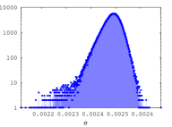
Figure 9: Counting histograms ($y$, blue + red) for the values of $\mu$ (left), $p$ (center) and $\sigma$ (right, $y$-scales are log-scales). The vertical green segment indicates $\mu=0$ (left) and $p=.5$ (center). The red part displays the upper $99\%$ percentile for $|\mu|$ (left) and upper $99.9\%$ percentile for $p$ (center).

We have analyzed the signals of 799 (one gene was missing in our data, out of the 800 tagged in the original paper) sentinels of the yeast cell cycle (YCC) from Spellman et al. (1998), for a total of $\approx$13,600 data points. Figure 9 presents the counting histograms for $\mu$ and $p$ found among all inferred arcs. Let us denote as strong arcs arcs that jointly belong to the red areas of both curves (meaning that both $p$ is in top 99.9$\%$ quantile and $|\mu|$ in top 99$\%$ quantile). We remark that the scale for $\sigma$ is roughly in the tenth of that for $\mu$, so that for strong arcs, distributions with $|\mu|$ in its top 99$\%$ quantile can be considered encoding non-void arc connection (even when small in an absolute scale). We also notice that the distribution in $p$ admits relatively large values ($\approx 0.7$), so that its top $99.9\%$ percentile can be encoding arc probability strictly larger than $1/2$.

G1(P)	FKS1, CLN3, CDC47, RAD54, PCL2, MNN1, RAD53, CLB5	8/16
G1/S	DPB2, CDC2, PRI2, POL12, CDC9, CDC45, CDC21, RNR1, CLB6, POL1, MSH2, RAD27, ASF1,
	POL30, RFA2, PMS1, MST1, RFA1, MSH6, SPC42, CLN2, PCL1, RFA3	23/28
S	MCD1, HTA2, SWE1, HTB1, KAR3, HSL1, HHF2, HHT1, HTB2, CIK1, CLB4	11/17
G2	CLB1, CLB2, BUD8, CDC5	4/4
G2/M	SWI5, CWP1, CHS2, FAR1, DBF2, MOB1, ACE2, CDC6	8/9
M(P)	CDC20	1/2
M(M)	TEC1, RAD51, NUM1	3/4
M(A)	TIP1, SWI4, KIN3, ASF2, ASH1, SIC1, PCL9, EGT2, SED1	9/15
M(T)	$\emptyset$	0/1
M/G1	PSA1, RME1, CTS1	3/3
G1	HO	1/4
late G1	$\emptyset$	0/3

Table 1: Genes found in at least one arc with $p$ in top 99.9$\%$ quantile or $|\mu|$ in top 99$\%$ quantile, in the list of 106 documented genes of the cell cycle in Cho et al. (1998); Rowicka et al. (2007), as a function of the phase as defined in Cho et al. (1998) (left). The right column mentions the number of genes retrieved $/$ total number of genes in the original list (for example, all G2 genes appear).

We have analyzed arcs belonging to at least one of these categories ($p$ is in top 99.9$\%$ quantile or $|\mu|$ in top 99$\%$ quantile), the intersection of both representing strong arcs. Intuitively, this top list should contain most of the (much shorter) "A-lists" of cell-cycle genes as recorded in the litterature. One of these lists (Cho et al., 1998) has been curated and can be retrieved from (Rowicka et al., 2007, Table 4 SI). It contains 106 genes. Table 1 gives the genes we retrieve, meaning that at least one significant arc appear for each of them ($p$ is in top 99.9$\%$ quantile or $|\mu|$ in top 99$\%$ quantile). The values given in the Table allow to concluce that almost $68\%$ of the 106 genes are retrieved as having at least one significant arc. Since the total number of genes with strong arcs we retrieve is 177, out of the 799, the probability that the result observed in Table 1 is due to chance is zero up to more than thirty digits. Hence, assuming the list of genes in Table 1 is indeed a most important one, we can conclude in the reliability of our technique for network discovery for this domain.

	M	M/G1	G1	S	G2
M	18	4	7	3	6
M/G1	5	7	3	0	1
G1	5	4	23	1	0
S	2	0	0	2	1
G2	4	1	0	0	0

Table 2: Distribution of strong arcs ($p$ in top 99.9$\%$ quantile, $|\mu|$ in top 99$\%$ quantile) with respect to phases in the YCC. Each entry has been rounded to the nearest integer for readability.

Figure 10: Distribution of strong arcs ($p$ in top 99.9$\%$ quantile, $|\mu|$ in top 99$\%$ quantile) with respect to phases in the YCC (clockwise), displayed as follows: thick plain $\geq 8\%$, plain $\in[4\%,8\%)$, dashed $\in(2\%,4\%)$. Reference values in Table 2.

As a next step, Table 2 presents the breakdown for the relative distribution of strong arcs in the YCC as a function of the YCC phase, using as reference the original one from Spellman et al. (1998), collapsing the vertices in their respective phase of the YCC to obtain a concise graph of within and between phase dependences (Figure 10 gives a schematic view of the most significant part of the distribution — arcs between different genes of the same YCC phase create the loops observed). We can draw two conclusions: (i) the graph of dependences between phases is not symmetric. Furthermore, (ii) M and G1 appear as the phases which concentrate more than half of the strong arcs, which should be expected given the known regulatory importance in these two phases (Spellman et al., 1998).

	Gene	Phase	out/in-degree ratio
in-degree $<$ out-degree	ASH1	M/G1	5.0
	YIL158W	M	3.0
	MSH6	G1	3.0
	SWI5	M	3.0
	RAD53	G1	3.0
	YNR009W	S	2.5
	MET3	G2	2.3333333333333335
	YOX1	G1	2.0
	SVS1	G1	2.0
	YOL007C	G1	2.0
	CDC20	M	2.0
	YKR041W	G2	2.0
	CDC5	M	2.0
	MET28	S	2.0
	YML034W	M	2.0
	SMC3	G1	2.0
	HHO1	S	2.0
	YDL039C	M	2.0
	RAD27	G1	2.0
	FAR1	M	2.0
	DIP5	M	1.75
	YPL267W	G1	1.6
	CDC45	G1	1.5
	RNR1	G1	1.5
	PCL9	M/G1	1.5
	LEE1	S	1.5
	YOR314W	M	1.5
	YIL025C	G1	1.4444444444444444
	AGP1	G2	1.3333333333333333
	CWP1	G2	1.3333333333333333
	ALD6	M	1.2
	YOL132W	M	1.1666666666666667
	YNR067C	M/G1	1.0666666666666667
in-degree $=$ out-degree	YNL078W	M/G1	1.0
	YCL013W	G2	1.0
	RME1	G1	1.0
	CLB1	M	1.0
	RPI1	M	1.0
	YIL141W	G1	1.0
	BUD4	M	1.0
	YLR235C	G1	1.0
	YOR315W	M	1.0
	YER124C	G1	1.0
	YPR156C	M	1.0
	YGL028C	G1	1.0
	BUD3	G2	1.0
	STE3	M/G1	1.0
	HST3	M	1.0
	ALK1	M	1.0
	CHS2	M	1.0
	YLL061W	S	1.0
	YFR027W	G1	1.0
	LAP4	G1	1.0
	YNL173C	M/G1	1.0
	YML033W	M	1.0
	SEO1	S	1.0
	YOR264W	M/G1	1.0
	NUF2	M	1.0
	YOR263C	M/G1	1.0
	YBR070C	G1	1.0
	YNL300W	G1	1.0
	YPR045C	M	1.0
	YOR248W	G1	1.0
	MYO1	M	1.0
	RLF2	G1	1.0
in-degree $>$ out-degree	YOL101C	M/G1	0.9444444444444444
	YDR355C	S	0.8
	HTB2	S	0.75
	YRO2	M	0.7142857142857143
	YDR380W	M	0.6666666666666666
	FET3	M	0.6666666666666666
	YDL163W	G1	0.6666666666666666
	CLB6	G1	0.6666666666666666
	ECM23	G2	0.6666666666666666
	YBR089W	G1	0.6666666666666666
	YGR221C	G1	0.6666666666666666
	YDL037C	M	0.6
	MF(ALPHA)2	G1	0.6
	YLR183C	G1	0.5714285714285714
	PDR12	M	0.5555555555555556
	YER150W	M/G1	0.5555555555555556
	POL1	G1	0.5
	YHR143W	G1	0.5
	SPS4	M	0.5
	PCL1	G1	0.5
	YGL184C	S	0.5
	EGT2	M/G1	0.5
	CTS1	G1	0.5
	YDR149C	G2	0.5
	GAP1	G2	0.5
	HO	G1	0.5
	WSC4	M	0.4673913043478261
	SPO16	G1	0.46153846153846156
	YMR032W	M	0.4
	YGP1	M/G1	0.4
	SPH1	G1	0.3333333333333333
	YCL022C	G1	0.3333333333333333
	YCLX09W	G2	0.3333333333333333
	PIR1	M/G1	0.25
	ARO9	M	0.16666666666666666

Table 3: Imbalancedness of the network: genes in decreasing ratio out-degree/in-degree, computed using strong arcs ($p$ in top 99.9$\%$ quantile, $|\mu|$ in top 99$\%$ quantile). Only those with $>0$ out-degree and in-degree are shown. A star (*) indicates reported targets for cell-cycle activators (Simon et al., 2001).

To make more precise in observation (i) that the network is indeed imbalanced, we have computed the ratio out-degree $/$ in-degree for all genes admitting strong edges of both kinds (i.e. with the gene as in- / out- node). Table 3 presents all genes collected. A total of 100 genes is found, the majority of which (68) is imbalanced. We also remark that roughly 80$\%$ of them is associated to M and/or G1 (only 19 are associated to phases S or G2), which is consistent with the findings of Table 2.

Gene	Phase	out-degree
WSC4	M	43
YOL101C	M/G1	17
YNR067C	M/G1	16
YIL025C	G1	13
YDL037C	M	12
YOR264W	M/G1	10
YER124C	G1	10
HO	G1	9
YPL267W	G1	8
YLR183C	G1	8
MET3	G2	7
DIP5	M	7
SEO1	S	7
YOL132W	M	7
ALD6	M	6
YGL028C	G1	6
PCL9	M/G1	6
SPO16	G1	6
YDL039C	M	6
YOL007C	G1	6
YER150W	M/G1	5
YRO2	M	5
PDR12	M	5
PCL1	G1	5
YNR009W	S	5
RME1	G1	5
ASH1	M/G1	5
AGP1	G2	4
GAP1	G2	4
YOR263C	M/G1	4
YNL173C	M/G1	4
CWP1	G2	4
FAR1	M	4
MCD1	G1	4
YOX1	G1	4
YDR355C	S	4
YOR314W	M	3
MSH6	G1	3
SPT21	G1	3
LEE1	S	3
YIL158W	M	3
YLR049C	G1	3
RNR1	G1	3
HTB2	S	3
GLK1	M/G1	3
SWI5	M	3
MF(ALPHA)2	G1	3
CDC45	G1	3
RAD53	G1	3

Table 4: Genes in decreasing out-degree for strong arcs ($p$ in top 99.9$\%$ quantile, $|\mu|$ in top 99$\%$ quantile). Only those with out-degree $\geq 3$ are shown.

Gene	Phase	in-degree
WSC4	M	92
YDL037C	M	20
HO	G1	18
YOL101C	M/G1	18
YNR067C	M/G1	15
YLR183C	G1	14
SPO16	G1	13
YOR264W	M/G1	10
YER124C	G1	10
PCL1	G1	10
YIL025C	G1	9
PDR12	M	9
YER150W	M/G1	9
GAP1	G2	8
SEO1	S	7
YRO2	M	7
ARO9	M	6
SPH1	G1	6
YOL132W	M	6
YGL028C	G1	6
MF(ALPHA)2	G1	5
YMR032W	M	5
ALD6	M	5
YPL267W	G1	5
YGP1	M/G1	5
YDR355C	S	5
RME1	G1	5
YOR263C	M/G1	4
YGL184C	S	4
PCL9	M/G1	4
PIR1	M/G1	4
HTB2	S	4
DIP5	M	4
YNL173C	M/G1	4
SPS4	M	4
YCL022C	G1	3
YOL007C	G1	3
MET3	G2	3
YGR221C	G1	3
YDL039C	M	3
CWP1	G2	3
YCLX09W	G2	3
YDR380W	M	3
AGP1	G2	3
CLB6	G1	3
YBR089W	G1	3
FET3	M	3
YDL163W	G1	3
ECM23	G2	3

Table 5: Genes in decreasing in-degree for strong arcs ($p$ in top 99.9$\%$ quantile, $|\mu|$ in top 99$\%$ quantile). Only those with in-degree $\geq 3$ are shown.

To finish with the quantitative analyses, Tables 5 and 4 present the main strong genes in term of in or out degree (genes with in or out-degree $<3$ are not shown). Notice the preeminence of two well known cell-cycle regulated genes, HO and WSC4.

To catch a glimpse at the overall network found from a more qualitative standpoint, we have learned a coordinate system for genes based on a popular manifold learning technique Meila & Shi (2001). Since this technique requires the graph to be symmetric, we have symmetrized the network by taking the max of the $p$-values to weight each edge. Figure 11 presents the results obtained, for the two leading coordinates — excluding the coordinate associated to eigenvalue 1, which encodes the stationary distribution of the Markov chain and is therefore trivial —. It is clear that the first coordinates splits key YCC genes from the rest of the crowd (Cf Tables 5 and 4), also highlighting the importance of WSC4 and strong edges to create the manifold. HO is used to switch mating type and WSC4 is required for maintenance of cell wall integrity Simon et al. (2001).

Interestingly, the most prominent genes belong to a small set of chromosomes (essentially 13, 15, 16). What is quite striking is the fact that SPS4 and SFG1 are in fact neighbors on chromosome XV. It is far beyond the scope of our paper to eventually relate the netork structure and associated causal influence in expression — which we aim to capture — to the proximity in the (physical) loci of genes, but this is eventually worthwhile noticing and exploiting with respect to the already known coexpression of neighboring genes in yeast (Santoni et al., 2013).

Comparison with cpc Last, we have compared our results to those of cpc. Results are shown in Figure 13 for the manifold (compare to Figure 11 for our technique), and in Figure 13 for the distribution of strong arcs found (strong in the case of cpc means $p\geq 0.05$). The graph found is much closer to a complete graph, which is a quite irrealistic observation since cell cycles are extremely inbalanced in terms of importance with respect to regulation. Furthermore, as remarked below in a more quantitative way, it is known that Saccharomyces cerevisiae tends to have a predominant gap phase G1 compared to G2, which is clearly less visible from the cpc results compared to latnet’s results.

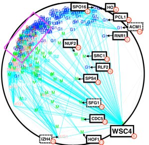
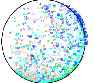
Figure 11: Manifold coordinates learned from the symmetrized $p$-values graph using Meila & Shi (2001), on Klein disk (we chose it to ease reading: the representation is conformal and geodesics are straight lines — WSC4, which is in fact far away from all other genes, does not prevent a visually meaningful display of the other main genes). Segments are strong arcs (arrowheads not represented). Left: Major genes influencing the computation and known to be Cell Cycle Transcriptionally Regulated (CCTR, Rowicka et al. (2007)) are displayed in plain boxes. Chromosomes are shown in red. Right: zoom over the pink area in the left plot, showing few strong edges belong to this area, and therefore strong edges guide the construction of the manifold’s main coordinates.

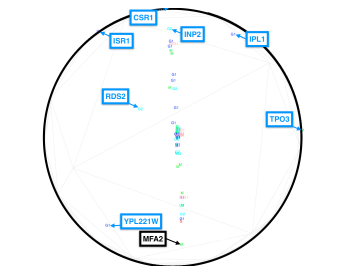
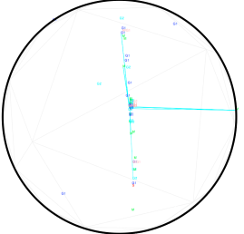
Figure 12: Left: manifold learned from cpc, using the same convention as for latnet. Remark that none of the edges learned by cpc appears, because they are all concentrated inside several blobs that belong to the visible vertical line in the center. Genes displayed in blue are those extremely localed genes that do not belong to the genes in (Rowicka et al., 2007, Table 4 SI). Right: we have substituted the edges learned by cpc by ours, showing that the most important genes in fact belong to the central blob of the picture, therefore not discriminative of the YCC genes.

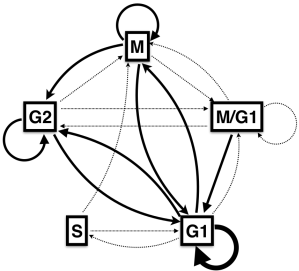
Figure 13: Distribution of strong arcs ($p\geq 0.05$) found by CPC, following Figure 10. Remark that the figure fails to carry the importance of phases M and G1, as Figure 10 for latnet — in particular, phase M roughly carries the same weights distribution as phase G2, which does not conform to observations (G2 is not even mandatory for the YCC while M obviously is).

10.4 Analysis of the complete yeast genome

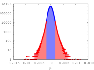
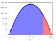
Figure 14: Counting histograms ($y$, blue + red) for the values of $\mu$ (left), $p$ (center) and $\sigma$ (right, $y$-scales are log-scales). Conventions follow Figure 9. A tiny fraction ($<1\text{\textperthousand}$) of arcs found have $p$ or $\sigma$ close to zero; they are not shown to save readability.

We have analyzed the complete set of 6178 genes (representing now $100,000+$ data points) in the yeast genome data Spellman et al. (1998). Not that this time, this represents a maximum of more than 38 millions arcs in total in the network.

Table 6 presents the breakdown in percentages between YCC genes and non-YCC genes. Clearly, the graph is heavily non symmetric: while roughly 11$\%$ of strong arcs come from outside of the YCC to inside the YCC, more than 25$\%$ of these strong arcs come from inside the YCC to outside the YCC. The largest percentage of arcs between YCC - nonYCC is obtained from G1 onto the non YCC genes ($>10\%$), which seems to be plausible, since G1 is a gap phase involving a lot of interactions with the environment, testing for nutrient supply and growth availability. Interestingly, the strong arcs are recalibrated to take into account the complete set of genes (strong arcs are defined with respect to quantiles in data), yet the relative proportions in the YCC still denote the predominance of M and G1, and the very small percentage of strong arcs for phases S and G2. We notice that the predominance of phase G1 compared to G2 is in perfect accordance with the fact that Spellman et al. (1998) picked the yeast Saccharomyces cerevisiae which is indeed known to possess long G1 phases (compared to e.g. Saccharomyces pombe).

Finally, Figure 15 displays the manifold obtained for the complete genome. We represent only a corner of the manifold of 6K+ genes, which displays this time the importance of other YCC genes, including in particular YPR204W. This comes at no surprise: this gene codes for a DNA helicase, a motor protein tht separates DNA strands. DNA helicases are involved in a number of processes and not just the YCC. We do not show strong arcs in the picture, but it is worthwhile remarking that the relative predominance of the most prevalent YCC genes is still here, in the whole genome analysis: WSC4, SPO16 and SLD2 are in the top-5 of out-degree measures with strong arcs.

	M	M/G1	G1	S	G2	N
M	0.6	$\epsilon$	1.2	$\epsilon$	$\epsilon$	2.1
M/G1	$\epsilon$	$\epsilon$	0.2	$\epsilon$	$\epsilon$	1.4
G1	1.0	$\epsilon$	1.0	0.2	$\epsilon$	4.5
S	0.2	$\epsilon$	0.2	$\epsilon$	0.2	2.0
G2	0.2	$\epsilon$	0.2	$\epsilon$	$\epsilon$	1.0
N	6.6	3.5	10.3	2.3	2.9	58.5

Table 6: Distribution of strong arcs ($p$ in top 99.9$\%$ quantile, $|\mu|$ in top 99$\%$ quantile) for the complete genome of the yeast, including the breakdown for the YCC phases (see e.g. Table 2). "$\epsilon$" means $<0.1\%$ and "N" stands for "None" (Gene not in the sentinels of the YCC").

Figure 15: manifold obtained for latnet in the whole yeast genome, conventions follow Figure 11 (strong arcs not displayed for readability).

10.5 Sydney property prices data

We set the discrimination threshold for each method so that on average each method finds 17-19 edges in the network ($p_{ij}=0.597$ for latnet; $p$-value=$0.015$ for pc; $p$-value=$0.012$ for cpc; $p$-value=$10^{-7}$ for iamb; partial correlation$=0.5$ for pw-lingam). Figures 16,17,18,20,19 show the results of latnet, cpc, pc  pw-lingam and iamb algorithms on Sydney property price data. Suburbs were ranked geographically according to their latitude and longitude coordinates, and their locations in the graphs are assigned according to their ranks. We used the ranks instead of actual coordinates of the suburbs in order to be able to better visualize connections in the inner ring. Each panel in the graphs shows the results for a certain period of time, indicated by the label above the panel. Suburbs in Sydney are divided into four groups according to their locations: inner ring (red points), middle ring (green points), outer ring (blue points), and Greater Metropolitan Region (GMR; yellow points).

Data is downloaded from:
http://www.housing.nsw.gov.au/about-us/reports-plans-and-papers/rent-and-sales-reports/back-issues/issue-111

Figure 16: Associations between median house prices in different suburbs discovered by latnet

.

Figure 17: Associations between median house prices in different suburbs discovered by cpc

.

Figure 18: Associations between median house prices in different suburbs discovered by pc

.

Figure 19: Associations between median house prices in different suburbs discovered by pw-lingam

.

Figure 20: Associations between median house prices in different suburbs discovered by iamb

.

References

- Abramowitz & Stegun (1964) Abramowitz, M. and Stegun, I.-A. Handbook of Mathematical Functions with Formulas, Graphs, and Mathematical Tables. U. S. Government Printing Office, 1964.
- Bollen (1989) Bollen, K.-A. Structural equations with latent variables. John Wiley & Sons, 1989.
- Bonilla et al. (2008) Bonilla, E.-V., Chai, K.-M. A, and Williams, C.-K.-I. Multi-task Gaussian process prediction. In NIPS, 2008.
-
Campion (2011)
Campion, Vikki.
http://www.dailytelegraph.com.au/
archive/money/property-prices-in-sydneys-traditional-blue-collar-suburbs-are-booming-with-cabramatta-best-performing-residex-reports/news-story/6971cf79862fdf4f2b3fea3cf2917b5f, 2011. - Chickering (2002) Chickering, D.-M. Optimal structure identification with greedy search. Journal of machine learning research, 3(Nov):507–554, 2002.
- Cho et al. (1998) Cho, R.-J., Campbell, M.-J., Winzeler, E.-A., Steinmetz, L., Conway, A., Wodicka, L., Wolfsberg, T.-G., Gabrielian, A.-E., Landsman, D., Lockhart, D.-J., and Davis, W. A genome-wide transcriptional analysis of the mitotic cell cycle. Molecular Cell, 2:65–73, 1998.
- Hoyer et al. (2009) Hoyer, P.-O., Janzing, D., Mooij, J.-M., Peters, J., and Schölkopf, B. Nonlinear causal discovery with additive noise models. In NIPS, 2009.
- Hyvärinen & Smith (2013) Hyvärinen, A. and Smith, S.-M. Pairwise likelihood ratios for estimation of non-Gaussian structural equation models. JMLR, 14:111–152, 2013.
- Jang et al. (2016) Jang, E., Gu, S., and Poole, B. Categorical reparameterization with gumbel-softmax. arXiv:1611.01144, 2016.
- Kalisch et al. (2012) Kalisch, M., Mächler, M., Colombo, D., Maathuis, M.-H., and Bühlmann, P. Causal inference using graphical models with the R package pcalg. Journal of Statistical Software, 47(11):1–26, 2012.
- Kingma & Ba (2014) Kingma, D.-P. and Ba, J. Adam: A Method for Stochastic Optimization. arXiv:1412.6980, 2014.
- Kingma & Welling (2014) Kingma, D.P. and Welling, M. Auto-Encoding Variational Bayes. In The International Conference on Learning Representations (ICLR), 2014.
- Koyejo & Ghosh (2013) Koyejo, O. and Ghosh, J. Constrained bayesian inference for low rank multitask learning. In UAI, 2013.
- Lawrence (2005) Lawrence, N. Probabilistic non-linear principal component analysis with Gaussian process latent variable models. JMLR, 6:1783–1816, 2005.
- Linderman & Adams (2014) Linderman, S.-W. and Adams, R.-P. Discovering Latent Network Structure in Point Process Data. In ICML, 2014.
- Maddison et al. (2016) Maddison, C.-J., Mnih, A., and Teh, Y.-W. The Concrete Distribution: A Continuous Relaxation of Discrete Random Variables. arXiv:1611.00712, 2016.
- Marco (2010) Marco, S. Learning Bayesian networks with the bnlearn R package. Journal of Statistical Software, 35(3), 2010.
- Meek (1997) Meek, C. Graphical Models: Selecting causal and statistical models. PhD thesis, PhD thesis, Carnegie Mellon University, 1997.
- Meila & Shi (2001) Meila, M. and Shi, J. Learning segmentation by random walks. In NIPS, volume 14, 2001.
- Pearl (2000) Pearl, J. Causality: Models, Reasoning, and Inference. Cambridge University Press, New York, NY, USA, 2000. ISBN 0-521-77362-8.
- Peters et al. (2014) Peters, J., Mooij, J.-M., Janzing, D., and Schölkopf, B. Causal discovery with continuous additive noise models. JMLR, 15(1):2009–2053, 2014.
- Rakitsch et al. (2013) Rakitsch, B., Lippert, C., Borgwardt, K., and Stegle, O. It is all in the noise: Efficient multi-task Gaussian process inference with structured residuals. In NIPS, 2013.
- Ramse et al. (2006) Ramse, J, Zhang, J., and Spirtes, P. Adjacency-faithfulness and conservative causal inference. In Uncertainty in Artificial Intelligence (UAI), 2006.
- Rasmussen & Williams (2005) Rasmussen, C.-E. and Williams, C.-K.-I. Gaussian Processes for Machine Learning (Adaptive Computation and Machine Learning). The MIT Press, 2005. ISBN 026218253X.
- Rezende et al. (2014) Rezende, D.-J., Mohamed, S., and Wierstra, D. Stochastic backpropagation and approximate inference in deep generative models. In ICML, pp. 1278–1286, 2014.
- Rowicka et al. (2007) Rowicka, M., Kudlicki, A., Tu, B.-P., and Otwinowski, Z. High-resolution timing of cell cycle-regulated gene expression. PNAS, 104(43):16892–16897, 2007.
- Santoni et al. (2013) Santoni, D., Castiglione, F., and Paci, P. Identifying correlations between chromosomal proximity of genes and distance of their products in protein-protein interaction networks of yeast. PLoS ONE, 8, 2013.
- Shimizu et al. (2006) Shimizu, S., Hoyer, P.-O., Hyvärinen, A., and Kerminen, A. A linear non-Gaussian acyclic model for causal discovery. JMLR, 7:2003–2030, 2006.
- Shimizu et al. (2011) Shimizu, S., Inazumi, T., Sogawa, Y., Hyvärinen, A., Kawahara, Y., Washio, T., Hoyer, P.-O., and Bollen, K. DirectLiNGAM: A direct method for learning a linear non-gaussian structural equation model. JMLR, 12:1225–1248, 2011.
- Simon et al. (2001) Simon, I., Barnett, J., Hannett, N., Harbison, C.-T., Rinaldi, N.-J., Volkert, T.-L., Wyrick, J.-J., Zeitlinger, J., Gifford, D.-K., Jaakkola, T.-S., and Young, R.-A. Serial regulation of transcriptional regulators in the yeast cell cycle. Cell, 106:697–708, 2001.
- Smith et al. (2011) Smith, S.-M., Miller, K.-L., Salimi-Khorshidi, G., Webster, M., Beckmann, C.-F., Nichols, T.-E., Ramsey, J.-D., and Woolrich, M.-W. Network modelling methods for FMRI. NeuroImage, 54(2):875–891, 2011.
- Spellman et al. (1998) Spellman, P.-T., Sherlock, G., Zhang, M.-Q., Iyer, V.-R., Anders, K., Eisen, M.-B., Brown, P.-O., Botstein, D., and Futcher, B. Comprehensive identification of cell cycle-regulated genes of the yeast Saccharomyces cerevisiae by microarray hybridization. Molecular Biology of the Cell, 9:3273–3297, 1998.
- Spirtes et al. (2000) Spirtes, P., Glymour, C.-N., and Scheines, R. Causation, prediction, and search. MIT press, 2000.
- Tao (2008) Tao, T. Singularity and determinant of random matrices, 2008. Lewis Memorial Lecture.
- Tsagris et al. (2014) Tsagris, M., Beneki, C., and Hassani, H. On the folded normal distribution. Mathematics, 2:12–28, 2014.
- Tsamardinos et al. (2003) Tsamardinos, I., Aliferis, C.-F., Statnikov, A. R, and Statnikov, E. Algorithms for Large Scale Markov Blanket Discovery. In FLAIRS, volume 2, 2003.
- Vu (2014) Vu, V.-H. Modern Aspects of Random Matrix Theory. Proceedings of Symposia in Applied Mathematics. American Mathematical Society, 2014.
- Wilson & Ghahramani (2010) Wilson, A.-G. and Ghahramani, Z. Generalised wishart processes. In UAI, 2010.
- Zhang et al. (2010) Zhang, K., Schölkopf, B., and Janzing, D. Invariant Gaussian Process Latent Variable Models and Application in Causal Discovery. In UAI, 2010.