Multidimensional Vlasov–Poisson Simulations with High-order Monotonicity- and Positivity-preserving Schemes

Abstract

We develop new numerical schemes for Vlasov–Poisson equations with high-order accuracy. Our methods are based on a spatially monotonicity-preserving (MP) scheme and are modified suitably so that positivity of the distribution function is also preserved. We adopt an efficient semi-Lagrangian time integration scheme that is more accurate and computationally less expensive than the three-stage TVD Runge-Kutta integration. We apply our spatially fifth- and seventh-order schemes to a suite of simulations of collisionless self-gravitating systems and electrostatic plasma simulations, including linear and nonlinear Landau damping in one dimension and Vlasov–Poisson simulations in a six-dimensional phase space. The high-order schemes achieve a significantly improved accuracy in comparison with the third-order positive-flux-conserved scheme adopted in our previous study. With the semi-Lagrangian time integration, the computational cost of our high-order schemes does not significantly increase, but remains roughly the same as that of the third-order scheme. Vlasov–Poisson simulations on $128^{3}\times 128^{3}$ mesh grids have been successfully performed on a massively parallel computer.

1 Introduction

Numerical simulations of collisionless self-gravitating systems are one of the indispensable tools in the study of galaxies, galaxy clusters, and the large-scale structure of the universe. Gravitational $N$-body simulations have been widely adopted, and significant scientific achievements have been made for the past four decades. Particles in $N$-body simulations represent the structure of the distribution function in the phase space in a statistical manner. Similarly, particle-in-cell (PIC) simulations (Birdsall & Langdon, 1991) are widely used for studying the dynamics of an astrophysical plasma such as particle acceleration in collisionless shock waves (Matsumoto et al., 2015) and magnetic reconnection (Fujimoto, 2014).

Particle-based $N$-body simulations have several shortcomings, most notably the intrinsic shot noise in the physical quantities such as mass density and velocity field. The discreteness of the mass distribution sampled by a finite number of point mass elements (particles) affects the gravitational dynamics considerably in regions with a small number of particles, in other words, where the phase space density is low. For example, gravitational $N$-body simulations cannot treat collisionless damping of density fluctuations and the two-stream instability in a fluid/plasma with a large velocity dispersion because of poor sampling of particles in the velocity space. Interestingly, physically equivalent situations are observed in PIC simulations (Kates-Harbeck et al., 2016). In PIC simulations, the spacing of grids in the physical space, on which electric and magnetic fields are calculated by solving the Maxwell equations, is constrained not to be larger than the Debye length. Hence, the simulation volume is also restricted for a given number of grids.

To overcome these shortcomings, a number of alternative methods to the $N$-body approach have been proposed. Hernquist & Ostriker (1992) and Hozumi (1997) use the self-consistent field (SCF) method, in which particles move on trajectories on a smooth gravitational potential computed by a basis-function expansion of the density field and gravitational potential. Unlike in conventional $N$-body simulations, particle motions do not suffer from numerical effects owing to discrete gravitational potential. However, a drawback or complication of the SCF method is that the basis functions need to be suitably chosen for a given configuration of the self-gravitating systems.

Abel et al. (2012), Shandarin et al. (2012), and Hahn et al. (2013) develop a novel method to simulate cosmic structure formation by following the motion of dark matter “sheets” in the phase space volume, while retaining the smooth, continuous structure. The method suppresses significantly the artificial discreteness effects in $N$-body simulations such as a spurious filament fragmentation. The method, however, can only be applied to “cold” matter with sufficiently small velocity dispersions compared with its bulk velocity. Vorobyov & Theis (2006) and Mitchell et al. (2013) solve moment equations of the collisionless Boltzmann equation in a finite-volume manner by adopting a certain closure relation. The closure relation needs to be chosen in a problem-dependent manner, and often the validity of the adopted relation remains unclear or its applicability is limited.

A straightforward method to simulate a collisionless plasma or a self-gravitating system is directly solving the collisionless Boltzmann equation, or the Vlasov equation. Such an approach was originally explored by Janin (1971) and Fujiwara (1981) for one-dimensional self-gravitating systems and by Nishida et al. (1981) for two-dimensional stellar disks. It is found to be better in following kinetic phenomena such as collisionless damping and two-stream instability than conventional $N$-body simulations.

The Vlasov–Poisson and Vlasov–Maxwell equations are solved to simulate the dynamics of electrostatic and magnetized plasma, respectively. An important advantage of this approach is that there is no constraint on the mesh spacing, unlike in PIC simulations. In principle, direct Vlasov simulations enable us to simulate the kinematics of an astrophysical plasma with a wide dynamic range, which cannot be easily achieved with PIC simulations.

Despite of its versatile nature, the Vlasov simulations have been applied only to problems in one or two spatial dimensions. Solving the Vlasov equation with three spatial dimensions, i.e., in a six-dimensional phase space, requires an extremely large amount of memory. Yoshikawa et al. (2013) successfully perform Vlasov–Poisson simulations of self-gravitating systems in six-dimensional phase space, achieving high accuracies in mass and energy conservation. Unfortunately, the number of grids is still limited by the amount of available memory rather than the computational cost. With currently available computers, it is not realistic to achieve a significant increase in spatial (and velocity) resolution by simply increasing the number of mesh grids. Clearly, developing high-order schemes is necessary to effectively improve the spatial resolution for a given number of mesh grids. In the present paper, we develop and test new numerical schemes for solving the Vlasov equation based on the fifth- and seventh-order monotonicity-preserving (MP) schemes (Suresh & Huynh, 1997). We improve the schemes suitably so that the positivity of the distribution function is ensured. We run a suite of test simulations and compare the results with those obtained by the spatially third-order positive-flux-conservative (PFC) scheme (Filbet et al., 2001) adopted in our previous work (Yoshikawa et al., 2013, hereafter YYU13).

The rest of the paper is organized as follows. In section 2, we describe our new numerical schemes to solve the Vlasov equation in higher-order accuracy in detail. Section 3 is devoted to presenting several test calculations to show the technical advantage of our approach over the previous methods. We address the computational costs of our schemes in section 4. Finally, in section 5, we summarize our results and present our future prospects.

2 Vlasov–Poisson Simulation

We follow the time evolution of the distribution function $f(\textbf{{x}},\textbf{{v}},t)$ according to the following Vlasov (collisionless Boltzmann) equation:

$$\frac{\partial f}{\partial t}+\frac{d\textbf{{x}}}{dt}\cdot\frac{\partial f}{\partial\textbf{{x}}}+\frac{d\textbf{{v}}}{dt}\cdot\frac{\partial f}{\partial\textbf{{v}}}=0,$$ (1)

where $\textbf{{x}}=(x_{1},x_{2},x_{3})=(x,y,z)$ and $\textbf{{v}}=(v_{1},v_{2},v_{3})=(v_{x},v_{y},v_{z})$ are the Cartesian spatial and velocity coordinates, respectively. For self-gravitating systems, it gives the Vlasov–Poisson equation is given as

$$\frac{\partial f}{\partial t}+\textbf{{v}}\cdot\frac{\partial f}{\partial\textbf{{x}}}-\frac{\partial\phi}{\partial\textbf{{x}}}\cdot\frac{\partial f}{\partial\textbf{{v}}}=0,$$ (2)

where $\phi$ is the gravitational potential satisfying the Poisson equation

$$\nabla^{2}\phi=4\pi G\rho=4\pi G\int f\,{\rm d}^{3}\textbf{{v}},$$ (3)

where $G$ is the gravitational constant and $\rho$ is the mass density. Throughout the present paper, the distribution function is normalized such that its integration over velocity space yields the mass density. We discretize the distribution function $f(\textbf{{x}},\textbf{{v}},t)$ in the same manner as in YYU13; we employ a uniform Cartesian mesh in both the physical configuration space and in the velocity (momentum) space.

2.1 Advection Solver

The Vlasov Equation (2) can be broken down into six one-dimensional advection equations along each dimension of the phase space: three for advection in the physical space

$$\frac{\partial f}{\partial t}+v_{i}\frac{\partial f}{\partial x_{i}}=0\,\,\,\,\,\,\,\,\,\,\,(i=1,2,3),$$ (4)

and another three in the velocity space

$$\frac{\partial f}{\partial t}-\frac{\partial\phi}{\partial x_{i}}\frac{\partial f}{\partial v_{i}}=0\,\,\,\,\,\,\,\,\,\,\,(i=1,2,3).$$ (5)

We solve these six equations sequentially. The gravitational potential $\phi$ in Equation (5) is updated after advection Equation (4) in the physical space is solved and the mass density distribution in the physical space is updated. Clearly, an accurate numerical scheme for a one-dimensional advection scheme is a crucial ingredient of our Vlasov solver.

Let us consider a numerical scheme of the following advection equation

$$\frac{\partial f(x,t)}{\partial t}+c\frac{\partial f(x,t)}{\partial x}=0,$$ (6)

on a one-dimensional uniform mesh grid. In a finite-volume manner, we define an averaged value of $f(x,t)$ over the $i$th grid centered at $x=x_{i}$ with the interval of $\Delta x$ at a time $t=t^{n}$ as

$$f^{n}_{i}=\frac{1}{\Delta x}\int_{x_{i-1/2}}^{x_{i+1/2}}f(x,t^{n})\,{\rm d}x,$$ (7)

where $x_{i\pm 1/2}=x_{i}\pm\Delta x/2$ are the coordinates of the boundaries of the $i$th mesh grid. Without loss of generality, we can restrict ourselves to the case with a positive advection velocity $c>0$.

Physical and mathematical considerations impose the following requirements on numerical solutions of the advection equation: (i) Monotonicity—since the solution of the advection Equation (6) preserves monotonicity, so should its numerical solution. (ii) Positivity—the distribution function must be positive by definition, and thus the numerical solution should be non-negative. Note that monotonicity is not sufficient to ensure positivity of the numerical solution.

2.1.1 MP Schemes with the Positivity-preserving Limiter

We first present the spatially fifth-order scheme for the advection Equation (6) based on the MP5 scheme of Suresh & Huynh (1997), in which the value of $f(x,t)$ at the interface between the $(i-1)$th and $i$th mesh grids is reconstructed with five stencils $f^{n}_{i-3}$, $f^{n}_{i-2}$, $f^{n}_{i-1}$, $f^{n}_{i}$, and $f^{n}_{i+1}$ as

$$f^{\rm int,5}_{i-1/2}=(2f_{i-3}-13f_{i-2}+47f_{i-1}+27f_{i}-3f_{i+1})/60.$$ (8)

In order to ensure monotonicity of the numerical solution, we impose the constraint

$$\bar{f}_{i-1/2}={\rm MP}(f^{\rm int,5}_{i-1/2},f_{i-3},f_{i-2},f_{i-1}.f_{i},f_{i+1})$$ (9)

The detailed prescriptions of the constraints are given in Appendix A. The MP5 scheme adopts the three-stage TVD Runge-Kutta (TVD–RK) time integration as

$$f^{(1)}_{i} = f^{n}_{i}-\nu L_{i}(f^{n})$$

$$f^{(2)}_{i} = \frac{3}{4}f^{n}_{i}+\frac{1}{4}\left(f_{i}^{(1)}-\nu L_{i}(f^{(1)})\right)$$ (10)

$$f^{n+1}_{i} = \frac{1}{3}f^{n}_{i}+\frac{2}{3}\left(f_{i}^{(2)}-\nu L_{i}(f^{(2)})\right),$$

where $\nu=c\Delta t/\Delta x$ is the CFL number and the operator $L_{i}(f)$ is defined as

$$L_{i}(f)=\bar{f}_{i+1/2}-\bar{f}_{i-1/2}.$$ (11)

Hereafter, this scheme is referred to as RK–MP5.

As already noted above, the MP scheme does not ensure positivity of the numerical solution. We thus introduce a positivity-preserving (PP) limiter based on the method proposed by Hu et al. (2013). By denoting $U_{i}^{+}=f_{i}^{n}-2\nu\bar{f}^{n}_{i+1/2}$ and $U_{i}^{-}=f^{n}_{i}+2\nu\bar{f}^{n}_{i-1/2}$, the single-stage Eulerian time integration can be written as

$$f^{(1)}_{i} = f^{n}_{i}-\nu(\bar{f}^{n}_{i+1/2}-\bar{f}^{n}_{i-1/2})$$ (12)

$$= \frac{1}{2}\left(f^{n}_{i}-2\nu\bar{f}^{n}_{i+1/2}\right)+\frac{1}{2}\left(f^{n}_{i}+2\nu\bar{f}^{n}_{i-1/2}\right)$$ (13)

$$= \frac{1}{2}U_{i}^{+}+\frac{1}{2}U_{i}^{-}.$$ (14)

Here, we consider a linear combination of the interface value obtained with the MP scheme and that with the spatially first-order upwind scheme as

$$\hat{f}^{n}_{i+1/2}=\theta_{i+1/2}\bar{f}^{n}_{i+1/2}+(1-\theta_{i+1/2})f^{{\rm UP},n}_{i+1/2},$$ (15)

where $f^{{\rm UP},n}_{i+1/2}$ is expressed as

$$f^{{\rm UP},n}_{i+1/2}=\frac{1}{2c}\left[f^{n}_{i}(c+|c|)+f^{n}_{i+1}(c-|c|)\right]=f_{i}^{n},$$ (16)

and $\theta_{i+1/2}$ is a parameter with a condition of $0\leq\theta_{i+1/2}\leq 1$. Note that the spatially first-order upwind scheme preserves positivity of the numerical solution if the CFL condition $\nu\leq 1$ is satisfied. Then, the time integration of the combined interface values (15) can be written as

$$f^{(1)}_{i} = f_{i}^{n}-\nu(\hat{f}^{n}_{i+1/2}-\hat{f}^{n}_{i-1/2})$$ (17)

$$= \frac{1}{2}\left(f^{n}_{i}-2\nu\hat{f}^{n}_{i+1/2}\right)+\frac{1}{2}\left(f^{n}_{i}+2\nu\hat{f}^{n}_{i-1/2}\right)$$ (18)

$$= \frac{1}{2}\left\{\theta_{i+1/2}U^{+}_{i}+(1-\theta_{i+1/2})U^{\rm UP,+}_{i}\right\}+\frac{1}{2}\left\{\theta_{i-1/2}U^{-}_{i}+(1-\theta_{i-1/2})U^{\rm UP,-}_{i}\right\},$$ (19)

where $U_{i}^{\rm UP,+}=f_{i}^{n}-2\nu f^{{\rm UP},n}_{i+1/2}$ and $U_{i}^{\rm UP,-}=f_{i}^{n}+2\nu f^{{\rm UP},n}_{i-1/2}$. Therefore, if both of the two terms on the right-hand side of Equation (19) are positive, $f^{(1)}_{i}$ is also positive. A simple calculation shows that it can be realized by setting the parameter $\theta_{i+1/2}$ as

$$\theta_{i+1/2}=\min(\theta_{i+1/2}^{+},\theta_{i+1/2}^{-}),$$ (20)

where

$$\theta_{i+1/2}^{+}=\left\{\begin{array}[]{ll}\displaystyle\frac{U_{i}^{\rm UP,+}}{U_{i}^{\rm UP,+}-U_{i}^{+}}&\,\,\,\,\mbox{if $U_{i}^{+}<0$}\\ 1&\,\,\,\,\mbox{otherwise}\end{array}\right.$$ (21)

and

$$\theta_{i+1/2}^{-}=\left\{\begin{array}[]{ll}\displaystyle\frac{U_{i+1}^{\rm UP,-}}{U_{i+1}^{\rm UP,-}-U_{i+1}^{-}}&\,\,\,\,\mbox{if $U_{i+1}^{-}<0$}\\ 1&\,\,\,\,\mbox{otherwise.}\end{array}\right.$$ (22)

In addition, the condition of $\theta_{i+1/2}\geq 0$ can be met by setting $U_{i}^{\rm UP,+}\geq 0$ and $U_{i+1}^{\rm UP,-}\geq 0$ as a sufficient condition, which leads to a constraint on the CFL parameter as $\nu\leq 1/2$. Let us denote the above procedures to evaluate the positive interface value (15) as

$$\hat{f}^{n}_{i+1/2}={\rm PP}(\bar{f}^{n}_{i+1/2},f^{n}_{i},f^{n}_{i+1}).$$ (23)

It can be shown that positivity of the numerical solution is preserved even with the three-stage TVD–RK time integration by setting the CFL parameter to $\nu<1/2$. In the following, we call this scheme the RK–MPP5 scheme (MPP for “monotonicity and positivity preserving”).

It is tedious but straightforward to construct the spatially seventh-order schemes, RK–MP7 and RK–MPP7, by simply replacing $f_{i-1/2}^{\rm int,5}$ in Equation (9) with the seventh-order interpolation

$$f_{i-1/2}^{\rm int,7}=(-3f_{i-4}+25f_{i-3}-101f_{i-2}+319f_{i-1}+214f_{i}-38f_{i+1}+4f_{i+2})/420.$$ (24)

2.1.2 Semi-Lagrangian Time Integration

The MP schemes described above adopt the three-stage TVD–RK time integration (10), which needs explicit Euler integration three times per single time step. It can be a source of significant computational cost. To overcome this drawback, we devise an alternative method based on the semi-Lagrangian (SL) time integration.

The averaged value of $f(x,t)$ over the $i$th mesh grid $f^{n+1}_{i}$ at a time of $t^{n+1}=t^{n}+\Delta t$ is written as

$$f^{n+1}_{i}=\frac{1}{\Delta x}\int_{x_{i-1/2}}^{x_{i+1/2}}f(x,t^{n+1})\,{\rm d}x=\frac{1}{\Delta x}\int_{X(t^{n},t^{n+1},x_{i-1/2})}^{X(t^{n},t^{n+1},x_{i+1/2})}f(x,t^{n})\,{\rm d}x,$$ (25)

where $X(t_{1},t_{2},x)$ is the position of the characteristic curve at a time of $t_{1}$ originating from the phase space coordinate $(x,t_{2})$, and for the advection Equation (6), $X(t_{1},t_{2},x)=x-c(t_{2}-t_{1})$; see Figure 1. Denoting

$$\Phi^{n}_{i+1/2}=\frac{1}{c\Delta t}\int_{X(t^{n},t^{n+1},x_{i+1/2})}^{x_{i+1/2}}f(x,t^{n})\,{\rm d}x$$ (26)

and

$$\Phi^{n}_{i-1/2}=\frac{1}{c\Delta t}\int^{x_{i-1/2}}_{X(t^{n},t^{n+1},x_{i-1/2})}f(x,t^{n})\,{\rm d}x,$$ (27)

we can rewrite the Equation (25) in terms of numerical flux as

$$f^{n+1}_{i}=f^{n}_{i}-\nu(\Phi^{n}_{i+1/2}-\Phi^{n}_{i-1/2}).$$ (28)

By interpolating the discrete values of $f^{n}_{j}$, we can compute the numerical fluxes $\Phi_{i+1/2}$ and $\Phi_{i-1/2}$. Actually, the PFC scheme also adopts essentially the same approach. It adopts the third-order reconstruction to interpolate $f^{n}_{j}$ with a slope limiter and suppresses numerical oscillation while preserving positivity of the numerical solutions. For more detailed description of the PFC scheme, see Filbet et al. (2001) and the Appendix of YYU13.

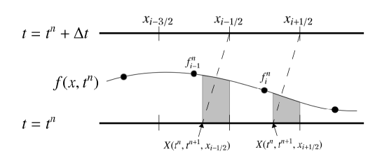
Figure 1: Schematic description of the semi-Lagrangian scheme. Dashed lines starting from $x_{i\pm 1/2}$ are the characteristic curves. The areas of the left and right shaded regions correspond to $\Phi_{i-1/2}$ and $\Phi_{i+1/2}$, respectively.

Our new schemes are based on the conservative semi-Lagrangian (CSL) scheme (Qiu & Christlieb, 2010; Qiu & Shu, 2011), which is originally coupled with a finite-difference scheme but is also applicable to the finite-volume schemes. In the fifth-order CSL scheme, $\Phi^{n}_{i-1/2}$ can be expressed with five stencil values as

$$\Phi^{n}_{i-1/2}=\sum_{j=0}^{4}C_{j}\zeta^{j}$$ (29)

where

$$C_{0}=\frac{f^{n}_{i-3}}{30}-\frac{13}{60}f^{n}_{i-2}+\frac{47}{60}f^{n}_{i-1}+\frac{9}{20}f^{n}_{i}-\frac{f^{n}_{i+1}}{20}$$ (30)

$$C_{1}=-\frac{f^{n}_{i-2}}{24}+\frac{5}{8}f^{n}_{i-1}-\frac{5}{8}f^{n}_{i}+\frac{f^{n}_{i+1}}{24}$$ (31)

$$C_{2}=-\frac{f^{n}_{i-3}}{24}+\frac{f^{n}_{i-2}}{4}-\frac{f^{n}_{i-1}}{3}+\frac{f^{n}_{i}}{12}+\frac{f^{n}_{i+1}}{24}$$ (32)

$$C_{3}=\frac{f^{n}_{i-2}}{24}-\frac{f^{n}_{i-1}}{8}+\frac{f^{n}_{i}}{8}-\frac{f^{n}_{i+1}}{24}$$ (33)

$$C_{4}=\frac{f^{n}_{i-3}}{120}-\frac{f^{n}_{i-2}}{30}+\frac{f^{n}_{i-1}}{20}-\frac{f^{n}_{i}}{30}+\frac{f^{n}_{i+1}}{120}$$ (34)

and

$$\zeta=\frac{c\Delta t}{\Delta x}.$$ (35)

The seventh-order CSL scheme is given by

$$\Phi^{n}_{i-1/2}=\sum_{j=0}^{6}D_{j}\zeta^{j},$$ (36)

where

$$D_{0}=-\frac{f^{n}_{i-4}}{140}+\frac{5}{84}f^{n}_{i-3}-\frac{101}{420}f^{n}_{i-2}+\frac{319}{420}f^{n}_{i-1}+\frac{107}{210}f^{n}_{i}-\frac{19}{210}f^{n}_{i+1}+\frac{f^{n}_{i+2}}{105}$$ (37)

$$D_{1}=\frac{f^{n}_{i-3}}{180}-\frac{5}{72}f^{n}_{i-2}+\frac{49}{72}f^{n}_{i-1}-\frac{49}{72}f^{n}_{i}+\frac{5}{72}f^{n}_{i+1}-\frac{f^{n}_{i+2}}{180}$$ (38)

$$D_{2}=\frac{7}{720}f^{n}_{i-4}-\frac{19}{240}f^{n}_{i-3}+\frac{7}{24}f^{n}_{i-2}-\frac{23}{72}f^{n}_{i-1}+\frac{f^{n}_{i}}{48}+\frac{7}{80}f^{n}_{i+1}-\frac{f^{n}_{i+2}}{90}$$ (39)

$$D_{3}=-\frac{f^{n}_{i-3}}{144}+\frac{11}{144}f^{n}_{i-2}-\frac{7}{36}f^{n}_{i-1}+\frac{7}{36}f^{n}_{i}-\frac{11}{144}f^{n}_{i+1}+\frac{f^{n}_{i+2}}{144}$$ (40)

$$D_{4}=-\frac{f^{n}_{i-4}}{360}+\frac{f^{n}_{i-3}}{48}-\frac{13}{240}f^{n}_{i-2}+\frac{23}{360}f^{n}_{i-1}-\frac{f^{n}_{i}}{30}+\frac{f^{n}_{i+1}}{240}+\frac{f^{n}_{i+2}}{720}$$ (41)

$$D_{5}=\frac{f^{n}_{i-3}}{720}-\frac{f^{n}_{i-2}}{144}+\frac{f^{n}_{i-1}}{72}-\frac{f^{n}_{i}}{72}+\frac{f^{n}_{i+1}}{144}-\frac{f^{n}_{i+2}}{720}$$ (42)

and

$$D_{6}=\frac{f^{n}_{i-4}}{5040}-\frac{f^{n}_{i-3}}{840}+\frac{f^{n}_{i-2}}{336}-\frac{f^{n}_{i-1}}{252}+\frac{f^{n}_{i}}{336}-\frac{f^{n}_{i+1}}{840}+\frac{f^{n}_{i+2}}{5040}.$$ (43)

However, the numerical solution obtained with the CSL scheme does not preserve the monotonicity. Thus, we apply the MP constraint to $\Phi^{n}_{i-1/2}$ and $\Phi^{n}_{i+1/2}$ as

$$\bar{\Phi}^{n}_{i-1/2}={\rm MP}(\Phi^{n}_{i-1/2},f^{n}_{i-3},f^{n}_{i-2},f^{n}_{i-1},f^{n}_{i},f^{n}_{i+1})$$ (44)

and

$$\bar{\Phi}^{n}_{i+1/2}={\rm MP}(\Phi^{n}_{i+1/2},f^{n}_{i-2},f^{n}_{i-1},f^{n}_{i},f^{n}_{i+1},f^{n}_{i+2}).$$ (45)

The numerical solution with the monotonicity preservation at $t=t^{n+1}$ is then computed as

$$f^{n+1}_{i}=f^{n}_{i}-\nu(\bar{\Phi}^{n}_{i+1/2}-\bar{\Phi}^{n}_{i-1/2}),$$ (46)

which is referred to as the SL–MP5 and SL–MP7 schemes (SL for “semi-Lagrangian”) for the fifth- and seventh-order accuracies, respectively.

The PP limiter described in the previous subsection can be applied as

$$\hat{\Phi}^{n}_{i-1/2}={\rm PP}(\bar{\Phi}^{n}_{i-1/2},f^{n}_{i-1},f^{n}_{i})$$ (47)

and

$$\hat{\Phi}^{n}_{i+1/2}={\rm PP}(\bar{\Phi}^{n}_{i+1/2},f^{n}_{i},f^{n}_{i+1}).$$ (48)

Then, the numerical solution at $t^{n+1}$ is given by

$$f^{n+1}_{i}=f^{n}_{i}-\nu(\hat{\Phi}^{n}_{i+1/2}-\hat{\Phi}^{n}_{i-1/2}).$$ (49)

We refer to these schemes as the SL–MPP5 and SL–MPP7 schemes hereafter.

2.2 Poisson Solver

The Poisson Equation (3) is numerically solved with the convolution method (Hockney & Eastwood, 1981) using the fast Fourier transform (FFT). Under periodic boundary conditions, the discrete Fourier transform (DFT) of the gravitational potential $\phi(\textbf{{k}})$ can be written as

$$\hat{\phi}({\textbf{{k}}})=G(\textbf{{k}})\hat{\rho}(\textbf{{k}})$$ (50)

where $\hat{\rho}(\textbf{{k}})$ is the DFT of the density field, $\textbf{{k}}=(k_{x},k_{y},k_{z})$ is the discrete wavenumber vector, and $G(\textbf{{k}})$ is the Fourier-transformed Green function of the discretized Poisson equation. The second-order discretization of the Green function, $G(\textbf{{k}})$, is given by

$$G(\textbf{{k}})=-\frac{\pi G\Delta^{2}}{\displaystyle\sum_{i=x,y,z}\sin^{2}\left(\frac{k_{i}\Delta}{2}\right)}$$ (51)

with $\Delta x=\Delta y=\Delta z=\Delta$. Since we adopt advection solvers with spatially fifth- and seventh-order accuracy, it is reasonable to adopt a Poisson solver with the same or similar order of accuracy, which can be simply constructed by high-order discretization of the Poisson equation. As shown in Appendix C, the DFTs of the Green functions with spatially fourth- and sixth-order accuracy are given by

$$G(\textbf{{k}})=\frac{12\pi G\Delta^{2}}{\displaystyle\sum_{i=x,y,z}\left[\sin^{2}(k_{i}\Delta)-16\sin^{2}\left(\frac{k_{i}\Delta}{2}\right)\right]}$$ (52)

and

$$G(\textbf{{k}})=-\frac{180\pi G\Delta^{2}}{\displaystyle\sum_{i=x,y,z}\left[2\sin^{2}\left(\frac{3k_{i}\Delta}{2}\right)-27\sin^{2}(k_{i}\Delta)+270\sin^{2}\left(\frac{k_{i}\Delta}{2}\right)\right]},$$ (53)

respectively. The gravitational potential $\phi(\textbf{{x}})$ is computed with the inverse DFT of $\hat{\phi}(\textbf{{k}})$.

For isolated boundary conditions, the doubling-up method (Hockney & Eastwood, 1981) is adopted, where the number of mesh grids is doubled for each spatial dimension and the mass density in the extended grid points is zeroed out. The Green function is set up in the real space as

$$G(x,y,z)=\frac{G}{(x^{2}+y^{2}+z^{2})^{1/2}}$$ (54)

and is Fourier-transformed to obtain $\hat{G}(\textbf{{k}})$. Then, the gravitational potential can be calculated in the same manner as in the the periodic boundary condition.

After obtaining the gravitational potential, we compute gravitational forces at each of the spatial grids with the finite-difference approximation (FDA). Again we adopt FDA schemes with the same order of accuracy as that of the gravitational potential calculation. The two-, four- and six-point FDAs are described in Appendix C. In what follows, we adopt the sixth-order calculation of the gravitational forces and potentials irrespective of adopted advection schemes because we are primarily interested in the accuracy of our advection equation solver.

2.3 Parallelization and Domain Decomposition

We parallelize our Vlasov–Poisson solvers by decomposing the six-dimensional phase space into distributed memory spaces. We decompose the computational domain in the phase space in the same manner as YYU13. The physical space is divided into rectangular subdomains along $x$-, $y$-, and $z$-directions, while the velocity space is not decomposed; each spatial point has an entire set of velocity mesh grids. This decomposition is convenient when computing the velocity moments of the distribution function such as the mass density, mean velocities, and velocity dispersions.

In solving the advection equations in the physical space (4) across the decomposed subdomains, the values of the distribution function adjacent to the boundaries of the subdomains are transferred using the Message Passing Interface (MPI). The number of the adjacent mesh grids to be transferred is two for the spatially third-order PFC scheme and three and four for spatially fifth- and seventh-order MP schemes, respectively.

2.4 Time Integration

We advance the distribution function from $t=t^{n}$ to $t^{n+1}$ using the directional splitting method on the order of

$$f(\textbf{{x}},\textbf{{v}},t^{n+1}) = T_{v_{z}}(\Delta t/2)T_{v_{y}}(\Delta t/2)T_{v_{x}}(\Delta t/2)$$ (55)

$$\times T_{x}(\Delta t)T_{y}(\Delta t)T_{z}(\Delta t)$$

$$\times T_{v_{z}}(\Delta t/2)T_{v_{y}}(\Delta t/2)T_{v_{x}}(\Delta t/2)f(\textbf{{x}},\textbf{{v}},t^{n}),$$

where $T_{\ell}(\Delta t)$ denotes an operator for advection along the $\ell$-direction with time step $\Delta t$. It should be noted that the Poisson equation is solved after the advection operations in the physical space ($T_{x}T_{y}T_{z}$) to update the gravitational potential and forces for the updated density field. We adopt the directional splitting method rather than the unsplit method because the former is the combination of one-dimensional advection schemes and hence rigorously assures the monotonicity and the positivity even in the multidimensional problems and also because the latter requires a larger amount of memory space to temporally store the numerical fluxes or the updated distribution function. Furthermore, the unsplit method requires a relatively smaller time step than the directional splitting method to achieve the same level of numerical accuracy. See section 3.1.4 for the comparison of the dimensional splitting and unsplit methods in the two-dimensional advection problems. The temporal accuracy of the directional splitting method is in the second order at best. However, we find that the errors in the numerical solutions presented in the following numerical test are mostly dominated by ones that originate from the spatial discretization, and the spatial resolution is more important than the temporal accuracy in terms of the quality of the numerical solution.

As for time step width, we have several constraints on the CFL parameter. The MP schemes are subject to the constraint with $\nu\leq 1/5$ if the parameter $\alpha$ in the MP scheme is set to $\alpha=4$ (see Appendix A) and the PP limiter requires $\nu\leq 1/2$. As shown in Appendix B, all of our new schemes work well for $3<\alpha$ and $\nu<0.4$. In practice, the condition $\nu=1/(1+\alpha)$ is desirable, and thus we set $\alpha=4$ and $\nu=0.2$ throughout the present paper unless otherwise stated.

We set the time step for integrating the Vlasov equation as

$$\Delta t=\min(\Delta t_{\rm p},\Delta t_{\rm v}),$$ (56)

where $\Delta t_{\rm p}$ and $\Delta t_{\rm v}$ are the time steps for advection equations in physical and velocity space, respectively. $\Delta t_{\rm p}$ is given by

$$\Delta t_{\rm p}=\nu\min\left(\frac{\Delta x}{V_{x}^{\rm max}},\frac{\Delta y}{V_{y}^{\rm max}},\frac{\Delta z}{V_{z}^{\rm max}}\right),$$ (57)

where $\Delta\ell$ denotes the spacing of mesh grids along the $\ell$-direction and $V_{\ell}^{\rm max}$ is the maximum extent of the velocity space along the $v_{\ell}$-direction. Similarly, we compute $\Delta t_{\rm v}$ as

$$\Delta t_{\rm v}=\nu\min_{i}\left(\frac{\Delta v_{x}}{|a_{x,i}|},\frac{\Delta v_{y}}{|a_{y,i}|},\frac{\Delta v_{z}}{|a_{z,i}|}\right),$$ (58)

where $a_{\ell,i}$ is the gravitational acceleration along the $\ell$-direction at the $i$th mesh grids in the physical space and the minimization is taken over all the spatial mesh grids.

3 Test Calculations

In this section, we present the results of several test simulations with our new schemes. The test suite includes simulations of one- and two-dimensional advection and Vlasov–Poisson simulations in two- and six-dimensional phase space.

3.1 Test-1: Advection Equation

As the first of the test suite of our new schemes, we perform numerical simulations of the advection equation. Here, we solve the one- and two-dimensional advection equations. In the one-dimensional tests, we examine the fundamental properties of our new schemes such as monotonicity, positivity, and accuracy. In the two-dimensional tests, we present the applicability of our one-dimensional schemes to multidimensional problems.

The first test run we perform is the one-dimensional advection problem. We solve

$$\frac{\partial f(x,t)}{\partial t}+\frac{\partial f(x,t)}{\partial x}=0$$ (59)

with our new schemes. Since the accuracy of the numerical solutions depends on the shape of $f(x,t)$, we consider three initial conditions and examine critically the numerical solutions.

3.1.1 Test-1a: Rectangular-shaped Function

We configure the rectangular-shaped initial condition given by

$$f(x,t=0)=\left\{\begin{array}[]{lll}1&&0.25\leq x\leq 0.75\\ 0&&{\rm otherwise}\end{array}\right.$$ (60)

in the simulation domain over $0\leq x\leq 1$ and integrate equation (59) using PFC, RK–MPP5, RK–MPP7, SL–MPP5, and SL–MPP7 under the periodic boundary conditions. Figure 3.1.1 shows the numerical solutions at $t=8$ with the number of mesh grids $N_{\rm m}=64$. The numerical solutions with RK–MPP5, SL–MPP5, and SL–MPP7 are less diffusive compared with that of PFC. Note that RK–MPP7 yields undesirable asymmetric features around $x\simeq 0.2$ and $0.7$. Actually these features are persistent irrespective of $N_{\rm m}$ and $\nu$, and are likely caused by the lack of accuracy in the time integration. In order to avoid these features, we would need the fourth- or higher-order TVD–RK integration schemes, which are computationally quite expensive (see § 4). Thus, we exclude RK–MP7 and RK–MPP7 in the rest of our test simulations. Unlike RK–MPP7, SL–MPP7 does not exhibit such features, indicating that the SL time integration method is able to be combined with spatially seventh- or higher-order schemes. We confirm that the spatially ninth-order CSL scheme combined with the SL method works well at least in one-dimensional advection problems. Figure 2 shows the relative error of the numerical solutions to the analytic solution defined as

$$\epsilon_{1{\rm D}}=\frac{\displaystyle\sum_{i=1}^{N_{\rm m}}|f_{i}-f(x_{i},t)|}{\displaystyle\sum_{i=1}^{N_{\rm m}}|f(x_{i},t)|}.$$ (61)

Since there are discontinuities in the initial condition, the numerical fluxes computed with PFC and our new schemes are effectively of the first order, avoiding numerical oscillations. This is why the relative errors scale with the first-order power law.

Test-1a (rectangular-shaped function): profiles of the initially rectangular-shaped function at $t=8$ computed with PFC, RK–MPP5, RK–MPP7, SL–MPP5, and SL–MPP7. $N_{\rm m}$ is set to 64.

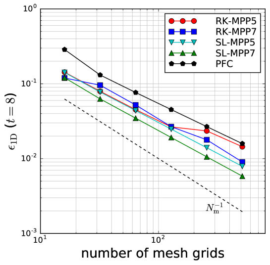
Figure 2: Test-1a (rectangular-shaped function): relative errors of the numerical solutions computed with PFC, RK–MPP5, RK–MPP7, SL–MPP5, and SL–MPP7. A thin dashed line indicates the error scaling proportional to $N_{\rm m}^{-1}$.

3.1.2 Test-1b: Sinusoidal Wave

As a good example of advection of a smooth function, we consider the initial condition given by

$$f(x,t=0)=1+\sin(2\pi x),$$ (62)

in the periodic domain of $0\leq x\leq 1$. Figure 3 shows the relative errors of numerical solutions obtained with RK–MPP5, SL–MPP5, and SL–MPP7 in the left panel and with RK–MP5, SL–MP5, and SL–MP7 without the PP limiter in the right panel as a function of $N_{\rm m}$. For comparison, the result obtained with PFC is also presented in both the panels. The numerical solutions obtained with RK–MPP5 have nearly third-order accuracy for $N_{\rm m}\gtrsim 10^{2}$, whereas those with RK–MP5 have fifth-order accuracy. This is because the PP limiter operates at the minima of numerical solutions at each stage of the TVD–RK time integration and degrades overall accuracy. Contrastingly, the accuracies of the SL schemes are not affected by the PP limiter, i.e., the results of SL–MPP5 and SL–MPP7 show fifth- and seventh-order scaling.

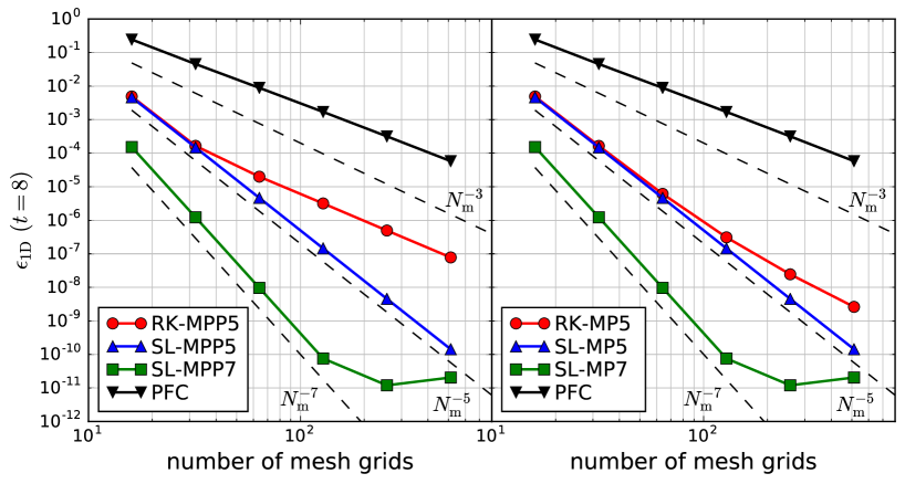
Figure 3: Test-1b (sinusoidal wave): relative errors of the advection of sinusoidal waves computed with schemes with and without the PP limiter in the left and right panels, respectively. Thin dashed lines in each panels indicate the scalings of the numerical errors in the third-, fifth-, and seventh-order accuracies from top to bottom.

3.1.3 Test-1c: Quartic Sine Function

The final example is the initial condition given by

$$f(x,t=0)=\sin^{4}(4\pi x).$$ (63)

This case serves as a good example to examine how well the PP limiter works. Figure 4 shows the numerical solutions with $N_{\rm m}=64$ at $t=8$ computed with the PFC, RK–MP5, and RK–MPP5 (left panel) and those obtained with SL–MP5, SL–MPP5, and SL–MPP7 (right panel). The PFC solution is significantly smeared near the maxima and minima, although it preserves positivity. The numerical solutions obtained with RK–MP5 and SL–MP5 without the PP limiter exhibit noticeable negative values around the minima. On the other hand, RK–MPP5, SL–MPP5, and SL–MPP7 successfully preserve positivity and reproduce the analytic solution very well. Note that SL–MPP7 is better at reproducing the profiles around the maxima than SL–MPP5 and RK–MPP5, showing the importance of high-order accuracy. As can be seen in Figure 5, the order of accuracy for RK–MPP5, SL–MPP5, and SL–MPP7 is actually close to the fifth, and the result with SL–MPP7 is more accurate.

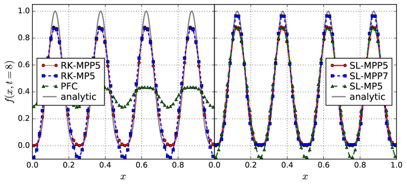
Figure 4: Test-1c (quartic sine function): profiles of the numerical solutions at $t=8$ computed with the RK schemes (left panel) and the SL schemes (right panel). For comparison, we present the result obtained with PFC in the left panel. $N_{\rm m}$n is set to 64.

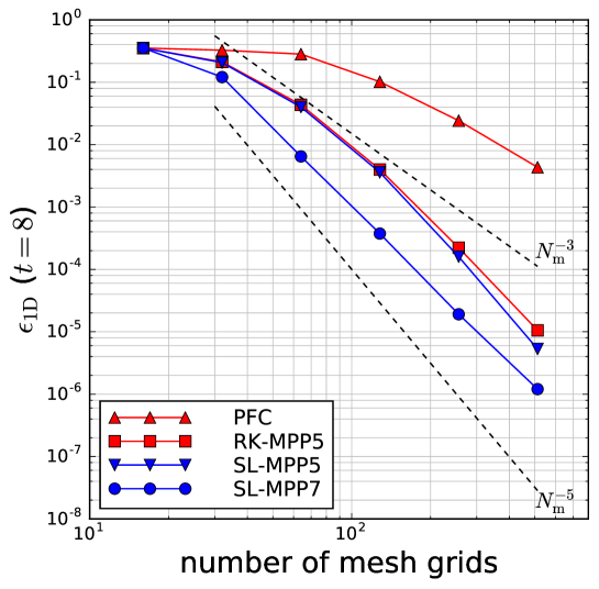
Figure 5: Test-1c (quartic sine function): relative errors of PFC, RK–MPP5, SL–MPP5, and SL–MP7. Thin dashed lines show the error scaling of third- and fifth-order accuracies from top to bottom.

3.1.4 Test-1d: Two-dimensional Advection

Here, we present numerical simulations of two-dimensional advection problems with our new schemes to test their numerical accuracy in multi-dimensional problems. We solve a two-dimensional advection equation

$$\frac{\partial f(\textbf{{x}},t)}{\partial t}+c_{x}\frac{\partial f(\textbf{{x}},t)}{\partial x}+c_{y}\frac{\partial f(\textbf{{x}},t)}{\partial y}=0,$$ (64)

where $c_{x}$ and $c_{y}$ are advection speed along the $x$- and $y$-direction, respectively. We set up a two-dimensional domain with $0\leq x,y\leq 1$ with a periodic boundary condition and consider three initial conditions similar to those presented in the one-dimensional tests: a rectangular-shaped wave given by

$$f(x,y,t=0)=\left\{\begin{array}[]{cc}1&0.25\leq x,y\leq 0.75\\ 0&{\rm otherwise}\end{array}\right.,$$ (65)

a sinusoidal wave

$$f(x,y,t=0)=1+\frac{1}{2}\sin(2\pi x)+\frac{1}{2}\sin(2\pi y)$$ (66)

and a quartic sine wave

$$f(x,y,t=0)=\sin^{4}(4\pi x)+\sin^{4}(4\pi y).$$ (67)

In all three runs, we set the advection velocities to $(c_{x},c_{y})=(1,0.5)$. The simulation domain is discretized into the Cartesian mesh grids with $N_{\rm x}$ and $N_{\rm y}$ mesh grids along the $x$- and $y$-direction, respectively.

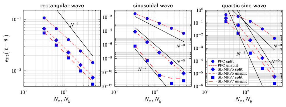
Figure 6: Test-1d (two-dimensional advection): relative errors are obtained with PFC, SL–MPP5, and SL–MPP7 in the two-dimensional advection problems. Points and dashed lines show the results obtained with the directional splitting and the unsplit methods, respectively. Solid lines indicate the scaling of relative errors with respect to the number of mesh grids as depicted in each panel.

We compute the relative error of numerical solutions to the analytic solution defined by

$$\epsilon_{\rm 2D}=\frac{\displaystyle\sum_{i=1}^{N_{\rm x}}\sum_{j=1}^{N_{\rm y}}\left|f_{i,j}-f(x_{i},y_{j},t)\right|}{\displaystyle\sum_{i=1}^{N_{\rm x}}\sum_{j=1}^{N_{\rm y}}\left|f(x_{i},y_{j},t)\right|},$$ (68)

where $f_{i,j}$ is a numerical solution at $(x,y)=(x_{i},y_{j})$ and $x_{i}$ and $y_{j}$ are the $x$ and $y$ coordinates of the $i$ and $j$th mesh grids in the $x$- and $y$-direction, respectively. Figure 6 shows the relative errors of numerical solutions obtained with PFC, SL–MPP5, and SL–MPP7 combined with the directional splitting or the unsplit methods, in which the numbers of mesh grids along each dimension are set to $N_{\rm x}=N_{\rm y}=32$, 64, 128, 256, and 512.

For the advection of a rectangular-shaped function, the scaling of the relative errors is nearly first order in space irrespective of adopted numerical schemes, while the results obtained with SL–MPP7 and SL–MPP5 are less diffusive than those obtained with PFC. On the other hand, numerical solutions of the advection of a two-dimensional sinusoidal wave obtained with PFC, SL–MPP5, and SL–MPP7 give the third-, fifth-, and seventh-order scalings of the relative error, respectively, in which the sinusoidal shape is so smooth that the MP constraint and PP limiter do not affect the overall accuracy of the schemes. In the case of a quartic sine function, the PP limiter compromises the numerical accuracy around the minima of the wave, and the numerical solutions with SL–MPP5 and SL–MPP7 exhibit nearly fifth-order accuracy, while the scaling of the relative errors obtained with the PFC scheme is not better than the third order. All these results are consistent with what we have in the one-dimensional Test-1a, Test-1b, and Test-1c, indicating that our new schemes also exhibit spatially high-order accuracies in the multidimensional problems.

As described in section 2.4, we do not adopt the unsplit method for the time integration, due to its several disadvantages against the directional splitting method. It is, however, useful to make a comparison of numerical accuracy obtained with these two methods. The relative errors obtained with the unsplit method combined with PFC, SL–MPP5, and SL–MPP7 are also shown in each panel of Figure 6. We heuristically find that the CFL parameter must be less than 0.1 in the runs with the unsplit method to keep the monotonicity and positivity of the numerical solutions, and we set $\nu=0.02$ in computing the results with the unsplit method. It is clearly seen that the unsplit method yields almost the same level of numerical errors as the directional splitting method. We also find that the computational cost in computing with the unsplit method is larger than that of the directional splitting method by $\simeq 30$% in terms of wall-clock time per step.

3.2 Test-2: Vlasov–Poisson Simulation of One-dimensional Gravitational Instability and Collisionless Damping

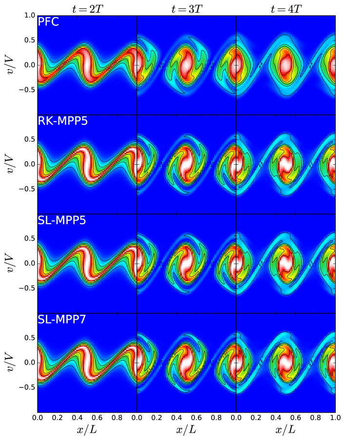
Figure 7: Test-2 (one-dimensional gravitational instability): Maps of the phase space density computed with PFC, RK–MPP5, SL–MPP5 and SL–MPP7 from top to bottom at $t=2T$, $3T$ and $4T$. We set $N_{\rm x}=N_{\rm v}=64$.

Next, we perform Vlasov–Poisson simulations of spatially one-dimensional self-gravitating systems in two-dimensional phase space volume. We consider the periodic simulation domain with $0\leq x\leq L$ and set the initial condition to be

$$f(x,v,t=0)=\frac{\bar{\rho}[1+A\cos(kx)]}{(2\pi\sigma^{2})^{1/2}}\exp\left(-\frac{v^{2}}{2\sigma^{2}}\right),$$ (69)

where $\sigma$ is the velocity dispersion, $\bar{\rho}$ is the mean density of the system, and $A$ is the amplitude of density inhomogeneity. This distribution function yields the initial mass density as

$$\rho(x)=\bar{\rho}[1+A\cos(kx)],$$ (70)

and the density inhomogeneity develops through the gravitational instability when the wavenumber $k$ satisfies the condition $k/k_{\rm J}<1$, where $k_{\rm J}$ is the Jeans wavenumber defined by

$$k_{\rm J}=\left(\frac{4\pi G\bar{\rho}}{\sigma^{2}}\right)^{1/2}.$$ (71)

In this test, we set the wavenumber $k$ to $k=4\pi/L$ and the velocity dispersion $\sigma$ so as to be $k/k_{\rm J}=0.5$, and the amplitude to $A=0.01$. The velocity space is defined over $-V\leq v\leq V$, where $V=L/T$ and $T$ is the dynamical timescale defined by $T=(G\bar{\rho})^{-1/2}$. We adopt outflow boundary conditions in the velocity space. Figure 7 shows the maps of the phase space density computed with PFC, RK–MPP5, SL–MPP5, and SL–MPP7 at $t=2T$, $3T$, and $4T$. The numbers of mesh grids in physical and velocity space are set to $N_{\rm x}=N_{\rm v}=64$. The phase space density computed with PFC with third-order spatial accuracy is significantly smeared especially at later epochs compared to the results with other spatially higher-order schemes. The results with RK–MPP5 and SL–MPP5 schemes, both of which have the spatially fifth-order accuracy, appear almost identical to each other. SL–MPP7 is able to resolve finer spiral-arm structure of matter distribution in the phase space located at the turnaround position ($x\simeq 0.35$ and $x\simeq 0.65$).

Figure 8 compares the results computed with RK–MPP5, SL–MPP5, and SL–MPP7 with the PP limiter (top panels) and with RK–MP5, SL–MP5, and SL–MP7 without it (bottom panels). The regions with negative phase space density depicted by white dots in the bottom panels are not present in the results computed with the PP limiter.

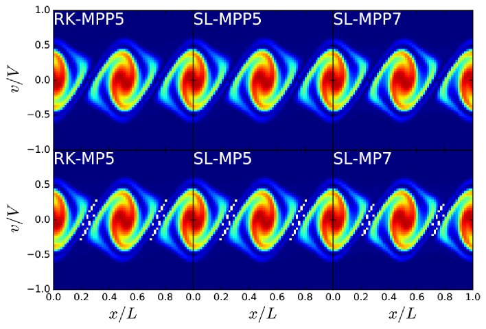
Figure 8: Test-2 (one-dimensional gravitational instability): maps of the phase space density obtained by advection schemes with and without the PP limiter. White regions in the bottom panels have negative phase space density. We set $N_{\rm x}=N_{\rm v}=64$.

To measure the accuracy of the numerical solutions obtained with various schemes, we compute the following quantity:

$$\epsilon_{\rm VP}(t)=\frac{\displaystyle\sum_{i=1}^{N_{\rm x}}\sum_{j=1}^{N_{\rm v}}|f(x_{i},v_{j},t)-f_{\rm ref}(x_{i},v_{j},t)|}{\displaystyle\sum_{i=1}^{N_{\rm x}}\sum_{j=1}^{N_{\rm v}}|f_{\rm ref}(x_{i},v_{j},t)|},$$ (72)

where $f_{\rm ref}(x,v,t)$ is a reference solution to be compared with. Since we do not have any analytical solution for this test, we construct the reference solution $f_{\rm ref}(x,v,t)$ in the following manner: First, we conduct runs with $N_{\rm x}=N_{\rm v}=4096$ using SL–MPP7 and apply the fifth-order spline interpolation to the results so that the values of the numerical distribution function can be directly compared with between different numbers of mesh grids. The left panel of Figure 9 shows the relative errors of the numerical solutions at $t=4T$ computed using PFC, RK–MPP5, SL–MPP5, and SL–MPP7 with $N_{\rm x}=N_{\rm v}=64-2048$ mesh grids. The scalings of the relative errors of our new schemes and the PFC scheme are nearly in second and first order, respectively, and somewhat compromised compared between their formal orders of accuracies, because the functional shape of the distribution function is not so smooth that the MP constraint and the PP limiter effectively work. The accuracies of RK–MPP5, SL–MPP5, and SL–MPP7 for a given number of mesh grids are significantly better than PFC with the same number of mesh grids and are similar to or even better than that with four times as many mesh grids.

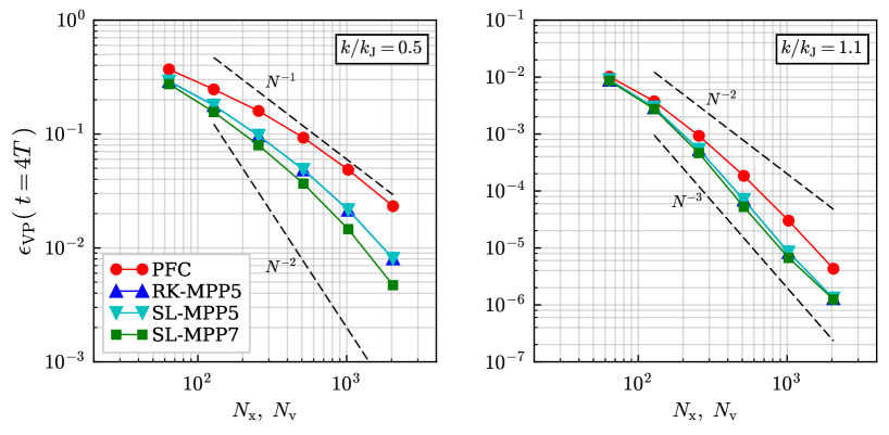
Figure 9: Test-2 (one-dimensional gravitational instability): relative errors of numerical solutions computed with the PFC, RK–MPP5, SL–MPP5, and SL–MPP7 schemes with respect to the reference solution as a function of number of mesh grids. Results with $k/k_{\rm J}=0.5$ and $1.1$ are shown in the left and right panels, respectively.

We also measure the accuracies of our new schemes in the runs with $k/k_{\rm J}=1.1$, in which the density fluctuation damps through the collisionless damping or the free streaming. In the case with $k/k_{\rm J}=1.1$, we set the amplitude of density fluctuation to $A=0.1$ and extend the velocity space as $-2V\leq v\leq 2V$ since the velocity dispersion is larger than the case with $k/k_{\rm J}=0.5$. We compute the relative errors of the distribution function at $t=4T$ in the same manner as done in the case with $k/k_{\rm J}=0.5$. The right panel of Figure 9 shows the relative errors of numerical solutions computed with our new schemes as well as PFC for $N_{\rm x}=N_{\rm v}=64-2048$ mesh grids. In this test, the shape of the distribution function is relatively smoother than the runs with $k/k_{\rm J}=0.5$, and the numerical solutions are not as strongly affected by the MP constraint and the PP limiter as the runs with $k/k_{\rm J}=0.5$. Accordingly, the scalings of the relative errors are better than those in the case with $k/k_{\rm J}=0.5$ and are nearly third and second order for our new schemes and PFC, respectively. Note that the accuracies of RK–MPP5 and SL–MPP5 are almost the same as each other in both cases with $k/k_{\rm J}=0.5$ and 1.1, indicating that the RK schemes and SL schemes yield almost the same accuracy in these tests.

3.3 Test-3: Landau Damping in Electrostatic Plasma

We perform simulations of Landau damping in an electrostatic plasma, in which the time evolution of the distribution function of electrons is described by the following Vlasov equation:

$$\frac{\partial f}{\partial t}+v\cdot\frac{\partial f}{\partial x}-\frac{e}{m}\frac{\partial\phi_{\rm s}}{\partial x}\cdot\frac{\partial f}{\partial v}=0,$$ (73)

where $\phi_{\rm s}$ is the electrostatic potential and $e$ and $m$ are the charge and mass of an electron, respectively. The electrostatic potential satisfies the Poisson equation

$$\nabla^{2}\phi_{\rm s}=4\pi ne\left(1-\int_{-\infty}^{\infty}fdv\right),$$ (74)

where $n$ is the number density of ions. In this formulation, the distribution function is normalized such that its integration over the velocity space gives the fraction of electron number density relative to ions.

We consider a two-dimensional phase space with $-2\pi L\leq x\leq 2\pi L$ and $-6V\leq v\leq 6V$, where $V\equiv\omega_{\rm pe}L$ and $\omega_{\rm pe}=(4\pi e^{2}n/m)^{1/2}$ is the electron plasma frequency and the periodic boundary condition is imposed on the physical space. The initial condition is given by

$$f(x,v,t=0)=\frac{1}{\sqrt{2\pi\sigma^{2}}}\exp\left(-\frac{v^{2}}{2\sigma^{2}}\right)(1+A\cos kx),$$ (75)

where the wavenumber is set to $k=1/(2L)$ and $\sigma=V$. With this initial condition, it is expected that the electric field damps exponentially as $\exp(-\gamma\omega_{\rm pe}t)$ with $\gamma=0.153$.

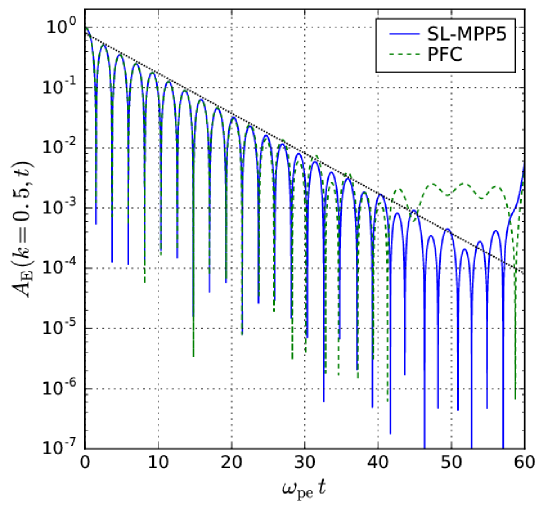
Figure 10: Test-3 (Landau damping in electrostatic plasma): time evolution of the amplitude of the electric field normalized at $t=0$. The dotted line indicates the theoretical prediction with a damping rate of $\gamma=0.153$. We set $N_{\rm x}=N_{\rm v}=64$.

First, we show results of linear Landau damping in which we set the amplitude of the initial perturbation to $A=0.01$. We set $N_{\rm x}=N_{\rm v}=64$. Figure 10 shows time evolution of the amplitude of the electric field with a mode of $k=1/(2L)$ obtained with PFC and SL–MPP5. The results obtained with RK–MPP5 and SL–MPP7 are almost identical to that of SL–MPP5 and are not presented in this figure. Although the numerical solution with PFC ceases to damp at $t\gtrsim 40\omega_{\rm pe}^{-1}$, the one obtained with the SL–MPP5 scheme continues to damp to $t\lesssim 55\omega_{\rm pe}^{-1}$, just before the recurrence time $t_{\rm R}=2\pi/(k\Delta v)=67\omega_{\rm pe}^{-1}$, indicating that SL–MPP5 is less dissipative than PFC.

Next, we perform simulations of nonlinear Landau damping with $A=0.5$. This problem has been investigated in a number of previous studies (e.g., Klimas, 1987; Manfredi, 1997; Nakamura & Yabe, 1999). In this problem, the initial perturbations damp (in space) quickly, but a highly stratified distribution in the phase space develops with time through rapid phase mixing (see Figure 11). The amplitude of the electric field initially decreases, but particle trapping by the electric field prevents complete damping. Figure 11 shows the phase space density of electrons at $t=10\,\omega_{\rm pe}^{-1}$, $20\,\omega_{\rm pe}^{-1}$, $40\,\omega_{\rm pe}^{-1}$, and $50\,\omega_{\rm pe}^{-1}$ computed with PFC, RK–MPP5, SL–MPP5, and SL–MPP7. All the results are obtained with $N_{\rm x}=64$ and $N_{\rm v}=256$. Rapid phase space mixing generates a number of peaks along the velocity axis. The PFC solution exhibits a smeared distribution at $t\gtrsim 40\,\omega_{\rm pe}^{-1}$, while those computed with other higher-order schemes preserve features of phase mixing even at $t=50\,\omega_{\rm pe}^{-1}$. This is also seen in Figure 12 in which we show the velocity distribution function

$$F(v,t)=\int f(x,v,t)dx$$ (76)

at $t=50\,\omega_{\rm pe}^{-1}$. There are a number of peaks in the velocity distribution function, which represent electrons trapped by electrostatic waves around their phase velocities. The peaks in the distribution function are more prominent in the results with fifth- and seventh-order schemes than in PFC, again showing the less dissipative nature of our schemes.

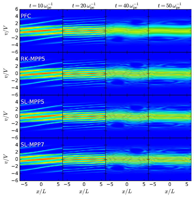
Figure 11: Test-3 (Landau damping in electrostatic plasma): maps of the phase space density of electrons in nonlinear Landau damping computed with PFC, RK–MPP5, SL–MPP5, and SL–MPP7 schemes (from top to bottom) at $t=10\omega_{\rm pe}^{-1}$, $20\omega_{\rm pe}^{-1}$, $40\omega_{\rm pe}^{-1}$ and $50\omega_{\rm pe}^{-1}$ (from left to right). Numbers of mesh grids in physical and velocity spaces are set to $N_{\rm x}=64$ and $N_{\rm v}=256$, respectively.

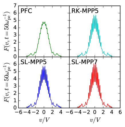
Figure 12: Test-3 (Landau damping in electrostatic plasma): velocity distribution functions in nonlinear Landau damping at $t=50\omega_{\rm pe}^{-1}$ computed with PFC, RK–MPP5, SL–MPP5, and SL–MPP7 schemes. The results are computed using the phase space density shown in Figure 11.

3.4 Test-4: Spherical Collapse of a Uniform-density Sphere

Finally, we study gravitational collapse of a uniform-density sphere. The mass and the initial radius of the sphere are $M$ and $2R$, respectively, and the initial distribution function is given by

$$f(\textbf{{x}},\textbf{{v}},t=0)=\frac{\rho_{0}}{(2\pi\sigma^{2})^{3/2}}\exp\left(-\frac{|\textbf{{v}}|^{2}}{2\sigma^{2}}\right),$$ (77)

where $\rho_{0}=M/(4\pi(2R)^{3}/3)$ is the initial density of the sphere and $\sigma^{2}=GM/(20R)$ is the initial velocity dispersion of the matter inside the sphere. We set the initial virial ratio to be 0.5. The extent of the simulation volume is $-3R\leq x,y,z\leq 3R$ in the physical space and $-3V\leq v_{x},v_{y},v_{z}\leq 3V$, where $V$ is given by $V=R/T$ and $T=(R^{3}/GM)^{1/2}$ is the dynamical timescale of the system. In this test, we adopt the out-going boundary condition in both the physical and velocity spaces. We perform the runs with $N_{\rm x}=64^{3}$ for the physical space and $N_{\rm v}=32^{3}$ or $N_{\rm v}=64^{3}$ mesh grids for the velocity space.

We plot the phase space density in the $(x,v_{x})$-plane with $y=z=0$ and $v_{y}=v_{z}=0$ at $t=3T$, $4T$, $6T$ and $8T$ in Figure 13. We set $N_{\rm x}=N_{\rm v}=64^{3}$. Initially, the sphere starts to collapse toward the center and reaches the maximum contraction around $t=4T$. Then the system expands again, and a part of the matter passes through the center of the system to reache the outer boundary of the physical space defined at $x=\pm 3R$, $y=\pm 3R$, and $z=\pm 3R$. The results computed with PFC show smeared distribution compared with those obtained with RK–MPP5, SL–MPP5, and SL–MPP7. We note that RK–MPP5 and SL–MPP5 yield almost identical results, although the computational costs for the two are significantly different (see § 4).

Figure 14 is the same plot as Figure 13 but shows the results with $N_{\rm v}=32^{3}$. It is interesting that the results obtained by SL–MPP7 with $N_{\rm x}=64^{3}$ and $N_{\rm v}=32^{3}$ (bottom panels in Figure 14) are similar to or even better than those obtained with PFC with $N_{\rm x}=N_{\rm v}=64^{3}$ (top panels in Figure 13), despite the eight times smaller number of mesh grids.

For this test, we compare our new schemes with another independent scheme. To this end, we utilize a high-resolution $N$-body simulation in the following manner. First, we perform an $N$-body simulation starting from the initial condition equivalent to Equation (77). In this $N$-body simulation, the gravitational potential field is dumped and stored at all the time steps. Then, we compute the phase space density at a given phase space coordinate $(\textbf{{x}}(t),\textbf{{v}}(t))$ by tracing back the coordinate to its initial coordinate $(\textbf{{x}}(0),\textbf{{v}}(0))$ using the previously stored gravitational potentials. Since the phase space density is constant along each trajectory, we can, in principle, compute the phase space density from the initial phase space coordinate $(\textbf{{x}}(0),\textbf{{v}}(0))$ using Equation (77). However, trajectories in conventional $N$-body simulations are subject to rather grainy gravitational potential compared to what it should be in the actual physical system owing to their superparticle approximation. Thus, we adopt the self-consistent field (SCF) method (Hernquist & Ostriker, 1992; Hozumi, 1997), in which the gravitational potential is computed by expanding the density field into a set of basis functions, and particle trajectories are calculated for the smooth gravitational potential. The initial condition is constructed with $10^{7}$ equal-mass particles, and the particle orbits are computed using the basis set constructed by Clutton-Brock (1972), where the numbers of the expansion terms are 64 and 144 in the radial and angular directions, respectively. Figure 15 shows the phase space density obtained with this procedure. Comparing with Figures 13 and 14 manifests that our spatially higher-order schemes (RK–MPP5, SL–MPP5, and SL–MPP7) yield results much closer to those obtained with the SCF approach. It should be noted that, in practice, the SCF method is applicable only to self-gravitating systems with a certain spatial symmetry, such as in the present test, to which the lowest-order functions of the basis set suffice to describe the overall structure of the system. Also, storing the gravitational potential (or its expansion) at all the time steps is very costly. Therefore, the SCF approach cannot be applied to a wide range of self-gravitating systems. For further comparison with the results obtained by the SCF methods, we perform a Vlasov–Poisson run with the largest numbers of mesh grids, $N_{\rm x}=128^{3}$ and $N_{\rm v}=128^{3}$ using SL–MPP5, and show the phase space density at $t=3T$, $4T$, $6T$ and $8T$ in the $(x,v_{x})$-plane in Figure 16. With such high resolution, the phase space density is consistent with that obtained with the SCF method in detail.

Figure 13: Test-4 (spherical collapse of a uniform-density sphere): phase space density in the ($x$,$v_{x}$)-plane with $y=z=0$ and $v_{y}=v_{z}=0$ computed with PFC, RK–MPP5, SL–MPP5, and SL–MPP7 at $t=3T$, $4T$, $6T$, and $8T$. The number of mesh grids is $64^{3}$ in the physical space and $64^{3}$ in the velocity space.

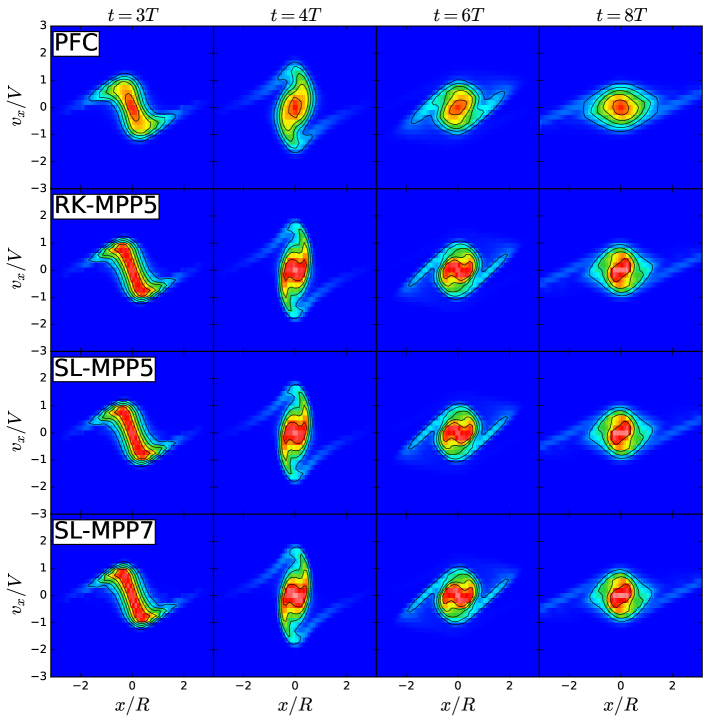
Figure 14: Test-4 (spherical collapse of a uniform-density sphere): same as Figure 13 except that the number of mesh grids in the velocity space is $32^{3}$.

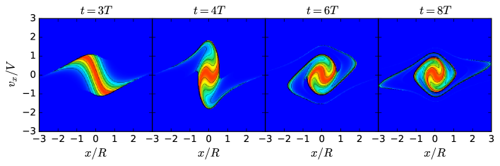
Figure 15: Test-4 (spherical collapse of a uniform-density sphere): same as Figure 13 except that the self-consistent field method is used instead of the Vlasov–Poisson simulation.

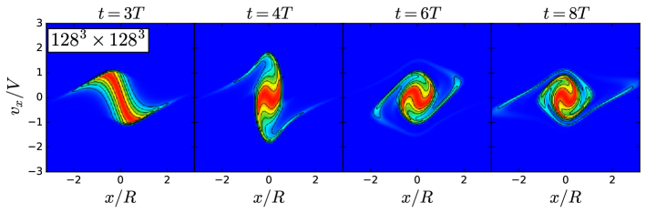
Figure 16: Test-4 (spherical collapse of a uniform density sphere): same as Figure 13 except that the number of mesh grids is $N_{\rm x}=128^{3}$ and $N_{\rm v}=128^{3}$. The SL–MPP5 scheme is used for the simulation.

We further examine the mass and energy conservation for this spherical collapse test. We show the time evolution of the total mass, kinetic energy, and gravitational potential energy of the results simulated with PFC and SL–MPP5 in Figure 17, where the results obtained with $N_{\rm v}=64^{3}$ and $N_{\rm v}=32^{3}$ are shown in the left and right panels, respectively. Note that the results simulated with RK–MPP5 and SL–MPP7 are almost the same as those of SL–MPP5 and hence are not shown in this figure. For comparison, we also plot the results obtained with an $N$-body simulation, in which we employ $128^{3}$ particles, and adopt the Particle-Mesh (PM) method with the number of mesh grids in solving the Poisson equation equal to that of the Vlasov–Poisson simulation, i.e., 64 mesh grids in each dimension, in order to realize the same spatial resolution of the gravitational field and force. The total mass in the Vlasov simulation starts to decrease around $t\simeq 8T$ because a part of the matter reaches the boundary of the simulation volume at that time, as can be seen in Figures 15 and  16. In the runs with PFC, such a decrease of the total mass begins earlier and the amount of the escaped mass is larger than that in the runs with SL–MPP5 and other higher-order schemes owing to larger numerical diffusion, irrespective of $N_{\rm v}$. The most prominent difference can be seen around the maximum contraction epoch $t\simeq 4T$, when the kinetic and gravitational potential energies have their maximum and minimum values, respectively. As can be seen in Figures 13 and 14, the large numerical diffusion of PFC, in both the physical and velocity spaces, smears the “S”-shaped phase space distribution and enlarges the physical extent of the system at $t=4T$, yielding small kinetic and shallow gravitational potential energies seen in Figure 17. The overall accuracy can be improved for PFC by simply increasing the number of mesh grids from $N_{\rm v}=32^{3}$ to $64^{3}$. On the other hand, the result of SL–MPP5 is close to the $N$-body simulation, irrespective of $N_{\rm v}$, and in the runs with $N_{\rm v}=64^{3}$ both of the results with PFC and SL–MPP5 are in good agreement with the $N$-body simulation. This suggests that SL–MPP5 (as well as RK–MPP5 and SL–MPP7) with $N_{\rm v}=32^{3}$ provides roughly the same level of accuracy as PFC with $N_{\rm v}=64^{3}$ in terms of mechanical energy.

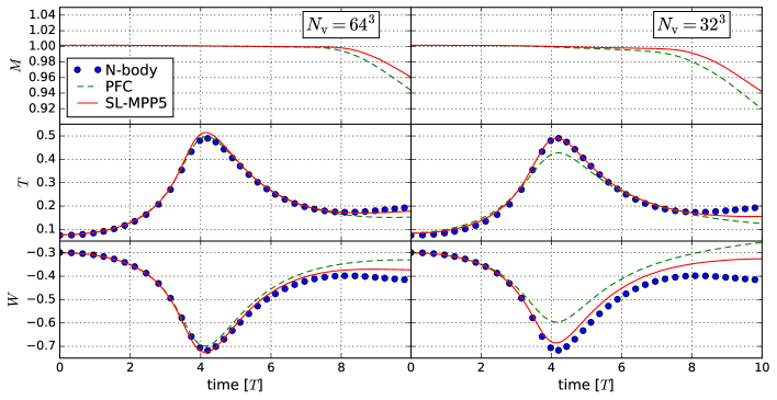
Figure 17: Test-4 (spherical collapse of a uniform-density sphere): time evolution of the total mass (top), kinetic energy (middle), and potential energy (bottom) in the runs with $N_{\rm v}=64^{3}$ (left) and $N_{\rm v}=32^{3}$ (right) computed with PFC and SL–MPP5. The kinetic and gravitational potential energies obtained with an $N$-body simulation are also shown for the comparison.

4 Computational Cost

In addition to the computational accuracy, we need to address the computational speed of our new schemes. We measure the wall-clock time to advance each of Equation (4) and (5) by a single time step using PFC, RK–MPP5, SL–MPP5, and SL–MPP7 for various combinations of $N_{\rm x}$ and $N_{\rm v}$ ranging from $32^{3}$ to $128^{3}$ on 64 nodes of the HA-PACS system at Center for Computational Sciences, University of Tsukuba. The largest number of mesh grids adopted in this measurement is $(N_{\rm x},N_{\rm v})=(128^{3},64^{3})$. Figure 18 shows the measured wall-clock time per mesh grid in six-dimensional Vlasov–Poisson simulations of the growth of gravitational instability from a nearly uniform-density distribution that is identical to Test-4 in YYU13. We show the wall-clock time to advance the advection equations in the physical space (Equation (4)) and those in the velocity space (Equation (5)) in the left and right panels, respectively. One can see that RK–MPP5 is the most computationally expensive among all the advection schemes described in this work. This is largely because it performs three-stage RK time integration (Equation (10)) and computes numerical fluxes three times per step while other schemes need only single-stage time integration (Equation (49)). Since the physical space is divided into subdomains and stored in independent memory spaces, solving advection Equation (4) in the physical space requires internode communications to transfer phase space densities to/from adjacent computational nodes and thus takes a longer wall-clock time than solving Equation (5) in the velocity space. The computational costs of SL–MPP5 and SL–MPP7 are significantly smaller than that of RK–MPP5 and are almost the same as that of PFC.

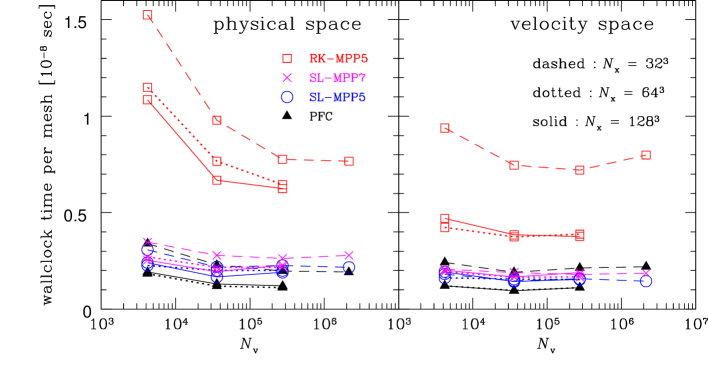
Figure 18: Wall-clock times per mesh grid for a single step of advection in the physical space (left panel) and the velocity space (right panel) computed with PFC (filled triangles), RK–MPP5 (open squares), SL–MPP5 (open circles), and SL–MPP7 (crosses). Data connected with solid, dotted, and dashed lines are measured in runs with $N_{\rm x}=32^{3}$, $64^{3}$ and $128^{3}$, respectively.

5 Summary and Conclusion

In this work, we present a set of new spatially fifth- and seventh-order advection schemes developed for Vlasov simulations that preserve both of monotonicity and positivity of numerical solutions. The schemes are based on the spatially fifth-order MP scheme proposed by Suresh & Huynh (1997) combined with the three-stage TVD–RK scheme and are extended so that they also preserve positivity by using a flux limiter. We also devise an alternative approach to construct MP and PP schemes by adopting the SL time integration scheme, for the substitution of the three-stage TVD–RK scheme. With this approach, we are able to adopt spatially seventh- or higher-order schemes without using computationally expensive fourth- or higher-order TVD–RK time integration schemes and hence to reduce the computational cost.

We perform an extensive set of numerical tests to verify the improvement of numerical solutions using our newly developed schemes. The test suite includes one- and two-dimensional linear advection problems, one-dimensional collisionless self-gravitating and electrostatic plasma systems in two-dimensional phase space, and a three-dimensional self-gravitating system in six-dimensional phase space. The results are compared with those obtained with the spatially third-order PFC scheme adopted in our previous work (Yoshikawa et al., 2013) and are summarized as follows.

In Test-1, we present calculations of one-dimensional linear advection problems and confirm that numerical solutions computed with our new schemes have better accuracy than PFC. The PP limiter works well in every advection test, although it introduces a slight degradation of numerical accuracy in terms of the error scaling in combination with the TVD Runge-Kutta time integration scheme. It is found that the SL time integration provides us with better numerical accuracy than the TVD–RK scheme and that the combination of the PP limiter and the SL time integration does not introduce any expense of numerical accuracy unlike the TVD–RK time integration. It should be noted that the spatially seventh-order RK–MPP7 exhibits undesirable features in the advection of a rectangular-shaped function originating from insufficient accuracy of the three-stage RK time integration scheme, and that the numerical solutions obtained with SL–MPP7 contrastingly do not have such features, indicating that the SL approach is crucial for constructing schemes with spatially seventh- or higher-order accuracy. Numerical solutions of two-dimensional linear advection problems computed with our new semi-Lagrangian schemes are consistent with those in the one-dimensional ones, proving that our new schemes work well also in multidimensional problems.

In Test-2 and Test-3, we perform Vlasov–Poisson simulations of a one-dimensional self-gravitating and electrostatic plasma systems in two-dimensional phase space, respectively. In the self-gravitating system, we found that the phase space density distribution simulated with the PFC scheme is significantly suffered from numerical diffusion compared with those simulated with our new schemes. In terms of the $L^{1}$ error of the distribution function, the fifth-order schemes (RK–MPP5 and SL–MPP5) yield almost identical results and achieve almost the same level of numerical accuracy as the third-order scheme with four times refined mesh grids, while the spatially seventh-order SL–MPP7 is proved to be the most accurate scheme among all the schemes presented in this work. In addition, the PP limiter also works well in the Vlasov simulations. In the simulations of electrostatic plasma, we perform the linear and nonlinear Landau damping problems. In the former, we found that numerical solution computed with the third-order scheme ceases damping sufficiently before the recurrence time, due to its large numerical diffusion. On the other hand, the numerical solutions with our new schemes continue to damp just before the recurrence time. As for the nonlinear Landau damping, the highly stratified distribution formed through rapid phase mixing is well solved with our new schemes, while it is strongly smeared in the numerical solution computed with PFC, due to its large numerical diffusion.

Finally, in Test-4 we perform Vlasov–Poisson simulations of a fully three-dimensional self-gravitating system in a six-dimensional phase space, in which runs with two different sets of numerical resolution $(N_{\rm x},N_{\rm v})=(64^{3},64^{3})$ and $(N_{\rm x},N_{\rm v})=(64^{3},32^{3})$ are conducted. By comparing the distribution functions obtained with the Vlasov–Poisson simulation with the reference solution obtained by exploiting the SCF method, one can see that our new schemes yield better numerical solutions than the third-order scheme, and the advantages of these schemes are confirmed also in Vlasov simulations in six-dimensional phase space. Comparison of the results between the runs with two different numerical resolutions tell us that our new schemes yield numerical solutions equivalent to those obtained by the third-order PFC scheme with eight times refined mesh grids. We also perform a Vlasov–Poisson simulation with $128^{3}$ mesh grids each for the spatial and velocity space, $128^{6}$ mesh grids in total, which successfully produce the apparently same phase space distribution as that obtained by exploiting the SCF method.

As for the computational costs of our new schemes, RK–MPP5 is the most expensive and requires two to three times longer wall-clock time to advance a single time step than other schemes. This is mainly because it adopts the three-stage TVD–RK time integration scheme and operates the Eulerian time integration three times per step. On the other hand, the SL schemes perform only a single Eulerian time integration per step; hence, their computational costs are significantly less expensive than RK–MPP5 and are nearly the same as that of PFC, indicating that the SL schemes achieve the improvement of effective spatial resolution without a significant increase of computational costs.

Among all the new schemes described in this paper, the spatially seventh-order SL scheme (SL–MPP7) is the most favored one in terms of numerical accuracy and computational cost, although the spatially fifth-order SL scheme can be a viable option when the capacity of internode communication is not sufficient. As a similar scheme to SL schemes, Qiu & Christlieb (2010) and Qiu & Shu (2011) develop conservative semi-Lagrangian WENO schemes to solve the Vlasov equation that adopt weighted essentially non-oscillatory (WENO) reconstruction to compute the interface values instead of the MP reconstruction adopted in our schemes. The WENO reconstruction is, however, known to be more diffusive and more computationally expensive compared with the MP scheme (Suresh & Huynh, 1997).

Since Vlasov simulations require a huge amount of memory to store the distribution function in six-dimensional phase space volume, the size of Vlasov simulations is mainly limited by the amount of total available memory rather than the computational cost. Adoption of spatially higher-order advection schemes in Vlasov simulations enables us to effectively improve the numerical resolution without increasing the number of mesh grids. In this sense, our new spatially higher-order advection schemes are of crucial importance in numerically solving Vlasov equations. We implement our new advection schemes to Vlasov–Poisson simulations that can be applied to collisionless self-gravitating and electrostatic plasma systems and we confirmed that our schemes really improve the numerical accuracies of Vlasov–Poisson simulations for a given number of mesh grids. Though we have applied our schemes only to Vlasov–Poisson simulations, we are going to apply our schemes to Vlasov–Maxwell simulations for magnetized plasma systems in a future work, in which difficulties in following gyro motion around magnetic field lines or an advection by rigid rotation in velocity space have been reported by many authors (Minoshima et al., 2011, 2013, 2015).

We thank Professor Shunsuke Hozumi for providing distribution function data of Test-4 computed with his SCF code and for his valuable comments on this work. This research is supported by MEXT as “Priority Issue on Post-K computer” (Elucidation of the Fundamental Laws and Evolution of the Universe) and JICFuS and uses computational resources of the K computer provided by the RIKEN Advanced Institute for Computational Science through the HPCI System Research project (project ID:hp160212 and hp170231). This research used computational resources of the HPCI system provided by Oakforest–PACS through the HPCI System Research Project (project ID:hp170123). Part of the numerical simulations are performed using HA-PACS and COMA systems at Center for Computational Sciences, University of Tsukuba, and Cray XC30 at Center for Computational Astrophysics, National Astronomical Observatory of Japan.

Appendix A Monotonicity-preserving Constraint

The MP scheme devised by Suresh & Huynh (1997) computes the interface value $f_{i+1/2}^{\rm MP}$ at a mesh boundary between the $i$th and $(i+1)$th mesh grids with five stencil values, three in the upwind side, and two in the downwind side in the following procedures:

1. Evaluate the interpolated interface value $f_{i+1/2}^{\rm int}$ at a mesh interface using an equation. In the case of MP5 or MP7 schemes, for example, we adopt Equation (9) or Equation (24) in the fifth- or seventh-order accuracy, respectively.

2. Evaluate $f^{\rm*}=f_{i}+{\rm minmod}(f_{i+1}-f_{i},\alpha(f_{i}-f_{i-1}))$, where a parameter $\alpha$ controls the upper bound of the interface value and should hold the condition $\alpha\geq 2$. Throughout in this work, we set $\alpha=4$, unless otherwise stated.

3. If the condition $(f_{i+1/2}^{\rm int}-f_{i})(f_{i+1/2}^{\rm int}-f^{\rm*})<0$ holds, the resultant interface value is given by $f_{i+1/2}^{\rm MP}=f^{\rm int}_{i+1/2}$. If not, we should proceed to the next step.

4. Compute $d_{i+1/2}^{\rm M4}\equiv{\rm minmod}(4d_{i}-d_{i+1},4d_{i+1}-d_{i},d_{i},d_{i+1})$ and $d_{i-1/2}^{\rm M4}$, where $d_{i}=f_{i-1}+f_{i+1}-2f_{i}$.

5. Compute $f^{\rm UL}\equiv f_{i}+\alpha(f_{i}-f_{i-1})$, $f^{\rm AV}\equiv(f_{i}+f_{i+1})/2$, $f^{\rm MD}\equiv f^{\rm AV}-d^{\rm M4}_{i+1/2}/2$ and $f^{\rm LC}\equiv f_{i}+(f_{i}-f_{i-1})/2+4d_{i-1/2}^{\rm M4}/3$

6. Compute $f^{\rm min}\equiv\max(\min(f_{i},f_{i+1},f^{\rm MD}),\min(f_{i},f^{\rm UL},f^{\rm LC}))$ and $f^{\rm max}\equiv\min(\max(f_{i},f_{i+1},f^{\rm MD}),\max(f_{i},f^{\rm UL},f^{\rm LC}))$.

7. Finally, the interface value is given by $f^{\rm MP}_{i+1/2}={\rm median}(f^{\rm int}_{i+1/2},f^{\rm min},f^{\rm max})$.

It should be noted that the time step constraint to keep the monotonicity of numerical solutions depends on the parameter $\alpha$ and that the CFL parameter should satisfy the condition (Suresh & Huynh, 1997)

$$\nu\leq 1/(1+\alpha)=1/5,$$ (A1)

if we set the parameter $\alpha$ to $\alpha=4$ as recommended in Suresh & Huynh (1997), although $\nu=0.4$ works well in practice. (see Appendix B for further argument on a viable range of the CFL parameter).

Appendix B CFL Condition

As noted in Appendix A, the choice of $\alpha$ and $\nu$ is rather heuristic in the MP scheme. Therefore, we also optimize the combination of $\alpha$ and $\nu$ in our new schemes RK–MPP5, SL–MPP5, and SL–MPP7 with the PP limiter in a heuristic manner. We perform Test-1c (linear advection of $\sin^{4}(4\pi x)$) using RK–MPP5, SL–MPP5, and SL–MPP7 with various combinations of $\alpha$ and $\nu$. The number of mesh grids is set to 128. Figure 19 shows maps of relative $L^{1}$ errors of Test-1c obtained with the three schemes for $0<\alpha<5$ and $0<\nu<1$. Comparison of RK–MPP5 and SL–MPP5 shows that SL–MPP5 allows us to adopt a larger CFL parameter $\nu$ than RK–MPP5 to achieve a certain accuracy. Furthermore, errors obtained with SL–MPP5 are almost unchanged irrespective of the adopted CFL parameter as long as $2<\alpha$ and $\nu<0.4$, probably in virtue of its semi-Lagrangian nature. The SL–MPP7 scheme exhibits more accurate results than the SL–MPP5 scheme for $2<\alpha$ and $\nu<0.4$, and the parameter space that yields the most accurate results is located in the vicinity of the relation $\nu=1/(1+\alpha)$.

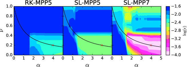
Figure 19: Maps of relative $L^{1}$ errors of Test-1c obtained with the RK–MPP5 (left), SL–MPP5 (middle), and SL–MPP7 (right) schemes for ranges of $0<\alpha<5$ and $0<\nu<1$. Solid curves and red crosses indicate the relation $\nu=1/(1+\alpha)$ and $(\alpha,\nu)=(4,0.2)$, respectively.

Appendix C The High-order Poisson solver

We derive the Green function of the discretized Poisson equation in spatially second-, fourth-, and sixth-order accuracy. Here, just for the simplicity, we only consider the one-dimensional Poisson equation. The extension to the multidimensional one is quite straightforward. Given the discrete density field $\rho_{j}$ with $0\leq j\leq N_{\rm m}-1$, where $N_{\rm m}$ is the number of mesh grids, approximating the Poisson equation with the second-order discretization leads to

$$\frac{\phi_{j+1}-2\phi_{j}+\phi_{j-1}}{\Delta x^{2}}=4\pi G\rho_{j}.$$ (C1)

Discrete Fourier transformation (DFT) of Equation (C1) yields

$$\hat{\phi}_{k}[\exp(ik\Delta x)-2+\exp(-ik\Delta x)]=4\pi G\Delta x^{2}\hat{\rho}_{k}$$ (C2)

and $\hat{\phi}_{k}$ can be expressed as

$$\hat{\phi}_{k}=-\frac{\pi G\Delta x^{2}}{\displaystyle\sin^{2}\left(\frac{k\Delta x}{2}\right)}\hat{\rho}_{k},$$ (C3)

where the ‘hat’ denotes the DFT of physical quantities expressed as

$$\hat{q}_{k}=\sum_{j=0}^{N_{\rm m}-1}q_{j}\exp(-ikj\Delta x),$$ (C4)

and $k=2\pi n/(N_{\rm m}\Delta x)$ is the discrete wavenumber, and the periodic boundary condition $\phi_{j}=\phi_{N_{\rm m}+j}$ is assumed. The discrete Poisson equations in the fourth- and sixth-order accuracy are given by

$$\frac{-\phi_{j+2}+16\phi_{j+1}-30\phi_{j}+16\phi_{j-1}-\phi_{j-2}}{12\Delta x^{2}}=4\pi G\rho_{j}$$ (C5)

and

$$\frac{2\phi_{j+3}-27\phi_{j+2}+270\phi_{j+1}-490\phi_{j}+270\phi_{j-1}-27\phi_{j-2}+2\phi_{j-3}}{180\Delta x^{2}}=4\pi G\rho_{j},$$ (C6)

respectively. Therefore, the corresponding Fourier-transformed potentials can be derived as

$$\hat{\phi}_{k}=\frac{12\pi G\Delta x^{2}}{\sin^{2}(k\Delta x)-16\sin^{2}(k\Delta x/2)}\,\hat{\rho}_{k}$$ (C7)

and

$$\hat{\phi}_{k}=-\frac{180\pi G\Delta x^{2}}{\displaystyle 2\sin^{2}\left(\frac{3k\Delta x}{2}\right)-27\sin^{2}(k\Delta x)+270\sin^{2}\left(\frac{k\Delta x}{2}\right)}\,\hat{\rho}_{k},$$ (C8)

respectively.

Gravitational force is numerically obtained with the FDA of the gradient of the gravitational potential. Use of the higher-order Poisson solvers motivates us to adopt higher-order FDAs for the gravitational force. The gradient of the gravitational potential at $x=x_{i}$ is approximated as

$$\nabla\phi|_{x=x_{i}}=\frac{\phi_{i+1}-\phi_{i-1}}{2\Delta x}+O(\Delta x^{2}),$$ (C9)

$$\nabla\phi|_{x=x_{i}}=\frac{\phi_{i+2}-8\phi_{i+1}+8\phi_{i-1}-\phi_{i-2}}{12\Delta x}+O(\Delta x^{4}),$$ (C10)

and

$$\nabla\phi|_{x=x_{i}}=\frac{\phi_{i+3}-9\phi_{i+2}+45\phi_{i+1}-45\phi_{i-1}+9\phi_{i-2}-\phi_{i-3}}{60\Delta x}+O(\Delta x^{6})$$ (C11)

with the two-, four-, and six-point FDAs, respectively.

To check the numerical accuracy of the gravitational potential and force obtained with the numerical schemes described above, we solve the one-dimensional Poisson equation with the periodic boundary condition under the density field given by

$$\rho(x)=\bar{\rho}\left[1+A\sin(kx)\right],$$ (C12)

in the domain $0\leq x<L$, where the wavenumber $k$ is set to $k=32\pi/L$, and we have 16 waves in the domain. The gravitational potential and force can be analytically solved as

$$\phi(x)=-\frac{4\pi G\bar{\rho}A}{k^{2}}\sin(kx)$$ (C13)

and

$$f(x)=-\frac{\partial\phi(x)}{\partial x}=\frac{4\pi G\bar{\rho}A}{k}\cos(kx),$$ (C14)

respectively. Figure 20 shows the relative errors of gravitational potentials and forces defined by

$$\epsilon_{\rm pot}=\frac{1}{N_{\rm m}}\sum^{N_{\rm m}-1}_{j=0}|\phi_{j}-\phi(x_{j})|$$ (C15)

and

$$\epsilon_{\rm f}=\frac{1}{N_{\rm m}}\sum^{N_{\rm m}-1}_{j=0}|f_{j}-f(x_{j})|,$$ (C16)

respectively. Note that the gravitational forces are computed with an FDA scheme with the same order of accuracy as the Poisson solver, i.e., the gravitational forces with the second-order accuracy are computed with the gravitational potentials calculated with the second-order Poisson solver through the second-order FDA scheme. It can be seen that both of the gravitational potentials and forces have the expected order of the accuracy.

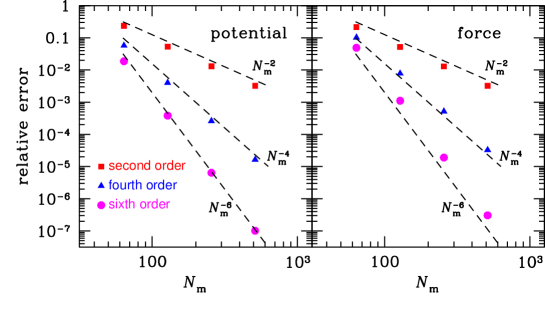
Figure 20: Relative errors of gravitational potentials (left panel) and forces (right panel) computed with spatially second-, fourth-, and sixth-order schemes for $N_{\rm m}=64,128,256$, and $512$. Dashed lines show the scalings of the second-, fourth-, and sixth-order accuracies from top to bottom.

References

- Abel et al. (2012) Abel, T., Hahn, O., & Kaehler, R. 2012, MNRAS, 427, 61
- Birdsall & Langdon (1991) Birdsall, C. K., & Langdon, A. B. 1991, Plasma Physics via Computer Simulation (New York: McGraw-Hill)
- Clutton-Brock (1972) Clutton-Brock, M. 1972, Ap&SS, 16, 101
- Filbet et al. (2001) Filbet, F., Sonnendrücker, E., & Bertrand, P. 2001, Journal of Computational Physics, 172, 166
- Fujimoto (2014) Fujimoto, K. 2014, Geophys. Res. Lett., 41, 2721
- Fujiwara (1981) Fujiwara, T. 1981, PASJ, 33, 531
- Hahn et al. (2013) Hahn, O., Abel, T., & Kaehler, R. 2013, MNRAS, 434, 1171
- Hernquist & Ostriker (1992) Hernquist, L., & Ostriker, J. P. 1992, ApJ, 386, 375
- Hockney & Eastwood (1981) Hockney, R. W., & Eastwood, J. W. 1981, Computer Simulation Using Particles (New York: McGraw-Hill)
- Hozumi (1997) Hozumi, S. 1997, ApJ, 487, 617
- Hu et al. (2013) Hu, X. Y., Adams, N. A., & Shu, C.-W. 2013, Journal of Computational Physics, 242, 169
- Janin (1971) Janin, G. 1971, A&A, 11, 188
- Kates-Harbeck et al. (2016) Kates-Harbeck, J., Totorica, S., Zrake, J., & Abel, T. 2016, Journal of Computational Physics, 304, 231
- Klimas (1987) Klimas, A. J. 1987, Journal of Computational Physics, 68, 202
- Manfredi (1997) Manfredi, G. 1997, Physical Review Letters, 79, 2815
- Matsumoto et al. (2015) Matsumoto, Y., Amano, T., Kato, T. N., & Hoshino, M. 2015, Science, 347, 974
- Minoshima et al. (2011) Minoshima, T., Matsumoto, Y., & Amano, T. 2011, Journal of Computational Physics, 230, 6800
- Minoshima et al. (2013) —. 2013, Journal of Computational Physics, 236, 81
- Minoshima et al. (2015) —. 2015, Computer Physics Communications, 187, 137
- Mitchell et al. (2013) Mitchell, N. L., Vorobyov, E. I., & Hensler, G. 2013, MNRAS, 428, 2674
- Nakamura & Yabe (1999) Nakamura, T., & Yabe, T. 1999, Computer Physics Communications, 120, 122
- Nishida et al. (1981) Nishida, M. T., Yoshizawa, M., Watanabe, Y., Inagaki, S., & Kato, S. 1981, PASJ, 33, 567
- Qiu & Christlieb (2010) Qiu, J.-M., & Christlieb, A. 2010, Journal of Computational Physics, 229, 1130
- Qiu & Shu (2011) Qiu, J.-M., & Shu, C.-W. 2011, Journal of Computational Physics, 230, 863
- Shandarin et al. (2012) Shandarin, S., Habib, S., & Heitmann, K. 2012, Phys. Rev. D, 85, 083005
- Suresh & Huynh (1997) Suresh, A., & Huynh, H. 1997, Journal of Computational Physics, 136, 83
- Vorobyov & Theis (2006) Vorobyov, E. I., & Theis, C. 2006, MNRAS, 373, 197
- Yoshikawa et al. (2013) Yoshikawa, K., Yoshida, N., & Umemura, M. 2013, ApJ, 762, 116