Exploring the climate of Proxima B with the Met Office Unified Model

We present results of simulations of the climate of the newly discovered planet Proxima Centauri B, performed using the Met Office Unified Model (UM). We examine the responses of both an ‘Earth-like’ atmosphere and simplified nitrogen and trace carbon dioxide atmosphere to the radiation likely received by Proxima Centauri B. Additionally, we explore the effects of orbital eccentricity on the planetary conditions using a range of eccentricities guided by the observational constraints. Overall, our results are in agreement with previous studies in suggesting Proxima Centauri B may well have surface temperatures conducive to the presence of liquid water. Moreover, we have expanded the parameter regime over which the planet may support liquid water to higher values of eccentricity ($\gtrsim 0.1$) and lower incident fluxes ($881.7$ W m^-2) than previous work. This increased parameter space arises because of the low sensitivity of the planet to changes in stellar flux, a consequence of the stellar spectrum and orbital configuration. However, we also find interesting differences from previous simulations, such as cooler mean surface temperatures for the tidally-locked case. Finally, we have produced high resolution planetary emission and reflectance spectra, and highlight signatures of gases vital to the evolution of complex life on Earth (oxygen, ozone and carbon dioxide).

1 Introduction

Motivated by the grander question of whether life on Earth is unique, since the detection of the first exoplanet Wolszczan & Frail (1992); Mayor & Queloz (1995), efforts have become increasingly focused on ‘habitable’ planets. In order to partly side-step our ignorance of the possibly vast range of biological solutions to life, and exploit our mature understanding of our own planet’s climate, we define the term ‘habitable’ in a very Earth-centric way. Informed by the ‘habitable zone’ first defined by Kasting (1988), we have searched for planets where liquid water, so fundamental to Earth-life, might be present on the planetary surface. The presence of liquid water is likely to depend on a large number of parameters such as initial water budget, atmospheric composition, flux received from the host star etc. Of course, the more ‘Earth-like’ the exoplanet, the more confidence we have in applying adaptations of our theories and models developed to study Earth itself, and thereby predicting parameters such as surface temperature and precipitation. Surveys such as the Terra Hunting Experiment Thompson et al. (2016) aim to discover targets similar in both mass and orbital configuration to Earth, but also orbiting stars similar to our Sun, for which follow-up characterisation measurements might be possible.

In the meantime, observational limitations have driven the search for ‘Earth-like’ planets to lower mass, and smaller radius stars i.e. M-Dwarfs (e.g. MEarth, Nutzman & Charbonneau, 2008). Such stars are much cooler and fainter than our own Sun, so potentially habitable planets must exist in much tighter orbits. Recent, ground breaking, detections have been made for potentially “Earth-like” planets in orbit around M-Dwarfs (e.g. Gliese 581g Vogt et al. (2010), Kepler 186f Quintana et al. (2014), the Trappist 1 system Gillon et al. (2016)). In fact, such a planet has been discovered orbiting, potentially in the ‘habitable zone’ of our nearest neighbour Proxima Centauri Anglada-Escude et al. (2016), called Proxima Centauri B (hereafter, ProC B).

The announcement of this discovery was coordinated with a comprehensive modelling effort, exploring the possible effects of the stellar activity on the planet over its evolution and its budget of volatile species Ribas et al. (2016), and a full global circulation model (GCM) of the climate Turbet et al. (2016). Of course, lessons from solar system planets Forget & Lebonnois (2013) and our own Earth-climate Flato et al. (2013) have taught us that the complexity of GCMs can lead to model dependency in the results. This can often be due to subtle differences in the numerics, various schemes (i.e. radiative transfer, chemistry, clouds etc.) or boundary and initial conditions. Goldblatt (2016) provides an excellent resource, using 1D models and limiting concepts with which to aid conceptual understanding of the habitability of ProC B, highly complementary to results from more complex 3D models such as Turbet et al. (2016) and this work.

In this work we apply a GCM of commensurate pedigree and sophistication to that used by Turbet et al. (2016) to ProC B and explore differences due to the model, and extend the exploration to a wider observationally plausible parameter space. The GCM used is the Met Office Unified Model (or UM), which has been successfully used to study Earth’s climate for decades. We have adapted this model, introducing flexibility to enable us to model a wider range of planets. Our efforts have focused on gas giant planets Mayne et al. (2014a); Amundsen et al. (2016), motivated by observational constraints, but have included simple terrestrial Earth-like planets Mayne et al. (2014b).

The structure of the paper is as follows: in Section 2 we detail the model used, and the parameters adopted. For this work we focus on two cases, an Earth-like atmosphere chosen to explore how an idealised Earth climate would behave under the irradiation conditions of ProC B, and a simple atmosphere consisting of nitrogen with trace CO₂ for a cleaner comparison with the work of Turbet et al. (2016). In Section 3 we discuss the output from our simulations, and compare them to the results of Turbet et al. (2016), revealing a slightly cooler day-side of the planet in the tidally-locked case (likely driven by differences in the treatment of clouds, convection, boundary layer mixing, and vertical resolution), and a warmer mean surface temperature for the 3:2 spin-orbit resonance configuration, particularly when adopting an eccentricity of $0.3$ (compared to zero in Turbet et al., 2016). Our simulations suggest that the mean surface temperatures move above the freezing point of water for eccentricities of around 0.1 and greater. Section 4 presents reflection (shortwave) spectra, emission (longwave) spectra and reflection/emission as a function of time and orbital phase angle derived from our simulations. Our results show many similar trends to the results of Turbet et al. (2016), with several important differences. In particular, our model is capable of a higher spectral resolution, allowing us to highlight the spectral signature of the gases key to the evolution of complex life on Earth (ozone, oxygen, carbon dioxide).

Finally, in Section 5 we conclude that the agreement between our simulations and those of Turbet et al. (2016) further confirms the potential for ProC B to be habitable. However, the discrepancies mean further inter-comparison of detailed models is required, and must always be combined with the insight provided by 1D, simplified approaches such as Goldblatt (2016).

2 Model Setup

The basis of the model simulations presented here is the Global Atmosphere (GA) 7.0 Walters et al. (2017a) configuration of the Met Office Unified Model. This configuration will form the basis of the Met Office contribution to the next Intergovernmental Panel on Climate Change (IPCC) report, and will replace the current GA6.0 Walters et al. (2017b) configuration for operational numerical weather prediction in 2017. It therefore represents one of the most sophisticated and accurate models for Earth’s atmosphere, and with minimal changes can be adapted for any Earth-like atmosphere. The model solves the full, deep-atmosphere, non-hydrostatic, Navier-Stokes equations using a semi-implicit, semi-Lagrangian approach. It contains a full suite of physical parametrizations to model sub-grid scale turbulence (including non-local turbulent transport), convection (based on a mass-flux approach), H₂O cloud and precipitation formation (with separate prognostic treatment of ice and liquid phases) and radiative transfer. Full details of the model dynamics and physics can be found in Walters et al. (2017b) and Walters et al. (2017a). The simulations presented have a horizontal resolution of $2.5\degree$ longitude by $2\degree$ latitude, with $38$ vertical levels between the surface and model-top (at $40$ km), quadratically stretched to give enhanced resolution near the surface. We adopt a timestep of $1200$ s.

Table 1: Orbital and planetary parameters used in this study, for spin-orbit resonances of 1:1 and 3:2.

$$\begin{array}[]{p{0.48\linewidth}|p{0.205\linewidth}|p{0.205\linewidth}}Parameter&1:1&3:2\\ \hline\cr Semi-major axis / AU&\lx@intercol\hfil 0.0485\hfil\lx@intercol\\ Stellar irradiance / W\leavevmode\nobreak\ m${}^{-2}$ (S${}_{\oplus}$)&\lx@intercol\hfil 881.7\leavevmode\nobreak\ (0.646)\hfil\lx@intercol\\ Orbital period / Earth days&\lx@intercol\hfil 11.186\hfil\lx@intercol\\ $\Omega$ / rad\leavevmode\nobreak\ s${}^{-1}$&$6.501\cdot 10^{-6}$&$9.7517\cdot 10^{-6}$\\ Eccentricity&$0$&$0.3$\\ Obliquity&\lx@intercol\hfil 0\hfil\lx@intercol\\ Radius / km (R${}_{\oplus}$)&\lx@intercol\hfil 7160\leavevmode\nobreak\ (1.1)\hfil\lx@intercol\\ $g$ / m\leavevmode\nobreak\ s${}^{-2}$&\lx@intercol\hfil 10.9\hfil\lx@intercol\\ \end{array}$$

To adapt the model for simulations of ProC B, we modify the planetary parameters to those listed in Table 1. The orbital parameters are taken from Anglada-Escude et al. (2016) and we note that our values for the stellar irradiance and rotation rate ($\Omega$) differ to those used by Turbet et al. (2016). In particular, our value for the stellar irradiance ($881.7$ W m^-2), based on the best estimates for the stellar flux of Proxima Centauri and semi-major axis of ProC B, is considerably lower than the $956$ W m^-2 used in Turbet et al. (2016). The planetary parameters (radius and $g$) are taken from Turbet et al. (2016).

The SOCRATES radiative transfer scheme is used with a configuration based on the Earth’s atmosphere (GA7.0, Walters et al., 2017a). Incoming stellar radiation is treated in 6 ”shortwave” bands ($0.2-10$ $\mu$m), and thermal emission from the planet in 9 ”longwave” bands ($3.3$ $\mu$m – $10$ mm), applying a correlated-$k$ technique. Absorption by water vapour and trace gases, Rayleigh scattering, and absorption and scattering by liquid and ice clouds are included. The clouds themselves are water-based, and modelled using the PC2 scheme which is detailed in Wilson et al. (2008). Adaptations are made to represent the particular stellar spectrum of Proxima Centauri. A comparison of the top of atmosphere spectral flux for Earth and ProC B is shown in Figure 1.

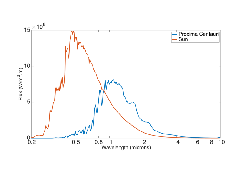
Figure 1: Top of atmosphere spectral flux for Earth (red) and ProC B (blue).

The Proxima Centauri stellar spectrum is from BT-Settl Rajpurohit et al. (2013) with $T_{\rm eff}=3000$ K, $g=1000$ m s^-2 and metallicity$=0.3$ dex, based on Schlaufman & Laughlin (2010). Correlated-$k$ absorption coefficients are recalculated using this stellar spectrum to weight wavelengths within the shortwave bands, and to cover the wider range of temperatures expected on ProC B. For simplicity we ignore the effects of atmospheric aerosols in all simulations, although tests with a simple representation of aerosol absorption and scattering did not lead to a significant difference in results. For the spectra and phase curves presented in Section 4 we additionally run short GCM simulations with high resolution spectral files containing 260 shortwave and 300 longwave bands that have been similarly adapted for ProC B from the original GA7 reference configurations.

Similar to Turbet et al. (2016), we use a flat, homogeneous surface at our inner boundary, but for simplicity choose a single layer ‘slab’ model based on Frierson et al. (2006). The heat-capacity of $10^{7}$ J K^-1 m^-2 is representative of a sea-surface with $2.4$ m mixed layer, although as all simulations are run to equilibrium, this choice does not affect the mean temperature, only the variability (capturing the diurnal cycle). We consider that simulations have reached equilibrium when the top-of-atmosphere is in radiative balance, the hydrological cycle (surface precipitation minus evaporation) is in balance and the stratospheric temperature is no longer evolving. We find that equilibrium is typically reached within 30 orbits, and show most diagnostics averaged over orbits 80-90 (sampled every model timestep). We retain water-like properties of the surface (even below $0\degree$C) allowing the roughness length to vary with windspeed, typically between $10^{-5}$ and $10^{-3}$ m. The emissivity of the surface is fixed at $0.985$ and the albedo varies with stellar zenith angle, ranging from $0.05$ at low zenith angles but reaching $0.5$ at very high zenith angles.

Table 2: Atmospheric parameters used in this study, for nitrogen dominated and Earth-like atmospheric compositions, where the Earth-like case contains further trace gases as in Earth’s current atmosphere.

$$\begin{array}[]{p{0.32\linewidth}|p{0.32\linewidth}|p{0.25\linewidth}}Parameter&nitrogen+trace CO${}_{2}$&Earth-like\\ \hline\cr$R$ / J\leavevmode\nobreak\ kg${}^{-1}$\leavevmode\nobreak\ K${}^{-1}$&$297$&$287.05$\\ $c_{p}$ / J\leavevmode\nobreak\ kg${}^{-1}$\leavevmode\nobreak\ K${}^{-1}$&$1039$&$1005$\\ CO${}_{2}$ MMR / kg\leavevmode\nobreak\ kg${}^{-1}$&\lx@intercol\hfil 5.941\cdot 10^{-4}\hfil\lx@intercol\\ O${}_{2}$ MMR / kg\leavevmode\nobreak\ kg${}^{-1}$&$0$&$0.2314$\\ \hbox{\multirowsetup O${}_{3}$ MMR / kg\leavevmode\nobreak\ kg${}^{-1}$}&\hbox{\multirowsetup$0$}&$2.4\cdot 10^{-8}$ (min)\\ &&$1.6\cdot 10^{-5}$ (max)\\ CH${}_{4}$ MMR / kg\leavevmode\nobreak\ kg${}^{-1}$&$0$&$1.0\cdot 10^{-7}$\\ N${}_{2}$O MMR / kg\leavevmode\nobreak\ kg${}^{-1}$&$0$&$4.9\cdot 10^{-7}$\\ \end{array}$$

All simulations have an atmosphere with a mean surface pressure of $10^{5}$ Pa, and we investigate two different atmospheric compositions, the relevant parameters for which are given in Table 2. These represent a nitrogen dominated atmosphere with trace amounts of CO₂, similar to that investigated by Turbet et al. (2016), and a more Earth-like atmospheric composition with significant oxygen and trace amounts of other radiatively important gases. Our motivation here is to explore the possible climate and observable differences that would exist on a planet that did support complex life Lenton & Watson (2011). The values for the gases are taken from present day Earth, and are globally uniform with the exception of ozone, for which we apply an Earth-like distribution, with highest values in the equatorial stratosphere, decreasing towards the poles and with much lower values in the troposphere. Whether an ozone layer could form and survive on ProC B is highly uncertain. Ozone formation requires radiation with wavelengths of $0.16-0.24\mu$m, which we expect to be in much shorter supply for ProC B, compared with Earth; see Figure 1 and Meadows et al. (2018). Meadows et al. (2018) also discuss that the likelihood of stellar flares destroying the ozone layer is quite high, and without it the chances of habitability are significantly reduced due to the large stellar fluxes at very short wavelengths ($<0.175\mu$m) received by ProC B. Essentially, in this work, our main aim is to investigate the response of an “Earth-like” atmosphere to the irradiation conditions (different spectrum and stellar flux patterns) characteristic of the ProC B system, so we refrain from removing individual gases which may actually be required for the planet to be habitable, or are potentially produced by an interaction of life with the atmosphere, such as ozone and methane Lenton & Watson (2011). A 3D model fully-consistent with the chemical composition is beyond the scope of the present work.

3 Results

In this section we discuss results from our simulations in two orbital configurations. Firstly, the assumption of a tidally-locked planet, and then a 3:2 spin-orbit resonance, both possible for such a planet as ProC B Ribas et al. (2016).

3.1 Tidally-locked case

We first consider the tidally-locked orbit with zero eccentricity. Figure 2 shows the surface temperature from our simulations. It is colder than the simulations of Turbet et al. (2016), with a maximum temperature on the day-side of $290$ K ($10$ K colder), and a minimum temperature in the cold-traps on the night-side of $150$ K, ($50$ K colder, informed by their figures). There are several reasons for these differences which we will explore.

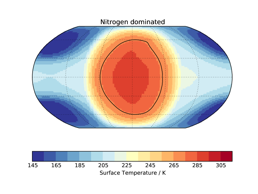
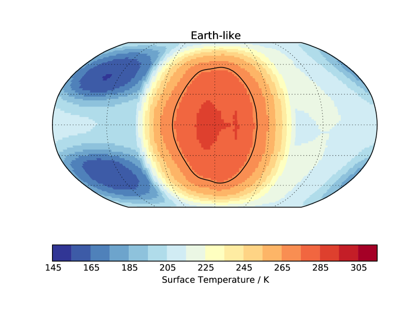
Figure 2: 10 orbit mean surface temperature (coloured) with the mean $0\degree$C contour, for the tidally-locked nitrogen dominated and Earth-like atmospheric compositions.

Firstly, we adopt a stellar radiation at the top of the atmosphere which is $70$ W m^-2 lower than Turbet et al. (2016), as discussed in Section 2, and so will inevitably be colder. We have tested our model with an incoming stellar flux consistent with that used by Turbet et al. (2016), and find that it increases the mean surface temperature by $5$ K across the planet (slightly less on the day-side and up to $10$ K in the cold-traps on the night side) which, critically, is still cooler than that found by Turbet et al. (2016). This increase is approximately two-thirds of that found for Earth ($4$ K for $45$ W m^-2 additional solar flux, Andrews et al., 2012), demonstrating that the sensitivity of planetary temperatures to changes in the stellar flux received by ProC B is quite low, meaning it potentially remains habitable over a larger range of orbital radii than e.g. Earth. This is likely to be due to a combination of the tidal locking and stellar spectrum. For example, changes in low cloud and ice amounts that contribute to a strong shortwave feedback on Earth are ineffective in this configuration as low clouds and ice are found largely on the night side of the planet.

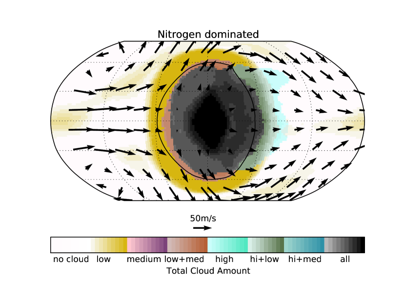
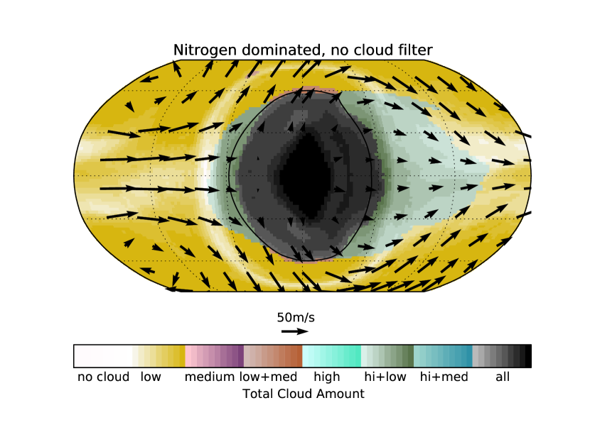
Figure 3: 10 orbit mean cloud cover (coloured) with the mean $0\degree$C surface temperature contour and wind-vectors at $8.5$ km, for the nitrogen dominated tidally-locked simulations, with and without filtering of optically thin cloud. Within each altitude range (low ¡ $2$ km ¡ medium ¡ $5.5$ km ¡ high) the cloud cover is given by the maximum cloud fraction ($\in[0,1]$) on any model level. If only one type of cloud is present, the colourbar shows that fraction, with a contour interval of $0.1$. If more than one type of cloud is present, the colourbar shows the average of the two or three cloud types present, again with colourbar interval of $0.1$.

On the day-side, cloud cover could be a contributing factor in keeping the surface cooler in our simulations. As shown in Figure 3, the day-side of the planet is completely covered in cloud, due to the strong stellar heating driving convection and cloud formation. This makes the albedo of the day-side quite high ($\approx 0.35$), reflecting a significant fraction of the incoming radiation back to space, similar to simulations presented by Yang et al. (2013).

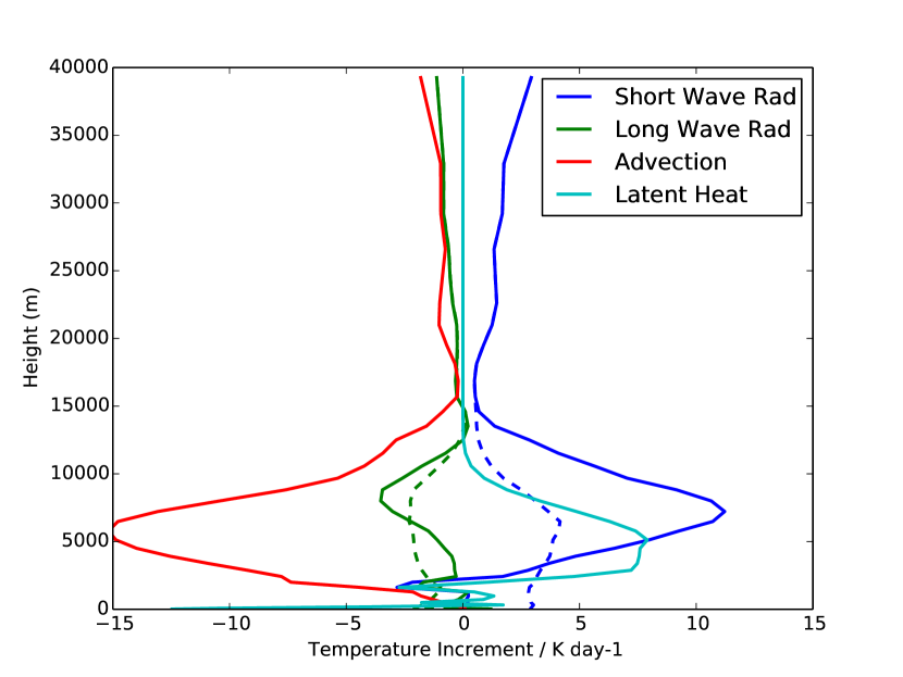
Figure 4: 10 orbit mean heating profiles from the sub-stellar point on the day-side of the nitrogen dominated tidally-locked simulation for the main physical processes. The dashed lines show the clear-sky heating from the radiation components.

Furthermore, the radiative heating of the thick cloud layer which forms is very high ($>10$ K day^-1, Fig. 4). It is possible that the combination of these two effects is greater in our model (driven by differences in our cloud and convection schemes, discussed later in this section), simply resulting in less radiation reaching the planet surface, and therefore a cooler surface temperature. However, the cooler day-side temperature may actually be linked to the temperature on the night-side, via the mechanisms described in Yang & Abbot (2014). They argue that the free tropospheric temperature should be horizontally uniform, due to the global-scale Walker circulation that exists on a tidally-locked planet Showman et al. (2013), and efficient redistribution of heat by the equatorial superrotating jet Showman & Polvani (2011). Figure 5 shows this to be true in our simulations, and the weak temperature gradient Pierrehumbert (1995) effectively implies that the temperature of the entire planet is controlled by the efficiency with which emission of longwave radiation to space can cool the night-side of the planet. Therefore, the fact that our night-side is so cold implies a very efficient night-side cooling mechanism which in turn suppresses the day-side temperatures.

The temperature on the night-side is cold due to the almost complete absence of cloud and very little water vapour. This allows the surface to continually radiate heat back to space, and cool dramatically. The only mechanism to balance this heat loss is transport from the day-side of the planet at higher levels within the atmosphere, followed by subsidence (where a layer of air descends and heats under compression) or sub-grid mixing to transport the heat down to the surface. Figure 5 shows profiles of temperature from the day- and night-side of the planet, demonstrating that the cooling is confined to the lowest $3$ km of the atmosphere, with the most extreme cooling ($30$ K) in the lowest $1$ km. We speculate that it is this near surface cooling which differs between our model and that of Turbet et al. (2016), as our temperature at $500$ m altitude appears very similar to their surface temperature (not shown).

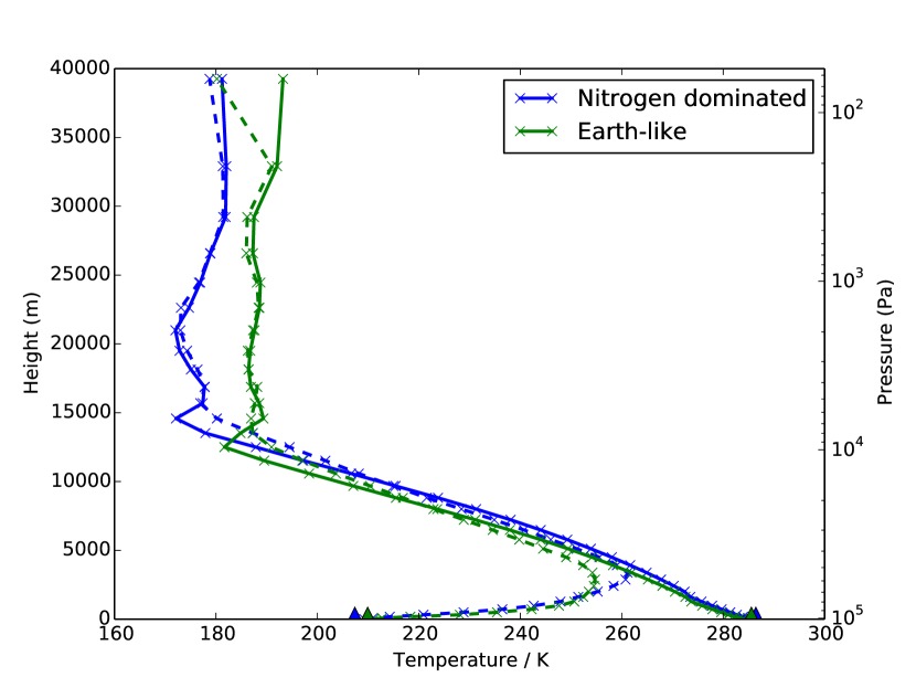
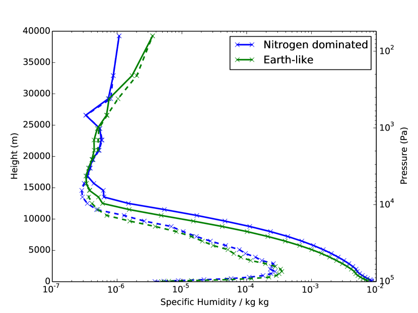
Figure 5: 10 orbit mean profiles of temperature and water vapour (top and bottom panels, respectively), from the sub-stellar point on the day-side of the tidally-locked planet (solid), and its antipode (dashed). Filled triangles show the surface temperature, and crosses indicate the position of the model-levels.

There are several possible reasons for the surface temperature differences between our model and that of Turbet et al. (2016). Firstly, the water-vapour profile could play a role. The night-side is dry because its only real source of water vapour is transport from the day-side, but this transport typically happens at high levels within the atmosphere, where the air is very dry due to the efficiency with which the deep convection precipitates water. This is likely to be a key uncertainty and potential reason for differences between simulations, as the convective parametrizations are very different – a simple adjustment scheme Manabe & Wetherald (1967) used in Turbet et al. (2016) versus a mass-flux based transport scheme (based on Gregory & Rowntree, 1990, but with significant improvements) used here. Secondly, model-resolution and the parametrization of turbulent mixing in the stable atmosphere are hugely important. How much sub-grid mixing atmospheric models should apply in stable regions is still a topic of research in the GCM community Holtslag et al. (2013), with many GCMs often applying more mixing than observations or theory would suggest. The UM uses a minimal amount of mixing in stable regions, which results in very little transport of heat down to the surface by sub-grid processes, and relies on the subsidence resolved on the model grid to warm the surface, which is also very weak in our lowest model level ($20$ m above the surface). Tests with increased mixing can produce a $20$ K increase in surface temperature, and also significantly alter the positions of the cold-traps.

The absence of cloud is another possible reason for surface temperature differences; results presented in Yang et al. (2013) showed uniform low level cloud cover on the night-side of a tidally-locked planet, which could help to insulate the surface and keep it warm. However, what cloud there is on the night-side of our model has such low water content that it is optically very thin and has almost no effect on the radiation budget. In Figure 3, we show the same cloud cover field, but in the bottom panel we show cloud as any grid-box with condensed water, whereas in the top panel we only consider a grid-box to be cloudy if that cloud is radiatively important (e.g. it would be visible to the human eye). This is done by filtering all cloud with an optical depth $<0.01$ from the diagnostic. This shows that whilst the cloud cover can appear quite extensive on the night-side, the cloud is actually radiatively unimportant. Finally, our model is lacking a representation of condensible CO₂, which could be an important contributor to the radiative balance of the night-side, both if vapour CO₂ concentrations are locally increased on the night-side, or CO₂ clouds are present. However, for the concentrations of CO₂ considered here, condensation would occur at $\approx 125$ K near the surface, and therefore condensation of CO₂ would appear unlikely, even in the cold-traps. We note that our surface temperature on the night-side appears very similar to the dry case of Turbet et al. (2016), and that our night-side surface temperature appears to match the very cold results given by the simple model of Yang & Abbot (2014) better than their GCM results which kept the surface warmer.

The temperature and water-vapour profiles shown in Figure 5 appear in good agreement with Turbet et al. (2016). Figure 4 shows that there is significant shortwave heating in the stratosphere, a result of shortwave absorption by CO₂ in our model, which is happening longward of $2\mu$m. This is a feature of Proxima Centauri’s spectrum (Fig 1), and would not happen on solar system planets due to the much lower flux at this wavelength from the Sun. The heating is balanced by longwave cooling from the CO₂ and water vapour, and transport of heat to the night-side of the planet. Figure 4 shows that heat transport is the dominant mechanism of heat-loss from the day-side throughout the atmosphere, and this heat is transported to the night-side where it is the only heat source and balanced by longwave cooling.

The differences due to atmospheric composition are generally quite small within the troposphere. The Earth-like composition has a similar surface temperature on the day-side, and slightly warmer surface temperature on the night-side, particularly in the cold traps. Consistent with Yang & Abbot (2014), this difference is primarily driven by additional heat on the day-side of the planet being transported to the night-side, effectively stabilising the temperature of the day-side and increasing the temperature of the night-side. Most other fields are very similar and not shown for brevity. There are however significant differences in the stratosphere (Fig. 5). The stratosphere is warmer, and this is predominantly driven by the ozone layer. However, the warming created is much less than on Earth, because there is very little radiative flux in the region which ozone absorbs ($0.2-0.32\mu$m). The stratosphere is also wetter, and this is a direct consequence of water vapour production by methane oxidation in this configuration. This is achieved via a simple parametrization Untch & Simmons (1998), common in many GCMs, that increases stratospheric water vapour in proportion to the assumed methane mixing ratio and observed balance between water vapour and methane in Earth’s stratosphere.

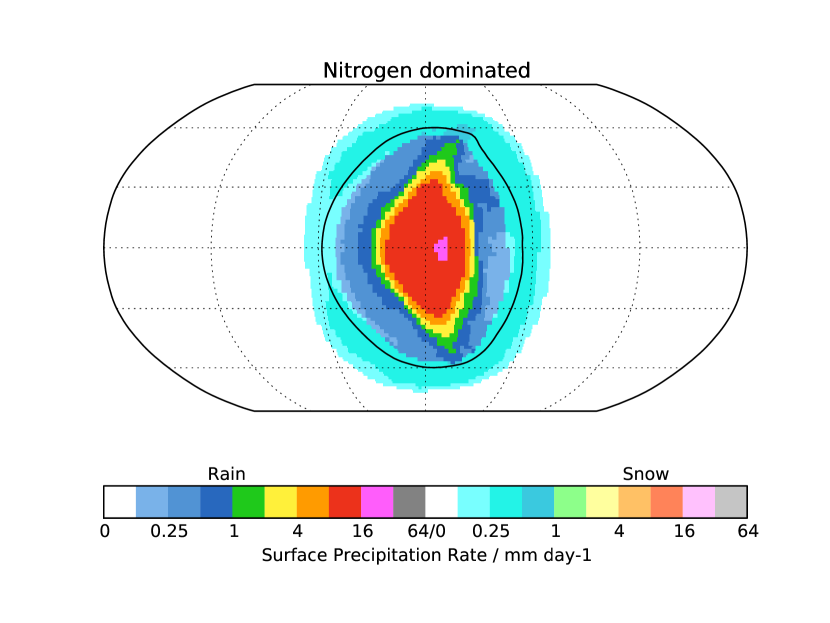
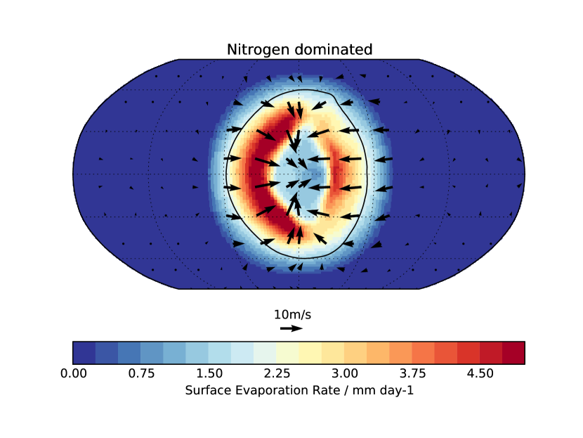
Figure 6: 10 orbit mean surface precipitation and evaporation rates (coloured) with the mean $0\degree$C surface temperature contour and wind-vectors at $10$ m, for the tidally-locked nitrogen dominated atmospheric composition.

Figure 6 shows the surface precipitation rate, showing intense precipitation at, and slightly down-wind of, the sub-stellar point on the day-side of the planet, decreasing in intensity radially from this point. The most intense precipitation comes from deep convection above this point, with the depth of the convection gradually reducing with radial distance, through the congestus regime (i.e. convection that terminates in the mid-troposphere) and ultimately shallow convection near the edge of the cloud layer. This can be seen quite clearly in Figure 3, with cloud height transitioning from low+medium+high, to low+medium, to low at increasing distances from the sub-stellar point. In many ways the transition is similar to the transition from shallow to deep convection in the trade regions of Earth. High cloud detrained into the anvils of convection is advected downstream by the equatorial jet, giving rise to a distinct asymmetry in the high cloud cover. The phase of the precipitation switches to snow in a ring around the edge of the day-side where the temperature drops below freezing, although it is interesting to note that the dominant phase of the precipitation is still snow even for surface temperatures above freezing. This is due to a combination of the time taken for the precipitation (which forms in the ice phase) to melt at temperatures above freezing, and the fact that near surface winds are predominantly orientated radially inwards near the surface, which advects the snow into warmer regions.

One interesting difference from tropical circulation on Earth is that the strong radiative heating of both the clear sky and cloud tops effectively stabilises the upper atmosphere. This keeps the majority of the convection quite low within the atmosphere, and only allows the most intense events to reach the tropopause level. The surface precipitation is therefore approximately $50$% convective, with the remainder being large-scale precipitation coming from the extensive high-level cloud and driven by a large-scale ascent on the day-side of the planet. This ascent is driven by convergence, similar to that shown in Figure 6, occurring throughout the lowest few kilometres of the atmosphere. This results in a latent heating profile below $4$ km in Figure 4, which is near-zero due to averaging of intermittent convective events, which generate strong heating, and persistent rain falling from the high-level cloud and evaporating, cooling the air (in contrast to Earth).

Figure 6 also shows the surface evaporation rate, and demonstrates that the moisture source for the heaviest precipitation is not local. The surface moisture flux is very low at the sub-stellar point, and highest in a ring surrounding this. This inflow region to the deep convection is where the surface winds are strongest, driving a strong surface latent heat flux. The near surface flow moistens and carries this water vapour into the central sub-stellar point, before being forced upwards in the deep convection and precipitating out. Combined with Figure 6, we can infer that most of the hydrological cycle on a planet like this occurs in the region where liquid water is present at the surface, i.e. the circulation does not rely strongly on evaporation from regions where the surface is likely to be frozen. Neither does the circulation transport large amounts of water vapour into these regions, and so this configuration could be stable for long periods if the return flow of water into the warm region (via glaciers or sub-surface oceans) can match the weak atmospheric transport out of this region.

3.2 3:2 resonance

We consider now the possibility of asynchronous rotation in a 3:2 spin-orbit resonance. In this case we model an atmosphere dominated by nitrogen, as in Section  3, and do not consider an Earth-like composition, as the differences between the two were found to be small for the tidally-locked case.

Figure 7 shows the results from a circular orbit, and unlike Turbet et al. (2016) we find that the mean surface temperature is above $0\degree$C in a narrow equatorial band, with seasonal maximum temperatures above freezing extending to $35\degree$ in latitude north and south of the equator. There are several possible explanations for this. Firstly, the greenhouse effect may be stronger, implying that more water vapour is retained in the atmosphere in our simulations (as we know that CO₂ concentrations are similar). Secondly, the meridional heat transport may be weaker in our simulations, as it appears (by comparison to their figures) that our polar regions may be colder. Finally, the lack of an interactive ice-albedo at our surface may be important here. To test this, we set the surface albedo to $0.27$ everywhere, to be representative of an ice covered surface, based on the mean spectral albedo of the surface ice/snow cover calculated by Turbet et al. (2016). We find that in this state, the mean surface temperature does fall below $0\degree$C everywhere (not shown), although seasonal maximums above freezing are still retained. Therefore, although the mean temperature of the planet is higher in our simulations, it is still likely that this configuration would fall into a snowball state.

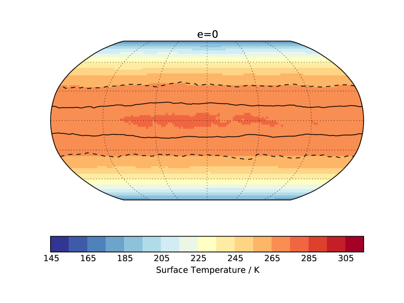
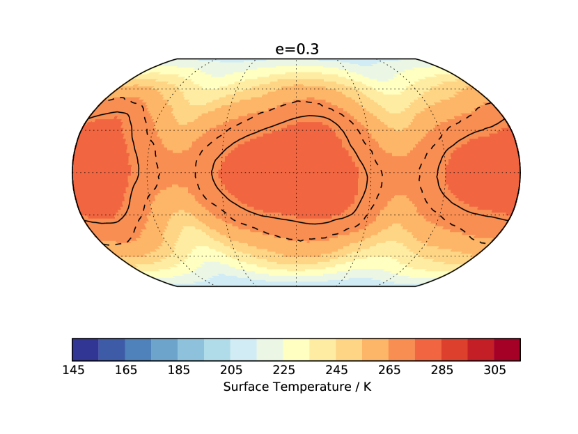
Figure 7: 10 orbit mean surface temperature (coloured) with the mean (solid) and seasonal maximum (dashed) $0\degree$C contours, for the circular and eccentric orbits in a 3:2 resonance.

The chance of a planet existing in a resonant orbit with zero eccentricity is small Goldreich & Peale (1966) yet if ProC B is the only planet in the system, the eccentricity excited by $\alpha$ Centauri alone is likely to be $\approx 0.1$ Ribas et al. (2016). Current observations can not exclude a further planet(s) orbiting exterior to ProC B, and are consistent with an eccentricity as large as $0.35$ (Anglada-Escude et al., 2016), with the most likely estimate $0.25$ Brown (2017). Therefore we have run a range of simulations assuming a 3:2 resonant orbit but with eccentricities varying from zero to $0.3$, and focus discussion on the most eccentric case. With increasing eccentricity, the region where the mean surface temperature is above freezing becomes concentrated in two increasingly large patches, corresponding to the side of the planet which is facing the star at periastron on each orbit. Therefore, permanent liquid water could exist at the planet surface, and the potential for the planet to fall into a snowball state is greatly reduced.

In an eccentric orbit the stellar heating is concentrated in two hot-spots on opposite sides of the planet Dobrovolskis (2015), leading to large regions of the surface which are warmer than their surroundings. Figure 8 shows how the incoming top-of-atmosphere shortwave radiation varies between orbits for the circular and eccentric configurations. The increase in radiation as the eccentric orbit approaches periastron is much greater than the decrease in radiation as it approaches apoastron, resulting in a significant increase in the mean stellar flux over large regions of the planet. This, combined with the fact that the total equatorial radiation is increased by $40$ W m^-2 (the global mean is closer to $30$ W m^-2), keeps the hot-spots well above freezing, with mean temperatures above $280$ K and seasonal maximums of $295$ K. The global mean temperature however only rises by $4$ K, which for an effective increase in stellar flux of $120$ W m^-2 ($30$ multiplied by the surface-area to disc ratio of $4$) implies an even lower sensitivity of this orbital state to changes in the stellar flux than in the tidally-locked case. We find that the sensitivity to the stellar flux changes for a 3:2 resonance in a circular orbit is approximately equal to the tidally-locked case ($5$ K of warming for $70$ W m^-2 additional flux), implying that the lower sensitivity is due to the eccentricity of the orbit – the high cloud cover formed over the hot-spot regions (Fig. 10) increases the reflected shortwave radiation, increasing the planetary albedo. This shows, similar to Bolmont et al. (2016), that the mean flux approximation is poor for this eccentric orbit.

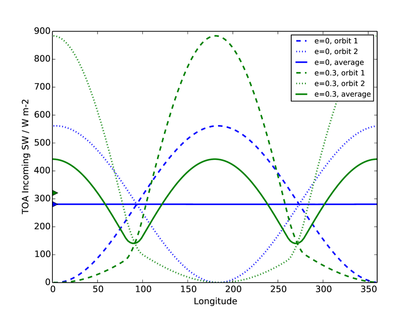
Figure 8: Equatorial cross-section of the top-of-atmosphere incoming shortwave radiation, meaned over a single orbit, showing two consecutive orbits for the circular and eccentric configurations (dashed and dotted) in a 3:2 resonance. Also shown is the mean of these two consecutive orbits (solid), and the zonal mean of this (filled triangles).

To test the possibility of the planet falling into a snowball state in this orbital configuration, we again set the surface albedo to be $0.27$ everywhere, to represent a snow/ice covered surface. This represents the most extreme scenario possible, as it would imply that any liquid water at the surface has managed to freeze during the night, which only lasts $12$ Earth days. Figure 9 shows that even in this case, the mean surface temperature remains above zero (and in fact the minimum only just reaches freezing), implying that the chance of persistent ice formation in these regions is small and the planet is unlikely to snowball. Additional tests with intermediate values of orbital eccentricity allow us to estimate that an eccentricity of $\approx 0.1$ would be required to maintain liquid water at the surface and prevent this configuration falling into a snowball state. The intermediate eccentricity simulations display many features of the most eccentric orbit presented here, i.e. the formation of hot-spot regions, but their strength obviously increases with increasing eccentricity.

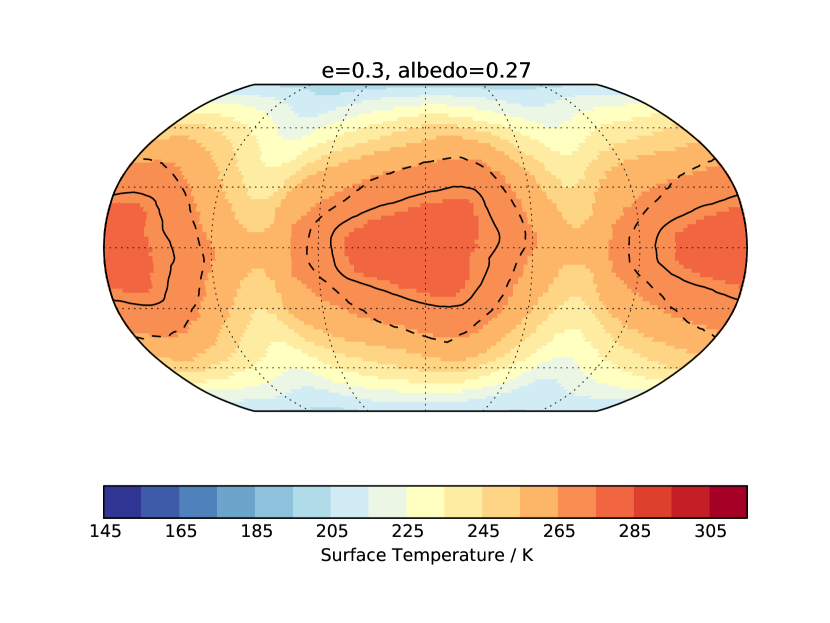
Figure 9: 10 orbit mean surface temperature (coloured) with the mean (solid) and seasonal maximum (dashed) $0\degree$C contours, for the eccentric orbit in a 3:2 resonance with surface albedo representative of an ice/snow covered surface.

GCM studies of resonant orbits with eccentricity appear to be rare, and therefore we document here what this climate might look like in the most eccentric case. In many respects, it appears similar to the tidally-locked case presented in Section 3.1, except now with two hot-spots on opposite sides of the planet and a much reduced planetary area in which water would be frozen. There are no significant cold-traps, with the polar regions being the coldest area with surface temperatures just above $200$ K, not too dissimilar from Earth (surface temperatures in Antarctica are typically $210$ K). As this simulation contains no ocean circulation, we speculate that if this were included, it could transport more heat away from the hot-spots and further warm the cold regions.

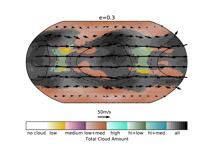
Figure 10: 10 orbit mean cloud cover (coloured) with the mean (solid) and seasonal maximum (dashed) $0\degree$C surface temperature contours and wind-vectors at $8.5$ km, for the eccentric orbit in a 3:2 resonance. Low cloud is below $2$ km and high cloud is above $5.5$ km, see Fig. 3 for more details.

Figures 10 and 11 show that the hot-spots are dominated by deep convective cloud with heavy precipitation. The upper-level circulation appears to be dominated by a zonal jet covering most of the planet, and similar to the tidally-locked case, this acts to advect the convective anvils downstream into the cold regions of the planet, almost completely encircling the planet, and maintain a horizontally uniform temperature in the free troposphere of the planet (not shown). Most of the planet is covered in low and mid-level cloud, apart from sub-tropical regions downstream of each hot-spot where there is only low-level cloud, similar to persistent stratocumulus decks on Earth. These cloud decks form in the regions of large-scale subsidence, compensating for the large-scale ascent which occurs in the hot-spot regions.

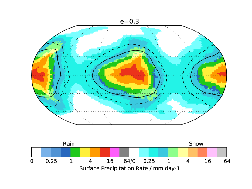
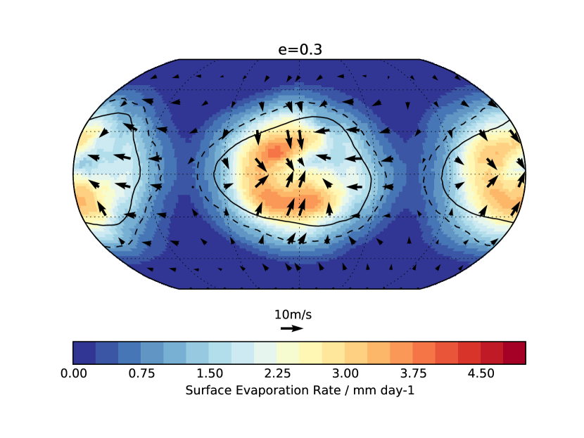
Figure 11: 10 orbit mean surface precipitation and evaporation rates (coloured) with the mean (solid) and seasonal maximum (dashed) $0\degree$C surface temperature contours and wind-vectors at $10$ m, for the eccentric orbit in a 3:2 resonance.

The cloud is thick enough to precipitate around the entire equatorial belt, and reaches $60\degree$ north/south at the central longitude of the hot-spots. Similar to the tidally-locked case, the heaviest precipitation is downstream of the peak stellar irradiation, due to the strong zonal winds. The winds also shift polewards at this location, which creates two limbs of enhanced precipitation stretching polewards downstream of the hot-spot. The low level flow is generally equatorwards (Fig. 11), and this is strongest in the warm regions, leaving weak winds in the colder subtropical regions, ideal for the formation of non-precipitating low cloud.

Figure 11 also shows the surface evaporation rate, which unlike the tidally-locked case is not strongly confined to a region surrounding the deepest convection, but instead appears quite local to the precipitation. It is predominantly to the upstream side of the heaviest precipitation, and this is due to the lower cloud cover in this region allowing more stellar radiation to reach the surface. The hydrological cycle of each hot-spot appears reasonably self contained, with the possibility that there will only be limited exchanges of water between the opposing sides of the planet. Similar to the tidally-locked case, the hydrological cycle is also largely confined within regions where surface liquid water is present, suggesting that this configuration could be stable for long periods.

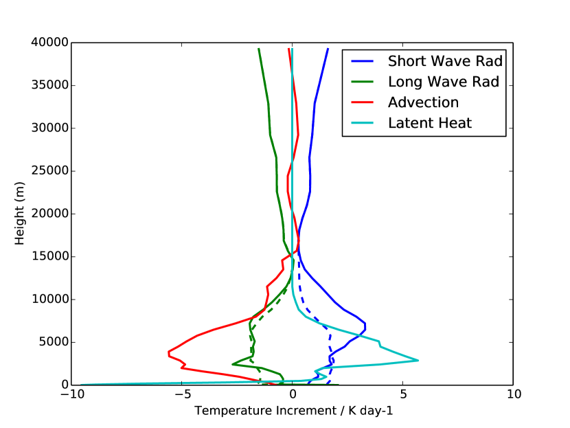
Figure 12: 10 orbit mean heating profiles from the main physical processes, at the centre of one of the hot-spot regions of the planet in an eccentric orbit with 3:2 resonance. The dashed lines show the clear-sky heating from the radiation components.

Whilst there are many similarities in the resultant climate between the tidally-locked case and the hot-spots on the 3:2 eccentric case, the mechanisms which create them do show some differences. The 3:2 case is more similar to Earth in its heating profiles (Fig. 12), with latent heating due to convection dominating over shortwave heating throughout the lower-to-mid troposphere. The magnitude of the shortwave heating is much lower than in the tidally-locked case, although still significantly higher than on Earth McFarlane et al. (2007), and this does not act to stabilise the upper troposphere and suppress the convection. The resulting climate therefore has deep convection mixing throughout the troposphere during the day, and the majority of the precipitation is convective in this simulation. It therefore presents a somewhat intermediate solution between the tidally-locked case and Earth. The fact that the whole planet is irradiated at some point during the orbit means there is no stratospheric transport of heat from day to night, with the stratospheric heating and cooling being entirely radiative in nature.

4 Spectra and Phase Curves

We have produced individual, high-resolution reflection (shortwave) and emission (longwave) spectra, as well as reflection/emission as a function of orbital phase angle within wavelength ‘bins’. Turbet et al. (2016) include a full discussion on the possibility of detecting this planet with current and upcoming instrumentation, so we do not repeat this here. Instead, we present our simulated emissions and discuss their key features, and differences with Turbet et al. (2016).

We obtain the top-of-atmosphere flux directly from our GCM simulation, as done by Turbet et al. (2016), where the wavelength resolution is defined by the radiative transfer calculation in the GCM. The radiative transfer calculation used in our GCM, and that of Turbet et al. (2016), adopts a correlated-$k$ approach, effectively dividing the radiation calculation into bands. The bands themselves, and details of the correlated-$k$ calculation are essentially set to optimise the speed of the calculation while preserving an accurate heating rate (see discussion in Amundsen et al., 2014, 2016). Therefore, spectral resolution is sacrificed.

To mitigate this effect, we run the model for a single orbit with a much greater number of bands (260 shortwave and 300 longwave), which greatly increases the spectral resolution. The top-of-atmosphere flux is output every two hours, or approximately 144 times per orbit for ProC B. From these simulations we compute the emission and reflection spectra, as well as the reflection/emission as a function of time and orbital phase. The outgoing flux at the top of the model atmosphere is translated to the flux seen at a distant observer by taking the component of the radiance (assumed to be isotropic) in the direction of the observer and then summing over the solid angle subtended by each grid point over the planetary disc.

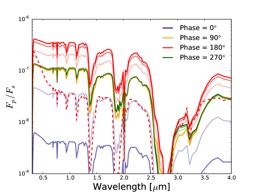
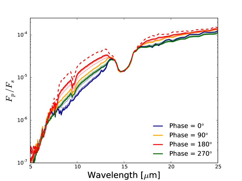
Figure 13: Reflectance (left) and emission (right) spectra for the tidally-locked Earth-like case at four points in the planets orbit. Spectra for observer inclinations of 90$\degree$, 60$\degree$ and 30$\degree$ are shown in progressively fainter lines. For comparison, we include the clear-sky flux for the phase = 180$\degree$ spectrum with an observer inclination of 90$\degree$ (dashed), which highlights the importance of the role of clouds in the shortwave spectrum. The sharp drop-off in the flux ratio at short wavelengths is due to ozone absorption

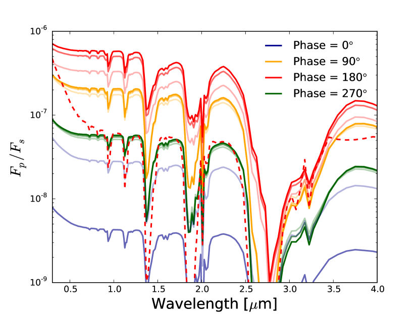
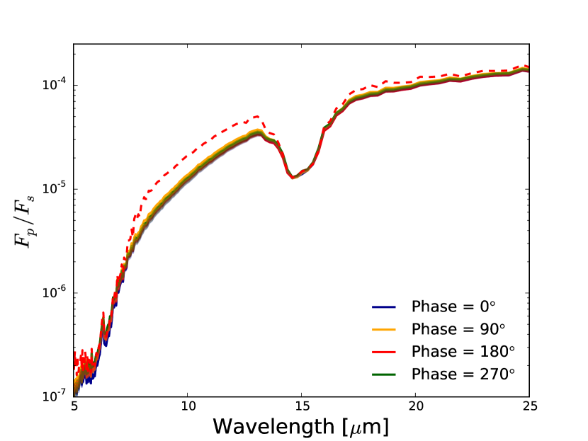
Figure 14: As Figure 13, but for the 3:2 resonance nitrogen-dominated case, and we show the clear-sky flux for phase = 180$\degree$.

Figure 13 shows the reflection (shortwave) and emission (longwave) planet-star flux ratio for the tidally-locked case with an Earth-like atmosphere. The contrast between planet and star ($F_{p}/F_{s}$) is shown as a function of wavelength (in $\mu$m) for a range of orbital phases and inclinations ($i$). We follow the approach of Turbet et al. (2016), where an inclination $i$ = 90$\degree$ represents the case where the observer is oriented perpendicular to the orbital axis. Additionally, an example for the “clear-sky” emission is shown (dashed line), ignoring the radiative effect of the cloud in the simulated observable. These figures are comparable to their counterparts in Turbet et al. (2016) (Figures 8 and 12). We have separated the long and shortwave flux (meaning our contrast is underestimated for the shortwave at wavelengths longer than 3.5$\mu$m, as is the case in Turbet et al., 2016), and adopted a radius of 1.1 R_⊕. The differences will then be caused by the direct differences in the top of atmosphere fluxes obtained in our simulations, and the resolution of our emission calculation.

In the shortwave case, our spectrum generally compares well with that of Turbet et al. (2016), showing similar trends and features, particularly the absorption features from water and CO₂. However, we find an overall larger $F_{p}/F_{s}$ ratio (e.g. by a factor of 2 between 2.0 and 2.5 $\mu$m), which is likely to be the result of subtle differences in the quantity and distribution of clouds, which have a significant influence on the shortwave reflection, as shown by the clear-sky spectrum, also shown in Figure 13. Our inclusion of the full complement of Earth’s trace gases along with increased resolution reveals more spectral features, especially at short wavelengths, but the overall shape and magnitude of the contrasts compare well to Turbet et al. (2016). Our inclusion of oxygen leads to the absorption feature at 0.76 $\mu$m, and an ozone layer to the absorption at ultra-violet wavelengths. As discussed previously, the presence of an ozone layer in the atmosphere of ProC B is very uncertain. However, our aim here is to explore how a truly Earth-like atmosphere would respond to the irradiation received by ProC B. Comparing the shortwave contrast from our outputs at $\phi$=180$\degree$ with (solid line) and without (dashed line) clouds we can see that the cloud acts to increase the shortwave contrast due to scattering and slightly ‘mute’ the absorption features.

Figure 13 also shows a reasonable agreement of the overall shape and magnitude of our longwave flux ratio with that of Turbet et al. (2016). As for the shortwave case our increased resolution reveals additional features in the spectrum. The main difference here is the absorption feature at $9.6\mu$m due to the presence of ozone, which is not included in the model of Turbet et al. (2016).

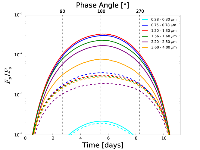
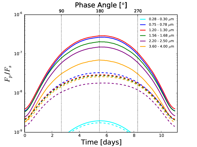
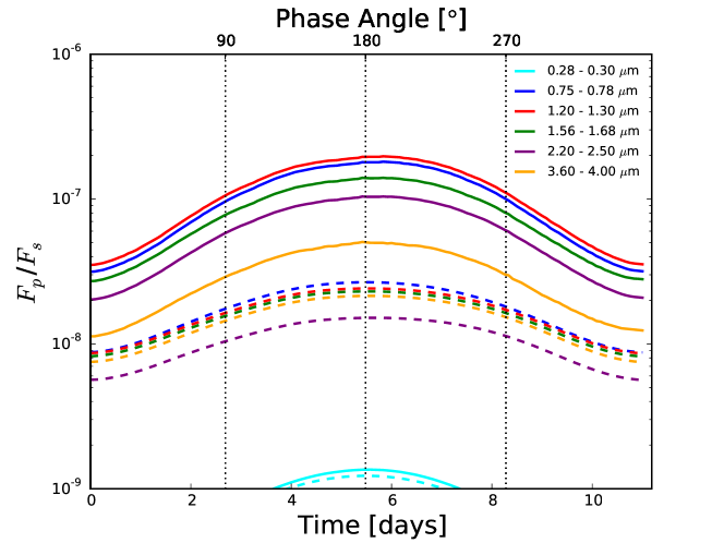
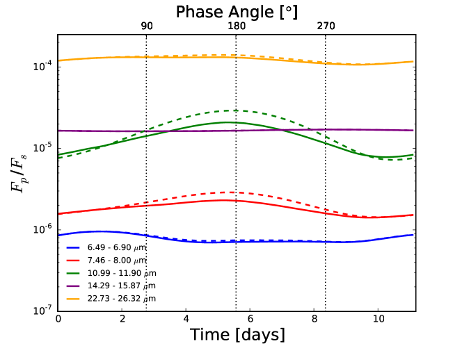
Figure 15: Reflectance phase curves for observer inclinations of (from top to second from bottom) 90$\degree$, 60$\degree$ and 30$\degree$ and the emission phase curve for an observer inclination of 60$\degree$ (bottom) for the tidally-locked Earth-like case. Phase curves are shown for wavelength ranges closely matching those of Turbet et al. (2016) for comparison. Clear-sky fluxes are represented in dashed lines to highlight the role of clouds, which generally increase the shortwave planetary flux but have much more subtle effects for the longwave flux. The emission phase curves show very little variation with observer inclination, hence we only show the $i$ = 60$\degree$ case for brevity. Note that we find a very small flux ratio in the 0.28-0.30$\mu$m region, due to ozone absorption.

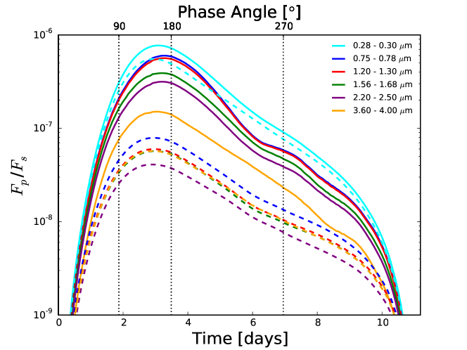
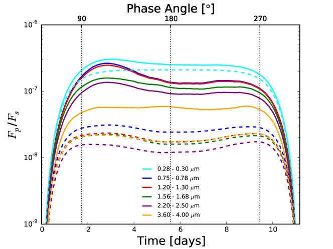
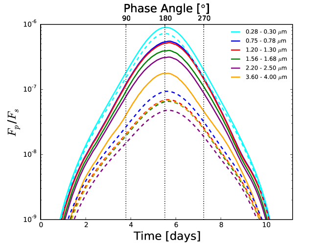
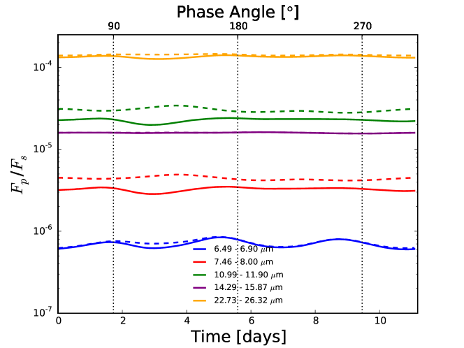
Figure 16: Reflectance phase curves for observer longitudes such that periastron is at 102$\degree$, 0$\degree$ and 180$\degree$ phase angle(from top to second from bottom), and the emission phase curve for an observer such that periastron is at 0$\degree$ phase (bottom) for the 3:2 resonance nitrogen-dominated case. Lines are as in Fig. 15. We only show one orbit, as due to the symmetry of the planetary climate, the subsequent orbit produces almost identical phase curves. The emission phase curves show very little variation with observer longitude, hence we only show the view from behind periastron for brevity.

Figure 15 shows the emission as a function of orbital phase angle for the Earth-like, tidally-locked simulation, at three inclinations ($i$=30$\degree$, 60$\degree$ & 90$\degree$) for the shortwave and at only one inclination ($i$=60$\degree$) for the longwave (due to the invariance of the longwave phase curve with inclination). We do not adjust the radius (and therefore total planetary flux) with inclination using $R_{p}\propto(M_{min}/\sin i)^{0.27}$ as in Turbet et al. (2016), since to be fully consistent this would require running all climate simulations with an adjusted radius. Instead the phase curves represent an identical planet observed from different angles. As with Figure 13 the “clear-sky” contribution is also shown as a dashed line.

We generally find very good agreement with the results of Turbet et al. (2016). Of notable difference in the reflectance phase curves is the much reduced flux ratio in the 0.28–0.30 $\mu$m region, due to absorption by ozone which is not included in the model of Turbet et al. (2016), which means that our predicted flux contrast is two orders of magnitude smaller in this band. In addition, we find the largest flux ratio to be in the 1.20–1.30 $\mu$m band, in contrast to Turbet et al. (2016) who find the 0.75–0.78 $\mu$m band to possess the largest contrast (disregarding the previously discussed 0.28–0.30 $\mu$m band). We find the planetary flux in the 0.75–0.78 $\mu$m is depressed by the oxygen absorption line at 0.76 $\mu$m, which is not included in the model of Turbet et al. (2016). Our longwave emission phase curves also show very similar trends to Turbet et al. (2016). However, we find that the flux contrast in the bands 7.46–8.00 $\mu$m and 10.9–11.9 $\mu$m is a factor few lower in our model, likely due to the presence of additional absorption by trace gases (CH₄ and N₂O at 7.46–8.00 $\mu$m) and the cooler surface temperature.

In Figure 15 we also show the clear–sky flux, ignoring the radiative effects of clouds, to highlight the important role that clouds have on the magnitude of the reflectance phase curves. The high albedo of clouds results in increases to the planet-star flux ratio by an order of magnitude. On the other hand, clouds have a much more subtle direct impact on the longwave emission spectrum; though of course the temperature of the atmosphere/surface has been influenced by the presence of clouds, and so they have an important indirect effect on the longwave emission through the temperature.

Figure 14 shows the reflection and emission spectra for the nitrogen dominated atmosphere in the eccentric ($e=0.3$), 3:2 resonance orbit. The shortwave spectrum is very similar to the tidally-locked Earth-like case, though note the lack of ozone absorption at very short wavelengths; ozone and other trace species not being included in this model. The longwave spectrum is very insensitive to orbital phase and inclination, due to the horizontally uniform nature of this atmosphere, as opposed to the tidally-locked model. The spectrum is generally quite featureless except for the absorption feature due to CO₂ around 15 $\mu$m.

Figure 16 shows the emission as a function of orbital phase for the 3:2 spin-orbit nitrogen dominated model. The full repeating pattern should contain two complete orbits, but due to the symmetry of the planetary climate, each orbit produces a very similar phase curve, and therefore we only present a single orbit for clarity.

For the shortwave reflection, we find broadly similar results to those of the tidally-locked Earth-like case. However, in this case the phase curve is now strongly affected by the longitudinal position of the observer and eccentricity of the orbit. It is almost symmetric when viewed from periastron or apoastron, and any deviations from this are due to the atmospheric variability of the planet. For example, the peak flux contrast when viewed from periastron is at $\sim 120\degree$, and is due to reflection from the high, convectively generated cloud above the hot-spot, which was recently heated at periastron and has just appeared into view. There is no corresponding peak at $\sim 240\degree$ because although we are again seeing a hot-spot, this one has not been heated since periastron on the previous orbit, and so the convective cloud has decayed significantly. When viewed from the side, the planetary phase curves display a strong asymmetry. The most striking asymmetry is due to our choice to present the phase curve with a linear time axis (as a distant observer would see) rather than a linear phase angle axis, and is created by the apparent speedup and slowdown of the orbit near periastron and apoastron. However, the phase curve would still be asymmetric if plotted against a linear phase angle axis, due to the variation in stellar radiation received. For example, the peak clear-sky flux is at $\sim 150\degree$, and occurs because the peak radiation is received at periastron ($\sim 102\degree$), after which the radiation available for reflection is reducing whilst the visible area of the planet which is illuminated is increasing. The total flux is then offset slightly towards $180\degree$ from this, because there is a delay in the formation of the high, convectively generated clouds above the hot-spot after peak irradiation. The fact that features in the phase curves are dependent on the hydrological cycle, and the formation and evolution of water clouds, hints at an exciting opportunity to constrain this feature given sensitive enough observations.

The longwave phase curves show much less variation in the flux with orbital phase compared with the tidally-locked model. This is despite the fact that this model contains two hot spots due to the eccentricity ($e=0.3$) of the orbit, which are visible in the slight increase in contrast at $\sim 150\degree$. In fact, Figure 16 shows that the small variations in the flux due to these hot spots are damped out further by radiative effects of clouds, which appears as a reduction in the contrast over the hot-spot regions.

Overall, our simulated observations show many consistencies with those of Turbet et al. (2016), however, we also find a few important differences. Firstly, our calculations were performed in a much higher spectral resolution, allowing us to pick out specific absorption and emission features, in particular those associated with the gases vital to complex life on Earth, oxygen, ozone and CO₂. Secondly, we find that the shortwave phase curves show significant asymmetry in the 3:2 resonance model.

5 Conclusions

This paper has introduced the use of the Met Office Unified Model for Earth-like exoplanets. Using this GCM, we have been able to independently confirm results presented in Turbet et al. (2016), that ProC B is likely to be habitable for a range of orbital states and atmospheric compositions. Given the differences between the models, both in numerics (the fluid equations being solved and how this is done) and physical parametrizations (the processes included and level of complexity of the schemes), the level of agreement between the models is somewhat remarkable. Having this level of agreement from multiple GCMs is an important factor in the credibility of any results which are produced with a GCM, especially for cases such as ProC B where the observational constraints are (currently) very limited. As with many phenomena on Earth for which observations are limited, an alternative strategy to constrain the climate simulations could be more detailed modelling of specific parts of the climate system. For example, high-resolution convection resolving simulations of the sub-stellar point of the tidally-locked case would help to constrain the amount of cloud, precipitation, and export of moisture to the night side of the planet.

We have additionally shown in this paper that the range of orbital states for which ProC B may be habitable is larger than that proposed by Turbet et al. (2016). By use of a different, weaker, stellar flux, we have shown that the planet is still easily within a habitable orbit despite the known uncertainty in the luminosity of Proxima Centauri. This is a consequence of a particularly low sensitivity of planetary temperatures to changes in stellar flux received for ProC B. The inclusion of eccentricity to a 3:2 resonant orbital state was also shown to increase the habitability. This result could hold true for any planet near the outer (cold) limit of its habitability zone – including eccentricity in an orbit has the potential to increase the size of the habitable zone. Two factors combine to produce this effect. Firstly, the mean stellar flux will always be higher for an eccentric orbit, and secondly, for orbits in resonant states, a large increase in the stellar flux is received by fixed regions on the planet surface, which become permanent ‘hot-spots’. The circulation on planets in this configuration is not too dissimilar from the tidally locked case, with the number of hot-spots being set by the spin-orbit resonance. A planet in an eccentric orbit with a 2:1 resonance would have a single hot-spot and be very similar to the tidally-locked case. Whether eccentric orbits would reduce the habitable zone for planets near the inner (hot) limit is a matter for further study, and is likely to depend on other planetary factors, such as tidal heating discussed by Bolmont et al. (2017), and climate feedbacks such as the cloud feedbacks discussed by Yang et al. (2013).

There are obviously several ingredients missing from our analysis. We have neglected the presence of any land-surface, as we have no information what this may look like, but in considering the surface to be water covered we have additionally neglected any transport of heat by the oceans. Hu & Yang (2014) have recently investigated tidally-locked exoplanets with ocean circulation, demonstrating that the ocean acts to transport heat away from the sub-stellar point. If this were included in our simulations here, it is likely that the region where surface temperatures were above freezing would be increased in both the tidally-locked and 3:2 resonance cases, further reducing the potential for the 3:2 case to fall into a snowball regime. There is also the possibility that the location of continents and surface orography relative to the regions where surface temperatures were above freezing may significantly affect the planet’s climate and habitability.

We have also considered some more exotic chemical species (oxygen, ozone, methane etc) in our analysis, but have only specified them as globally invariant values. The reason for this is their importance in the evolution of complex life on Earth. The next logical step here is to couple a chemistry scheme to the atmospheric simulations, that allows these species to be formed, destroyed and transported by the atmospheric dynamics, and this would allow a much better estimation of the likely atmospheric composition.

We have generated, from our simulations, the emissions from the planet as a function of wavelength in high-resolution, allowing us to highlight signatures of several key (for complex life on Earth) gaseous species in the spectrum (oxygen, ozone and carbon dioxide). We have also generated emissions as a function of orbital phase angle from our simulations and find results largely consistent with Turbet et al. (2016). Overall our findings are similar, though our results present a higher spectral resolution, and show the importance of the observer longitude on the appearance of phase curves when the planet has an eccentric orbit.