The spatial statistics of turbulent dissipation rates
Abstract
We study the spatial statistics of velocity gradient volatility (i,e., the energy dissipation rate) in turbulent flow. We extend the Kolmogorov-Obukhov theory but also narrow its scope. The models are log normal, with verification from finely resolved large eddy and direct numerical simulations. They are parameterized by a mean and a covariance operator. Addressing applications to large eddy simulations, the mean and the covariance depend on the resolved scale solution. Removing this resolved scale dependence by a locally defined rescaling of the turbulent statistics yields a universal theory for the subgrid statistics, specifically for the mean and variance of turbulent fluctuations, i.e., the log of the energy dissipation rate . The variance of the velocity gradient statistics is found to be log normal, in accordance with Kolmogorov 1962. Rescaling by the resolved scale mean and variance removes the influence of the resolved scales on the subgrid scales, justifying conceptually the universality we observe. The universality is the basis of new power scaling laws. The new power laws, in turn, allow a simple parameterization of the mean and covariance of the subgrid rescaled dissipation rate, i.e., velocity gradient volatility. We treat the coarse grid resolved space-time location as a random variable. A restriction of the theory to a small range of unresolved but stochastically modelled scales is proposed, with renormalization group ideas offered to overcome this restriction.
I Introduction
The scaling law of Kolmogorov Kol41 , although simple, is among the deepest contributions to the understanding of turbulent flow. Turbulent flow is generally considered to be the major outstanding problem of classical physics. We propose new parameterized spatial statistics and scaling laws for turbulent fluctuations which extend ideas of the Kolmogorov 1962 (K62) theory but also narrow its scope. Verification is from comparison to Direct Numerical Simulation (DNS). Because we do not assume homogeneity or isotropy of the flow, the theory is applicable to the unresolved scales of Large Eddy Simulations (LES), and is a stochastic subgrid scale (SGS) model. A major contribution of the theory presented here is to capture SGS fluctuations, in addition to the means computed from traditional SGS theories.
We assume single fluid, constant density, incompressible flow, governed by the Navier-Stokes equation. The scalar dissipation rate is defined as
| (1) |
with the dynamic viscosity, the fluid velocity, and
| (2) |
the strain rate.
Properties of are fundamental to a number of deep theories of turbulence, including notions of turbulent intensity, turbulent intermittancy Sre04 , corrections to the Kolmogorov 5/3 exponent and scaling laws for velocity moments. The analysis of has been applied to turbulent diffusion, short distance asymptotics for the velocity two point correlation function, and prediction of a fractal or multifractal spatial distribution of regions of high turbulent intensity, with the turbulent regions concentrated in a fractal set of dimension Cho94 . Scaling laws for wall bounded turbulence (a topic not addressed here) are discussed in BarCho98 . There is an extensive literature on the above topics, which we do not attempt to document in this article. See the survey article Jou97 for elaborations and further references. Kolmogorov Kol62 and Obukhov Obu62 conjectured that obeys a lognormal distribution at sufficiently high Reynolds numbers.
Our main results are new scaling law for the mean and covariance of , which we designate as turbulent intensity. The scaling laws originate in a universality principle, of the mean and the variance of for inertial degrees of freedom. The connection between universality, which would seem to require isotropic homogeneous turbulence, and subgrid scales of LES, which can be very far from homogeneous or isotropic is one of our central results. Depending on the local properties of the resolved scales of turbulence, we introduce a rescaling of the turbulent statistics, and it is only after this rescaling that the subgrid scales of turbulence become universal. In fact, universality does have limits, in terms of the number of subgrid scales it can accommodate. In our numerical tests, we consider 3 levels of mesh refinement, that is a change of length scales by a factor of 8. For a large number of length scales, we have in mind a renormalization group methodology, with successive integration over smaller length scales, and a resetting of parameters using the (statistical) knowledge of the already integrated scales, a point of view to be elaborated in future work.
In Sec. II, we specify the simulation study used for verification of the theories proposed here. We define the statistics and the ensemble used. We show that has log normal statistics (and has normal statistics).
The spatial statistics for and are characterized by the mean and covariance of . We compare a coarsely gridded LES to a finely gridded LES or DNS. The fine grid extension of the coarse grid solution is of course unique and not stochastic, but we add statistics in the dependence of this extension on the resolved coarse grid cell from which it is derived. The statistics of the fine grid extension for depends on the coarsely gridded resolved solution.
A detailed analysis of the statistics is carried out in Fourier space, in Sec. III. The analysis uses the coarse grid resolved scales as a random varible, to define the statistical properties of the subgrid scales. Our premise is that the spatial aspects of this dependence are largely captured by a resolved scale variance and mean for . When the and dependency is removed from the refined solution extension by rescaling, the resulting statistics for , i.e., , is modeled as universal, with diagonal and subject to simple modeling assumptions, including new power laws, with only a few dimensionless parameters to govern its spatial statistics, all physically understandable. The power laws result from a universality principal for the rescaled statistics. These approximations are confirmed by the fine grid comparison.
II The spatial statistics
II.1 The simulation study
All verification tests are based on a series of coarse and finely gridded simulations. The finely gridded LES/DNS study has over two decades of resolution, with the coarsely gridded LES fraction of the solution varying with the simulation parameters. The coarsely gridded LES includes portions of the inertial range and has up to a decade of unresolved inertial range scales to which our modeling applies.
Our fine and coarse grid simulations are conducted with the code PouKolChe14 , using periodic boundary conditions and forced turbulence in a domain size , , with the viscosity (of air), . The mesh parameters for three simulations are given in Table 1. The resolved levels of turbulence in this numerical study are not extreme.
Let denote the coarse grid mesh size, and the fine grid mesh size, so that . As we are concerned with velocity gradients, which require two mesh cells as a minimum stencil size for their evaluation, we also introduce what we call the resolved coarse and fine grid mesh scales, with as the resolved coarse grid mesh and
| (3) |
Here the resolved fine grid level is , needed to evaluate the fine grid velocity gradients occurring in and .
| Fine grid | Fine and coarse | Re | Taylor Re | Kolmogorov |
| simulation | grid meshes | scale | ||
| DNS | and | 561 | 40 | |
| LES | and | 1577 | 67 | |
| LES | and | 2539 | 85 |
II.2 The statistical ensemble
As with turbulent flow in general, and can be regarded as random fields. In the LES context, and are known (deterministic) at the resolved scales, while their subgrid scale fluctuations can be modeled using spatial statistics. We write the fine grid resolved spatial mesh coordinate , where is the coarse grid resolved mesh portion of . As the resolved coarse mesh spacing is , spans all the coarse grid LES cells other than the last or finest of them. is the remainder, occurring in the fine but not the coarse LES grid resolution and also within the finest level of the LES simulation. There are then values and values. Note that mesh indices are missing, as we discuss resolved, not simulation mesh indices.
Our plan is to treat , regarded as a fiction of , as random, depending on the random variable . The natural domain for its mean and covariance and is the Hilbert space of subgrid functions, i.e., functions indexed by but restricted to a single resolved coarse grid cell and having mean zero there. is a vector in and is an positive definite matrix acting on .
The statistics are collected as an average over all the possible values of .
II.3 The log normal property
We present numerical evidence to support the hypothesis that the fine grid extension of the resolved defines a Gaussian random field, with the mean and covariance defined from averages of distinct resolved coarse grid cells.
The time dependent spatial average of has been tested for normality, see MonYag65 ; YeuPop89 ; PopChe90 and references cited there, based on experimental and DNS evidence. Our verification method to establish the Gaussian property is also based on DNS evidence. A multivariate random variable is Gaussian if its inner product with any fixed vector is univariate Gaussian. Here we consider, as representative choices, the fixed vectors defined by single DNS cell indices .
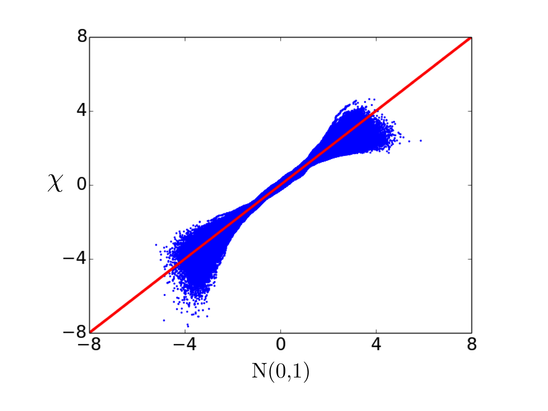
We use QQ plots to assess univariate normality. In these, the trial distribution is transformed first by a change of the independent variables to have zero mean and unit variance. Then we apply an inverse Gaussian change of trial distribution dependent variables, with the result compared to a unit slope straight line.
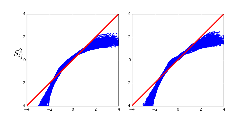
We create a single QQ plot by holding the fine grid mesh resolved cell indices fixed ( choices), and using the multiple values from the resolved coarse grid cells to form the ensemble. In Fig. 1 we superimpose all QQ plots for all choices of as typical tests of normality, demonstrating agreement to a Gaussian law up to , a range of agreement consistent with the 4% accuracy expected from the ensemble size.
II.4 The mean and covariance
The coarse grid resolved level variance of is basic to our rescaling strategy. At the level of each coarse grid resolved grid cell, the variance of is defined as
| (4) |
with the definitions .
Consider the fine grid values for the resolved coarse grid . As a normal random variable, the statistics of is characterized by its mean and its covariance. To obtain universal statistics, we rescale by subtracting the resolved coarse grid mean and dividing by the standard deviation defining . The mean of is
| (5) |
The universal, rescaled, statistics are the statistics of . We follow a similar definition for the covariance, of ,
| (6) |
where the overbar denotes averaging over all resolved coarse grid cells, namely
| (7) |
Furthermore, we will normalize by , the resolved scale variance, reducing the Reynolds number dependence of .
III Spatial statistics in Fourier space
We propose a Fourier space analysis for and . As these variables are independent of the resolved variables, they are, in this approximation, periodic within each resolved cell. Thus their Fourier transforms depend on the Fourier modes within a single resolved cell.
In preparing figures in this section, we present functions of , unless otherwise noted, after binning all values into bins labeled by the scalar wave number with 200 bins whose size is linear in .
III.1 in Fourier space
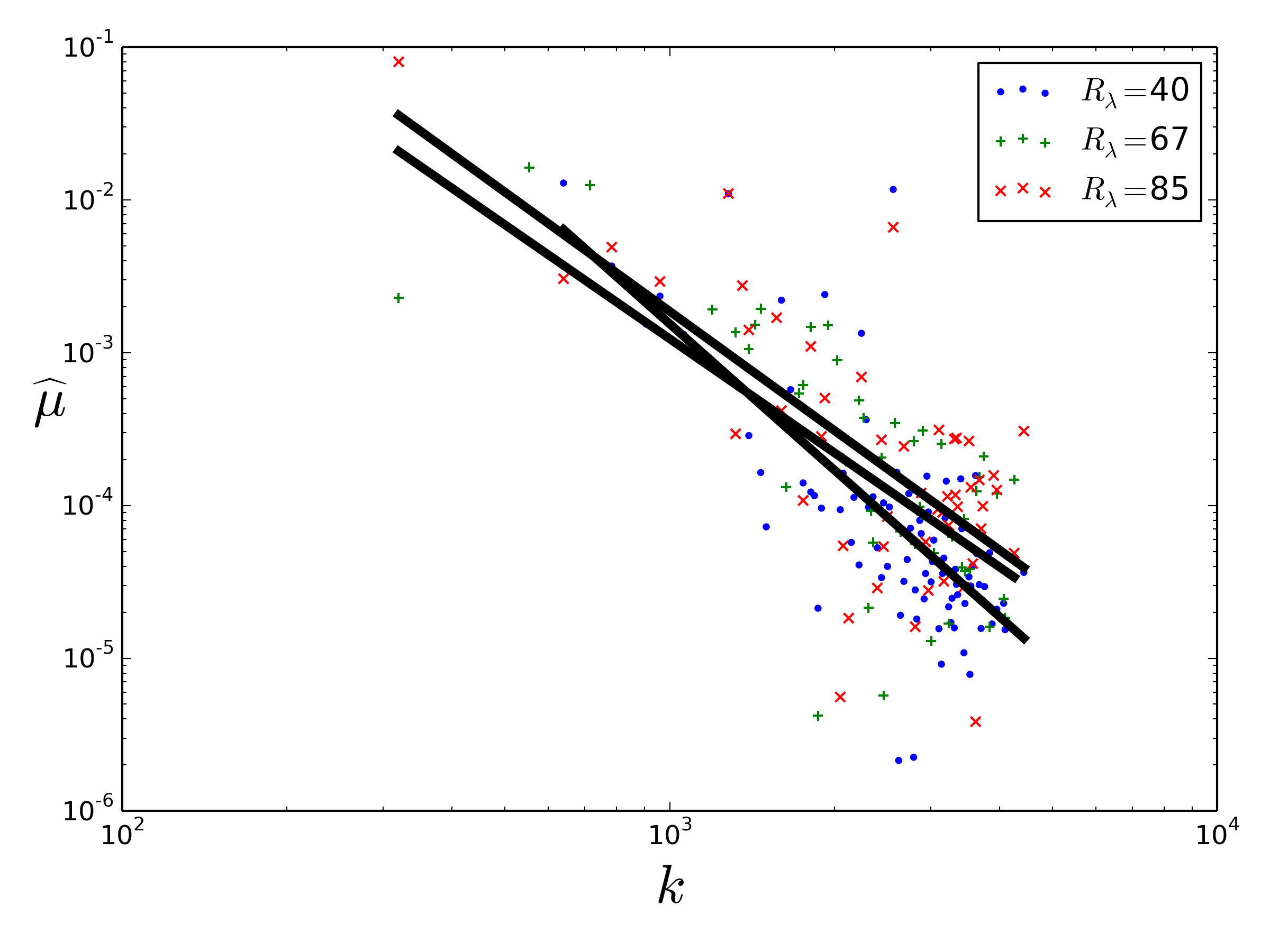
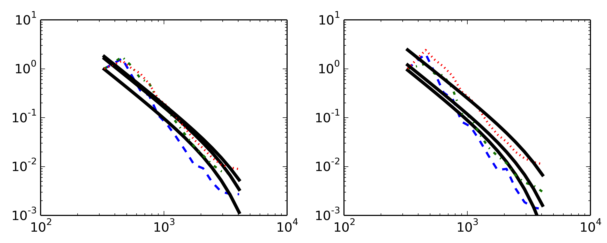
In Fig. 2, we plot vs. in scaled variables. Observe the approximate scaling law , with corrections coming from the dissipation range of scales. Included in the plot is a model curve of the form
| (8) |
The coefficients in this model fit are tabuleted in Table 2.
| 561 | 1577 | 2539 | |
|---|---|---|---|
| 561 | 1577 | 2539 | |
|---|---|---|---|
| 561 | 1577 | 2539 | 561 | 1577 | 2539 | |
III.2 in Fourier space
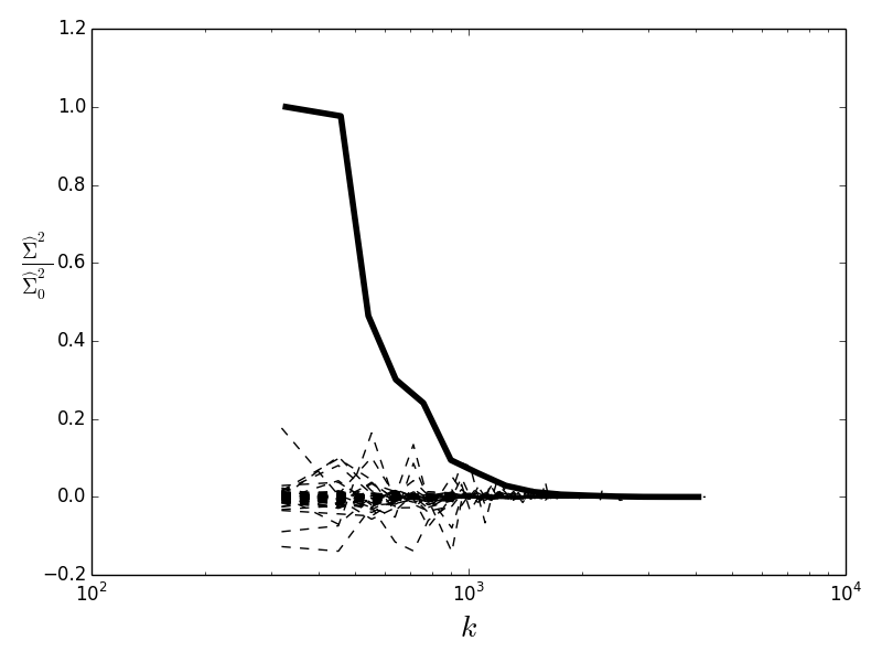
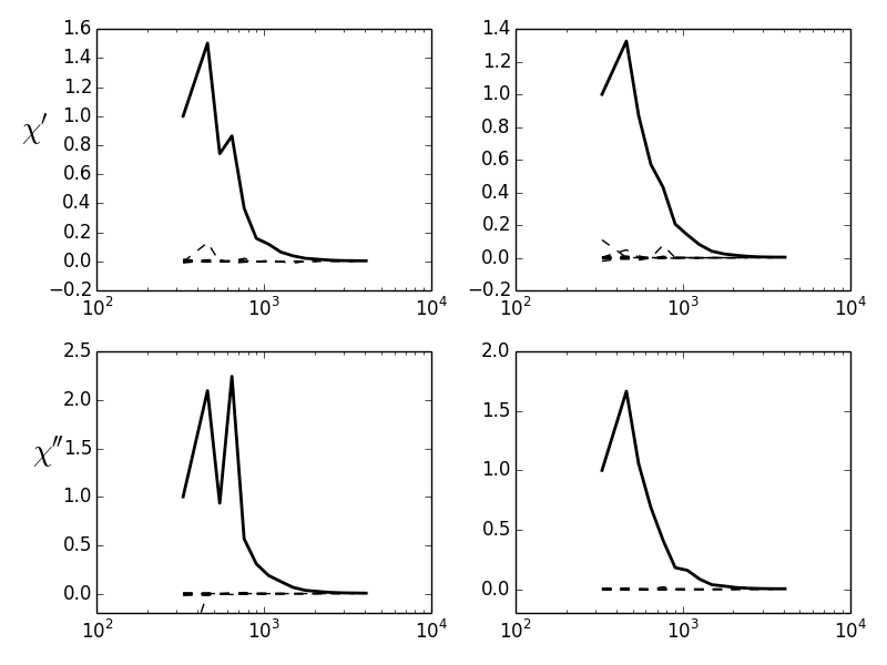
In Fig. 3, we plot the diagonal and off diagonal elements of the covariance matrix for Reynolds number 2549. The smooth curve in the upper part of the figure represent the plot of the diagonal elements as a function of the frequency , while the noisy data near the bottom of the plot are the collection of all off diagonal elements, plotted vs. . The other Reynolds numbers give similar plots. We conclude that the covariance is, within a good approximation, diagonal.
Our modeling for (and for related operators describing the strain matrix and its individual matrix entries in Sec. IV) is based on a simple approximation, which appears to be consistent with the DNS data as examined here. We note that the two random variables contributing to the covariance are orthogonal for and so the terms vanish. In other words, the Fourier coefficient of is , which we write as . In our DNS case, is a matrix before binning.
The Fourier coefficients for for distinct angular variables are statistically independent. For distinct values of the scalar Fourier amplitude , we also assume statistical independence. These assumptions lead to a simple model for , tractable for practical use.
We regard the wave number as an observable on the random field , with the variance for this observation. We derive dependent scaling laws. Approximately, the subspace of the Hilbert space in which is defined has dimension proportional to , namely the area of a sphere in momentum space of radius . Assuming equipartion of the variance of within this subspace, the inverse covariance is a multiple of the identity there. We extend the variance equipartition hypothesis, meaning a uniform level of variance, to distinct values. The subspace variance is then proportional to .
From a more probabilistic point of view, we regard the observation as the result of asking questions, postulated to be independent: what is the variance of associated with each lying on the sphere of radius ? Combining the variance of independent quantities gives the same answer.
Volume scaling laws apply to the volume dependent coefficients in the scaling law for , and use a similar reasoning. Thus, again assuming equipartition, the mesh cell averages over a single coarse grid resoled cell scale with . In summary, we propose scaling laws for in terms of the scalar wave number and spatial volume, with the dispersion relation
| (9) |
with dimensionless constants , to be determined. The factors and are volumes for physical space and Fourier space. The term, not previously discussed, is postulated to capture the leading order viscous corrections to the otherwise purely inertial range theory.
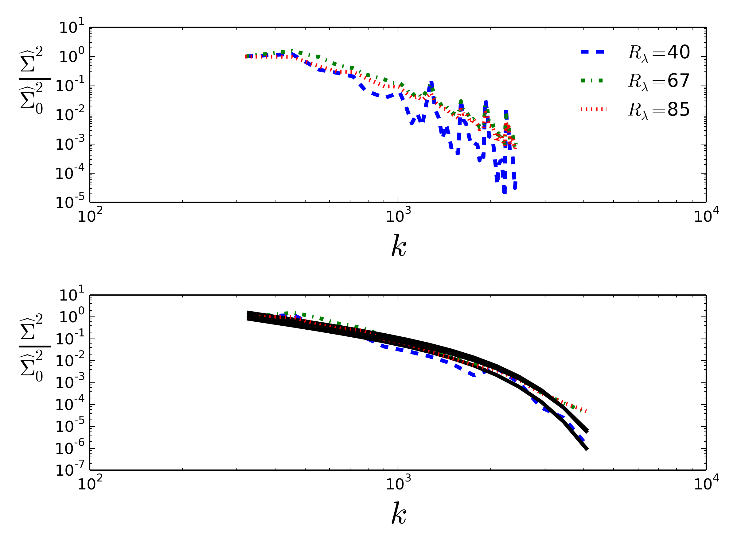
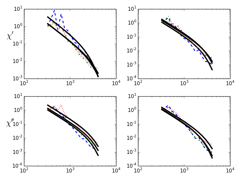
In Fig. 4, we plot vs. on scales with the model curves (9) superimposed, based on optimal choices of the coefficients . We first fit in the inertial range (small values), and then fit over a 1/2 decade at the end of the interial range. We observe that most of the Reynolds number dependence of the has been removed by the scaling introduced here, see Table 2.
IV A log normal model for velocity gradients
We repeat the analysis of Secs. II – III.2 for the strain matrix restricted to subspaces. Let and be self adjoint projection operators on , and consider the reduced strain matrix . In more detail, we consider
| (10) |
and the associated . Thus is the strain associated with fluid velocities in directions spaned by and fluctuations occurring with spatial variation in directions spanned by .
With the rescaled resolved grid level mean for the rescaled , is the rescaled covariance
| (11) | ||||
With these changes, we repeat the analysis of Figs. 1–4 with the modified dispersion relation
| (12) | ||||
and modified coefficients and . We assume that and are both one dimensional.
We also show that the tensor dissipation operators
| (13) |
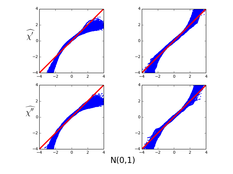
satisfy log normal statistics. Here the exponential and the log in the definition of log normal ( and ) is considered in the sense of matrix operations. See Figs. 7, 8 and 9.
We note that the matrix QQ plots, and to some extent, all the QQ plots, raise the possibility of nonGaussian statistics as a correction to the normal and log normal statistics assumed here. Especially in Fig. 7, systematic corrections to the Gaussian property show smaller positive excursions and stronger negative excursions for than Gaussian for the diagonal matrix elements. Both the negative and positive differential excursions reflect a smaller and a possible bias toward a laminar rather than turbulent flow. In contrast, the off diagonal QQ plots suggest stronger excursions than Gaussian for both positive and negative excursions, a phenomena known as heavy tails in the statistical data analysis literature. These are the matrix elements which occur in vortex stretching and folding, commonly believed to be an important element of fully developed turbulence.
V Discussion
Verification by computational studies will typically encounter only a limited range of LES unresolved scales, compared to a finely gridded simulation. But the previous analysis, when applied over many scales, has a conceptual flaw. If there is no resetting of the parameters within the statistics model of a single resolved scale, then we could apply this theory in the absence of the coarsely gridded LES to the entire computation. Doing this would remove the rescaling already seen to be important. For this reason, we restrict the model to a small range of unresolved scales. In a future publication we reformulate the model in a renormalization group manner in the case of multiple scales.
In an LES context, we analyze the unresolved scales statistically, with an emphasis on the strain rate and its logarithm . Resolved scale adjustments to the mean and variance for lead to a theory for the resulting covariance . We find that is approximately diagonal in Fourier space. An equipartition hypothesis for the variance of leads to a new power scaling law and a simple parameterization for , verified by comparison to DNS over about a decade of LES unresolved inertial scales. For reasons discussed, we restrict this theory to a single or limited range within the inertial range of scales. This pure dissipation rate model is extended to the individual velocity gradient components and to the tensor dissipation rates and .
Open questions, to be addressed in future work, concern temporal statistics of turbulent intensity, statistical models for the velocity gradients and strongly nonhomogeneous flows, such as boundary layers.
References
- [1] G. I. Barenblatt and A. J. Chorin. New perspectives in turbulence: Scaling laws, asymptotics, and intermittency. SIAM Review, 40:265–291, 1998.
- [2] A. Chorin. Vorticity and Turbulence. Springer Verlag, New York–Heidelberg–Berlin, 1994.
- [3] David Jou. Intermittent turbulence: a short introduction. Scientia Marina, 61:57–62, 1997.
- [4] A. N. Kolmogorov. Local structure of turbulence in incompressible viscous fluid for very large Reynolds number. Doklady Akad. Nauk. SSSR, 30:299–3031, 1941.
- [5] A. N. Kolmogorov. A refinement of previous hypotheses concerning the local structure of turbulence in a viscous incompressible fluid at high reynolds number. J. Fluid Mechanics, 13:82–85, 1962.
- [6] A. S. Monin and A. M. Yaglom. Statistical Fluid Mechanics: Mechanics of Turbulence. MIT Press, Cambridge, MA, 1971.
- [7] A. M. Oboukhov. Some specific features of atmospheric tubulence. J. Fluid Mech., 13:77–81, 1962.
- [8] S.B. Pope and Y.L. Chen. The velocity-dissipation probability density function model for turbulent flows. Phys. Fluids A, 2, 1990.
- [9] H. Pouransari, H. Kolla, J.H. Chen, and A. Mani. Spectral analysis of energy transfer in variable density, radiatvely heated particle-laden flows. Proceedings of the Summer Program, Center for Turbulence Research, pages 27–36, 2014.
- [10] K. R. Sreenivasan. Possible effects of small-scale intermittancy in turbulent combustion. Flow, Turbulence and Combustion, 72:115–131, 2004.
- [11] P. K. Yeung and S. B. Pope. Lagrangian statistics from direct numerical simulations of isotropic turbulence. J. Fluid Mech, 207:531–586, 1989.