Relating correlation measures: the importance of the energy gap

Abstract

The concept of correlation is central to all approaches that attempt the description of many-body effects in electronic systems. Multipartite correlation is a quantum information theoretical property that is attributed to quantum states independent of the underlying physics. In quantum chemistry, however, the correlation energy (the energy not seized by the Hartree-Fock ansatz) plays a more prominent role. We show that these two different viewpoints on electron correlation are closely related. The key ingredient turns out to be the energy gap within the symmetry-adapted subspace. We then use a few-site Hubbard model and the stretched H₂ to illustrate this connection and to show how the corresponding measures of correlation compare.

I Introduction

Since P.-O. Löwdin in the fifties, one usually defines correlation energy in quantum chemistry by the difference between the exact ground state (GS) energy of the system and its Hartree-Fock (HF) energy Löwdin (1955):

$$E_{\rm corr}=E_{\rm GS}-E_{\rm HF}.$$ (1)

Since $E_{\rm HF}$ is an upper bound on $E_{\rm GS}$ the correlation energy is negative by definition. Beyond HF theory, numerous other methods (such as, e.g., configuration interaction or coupled-cluster theory) aim at reconstructing the part of the energy missing from a single-determinantal description. In fact, one common indicator of the accuracy of a method is the percentage of the correlation energy it is able to recover. Rigorous estimates of the error of the HF energy are already known for Coulomb systems with large atomic numbers Bach (1992).

In density-functional theory (DFT), nowadays the workhorse theory for both quantum chemistry and solid-state physics, the correlation energy has a slightly different definition. Instead of HF energy, one can use as reference the energy obtained by the (exchange only) optimized effective potential method Sharp and Horton (1953); Talman and Shadwick (1976); Kümmel and Kronik (2008) which is slightly higher than the HF energy. Clearly, the choice of the reference energy is arbitrary, as the correlation energy is not a physical observable. It remains, however, a very useful tool in understanding and quantifying the magnitude of many-body effects in given systems.

In recent years a considerable effort has been devoted to characterize the correlation of a quantum system from a quantum-information theoretical viewpoint Horodecki et al. (2009). A priori, fermionic correlation is a property of the many-electron wave function. For the ground state $|\Psi_{\rm GS}\rangle$, the total correlation can be quantified by the minimal (Hilbert-Schmidt) distance of $|\Psi_{\rm GS}\rangle$$\langle\Psi_{\rm GS}|$ to a single Slater determinant state Shimony (1995); Myers and Wu (2010); D’Amico et al. (2011) or just to the HF ground state $|\Psi_{\rm HF}\rangle$$\langle\Psi_{\rm HF}|$,

$$D(\Psi_{\rm GS},\Psi_{\rm HF}) \equiv \frac{1}{2}{\rm Tr}\Big{[}\big{(}\mbox{$|\Psi_{\rm GS}\rangle$}\!\mbox{$\langle\Psi_{\rm GS}|$}-\mbox{$|\Psi_{\rm HF}\rangle$}\!\mbox{$\langle\Psi_{\rm HF}|$}\big{)}^{2}\Big{]}$$ (2)

$$= 1-\big{|}\langle\Psi_{\rm GS}\mbox{$|\Psi_{\rm HF}\rangle$}\big{|}^{2}.$$

This is closely related to the $L^{2}$-norm $\|\Psi_{\rm GS}-\Psi_{\rm HF}\|^{2}$, that however is not a good distance measure since it depends on the global phases of the respective states (which remains a problem even after restricting to real-valued wave functions). The distance (2) is bounded between 0 and 1, reaching the upper value when the overlap between the two wave functions vanishes. Note that maximising this distance for fixed $|\Psi_{\rm GS}\rangle$ over all single Slater determinants is not equivalent to the minimisation of the energy that leads to the Hartree-Fock orbitals. In fact, such procedure leads to the so-called Brueckner orbitals Löwdin (1962); Zhang and Mauser (2016), which are more “physical” than Hartree-Fock or Kohn-Sham orbitals, as they represent much better single-particle quantities Lindgren, Lindgren, and Mårtensson (1976); Lindgren (1985); Heßelmann and Jansen (2000). We note in passing that in DFT it is less common to measure correlation from the overlap of the wave functions, as the Kohn-Sham Slater determinant describes a fictitious system and not a real one. Further correlation measures involving directly the $N$-fermion wave function are the Slater rank for two-electron systems Schliemann et al. (2001); Plastino, Manzano, and Dehesa (2009), the entanglement classification for the three-fermion case Sárosi and Lévay (2014) or the comparison with uncorrelated states Gottlieb and Mauser (2005).

The nonclassical nature of quantum correlations and entanglement has enormous implications for quantum cryptography or quantum computation. Yet, quantifying correlations and entanglement for systems of identical particles is a part of an ongoing debate Balachandran et al. (2013); Killoran, Cramer, and Plenio (2014); Benatti, Alipour, and Rezakhani (2014); Iemini, Maciel, and Vianna (2015); Miklin, Moroder, and Gühne (2016). From a practical viewpoint, measuring correlation is even more challenging for identical particles since typically only one- and possibly two-particle properties are experimentally accessible. As a consequence, also simplified correlation measures involving reduced density operators were developed. These are, e.g., the squared Frobenius norm of the cumulant part of the two-particle reduced density matrix Juhász and Mazziotti (2006), the entanglement spectrum and its gap Li and Haldane (2008); Thomale et al. (2010), the von-Neumann entropy $S(\hat{\rho}_{1})=-\mbox{Tr}[\hat{\rho}_{1}\log{\hat{\rho}_{1}}]$ of the one-particle reduced density operator $\hat{\rho}_{1}$ or just the $l^{1}-$distance $\delta(\vec{n})$ of the decreasingly-ordered natural occupation numbers $\vec{n}$ (the eigenvalues of $\hat{\rho}_{1}$) to the “Hartree-Fock”-point $\vec{n}_{\rm HF}=(1_{1},\ldots,1_{N},0_{N+1},\ldots)$ Schilling, Gross, and Christandl (2013).

A first elementary relation between all those correlation measures and the concept of correlation energy is obvious: Each measure attains the minimal value zero whenever the exact ground state is given by a single Slater determinant Helbig, Tokatly, and Rubio (2010), i.e. the correlation energy vanishes. Furthermore, a monotonous relationship between the von-Neumann entropy of $\hat{\rho}_{1}$ and the density functional definition of correlation energy has already been observed for some specific systems Smith, Schmider, and Smith (2002); Benavides-Riveros, Gracia-Bondía, and Várilly (2012); Benavides-Riveros, Toranzo, and Dehesa (2014).

In this paper we establish a connection between those two viewpoints on electron correlation by providing a concise universal relation between the distance measure (2) and the correlation energy $E_{\rm corr}$. Furthermore, due to the continuity of the partial trace similar relations between measures involving reduced density operators and $E_{\rm corr}$ follow then immediately.

The paper is arranged as follows. Section II presents our main results, while section III illustrates them for molecular systems. The last section provides a conclusion. Technical aspects of our work are presented in the appendix.

II Main results

Our starting point is the following theorem. Let $\hat{H}$ be a Hamiltonian on the Hilbert space $\mathcal{H}$ with a unique ground state $|\Psi_{\rm GS}\rangle$ and an energy gap $E_{\rm gap}=E_{\rm ES}-E_{\rm GS}$ to the first excited state. Then, for any $\mbox{$|\Psi\rangle$}\in\mathcal{H}$ with energy $E=\mbox{$\langle\Psi|$}\hat{H}\mbox{$|\Psi\rangle$}$ we have

$$|\mbox{$\langle\Psi_{\rm GS}|$}\Psi\rangle|^{2}\geq\frac{E_{\rm ES}-E}{E_{\rm gap}}.$$ (3)

The significance of this theorem concerns the case of energy expectation values $E=\mbox{$\langle\Psi|$}\hat{H}\mbox{$|\Psi\rangle$}$ within the energy gap $[E_{\rm GS},E_{\rm ES}]$, and relates the energy picture with the structure of the quantum state. A state $|\Psi\rangle$ has a good overlap with the ground state whenever its energy expectation value $E$ is close to the ground state energy, when measured relatively to the energy gap $E_{\rm gap}$.

To prove this theorem we use the spectral decomposition of $\hat{H}=\sum_{E}E\hat{P}_{E}$, where $\hat{P}_{E}$ is the orthogonal projection operator onto the eigenspace of energy $E$. This yields

$$E=\mbox{$\langle\Psi|$}\hat{H}\mbox{$|\Psi\rangle$} \geq E_{\rm GS}\mbox{$\langle\Psi|$}\hat{P}_{\rm GS}\mbox{$|\Psi\rangle$}+E_{\rm ES}\sum_{E\geq E_{\rm ES}}\mbox{$\langle\Psi|$}\hat{P}_{E}\mbox{$|\Psi\rangle$}$$

$$=E_{\rm GS}\mbox{$\langle\Psi|$}\hat{P}_{\rm GS}\mbox{$|\Psi\rangle$}+E_{\rm ES}(1-\mbox{$\langle\Psi|$}\hat{P}_{\rm GS}\mbox{$|\Psi\rangle$}),$$

where we used in the last line $\sum_{E\geq E_{\rm ES}}\hat{P}_{E}=\mathbb{1}-\hat{P}_{\rm GS}$. By using $\mbox{$\langle\Psi|$}\hat{P}_{\rm GS}\mbox{$|\Psi\rangle$}=|\mbox{$\langle\Psi_{\rm GS}|$}\Psi\rangle|^{2}$ this leads to Eq. (3) which completes the proof.

From this result, we can deduce that the distance between the ground state of any Hamiltonian (with a unique ground state) and the corresponding HF ground state is bounded from above by a function depending on the energy gap of the system according to

$$D(\Psi_{\rm GS},\Psi_{\rm HF})\leq\frac{|E_{\rm corr}|}{E_{\rm gap}}.$$ (4)

In practice, the Hamiltonian at hand typically exhibits symmetries. For instance, the electronic Hamiltonian $\hat{H}$ of atoms and molecules commutes with the total spin. The ground state inherits this symmetry, i.e. it lies in an eigenspace $\mathcal{H}_{\sigma}=\hat{\pi}_{\sigma}\mathcal{H}$ of the symmetry operators, where $\hat{\pi}_{\sigma}$ denotes the restriction to that subspace with eigenvalue $\sigma$. Numerical methods are usually adapted to the ground state symmetry (if possible). A prime example is the restricted HF, a specific HF ansatz for approximating ground states with the correct spin symmetries. These considerations on symmetries allow for a significant improvement of estimate (4): $|\Psi_{\rm GS}\rangle$ and $|\Psi_{\rm HF}\rangle$ are not only ground state and HF ground state of $\hat{H}$, respectively, but also of the restricted Hamiltonian

$$\hat{H}_{\sigma}=\hat{\pi}_{\sigma}\hat{H}\hat{\pi}_{\sigma}^{\dagger}$$ (5)

acting on the symmetry-adapted Hilbert space $\mathcal{H}_{\sigma}$. Application of the estimate (4) to $\hat{H}_{\sigma}$ implies an improved upper bound: $E_{\rm gap}$ no longer refers to the gap to the first excited state but to the first excited state within the symmetry-adapted space $\mathcal{H}_{\sigma}$ of the ground state (and may therefore increase considerably). In the following, $E_{\rm ES}$ will therefore stand for the energy of the first excited state with the same symmetries as the ground state.

The estimate (4) is our most significant result. It establishes a connection between both viewpoints on electron correlation and shows that the dimensionless quantity $|E_{\rm corr}|/E_{\text{gap}}$ provides a universal upper bound on correlations described by the wave function. This result also underlines the importance of the energy gap being the natural reference energy scale. Furthermore, it is worth noting that estimate (4) implies a similar estimate for the simplified correlation measure $\delta(\vec{n})=\mbox{dist}_{l^{1}}(\vec{n},\vec{n}_{\rm HF})=\sum_{i=1}^{N}(1-n_{i})+\sum_{j>N}n_{j}$, since (see Appendix A):

$$\frac{\delta(\vec{n})}{2N}\leq D(\Psi_{\rm GS},\Psi_{\rm HF}).$$ (6)

Before we continue a note of caution is in order here. One might be tempted to apply estimate (4) to metals. However, since metals have a vanishing energy gap and also $E_{\rm ES}=E_{\rm GS}<E_{\text{HF}}$, i.e. $|E_{\rm corr}|>E_{\rm gap}$, our estimate has no relevance for them.

To illustrate our results, in the next section we use simple, analytically solvable systems, namely the two- and three-site Hubbard model, which are well known for their capability of exhibiting both, weak and strong (static) correlation. We study also the stretching of H₂, which is considered a paradigm of the difficulties that single-determinant methods have with bond dissociation Fuchs et al. (2005).

III Numerical investigations

III.1 Hubbard model

Besides its importance for solid-state physics, the Hubbard model is one of the paradigmatic instances used to simplify the description of strongly correlated quantum many-body systems. The Hamiltonian (in second quantization) of the one-dimensional $r$-site Hubbard model reads:

$$\hat{H}=-\frac{t}{2}\sum_{i,\sigma}(c^{\dagger}_{i\sigma}c_{(i+1)\sigma}+h.c.)+2U\sum_{i}\hat{n}_{i\uparrow}\hat{n}_{i\downarrow},$$ (7)

$i\in\{1,2,\dots,r\}$, where $c^{\dagger}_{i\sigma}$ and $c_{i\sigma}$ are the fermionic creation and annihilation operators for a particle on the site $i$ with spin $\sigma\in\{\uparrow,\downarrow\}$ and $\hat{n}_{i\sigma}=c^{\dagger}_{i\sigma}c_{i\sigma}$ is the particle-number operator. The first term in Eq. (7) describes the hopping between two neighboring sites while the second represents the on-site interaction. Periodic boundary conditions in the case $r>2$ are also assumed. Achieved experimentally very recently with full control over the quantum state Murmann et al. (2015), this model may be considered as a simplified tight-binding description of the H_r molecule Olsen and Thygesen (2014).

For two fermions on two sites, the eigenstates of $\hat{H}$ are described by four quantum numbers $|E,s,m,p\rangle$, $E$ being the energy, $(s,m)$ the spin eigenvalues and $p$ the eigenvalue of the operator swapping both sites. The dimension of the Hilbert space is $6$, which splits in two parts according to the total spin: There are three triplet spin states with 0-energy, $|0,1,1,-1\rangle$, $|0,1,-1,-1\rangle$ and $|0,1,0,-1\rangle$, and three singlets, one of them $|2U,0,0,-1\rangle$. The other two singlets $|E_{\rm GS},0,0,1\rangle$ and $|E_{\rm ES},0,0,1\rangle$ span the spin and translation symmetry-adapted Hilbert space $\mathcal{H}_{0,0,1}$. A straightforward computation yields for the ground state $E_{\rm GS}=U-\sqrt{U^{2}+t^{2}}$ and for the excited state $E_{\rm ES}=U+\sqrt{U^{2}+t^{2}}$. The restricted HF energy, $E_{\rm HF}=-t+U$, is a reasonable approximation to the exact ground state energy only for small values of $U/t$. The unphysical behaviour observed for larger values can be explained by the contribution of ionic states to the HF wave function Ziesche et al. (1997). The energy gap is given by $2\sqrt{U^{2}+t^{2}}$. Since the subspace of $s=m=0$ and $p=+1$ is two-dimensional and since the restricted HF ground state belongs to it as well, we have that the equality in (4) holds: $D(\Psi_{\rm GS},\Psi_{\rm HF})=|E_{\rm corr}|/E_{\rm gap}$.

For the ground state $|\Psi_{\rm GS}\rangle$, the corresponding natural occupation numbers follow as $n_{\pm}(U/t)=(1\pm 1/\sqrt{1+U^{2}/t^{2}})/2$, each one with multiplicity two. Note that by defining the dimensionless energy gap $\Delta=E_{\rm gap}/t$ we can express the occupation numbers as a function of $\Delta$, leading to $n_{\pm}(\Delta)=1/2\pm 1/\Delta$. This result shows that the one-particle correlation measures (von-Neumann entropy and $\delta$-distance) also depend on the energy gap. In particular, the distance of the natural occupation numbers to the HF-point follows as $\delta(\Delta)=2-4/\Delta$ which turns out to saturate the inequality (6).

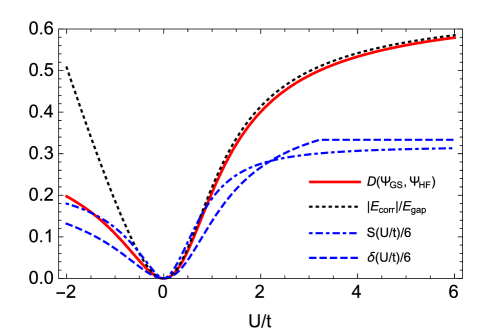
Figure 1: For the Hubbard model for three fermions on three sites we present several correlation measures as functions of the dimensionless coupling $U/t$. These are the distance $D(\Psi_{\rm HF},\Psi_{\rm GS})$ of the GS to the HF state, $|E_{\rm corr}|/E_{\rm gap}$ and the one-particle correlation measures $S$, $\delta$ (see text).

To study the Hubbard model for more than two sites, we first recall that the Hamiltonian (7) commutes with the total spin vector operator, its $z$-component and the translation operator (from the lattice site $i$ to the next site $i+1$), with eigenvalues $e^{i2\pi p/r}$ with $p\in\{0,1,\dots,r-1\}$. The Hamiltonian is block diagonal with respect to those symmetries (see Appendix B). For the case of three fermions on three sites, the spectrum of the Hubbard model restricted to the subspace that corresponds to $s=\scriptstyle\frac{1}{2}$, $m=\scriptstyle\frac{1}{2}$ and $p=2$ is given by Schilling (2015):

$$E_{j}(U,t)=-2\sqrt{Q}\cos\bigg{(}\frac{\theta-2\pi j}{3}\bigg{)}+\frac{4U}{3},\quad j\in\{0,1,2\},$$

where $Q=28U^{2}/9+3t^{2}/4$ and $\cos\theta=8U^{3}/(27Q^{3/2})$. The dimensionless energy gap is $\Delta(U/t)=(E_{\rm ES}-E_{\rm GS})/t=-2\sqrt{3Q}\sin[(\theta-\pi)/3]/t$. For positive values of the dimensionless coupling $U/t$, $\Delta(U/t)=3/2+4(U/t)^{2}/9+\mathcal{O}((U/t)^{3})$. For negative values, the energy gap is bounded from above: $\Delta(U/t)\rightarrow 1.73205$.

In Fig. 1 we plot several correlation measures as a function of $U/t$ for this model. As expected, all curves increase monotonically with the strength of the interaction. For the positive region $U/t\geq 0$, the curve for $|E_{\rm corr}|/E_{\rm gap}$ follows very closely the one for $D(\Psi_{\rm GS},\Psi_{\rm HF})$ confirming the significance of our estimate (4). Both curves converge to the same value ($2/3$) for $U/t\rightarrow\infty$ . However, for negative values of $U/t$ the estimate loses its significance. This is based on the fact that a significant part of the weight of the HF ground state lies on higher excited states. In addition, the energy gap is getting of the same order of magnitude as the correlation energy, leading to a rapid growth of our bound. In the strong correlation regime, beyond $U/t<-3.375$, $|E_{\rm corr}|>E_{\rm gap}$ and our estimate has no significance. For positive values of $U/t$ the energy gap increases monotonously. Note that the quantity $|E_{\rm corr}|/E_{\rm gap}$ provides a much better estimate on the quantum state overlap (2) than the von-Neumann entropy or the $l^{1}-$distance to the HF-point. The latter ones (the blue curves in Fig. 1) saturate very soon in contrast to the red and black ones. This shows the limitation of the one-particle picture to measure total fermion correlation.

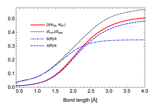
Figure 2: For the stretched H₂ we present several correlation measures as functions of the bond length. These are the distance $D(\Psi_{\rm HF},\Psi_{\rm GS})$ of the GS to the HF state, $|E_{\rm corr}|/E_{\rm gap}$ and the one-particle correlation measures $S$, $\delta$ (see text).

III.2 The stretched H₂

As a second example we look at the archetypal instance of strong (static) correlation, i.e. the stretched dihydrogen H₂ Coulson and Fischer (1949), which we analyze numerically using a cc-pVTZ basis set. In its dissociation limit, this system is commonly used as a benchmark to produce exchange-correlation functionals for strong static correlations Baerends (2001); Matito et al. (2016). The HF approach describes well the equilibrium chemical bond, but fails dramatically as the molecule is stretched. It is also known that DFT functionals describe the covalent bond well, but the predicted energy is overestimated in the dissociation limit due to delocalization, static-correlation and self-interaction errors Cohen, Mori-Sánchez, and Yang (2008). Around the equilibrium separation (0.74 Å), electronic correlation is not particularly large and the HF state therefore approximates significantly well the ground-state wave function. The first excited state of H₂ with the same symmetry of the ground state ($s=m=0$) is the second excited state. Around the equilibrium geometry, the energy gap diminishes as the interatomic distance is elongated. As for the two-site Hubbard model, close to equilibrium, the bound $|E_{\rm corr}|/E_{\rm gap}$ provides a good estimate on the correlation measure $D(\Psi_{\rm GS},\Psi_{\rm HF})$. Remarkably, as shown in Fig. 2, beyond the equilibrium bound, where the static correlation effects can be observed, $|E_{\rm corr}|/E_{\rm gap}$ reproduces the behaviour of the distance $D(\Psi_{\rm GS},\Psi_{\rm HF})$. The same holds for the $\delta$-distance, which is largely due to the fact that for two-fermion models the value of the first occupation number is approximately the square of the projection of the ground state onto the HF configuration. In contrast, the von-Neumann entropy saturates very soon.

IV Conclusion

In conclusion, we have connected both viewpoints on fermion correlation by providing the universal estimate (4). It connects the measure of total fermion correlation (as property that can be attributed to quantum states independent of the underlying physics) and the correlation energy (commonly used in quantum chemistry). The quantity that connects both measures is the energy gap of the corresponding block Hamiltonian with the same symmetry as the ground state. Moreover, due to the continuity of the partial trace, similar estimates follow for several correlation measures resorting to reduced-particle information only. Yet, as it can be inferred from their early saturation shown in Fig. 1, the significance of such simplified correlation measures is limited.

Since the quantity $|E_{\rm corr}|/E_{\rm gap}$ provides an estimate on the overlap between the HF and the exact ground state wave function our work may allow one to use the sophisticated concept of multipartite entanglement developed and explored in quantum information theory for a more systematic study of strongly correlated systems. In particular, our work suggests an additional tool for describing the possible failure of DFT in reconstructing specific properties of a given quantum system. This failure can be either attributed to a rather poor reconstruction of the systems ground state energy or to the failure of the effective method (e.g. Kohn-Sham) in reconstructing many-particle properties from one-particle information. The latter case would be reflected by poor saturation of the inequality (4) while the first one corresponds to a large correlation energy (requiring a multi-reference method instead Cohen, Mori-Sánchez, and Yang (2008); Hellgren et al. (2015); Benavides-Riveros and Schilling (2016); Schilling, Benavides-Riveros, and Vrana (2017)).

Appendix A Proof of estimate (6)

We consider an $N$-fermion Hilbert space $\mathcal{H}_{N}^{(f)}$ where the underlying one-particle Hilbert space $\mathcal{H}_{1}^{(d)}$ has dimension $d\in\mathbb{N}\cup\{\infty\}$. For $\mbox{$|\Psi\rangle$}\in\mathcal{H}_{N}^{(f)}$ we can determine its one-particle reduced density operator $\hat{\rho}_{1}$ (trace-normalized to $N$) and the vector $\vec{\lambda}=(\lambda_{i})_{i=1}^{d}$ of decreasingly-ordered eigenvalues of $\hat{\rho}_{1}$ (natural occupation numbers). Let $\{\mbox{$|\chi_{j}\rangle$}\}_{j=1}^{d}$ be a Brueckner orthonormal basis for $\mathcal{H}_{1}^{(d)}$, i.e. the specific Slater determinant $\mbox{$|\bm{\chi}\rangle$}=\mbox{$|\chi_{1},\ldots,\chi_{N}\rangle$}$ maximizes the overlap with $|\Psi\rangle$. Furthermore we introduce $\delta(\vec{x})=\sum_{i=1}^{N}(1-x_{i})+\sum_{j=N+1}^{d}x_{j}$ and $\hat{n}_{i}$ as the particle number operator for state $|\chi_{i}\rangle$. Obviously, $\delta(\vec{\lambda})$ is the $l^{1}$-distance of $\vec{\lambda}$ to the “Hartree-Fock”-point $(1,\ldots,1,0,\ldots)$. In the following we prove the estimate

$$\frac{\delta(\vec{\lambda})}{2\,\mbox{min}(N,d-N)}\leq 1-|\langle\bm{\chi}\mbox{$|\Psi\rangle$}|^{2}\,.$$ (8)

For this, we introduce the particle number expectation values $n_{i}=\mbox{$\langle\Psi|$}\hat{n}_{i}\mbox{$|\Psi\rangle$}$ and $\hat{\delta}=\delta((\hat{n}_{i})_{i=1}^{d})$. Since the spectrum of $\hat{\delta}$ is given by $\{0,1,\ldots,2M\}$ with $M=\mbox{min}(N,d-N)$ we find

$$\delta(\vec{n}) =\mbox{$\langle\Psi|$}\hat{\delta}\mbox{$|\Psi\rangle$}=\sum_{d=1}^{2M}d\,\|\hat{P}_{d}\Psi\|_{L^{2}}^{2}\leq 2M\sum_{d=1}^{2M}\|\hat{P}_{d}\Psi\|_{L^{2}}^{2}$$

$$=2M\,\big{(}1-\|\hat{P}_{0}\Psi\|_{L^{2}}^{2}\big{)}\,,$$ (9)

where we have used the spectral decomposition $\hat{\delta}=\oplus_{d=0}^{2M}\,d\,\hat{P}_{d}$ of $\hat{\delta}$. By using $\hat{P}_{0}=\mbox{$|\bm{\chi}\rangle$}\!\mbox{$\langle\bm{\chi}|$}$ and the fact that the vector $\vec{\lambda}$ of decreasingly-ordered eigenvalues of $\hat{\rho}_{1}$ majorizes any other vector of occupation numbers (particularly $\vec{n}$) we obtain

$$\delta(\vec{\lambda})\leq\delta(\vec{n})\leq 2M\big{(}1-|\langle\bm{\chi}\mbox{$|\Psi\rangle$}|^{2}\big{)}\,.$$ (10)

Since $|\bm{\chi}\rangle$ maximizes the overlap with $|\Psi\rangle$, we eventually find for the Hartree-Fock ground state $|\Psi_{\rm HF}\rangle$ (or any other single Slater determinant)

$$\frac{\delta(\vec{\lambda})}{2M}\leq 1-|\langle\Psi_{\rm HF}\mbox{$|\Psi\rangle$}|^{2}\,,$$ (11)

i.e. estimate (6).

Appendix B Analytic solution of the Hubbard model for three electrons on three sites

In this section we recall the analytical solution of the three-site Hubbard model for three electrons which was already presented in Ref. Schilling (2015). For the Hubbard model, the one-body reduced density matrix is diagonal in the basis of the Bloch orbitals, which satisfy $\hat{T}_{1}\mbox{$|q\rangle$}=e^{i\varphi q}\mbox{$|q\rangle$}$, where $\varphi=2\pi/r$, $\hat{T}_{1}$ is the 1-particle translation operator and $\hat{T}=\bigotimes^{N}_{i=1}\hat{T}_{1}$. The creation operators in the Bloch basis set read: $\tilde{c}^{\dagger}_{q\sigma}=\frac{1}{\sqrt{r}}\sum_{k=1}^{r}e^{i\varphi qk}c^{\dagger}_{k\sigma}$, $q\in\{0,1,\dots,r-1\}$. To block diagonalize this Hamiltonian one can employ the natural-orbital basis set generated by $\{\mbox{$|q\rangle$}\}$ and then split the total Hilbert space with respect to the spin quantum numbers $s$ and $m$. For example, the only state with maximal magnetic number $m=r/2$ is $\tilde{c}^{\dagger}_{0\uparrow}\tilde{c}^{\dagger}_{1\uparrow}\cdots\tilde{c}^{\dagger}_{r-1\uparrow}\mbox{$|\rm vac\rangle$}$, which spans the one-dimensional subspace $\mathcal{H}_{\scriptstyle\frac{r}{2},\scriptstyle\frac{r}{2},\eta}$ ($\eta=0$ for $r$ odd or $\eta=r/2$ otherwise), as defined by the direct sum of the total Hilbert space:

$$\mathcal{H}=\bigoplus^{N/2}_{s=s_{-}}\bigoplus^{s}_{m=-s}\bigoplus^{r-1}_{p=0}\mathcal{H}_{s,m,p}.$$ (12)

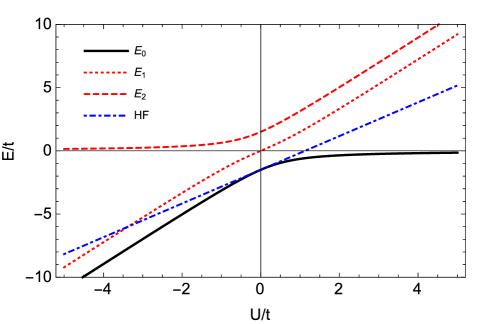
Figure 3: Energy spectrum of the three-site three-fermion Hubbard model restricted to the Hilbert subspace where the ground state lies. The Hartree-Fock energy is also shown.

For the case of three fermions on three sites, the total spin quantum number $s$ can take only two values $\tfrac{3}{2}$ and $\tfrac{1}{2}$. For $s=\tfrac{1}{2}$, thanks to the fact that the Hamiltonian is invariant under simultaneous flipping of all spins, the results for $m=-\tfrac{1}{2}$ are identical to the case $m=\tfrac{1}{2}$. The latter is related to the eight dimensional Hilbert space $\mathcal{H}_{\scriptstyle\frac{1}{2},\scriptstyle\frac{1}{2},2}\oplus\mathcal{H}_{\scriptstyle\frac{1}{2},\scriptstyle\frac{1}{2},1}\oplus\mathcal{H}_{\scriptstyle\frac{1}{2},\scriptstyle\frac{1}{2},0}$, where

$$\mathcal{H}_{\scriptstyle\frac{1}{2},\scriptstyle\frac{1}{2},2}={\rm span}\{\mbox{$|0\uparrow 0\downarrow 2\uparrow\rangle$},\mbox{$|2\uparrow 2\downarrow 1\uparrow\rangle$},\mbox{$|1\uparrow 1\downarrow 0\uparrow\rangle$}\},$$

$$\mathcal{H}_{\scriptstyle\frac{1}{2},\scriptstyle\frac{1}{2},1}={\rm span}\{\mbox{$|0\uparrow 0\downarrow 1\uparrow\rangle$},\mbox{$|2\uparrow 2\downarrow 0\uparrow\rangle$},\mbox{$|1\uparrow 1\downarrow 2\uparrow\rangle$}\}.$$

The translation invariant subspace $\mathcal{H}_{\scriptstyle\frac{1}{2},\scriptstyle\frac{1}{2},0}$ is two dimensional and can be built with two spin-compensated linear combinations of the following three configurations: $|0\uparrow 1\uparrow 2\downarrow\rangle$, $|0\uparrow 1\downarrow 2\uparrow\rangle$ and $|0\downarrow 1\uparrow 2\uparrow\rangle$. As an elementary exercise one verifies that the Hamiltonian restricted to each one of the subspaces $\mathcal{H}_{\scriptstyle\frac{1}{2},\scriptstyle\frac{1}{2},2}$ and $\mathcal{H}_{\scriptstyle\frac{1}{2},\scriptstyle\frac{1}{2},1}$ leads to the same $3\times 3$ matrix. Indeed,

$$\hat{H}|_{\mathcal{H}_{\scriptstyle\frac{1}{2},\scriptstyle\frac{1}{2},1}}=\hat{H}|_{\mathcal{H}_{\scriptstyle\frac{1}{2},\scriptstyle\frac{1}{2},2}}.$$ (13)

It is worth noting that the same configuration appears in the description of the spin-compensated Lithium isoelectronic series Benavides-Riveros, Gracia-Bondia, and Springborg (2013). Moreover, since the diagonalization of any of the Hamiltonians (13) can be performed analytically, an expression for the energy spectrum can be exactly known Schilling (2015):

$$E_{j}=-2\sqrt{Q}\cos\bigg{(}\frac{\theta-2\pi j}{3}\bigg{)}+\frac{4U}{3},$$

for $j=0,1,2$. Here $Q=28U^{2}/9+3t^{2}/4$ and $\cos\theta=8U^{3}/(27Q^{3/2})$. See Fig. 3. The energy gap $E_{\rm gap}$ is then given by $E_{1}-E_{0}$.

References

- Löwdin (1955) P.-O. Löwdin, Phys. Rev. 97, 1509 (1955).
- Bach (1992) V. Bach, Commun. Math. Phys. 147, 527 (1992).
- Sharp and Horton (1953) R. T. Sharp and G. K. Horton, Phys. Rev. 90, 317 (1953).
- Talman and Shadwick (1976) J. D. Talman and W. F. Shadwick, Phys. Rev. A 14, 36 (1976).
- Kümmel and Kronik (2008) S. Kümmel and L. Kronik, Rev. Mod. Phys. 80, 3 (2008).
- Horodecki et al. (2009) R. Horodecki, P. Horodecki, M. Horodecki, and K. Horodecki, Rev. Mod. Phys. 81, 865 (2009).
- Shimony (1995) A. Shimony, Ann. N. Y. Acad. Sci. 755, 675 (1995).
- Myers and Wu (2010) J. M. Myers and T. T. Wu, Quantum Inf. Process. 9, 239 (2010).
- D’Amico et al. (2011) I. D’Amico, J. P. Coe, V. V. França, and K. Capelle, Phys. Rev. Lett. 106, 050401 (2011).
- Löwdin (1962) P. Löwdin, J. Math. Phys. 3, 1171 (1962).
- Zhang and Mauser (2016) J. M. Zhang and N. J. Mauser, Phys. Rev. A 94, 032513 (2016).
- Lindgren, Lindgren, and Mårtensson (1976) I. Lindgren, J. Lindgren, and A.-M. Mårtensson, Z. Phys. A 279, 113 (1976).
- Lindgren (1985) I. Lindgren, Phys. Rev. A 31, 1273 (1985).
- Heßelmann and Jansen (2000) A. Heßelmann and G. Jansen, J. Chem. Phys. 112, 6949 (2000).
- Schliemann et al. (2001) J. Schliemann, J. I. Cirac, M. Kuś, M. Lewenstein, and D. Loss, Phys. Rev. A 64, 022303 (2001).
- Plastino, Manzano, and Dehesa (2009) A. R. Plastino, D. Manzano, and J. S. Dehesa, EPL 86, 20005 (2009).
- Sárosi and Lévay (2014) G. Sárosi and P. Lévay, Phys. Rev. A 89, 042310 (2014).
- Gottlieb and Mauser (2005) A. D. Gottlieb and N. J. Mauser, Phys. Rev. Lett. 95, 123003 (2005).
- Balachandran et al. (2013) A. P. Balachandran, T. R. Govindarajan, A. R. de Queiroz, and A. F. Reyes-Lega, Phys. Rev. Lett. 110, 080503 (2013).
- Killoran, Cramer, and Plenio (2014) N. Killoran, M. Cramer, and M. B. Plenio, Phys. Rev. Lett. 112, 150501 (2014).
- Benatti, Alipour, and Rezakhani (2014) F. Benatti, S. Alipour, and A. T. Rezakhani, New J. Phys. 16, 015023 (2014).
- Iemini, Maciel, and Vianna (2015) F. Iemini, T. O. Maciel, and R. O. Vianna, Phys. Rev. B 92, 075423 (2015).
- Miklin, Moroder, and Gühne (2016) N. Miklin, T. Moroder, and O. Gühne, Phys. Rev. A 93, 020104 (2016).
- Juhász and Mazziotti (2006) T. Juhász and D. A. Mazziotti, J. Chem. Phys. 125, 174105 (2006).
- Li and Haldane (2008) H. Li and F. D. M. Haldane, Phys. Rev. Lett. 101, 010504 (2008).
- Thomale et al. (2010) R. Thomale, A. Sterdyniak, N. Regnault, and B. A. Bernevig, Phys. Rev. Lett. 104, 180502 (2010).
- Schilling, Gross, and Christandl (2013) C. Schilling, D. Gross, and M. Christandl, Phys. Rev. Lett. 110, 040404 (2013).
- Helbig, Tokatly, and Rubio (2010) N. Helbig, I. V. Tokatly, and A. Rubio, Phys. Rev. A 81, 022504 (2010).
- Smith, Schmider, and Smith (2002) G. T. Smith, H. L. Schmider, and V. H. Smith, Phys. Rev. A 65, 032508 (2002).
- Benavides-Riveros, Gracia-Bondía, and Várilly (2012) C. L. Benavides-Riveros, J. M. Gracia-Bondía, and J. C. Várilly, Phys. Rev. A 86, 022525 (2012).
- Benavides-Riveros, Toranzo, and Dehesa (2014) C. L. Benavides-Riveros, I. V. Toranzo, and J. S. Dehesa, J. Phys. B: At. Mol. Opt. Phys. 47, 195503 (2014).
- Fuchs et al. (2005) M. Fuchs, Y.-M. Niquet, X. Gonze, and K. Burke, J. Chem. Phys. 122, 094116 (2005).
- Murmann et al. (2015) S. Murmann, A. Bergschneider, V. M. Klinkhamer, G. Zürn, T. Lompe, and S. Jochim, Phys. Rev. Lett. 114, 080402 (2015).
- Olsen and Thygesen (2014) T. Olsen and K. S. Thygesen, J. Chem. Phys. 140, 164116 (2014).
- Ziesche et al. (1997) P. Ziesche, O. Gunnarsson, W. John, and H. Beck, Phys. Rev. B 55, 10270 (1997).
- Schilling (2015) C. Schilling, Phys. Rev. B 92, 155149 (2015).
- Coulson and Fischer (1949) C. A. Coulson and I. Fischer, Philos. Mag. 40, 386 (1949).
- Baerends (2001) E. J. Baerends, Phys. Rev. Lett. 87, 133004 (2001).
- Matito et al. (2016) E. Matito, D. Casanova, X. Lopez, and J. M. Ugalde, Theor. Chem. Acc. 135, 226 (2016).
- Cohen, Mori-Sánchez, and Yang (2008) A. J. Cohen, P. Mori-Sánchez, and W. Yang, Science 321, 792 (2008).
- Hellgren et al. (2015) M. Hellgren, F. Caruso, D. R. Rohr, X. Ren, A. Rubio, M. Scheffler, and P. Rinke, Phys. Rev. B 91, 165110 (2015).
- Benavides-Riveros and Schilling (2016) C. L. Benavides-Riveros and C. Schilling, Z. Phys. Chem. 230, 703 (2016).
- Schilling, Benavides-Riveros, and Vrana (2017) C. Schilling, C. L. Benavides-Riveros, and P. Vrana, arXiv:1703.01612 (2017).
- Benavides-Riveros, Gracia-Bondia, and Springborg (2013) C. L. Benavides-Riveros, J. M. Gracia-Bondia, and M. Springborg, Phys. Rev. A 88, 022508 (2013).