Forward Event-Chain Monte Carlo: Fast sampling by randomness control in irreversible Markov chains

Abstract

Irreversible and rejection-free Monte Carlo methods, recently developed in physics under the name Event-Chain and known in Statistics as Piecewise Deterministic Monte Carlo (PDMC), have proven to produce clear acceleration over standard Monte Carlo methods, thanks to the reduction of their random-walk behavior. However, while applying such schemes to standard statistical models, one generally needs to introduce an additional randomization for sake of correctness. We propose here a new class of Event-Chain Monte Carlo methods that reduces this extra-randomization to a bare minimum. We compare the efficiency of this new methodology to standard PDMC and Monte Carlo methods. Accelerations up to several magnitudes and reduced dimensional scalings are exhibited.

1 Introduction

Markov Chain Monte Carlo (MCMC) algorithms are commonly used for the estimation of complex statistical distributions (Robert and Casella, 1999). The core idea of these methods is to design a Markov chain, whose invariant distribution is the a posteriori distribution associated with a statistical model of interest. However, naive MCMC methods, based on reversible Markov chains, are often challenged by multimodal and high-dimensional target distributions since they often display a diffusive behavior and can be impeded by high rejection rate. Important efforts have been devoted to the design of non-reversible and rejection-free schemes, seeking the reduction of the random-walk behavior.

The Hamiltonian dynamics used in Hybrid/Hamiltonian Monte Carlo algorithms (Duane et al., 1987; Neal, 1996) provides an example of such alternative frameworks (Girolami and Calderhead, 2011; Wang et al., 2013; Hoffman and Gelman, 2014). These methods require however a fine tuning of several parameters, alleviated recently by the development of the statistical software Stan (Carpenter et al., 2017). Also, while aiming at introducing persistency in the successive steps of the Markov chain, these methods still rely on reversible chains with an acceptance-reject scheme.

In physics, recent advances were made in the field of irreversible and rejection-free MCMC simulation methods. These new schemes, referred to as Event-Chain Monte Carlo (Bernard et al., 2009; Michel et al., 2014), generalize the concept of lifting developed by Diaconis et al. (2000), while drawing on the lines of the recent rejection-free Monte Carlo algorithm introduced in Peters and de With (2012). Their successes in different applications (Bernard and Krauth, 2011; Kapfer and Krauth, 2015) have motivated the development of a general framework based on Piecewise Deterministic Markov Processes (PDMP) and some numerical experiments show an acceleration in comparison to the Hamiltonian MC, see Bouchard-Côté et al. (2018); Bierkens and Roberts (2017); Bierkens et al. (2019). Nevertheless, PDMC methods can still suffer from some random-walk behavior, partly because they still rely on an additional randomization step to ensure ergodicity.

In this paper, we introduce a generalized PDMC framework, the Forward Event-Chain Monte Carlo. This method allows for a fast and global exploration of the sampling space, thanks to a new lifting implementation which leads to a minimal randomization and an alleviation of critical parameters tuning. In this framework, the successive directions are picked according to a full probability distribution conditional on the local potential gradient, contrary to previous PDMC. This paper is organized as follows. Section 2 first recalls and describes the standard MCMC sampling methodologies, as well as classical PDMC sampling schemes. Then, Section 3 introduces the original Forward Event-Chain Monte Carlo framework method proposed in the paper. Section 4 illustrates the performances of the proposed framework for high-dimensional ill-conditioned Gaussian distributions, a Poisson-Gaussian Markov random field model, mixtures of Gaussian distributions and logistic regression problems. Speedups of several magnitudes in comparison to standard PDMC implementations are shown.

2 Piecewise deterministic Markov processes for Monte Carlo methods

2.1 Towards irreversible MCMC Sampling

We consider in this paper a target probability measure $\pi$ which admits a positive density with respect to the Lebesgue measure $\pi:\mathbb{R}^{d}\to\mathbb{R}_{+}^{*}$ of the form $\pi(x)=\mathrm{e}^{-U(x)}/\int_{\mathbb{R}^{d}}\mathrm{e}^{-U(x^{\prime})}\mathrm{d}x^{\prime}$ for all $x\in\mathbb{R}^{d}$, where $U:\mathbb{R}^{d}\to\mathbb{R}$ is a continuously differentiable function, referred to as the potential associated with $\pi$. MCMC sampling techniques are implemented through the recursive application of a Markov kernel, denoted as $K$, such that $\pi$ is an invariant distribution, i.e. $\pi K=\pi$, which is equivalent to

$$\int_{x^{\prime}\in\mathbb{R}^{d}}\pi(\mathrm{d}x^{\prime})K(x^{\prime},\mathrm{d}x)=\int_{x^{\prime}\in\mathbb{R}^{d}}\pi(\mathrm{d}x)K(x,\mathrm{d}x^{\prime})\;,$$ (1)

also known as the global-balance condition.

The most common approach to satisfy the relation (1) is to consider the following sufficient stronger condition on $K$: $\pi(\mathrm{d}x^{\prime})K(x^{\prime},\mathrm{d}x)=\pi(\mathrm{d}x)K(x,\mathrm{d}x^{\prime})$, referred to as the detailed-balance (or reversibility) condition. This condition enforces the artificial constraint of a local symmetry between any two pairs of states $x,x^{\prime}\in\mathbb{R}^{d}$, which yields the self-adjoint property of $K$ in $\mathrm{L}^{2}(\pi)$, the set of measurable functions $f:\mathbb{R}^{d}\to\mathbb{R}^{d}$ satisfying $\int_{\mathbb{R}^{d}}f^{2}(\tilde{x})\mathrm{d}\pi(\tilde{x})<+\infty$. In most cases, it leads to rejections and a random-walk behavior, which impede the sampling efficiency. However this local symmetry allows for an easy construction of general Markov kernels $K$ and thus played a large part in the popularity of detailed-balance methods. Most prominent MCMC schemes like the Hastings-Metropolis (Metropolis et al., 1953; Hastings, 1970) and the Gibbs sampling (Geman and Geman, 1984; Gelfand and Smith, 1990b) algorithms belongs to this class.

Irreversible or non-reversible MCMC samplers have attracted a lot of attention for the last two decades. They break the detailed-balance condition while still obeying the global-balance one and leaving $\pi$ invariant and, by doing so, have often been shown to have better convergence compared to their reversible counterpart. It is however still challenging to develop a construction methodology for irreversible kernels, which displays the generality of reversible schemes as the Metropolis-Hastings algorithm, while improving the convergence. Indeed, non-reversible MCMC algorithms can be directly built from the composition of reversible MCMC kernels (e.g. Deterministic Scan Gibbs samplers Gelfand and Smith (1990a)), but it is well-known that such a strategy can be relatively inefficient, in particular since it does not prevent diffusive behavior and backtracking in the resulting process. To circumvent this issue, popular solutions consist in extending the state space by introducing an additional variable and targeting the extended probability distribution

$$\tilde{\pi}=\pi\otimes\mu_{\mathsf{Y}}\;,$$ (2)

where $\mu_{\mathsf{Y}}$ is a probability distribution on $\mathbb{R}^{d}$, endowed with the Borel $\sigma$-field $\mathcal{B}(\mathbb{R}^{d})$. First sampling from $\mu_{\mathsf{Y}}$ and then fixing the proposal distribution accordingly allow for the implementation of persistent moves. It has been shown that non-reversible MCMC relying on such approaches can improve the $\mathrm{L}^{2}$ spectral gap and the asymptotic variance of MCMC estimators based on these methods, see e.g. Chen et al. (1999); Diaconis et al. (2000); Neal (2004). Henceforth we refer to the additional variable $y$ as the direction and $x$ as the position.

If this approach allows for general implementations, the challenge lies in finding a good direction update strategy, which preserves ergodicity and performs efficiently. Historically, such irreversible Markov chain samplers have been introduced under the name of Hybrid or Hamiltonian Monte Carlo in Duane et al. (1987) and the name of lifted Markov chains in Chen et al. (1999) and Diaconis et al. (2000). In the former, the proposal distribution follows a Newtonian dynamics, ergodicity is ensured through direction refreshment and correctness through rejections. In the latter, a direction is fixed over the state space, rejections are transformed into direction changes and ergodicity is ensured by a partition of the state space by direction lines. Nevertheless, they all have in common to rely on a skew detailed-balance condition (Sakai and Hukushima, 2013): while formally breaking the detailed-balance condition, correctness is still ensured by the following local symmetry condition, $\tilde{\pi}(\mathrm{d}x^{\prime},\mathrm{d}y^{\prime})K((x^{\prime},y^{\prime}),\mathrm{d}x\mathrm{d}y)=\tilde{\pi}(\mathrm{d}x,\mathrm{d}y)K((x,-y),\mathrm{d}x^{\prime}\mathrm{d}y^{\prime})$. Lately, irreversible schemes violating also the skew detailed-balance conditions have been developed in physics (Peters and de With, 2012; Michel et al., 2014). They fix a direction and are rejection-free, as done in lifting schemes, but relies on a direction shuffling for ergodicity, as done in HMC. These methods are not based on an artificial skew symmetry but on intrinsic ones of the extended target distribution $\tilde{\pi}$ itself. This idea was recently developed in Harland et al. (2017) to sample from target distributions which are assumed to be divergence-free, i.e. $\operatorname{div}(U)=\sum_{i=1}^{d}\partial U/\partial x_{i}=0$, extending the first methods of Peters and de With (2012) and Michel et al. (2014) which require factorizable distributions of the form $U(x)=\sum_{1\leq i<j\leq d}U_{i,j}(x_{i},x_{j})$, where $U_{i,j}:\mathbb{R}^{n}\to\mathbb{R}$ for all $i,j\in\{1,\ldots,d\}$, satisfying the local divergence-free condition $\operatorname{div}(U_{i,j})=0$. These schemes simulate ballistic trajectories over the state space, whose direction changes at random times called events, forming up an event chain. They have been described as a piecewise deterministic Markov process (PDMP) (Davis, 1993), as explained in the next section, and adapted to a Bayesian setting in Bierkens et al. (2019); Bouchard-Côté et al. (2018).

Ideally, one would like to find the optimal set of directions necessary for ergodicity and allowing for an efficient exploration and update the direction among this set at events. But, contrary to physics, many statistical models are not chosen based on some a priori knowledge or a basis allowing for an efficient factorization and it is not possible to rely on a sparse direction set. Also, in the absence of natural symmetry similar to the divergence-free condition, a local symmetry is again imposed by a deterministic change of directions, which comes down to a skew-detailed balance. Finally, to ensure ergodicity of some of these methods, e.g. BPS, the direction has to be resampled, partially or totally, according to $\mu_{\mathsf{Y}}$ during the simulation and this refreshment has a direct impact on the asymptotic variance of the Monte Carlo estimators, see e.g. Andrieu and Livingstone (2019). Ergodicity can also be ensured by a line partition of the state space, as done originally in the lifting framework and is the case in the Zig-Zag (ZZ) scheme (Bierkens et al., 2019), which relies on a reduction of the multidimensional problem into a collection of unidimensional ones through factorization. This approach can lead to a slow exploration if the direction lines are not aligned on the target distribution and is relying on a collection of unidimensional skew-detailed balances.

The object of this paper is to show that such additional symmetry is not needed to design general irreversible schemes and how to do so. One of the key ideas is to rely on a stochastic picture by considering the full probability distribution of the direction at the events. Such randomized change of directions were first considered by Michel (2016) and Bierkens et al. (2019), but without specifying this general distribution and highlighting the role played by the decomposition along the potential gradient. In addition, we propose new refreshment strategies which, by being coupled to the stochastic direction changes, reduce the amount of noise needed for ergodicity and therefore limit the diffusive behaviour. We name this generalized class of PDMC algorithms Forward Event-Chain Monte Carlo as the underlying process keeps on going forward, while breaking free from local symmetry. We finally exhibit how the new degrees of freedom of refreshment and direction changes of the Forward EC methods can improve on existing PDMC methods and do not require any fine tuning to be efficient.

In this paper, for the sake of clarity, we consider $\mu_{\mathsf{Y}}$ to be either the uniform distribution on $\mathbb{S}^{d-1}=\{y\in\mathbb{R}^{d}\,:\,\left\|y\right\|=1\}$ or the $d$-dimensional standard Gaussian distribution. However, the presented methodology can be adapted to more general auxiliary distribution $\mu_{\mathsf{Y}}$. In the sequel, we denote by $\mathsf{Y}$ the support of $\mu_{\mathsf{Y}}$, therefore $\mathsf{Y}$ is either $\mathbb{S}^{d-1}$ or $\mathbb{R}^{d}$.

2.2 Piecewise Deterministic Monte Carlo

A PDMP $(X_{t},Y_{t})_{t\geq 0}$ is completely defined on $\mathbb{R}^{2d}$ by giving an initial state $(X_{0},Y_{0})$, a smooth deterministic differential flow $(\varphi_{t})_{t\geq 0}$, a Markov kernel on $(\mathbb{R}^{2d},\mathcal{B}(\mathbb{R}^{2d}))$, denoted by $M$ and a function $\lambda:\mathbb{R}^{2d}\to\mathbb{R}_{+}$, referred to hereinafter as the event rate. The data $(\varphi,M,\lambda)$ is called the characteristics of the PDMP $(X_{t},Y_{t})_{t\geq 0}$.

The differential flow $(\varphi_{t})_{t\geq 0}$ sets the evolution of the process $(X_{t},Y_{t})_{t\geq 0}$ for $t\in\left[S_{n},S_{n+1}\right)$, as $(X_{t},Y_{t})=\varphi_{t-S_{n}}(X_{S_{n}},Y_{S_{n}})$. The event times $(S_{k})_{k\in\mathbb{N}}$ are defined recursively by $S_{0}=0$ and for $n\geq 0$, $S_{n+1}=S_{n}+T_{n+1}$ where $T_{n+1}$ is a $\bar{\mathbb{R}}$-random variable independent of the past with survival function $\mathbb{P}(T_{n+1}\geq t)=\exp\left\{-\int_{0}^{t}\lambda(\varphi_{s}(X_{S_{n}},Y_{S_{n}}))\mathrm{d}s\right\}$, for all $t\geq 0$. At an event time $S_{n+1}$, $(X_{S_{n+1}},Y_{S_{n+1}})$ is drawn from the distribution $M((X_{S_{n+1}-},Y_{S_{n+1}-}),\cdot)$ where we set $(X_{S_{n+1}-},Y_{S_{n+1}-})=\varphi_{T_{n+1}}(X_{S_{n}},Y_{S_{n}})$. We assume the usual condition $\sup_{n\in\mathbb{N}}S_{n}=+\infty$, that will be satisfied in our application. Under appropriate conditions (Davis, 1993, Theorem 25.5), the process $(X_{t},Y_{t})_{t\geq 0}$ is strongly Markovian. In addition, its probability distribution defines a Markov semi-group $(P_{t})_{t\geq 0}$ for all $(x,y)\in\mathbb{R}^{2d}$ and $\mathsf{A}\in\mathcal{B}(\mathbb{R}^{2d})$, by $P_{t}((x,y),\mathsf{A})=\mathbb{P}\left((X_{t},Y_{t})\in\mathsf{A}\right)$, where $(X_{0},Y_{0})=(x,y)$.

In the following, we consider the differential flow $(\varphi_{t})_{t\geq 0}$ on $\mathbb{R}^{d}$ associated with the Ordinary Differential Equation (ODE), $(\dot{x}_{t},\dot{y}_{t})=(y_{t},0)$ and given for all $(x,y)\in\mathbb{R}^{d}$ and $t\geq 0$ by

$$\varphi_{t}(x,y)=(x+ty,y)\;.$$ (3)

This flow is the one used in most lifted MCMC schemes. Regarding the event rate $\lambda$, we set

$$\lambda(x,y)=\left\langle y,\nabla U(x)\right\rangle_{+}\;+\bar{\lambda}\;,\text{ \qquad with $\bar{\lambda}\in\mathbb{R}_{+}$}\;,$$ (4)

and a Markov kernel $M$ of the following form, for all $\mathsf{A}\in\mathcal{B}(\mathbb{R}^{2d})$ and $(x,y)\in\mathbb{R}^{2d}$,

$$M((x,y),\mathsf{A})=\frac{\left\langle y,\nabla U(x)\right\rangle_{+}}{\lambda(x,y)}\,\int_{\mathsf{Y}}\mathbbm{1}_{\mathsf{A}}(x,\tilde{y})Q((x,y),\mathrm{d}\tilde{y})+\frac{\bar{\lambda}}{\lambda(x,y)}\mu_{\mathsf{Y}}(\mathsf{A})\;,$$ (5)

where $Q$ is a Markov kernel on $\mathbb{R}^{2d}\times\mathcal{B}(\mathbb{R}^{d})$. At a rate $\left\langle y,\nabla U(x)\right\rangle_{+}$, the direction is thus picked according to the kernel $Q$. This direction change can be understood as a replacement to rejections present in reversible chains and update the direction $y$ in such a way that the dynamics eventually targets the distribution $\tilde{\pi}$. Hence $Q$ will be referred to as the repel kernel. At a rate $\bar{\lambda}$, the direction $y$ is simply refreshed by a direct pick from its marginal distribution. This type of processes can be shown to be ergodic given $\bar{\lambda}>0$ following the proof from (Bouchard-Côté et al., 2018, Theorem 1) or (Monmarché, 2016, Lemma 5.2).

In most work, $Q$ was simply chosen as a Markov kernel on $(\mathbb{R}^{d}\times\mathsf{Y})\times\mathcal{B}(\mathsf{Y})$, which then defines a PDMP on $\mathbb{R}^{d}\times\mathsf{Y}$ started from $Y_{0}\in\mathsf{Y}$. However, defining a PDMP on $\mathbb{R}^{d}\times\mathbb{R}^{d}$ is straightforward. It is just needed to specify $Q((x,y),\cdot)$ for $x\in\mathbb{R}^{d}$ and $y\not\in\mathsf{Y}$ such that $Q((x,y),\mathsf{Y})=1$. A particular choice would be for example to set for $x\in\mathbb{R}^{d}$ and $y\not\in\mathsf{Y}$ $Q((x,y),\cdot)=\updelta_{y_{0}}(\cdot)$ for a fixed $y_{0}\in\mathsf{Y}$.

3 Derivation of new PDMPs for MCMC applications: Forward Event-Chain Monte Carlo

We now propose and investigate new choices for the Markov kernel $Q$ that leaves $\tilde{\pi}$, defined in (2), invariant for $(P_{t})_{t\geq 0}$. In this section, we make an informal derivation of such new proposal kernels for the direction at event time $(S_{n})_{n\in\mathbb{N}}$ and give some intuitions. A rigorous treatment can be found in the supplementary document Appendix A.

Our starting point is the characterization of stationarity relying on the infinitesimal generator $\mathcal{A}$ of PDMP processes. This generator encodes the infinitesimal changes in time of the semi-group $(P_{t})_{t\geq 0}$, seen as an operator on a well-chosen class of function $\mathscr{C}$, i.e. for any $f\in\mathscr{C}$,

$$\mathcal{A}f=\lim_{t\downarrow 0}\{P_{t}f-f\}/t\;.$$ (6)

Here, for $(x,y)\in\mathbb{R}^{2d}$ and the choice of characteristics $(\varphi,M,\lambda)$ given by (3)-(4) and (5) (setting $\bar{\lambda}=0$ for simplicity),

$$\mathcal{A}f(x,y)=\left\langle y,\nabla_{x}f(x,y)\right\rangle+\left\langle y,\nabla U(x)\right\rangle_{+}\left\{\int_{\mathbb{R}^{d}}f(x,\tilde{y})Q((x,y),\mathrm{d}\tilde{y})-f(x,y)\right\}\;,$$ (7)

where $\nabla_{x}f(x,y)$ is the gradient of the function $x^{\prime}\mapsto f(x^{\prime},y)$ at $x$.

If $\tilde{\pi}$ is a stationary probability measure for $(P_{t})_{t\geq 0}$, i.e. $\tilde{\pi}P_{t}=\tilde{\pi}$ for any $t\geq 0$, then we obtain the condition $\int_{\mathbb{R}^{2d}}\mathcal{A}f\mathrm{d}\tilde{\pi}=0$ by taking the integral with respect to $\tilde{\pi}$ in (6) and interchanging limit and integral. Conversely, if $\mathscr{C}$ is sufficiently exhaustive, this condition is sufficient to show that $\tilde{\pi}$ is invariant for $(P_{t})_{t\geq 0}$ and is equivalent to the condition

$$\int_{\mathbb{R}^{d}}\int_{\mathbb{R}^{d}}\left\langle y,\nabla U(x)\right\rangle_{+}f(x,\tilde{y})Q((x,y),\mathrm{d}\tilde{y})\mathrm{d}\mu_{\mathsf{Y}}(y)=\int_{\mathbb{R}^{d}}\left\langle\tilde{y},\nabla U(x)\right\rangle_{-}f(x,\tilde{y})\mathrm{d}\mu_{\mathsf{Y}}(\tilde{y})\;.$$ (8)

Note that this relation illustrates the fact that extending the probability distribution transforms the global-balance condition (1) into an extended global balance, where the update of $y$ through the repel kernel $Q$ plays a crucial role.

The previously implemented choices of $Q$ (Bernard et al. (2009), Michel et al. (2014), Bouchard-Côté et al. (2018), Bierkens et al. (2019)) consist in deterministic kernels defined for all $(x,y)\in\mathbb{R}^{2d}$ by $\mathsf{A}\mapsto\updelta_{\phi(x,y)}(\mathsf{A}),\text{ with }\phi:\mathbb{R}^{2d}\to\mathbb{R}^{d}$, which cancel the integrands and then achieve the local balance,

$$\int_{\mathbb{R}^{d}}\left\langle y,\nabla U(x)\right\rangle_{+}f(x,\phi(x,y))\mathrm{d}\mu_{\mathsf{Y}}(y)=\int_{\mathbb{R}^{d}}\left\langle\tilde{y},\nabla U(x)\right\rangle_{-}f(x,\tilde{y})\mathrm{d}\mu_{\mathsf{Y}}(\tilde{y})\;,$$ (9)

which implies in particular (8). As $\mu_{\mathsf{Y}}$ is rotation invariant, examples of such choices are the Straight kernel and the Reflection kernel, associated with the functions $\phi:\mathbb{R}^{2d}\to\mathbb{R}^{d}$ given respectively by

$$\phi_{S}:(x,y)\mapsto-y\;,\quad\phi_{R}:(x,y)\mapsto(\operatorname{I}_{d}-2\mathrm{n}\left(x\right)\mathrm{n}\left(x\right)^{\operatorname{T}})y\;,$$ (10)

where for all $\tilde{x}\in\mathbb{R}^{d}$, $\mathrm{n}\left(\tilde{x}\right)=\nabla U(\tilde{x})/\left\|\nabla U(\tilde{x})\right\|\text{ if }\nabla U(\tilde{x})\not=0$ and $\mathrm{n}\left(\tilde{x}\right)=0$ otherwise. Both the Straight and Reflection kernels have been shown to produce speed-ups according to state-of-the-art methods (Bernard et al., 2009; Nishikawa et al., 2015; Bouchard-Côté et al., 2018). However, they still obey to a stronger-than-necessary local balance (9), whereas the original motivation for PDMP methods is to actually reduce random-walk behavior by breaking the local detailed balance of the traditional Hastings-Metropolis methods. Moreover, an additional refreshment step, i.e. $\bar{\lambda}\neq 0$, is needed to ensure ergodicity. We propose now several repel kernels $Q$ satisfying the property (8), while still being global. They do not rely on some additionally introduced symmetry but exploit directly the key role played by the projection along $\nabla U$ in (8).

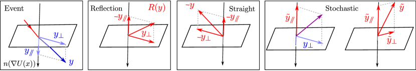
Figure 1: After an event, a new direction can be picked in a deterministic way (Reflection or Straight kernel) or, by exploiting the global symmetry around $\nabla U$, the new direction $\tilde{y}$ is picked randomly according to the decomposition of the kernel $Q$ into $K^{x,\sslash}$ and $K^{x,y_{\sslash},\perp}$. In the leftmost figure, $n(\nabla U(x))$ stands for the normalized vector $\nabla U(x)/\left\|\nabla U(x)\right\|$.

Following this remark, the repel kernel $Q$ effect is decomposed into two contributions: first the update of the direction component along the gradient $\nabla U$ and second the update of the orthogonal components. Informally, the Markov kernel $Q$ can be written as the composition of two Markov kernel $K^{x,\sslash}$ and $K^{x,y_{\sslash},\perp}$, respectively on $\mathbb{R}\times\mathcal{B}(\mathbb{R})$ and $\mathrm{span}(\nabla U(x))^{\perp}\times\mathcal{B}(\mathrm{span}(\nabla U(x))^{\perp})$ and for any $x\in\mathbb{R}^{d}$ and $y_{\sslash}\in\mathbb{R}$. At the event $S_{n+1}$ and given the value of the process $(X_{S_{n+1}},Y_{S_{n}})=(X_{S_{n}}+(S_{n+1}-S_{n})Y_{S_{n}},Y_{S_{n}})$, the new direction is then chosen as follows:

1. decompose $Y_{S_{n}}=Y_{S_{n}}^{\sslash}\nabla U(X_{S_{n+1}})+Y_{S_{n}}^{\perp}$ where $Y_{S_{n}}^{\perp}\in\mathrm{span}(\nabla U(x))^{\perp}$;

2. first sample $Y_{S_{n+1}}^{\sslash}\sim K^{X_{S_{n+1}},\sslash}(-Y_{S_{n}}^{\sslash},\cdot)$ and second $Y_{S_{n+1}}^{\perp}\sim K^{X_{S_{n+1}},Y_{S_{n+1}}^{\sslash},\perp}(Y_{S_{n}},\cdot)$;

3. set $Y_{S_{n+1}}=Y_{S_{n+1}}^{\sslash}\nabla U(X_{S_{n+1}})+Y_{S_{n+1}}^{\perp}$.

This decomposition for the repel kernel is illustrated on Figure 1 and the related pseudo-code simulating a PDMP based on such a choice for $Q$ is given in Algorithm 1.

Data: Markov kernels $\{(K^{x,y_{\sslash},\perp},K^{x,\sslash})\,:\,x\in\mathbb{R}^{d},\,y_{\sslash}\in\mathbb{R}\}$, refreshment rate $\bar{\lambda}\geq 0$ and initial points $(X_{0},Y_{0})$

Result: Generic PDMC $(X_{t},Y_{t})_{t\geq 0}$ based on Theorem 1

Initialize $S_{0}=0$ and a sequence of i.i.d. exponential random variables $(E_{i}^{\text{Ev}},E_{i}^{\text{Ref}})_{i\geq 1}$ with parameter $1$

Set $T_{1}^{\text{Ref}}=E^{\text{Ref}}_{1}/$ $\bar{\lambda}$ Time before refreshment

for $n\geq 0$ do

      Set $T_{n+1}^{\text{Ev}}=\inf\{t\geq 0\,:\,\int_{0}^{t}\left\langle Y_{S_{n}},\nabla U(X_{S_{n}}+uY_{S_{n}})\right\rangle_{+}\mathrm{d}u\geq E^{\text{Ev}}_{n+1}\}$ Time before event

      Set $T_{n+1}=\min(T_{n+1}^{\text{Ev}},T_{n+1}^{\text{Ref}})$ and $S_{n+1}=S_{n}+T_{n+1}$ Time before direction change

      Set $Y_{t}=Y_{S_{n}}$, $X_{t}=X_{S_{n}}+(t-S_{n})Y_{S_{n}}$ for $t\in\left(S_{n},S_{n+1}\right)$ Update the position

      Set $X_{S_{n+1}}=X_{S_{n}}+T_{n+1}Y_{S_{n}}$

      if $T_{n+1}=T_{n+1}^{\text{Ev}}$ then

           $Y_{S_{n}}^{\sslash}=\left\langle Y_{S_{n}},\nabla U(X_{S_{n+1}})\right\rangle$ decompose the direction

           $Y_{S_{n}}^{\perp}=\{\operatorname{Id}-\nabla U(X_{S_{n+1}})\nabla U(X_{S_{n+1}})^{\operatorname{T}}\}Y_{S_{n}}$ along $\nabla U(X_{S_{n+1}})$

           $Y_{S_{n+1}}^{\sslash}\sim K^{X_{S_{n+1}},\sslash}(-Y_{S_{n}}^{\sslash},\cdot)$

           $Y_{S_{n+1}}^{\perp}\sim K^{X_{S_{n+1}},Y_{S_{n+1}}^{\sslash},\perp}(Y_{S_{n}},\cdot)$

           set $Y_{S_{n+1}}=Y_{S_{n+1}}^{\sslash}\nabla U(X_{S_{n+1}})+Y_{S_{n+1}}^{\perp}$

           Set $T_{n+2}^{\text{Ref}}=T_{n+1}^{\text{Ref}}-T_{n+1}$ Update the time before refreshment

          

           else

                Set $Y_{S_{n+1}}\sim\mu_{\mathsf{Y}}$ Refresh the direction

                Set $T_{n+2}^{\text{Ref}}=E^{\text{Ref}}_{n+2}/$ $\bar{\lambda}$ Update the time before refreshment

                end if

               

                end for

Algorithm 1 Forward EC

Now, the invariance of the extended target distribution $\tilde{\pi}$ for $(P_{t})_{t\geq 0}$ enforced by (8) implies simple conditions on the families $\{K^{x,\sslash}\,:\,x\in\mathbb{R}^{d}\}$ and $\{K^{x,y_{\sslash},\perp}\,:\,x\in\mathbb{R}^{d},y_{\sslash}\in\mathbb{R}\}$. Consider the following two real distributions: $\mu_{\mathsf{Y}}^{\mbox{{$\sslash$}}}$ the distribution of the first component of $Y$ if $Y\sim\mu_{\mathsf{Y}}$ and $\rho$ the distribution with density $y_{\sslash}\mapsto(y_{\sslash})_{-}$ with respect to $\mu_{\mathsf{Y}}^{\mbox{{$\sslash$}}}$. The first condition we need to impose is that for any $x\in\mathbb{R}^{d}$,

$$\text{the distribution $\rho$ is invariant for $K^{x,\sslash}$}\;. 1$$ (C)

The second condition leads to consider for any $x\in\mathbb{R}^{d}$, the conditional distribution $\tilde{T}^{x,\perp}(y_{\sslash},\cdot)$ of the orthogonal projection of $Y\sim\mu_{\mathsf{Y}}$ on $\mathrm{span}(\nabla U(x))^{\perp}$, i.e. the distribution of $\{\operatorname{Id}-\nabla U(x)\nabla U(x)^{\operatorname{T}}\}Y$, given the component of $Y$ along $\nabla U(x)$ is equal to $y_{\sslash}$. The condition imposes then that for any $x\in\mathbb{R}^{d}$ and $y_{\sslash}\in\mathbb{R}$,

$$\text{ $\tilde{T}^{x,\perp}(y_{\sslash},\cdot)$ is invariant for the Markov kernel $K^{x,y_{\sslash},\perp}$}\;. 2$$ (C)

In summary, the condition (C$2$) codes for the fact that the components on $\mathrm{span}(\nabla U(x))$ did not trigger any event, so that their conditional distribution is still $\tilde{T}^{x,\perp}(y_{\sslash},\cdot)$. On the contrary, the direction component $y_{\sslash}$ is no longer distributed according to $\mu_{\mathsf{Y}}^{\mbox{{$\sslash$}}}$ but according to the reflected-event distribution $\rho$ defined in (C$1$). This result is formally stated in Theorem 1 in the supplementary document.

In the case $K^{x,\sslash}$ and $K^{x,y_{\sslash},\perp}$ are the identity kernels, i.e. $K^{x,\sslash}(y_{\sslash},\cdot)=\updelta_{y_{\sslash}}(\cdot)$ and $K^{x,y_{\sslash},\perp}(y_{\perp},\cdot)=\updelta_{y_{\perp}}(\cdot)$ for any $x,y_{\sslash},y_{\perp}$, then the PDMC obtained from Algorithm 1 recovers the BPS. But Theorem 1 implies many other possible choices for $K^{x,y_{\sslash},\perp}$ and $K^{x,\sslash}$, and therefore lead to a continuum of PDMC methods, forming the Forward event-chain Monte Carlo class. In the next subsections, we present possible choices for $K^{x,\sslash}$ and $K^{x,y_{\sslash},\perp}$ and motivate heuristically their efficiency. The key idea is to keep the need for refreshment and artificial noise to a minimum, by ensuring a maximal exploration through the new direction picks at events, as they are already necessary for correctness.

3.1 Choices of $K^{x,\sslash}$

A natural choice for $K^{x,\sslash}$, for $x\in\mathbb{R}^{d}$, is to simply choose the probability measure $\rho$, if this latter can be efficiently sampled. In that case, we refer to the resulting scheme as a direct sampling method. If $\mu_{\mathsf{Y}}$ is the uniform distribution over the $d$-dimensional sphere $\mathbb{S}^{d}$, $d\geq 2$, then using spherical coordinates, we have for all $\mathsf{A}\in\mathcal{B}(\mathbb{R})$,

$$\rho(\mathsf{A})=\int_{0}^{\uppi/2}\mathbbm{1}_{\mathsf{A}}(-\cos(\theta))\,\frac{\cos(\theta)\sin^{d-2}(\theta)}{d-1}\mathrm{d}\theta=\int_{-1}^{0}\mathbbm{1}_{\mathsf{A}}(v)\frac{(-v)(1-v^{2})^{(d-3)/2}}{d-1}\mathrm{d}v\;.$$ (11)

Therefore, $\rho$ can be efficiently sampled since if $V$ is a uniform random variable on $\left[0,1\right]$, then it is straightforward to verify that $(1-V^{2/(d-1)})^{1/2}$ has distribution $\rho$. In the case where $\mu_{\mathsf{Y}}$ is the $d$-dimensional standard Gaussian distribution, then it is easy to check that $\mathsf{A}\mapsto\rho(-\mathsf{A})$ is the $\chi$-distribution with $2$ degrees of freedom, as proposed by Vanetti et al. (2017) building on earlier version of this work, with $K^{x,y_{\sslash},\perp}=\operatorname{Id}$.

It is also possible to set $K^{x,\sslash}$ to be a Markov kernel defined by a Metropolis-Hastings algorithm designed to sample from $\rho$. In that case, we refer to the resulting scheme as a Metropolis sampling method. One such example would be a random walk or independent Metropolis-Hastings algorithm on $\left[-1,0\right]$ with Gaussian or uniform noise. Explicit expressions for the associated Markov kernels for $\mathsf{Y}=\mathbb{S}^{d-1}$ are given in the supplementary document Appendix B. The choices for $K^{x,\sslash}$ are naturally not bounded to these schemes. For instance, it is possible to define a mixture of kernels, as e.g. a direct-sampling kernel with an identity one.

3.2 Choices of $K^{x,y_{\sslash},\perp}$

A trivial choice is $K^{x,y_{\sslash},\perp}=\operatorname{Id}$, which is the case of the BPS and standard EC processes, but which both rely on a refreshment step. It can be advantageous to set $K^{x,y_{\sslash},\perp}$ differently in order to improve the exploration of the state space and to therefore insure the ergodicity of the process, while aiming at setting the refreshment rate $\bar{\lambda}$ in (4) to zero. We propose next several possibilities for $K^{x,y_{\sslash},\perp}$ for the specific case $\mathsf{Y}=\mathbb{S}^{d-1}$.

The idea is to rely on the randomization achieved on the parallel component by $K^{x,\sslash}$ to minimize at most the randomization on the orthogonal components. As, for any $x\in\mathbb{R}^{d}$, $y_{\sslash}\in\left[0,1\right]$, $\tilde{T}^{x,\perp}(y_{\sslash},\cdot)$ is rotation invariant, we characterize the various choices for $K^{x,y_{\sslash},\perp}$ by considering for any $x\in\mathbb{R}^{d}$ a probability distribution $\nu^{x}$ on the set of orthogonal transformations $\mathbf{O}^{x}$ on $\mathrm{span}(\nabla U(x))^{\perp}$ and define the Markov kernels for any $y_{\perp}\in\mathrm{span}(\nabla U(x))^{\perp}\setminus\{0\}$ and $\mathsf{A}\in\mathrm{span}(\nabla U(x))^{\perp}$ by

$$K^{x,y_{\sslash},\perp}_{\text{naive}}(y_{\perp},\mathsf{A}) =\int_{\mathbf{O}^{x}}\mathbbm{1}_{\mathsf{A}}\left((1-y_{\sslash}^{2})^{1/2}\mathrm{O}(y_{\perp}/\left\|y_{\perp}\right\|)\right)\mathrm{d}\nu^{x}(\mathrm{O})\;,$$ (12)

$$K^{x,y_{\sslash},\perp}_{\text{pos}}(y_{\perp},\mathsf{A}) =\int_{\mathbf{O}^{x}}\mathbbm{1}_{\mathsf{A}}\left((1-y_{\sslash}^{2})^{1/2}\operatorname{sign}(\left\langle y_{\perp},\mathrm{O}y_{\perp}\right\rangle)\mathrm{O}(y_{\perp}/\left\|y_{\perp}\right\|)\right)\mathrm{d}\nu^{x}(\mathrm{O})\;.$$ (13)

In the case $y_{\perp}=0$, just choose a deterministic point in the $d-1$-dimensional sphere of $\mathrm{span}(\nabla U(x))$. Both kernels then admit $\tilde{T}^{x,\perp}(y_{\sslash},\cdot)$ as invariant distribution for any $x\in\mathbb{R}^{d}$, $y_{\sslash}\in\left[0,1\right]$ when $\mu_{\mathsf{Y}}$ is the uniform distribution on $\mathbb{S}^{d-1}$. Indeed, the result for $K^{x,y_{\sslash},\perp}_{\text{naive}}$ is straightforward. As for $K^{x,y_{\sslash},\perp}_{\text{pos}}$, using that $\tilde{T}^{x,\perp}(y_{\sslash},\cdot)$ is rotation invariant, we get easily that $\tilde{T}^{x,\perp}(y_{\sslash},\cdot)K^{x,y_{\sslash},\perp}_{\text{pos}}$ is rotation invariant with support included in the $(d-1)$-dimensional sphere of $\mathrm{span}(\nabla U(x))^{\perp}$ with radius $(1-y_{\sslash}^{2})^{1/2}$, therefore $\tilde{T}^{x,\perp}(y_{\sslash},\cdot)K^{x,y_{\sslash},\perp}_{\text{pos}}=\tilde{T}^{x,\perp}(y_{\sslash},\cdot)$. Sampling from $K^{x,y_{\sslash},\perp}_{{\text{naive}}}(y_{\perp},\cdot)$ (resp. $K^{x,y_{\sslash},\perp}_{\text{pos}}(y_{\perp},\cdot)$) comes down to sampling $O$ from $\nu^{x}$ and set $Y_{\perp}=O(y_{\perp})$ (resp. $Y_{\perp}=\operatorname{sign}(\left\langle y_{\perp},O(y_{\perp})\right\rangle)O(y_{\perp})$). Contrary to $K^{x,y_{\sslash},\perp}_{{\text{naive}}}$, using $K^{x,y_{\sslash},\perp}_{\text{pos}}$ imposes that the new direction $Y_{\perp}$ satisfies $\left\langle y_{\perp},Y_{\perp}\right\rangle\geq 0$ and therefore avoids that the position backtracks. Finally, this description can be further generalized in the case of $\mu_{\mathsf{Y}}$ being the standard Gaussian distribution by adding an additional norm sampling step.

This class of Markov kernels $K^{x,y_{\sslash},\perp}$ offers a great freedom on the randomness we want to use in the algorithm and potentially avoid random-walk behaviour by changing a full and global refreshment into a sparse and orthogonal one. Indeed, if we choose for $\nu^{x}$, the uniform distribution on $\mathbf{O}^{x}$, then the noise produced by the method is significant. In fact, when $\mathsf{Y}=\mathbb{S}^{d-1}$, $K^{x,y_{\sslash},\perp}$ is equal to $T^{x,\perp}(y_{\sslash},\cdot)$ for any $x\in\mathbb{R}^{d}$ and $y_{\sslash}\in\left[-1,1\right]$. The resulting scheme is referred to as a full-orthogonal refresh method. In the case where $\mu_{\mathsf{Y}}$ is the $d$-dimensional standard Gaussian distribution, this choice of $K^{x,y_{\sslash},\perp}$ can be extended by a norm resampling to recover $T^{x,\perp}(y_{\sslash},\cdot)$. It was also proposed in Wu and Robert (2017), after earlier versions of this work, in the case where $K^{x,\sslash}=\operatorname{Id}$. However such a choice, while ensuring ergodicity (Wu and Robert, 2017), leads to a quasi-refreshment at every event and introduces strong noise and random-walk behavior, see e.g. Figure 14 in supplement. The noise can be reduced by considering a mixture with the identity kernel, but this asks for a fine tuning and is similar to choosing $K^{x,y_{\sslash},\perp}=\operatorname{Id}$ and $\bar{\lambda}\neq 0$, see Figures 18 and 20.

On the contrary, if we explore another strategy based on a kernel $K^{x,y_{\sslash},\perp}$ allowing only for a partial refreshment and choose for $\nu^{x}$ to be a probability measure such that its support is contained in the subspace of orthogonal matrices, $\mathbf{O}^{p}_{x}$, which only act on $p$-dimensional space, $p\in\{2,\ldots,d-1\}$, i.e.

$$\mathbf{O}^{p}_{x}=\left\{\mathrm{O}\in\mathbf{O}_{x}\,:\;\ker(\operatorname{Id}-\mathrm{O})=d-1-p\right\}\;,$$

then the noise can be considerably smaller taking for example $p=2$ and $d$ large. In addition, distributions on $\mathbf{O}^{p}_{x}$ can be very cheap to compute for small $p$ as we will see. In the case where $\nu^{x}$ is the uniform distribution on $\mathbf{O}^{p}_{x}$, the choice of $K^{x,y_{\sslash},\perp}=K^{x,y_{\sslash},\perp}_{{\text{naive}}}$ and $K^{x,y_{\sslash},\perp}=K^{x,y_{\sslash},\perp}_{\text{pos}}$ defined by (12) and (13) respectively, lead to scheme referred in the following as naive or positive $p$-orthogonal refresh.

From a practical perspective, distributions $\nu^{x}$ on $\mathbf{O}_{x}$ can be easily derived from a probability distribution on the set of orthogonal matrices $\mathbf{O}(d)$, with its Borel $\sigma$-field $\mathcal{B}(\mathbf{O}(d))$. Indeed, it suffices to compute an orthogonal basis for $\mathrm{span}(\nabla U(x))^{\perp}$ which can be done using the Gram-Schmidt process on the canonical basis $(\mathbf{e}_{i})_{i\in\{1,\ldots,d\}}$. An other solution, which is computationally cheaper, is to find $i\in\{1,\ldots,d\}$ such that $\mathbf{e}_{i}\not\in\mathrm{span}(\nabla U(x))$, and set

$$\tilde{\mathbf{e}}_{j}(x)=\left\{\operatorname{Id}-2(\nabla U(x)-\mathbf{e}_{i})(\nabla U(x)-\mathbf{e}_{i})^{\operatorname{T}}\right\}\mathbf{e}_{j}\;,\,\text{ for $j\in\{1,\ldots,d\}\setminus\{i\}$}\;.$$

Then, we can easily check, since $\operatorname{Id}-2(\nabla U(x)-\mathbf{e}_{i})(\nabla U(x)-\mathbf{e}_{i})^{\operatorname{T}}$ is an orthogonal matrix, that $(\tilde{\mathbf{e}}_{j}(x))_{j\in\{1,\ldots,d\}\setminus\{i\}}$ is an orthonormal basis of $\mathrm{span}(\nabla U(x))^{\perp}$. We can observe that this computation has complexity $O(d^{2})$ which can be prohibitive and that is why we propose different constructions of probability measures $\nu^{x}$ without this constraint.

For example, we consider in Section 4, the case where, for $x\in\mathbb{R}^{d}$, $\nu^{x}$ is the distribution of the random variable $O$ defined as follows. Consider two $d$-dimensional Gaussian random variables $G_{1}$ and $G_{2}$, and the two orthogonal vectors $e_{1}$ and $e_{2}$ in $\mathrm{span}(\nabla U(x))^{\perp}$ defined by the Gram-Schmidt process and based on $\tilde{G}_{1}=(\operatorname{Id}-\nabla U(x)\nabla U(x)^{\operatorname{T}})G_{1}$ and $\tilde{G}_{2}=(\operatorname{Id}-\nabla U(x)\nabla U(x)^{\operatorname{T}})G_{2}$, i.e.

$$e_{1}=\tilde{G}_{1}/\|\tilde{G}_{1}\|\;,\,\,e_{2}=(\tilde{G_{2}}-\langle e_{1},\tilde{G_{2}}\rangle e_{1})/\|\tilde{G_{2}}-\langle e_{1},\tilde{G_{2}}\rangle e_{1}\|\;.$$

Then, the random orthogonal transformation $O$ is defined by

$$O_{\theta}=\{\cos(\theta)e_{1}+\sin(\theta)e_{2}\}e_{1}^{\operatorname{T}}+\{\sin(\theta)e_{1}-\cos(\theta)e_{2}\}e_{2}^{\operatorname{T}}\;,$$ (14)

for $\theta\in\left[0,2\uppi\right]$, belongs to $\mathbf{O}^{2}_{x}$ almost surely. The choice of $\theta$ naturally impacts the randomization and the case $\theta=\uppi/2$ will be referred to as the orthogonal switch refresh and the case where the parameter $\theta$ can be itself random ran-p-orthogonal refresh.

In the case where $\mu_{\mathsf{Y}}$ is the $d$-dimensional standard Gaussian distribution, we can consider the auto-regressive kernel on $\mathrm{span}(\nabla U(x))^{\perp}$, defined for any $y_{\perp}\in\mathrm{span}(\nabla U(x))^{\perp}$ and $\mathsf{A}\in\mathcal{B}(\mathrm{span}(\nabla U(x))^{\perp})$ by

$$K^{x,y_{\sslash},\perp}(y_{\perp},\mathsf{A})=(2\uppi)^{-d/2}\int_{\mathbb{R}^{d}}\mathbbm{1}_{\mathsf{A}}\left(\rho y_{\perp}+\sqrt{1-\rho^{2}}(\operatorname{Id}-\nabla U(x)\nabla U(x)^{\operatorname{T}})\tilde{y}\right)\mathrm{e}^{-\left\|\tilde{y}\right\|^{2}/2}\mathrm{d}\tilde{y}\;,$$

where $\rho\in\left[0,1\right]$. In other word, starting from $y_{\perp}$, the component along $\mathrm{span}(\nabla U(x))^{\perp}$ of the new direction is set to be $\rho y_{\perp}+(1-\rho^{2})(\operatorname{Id}-\nabla U(x)\nabla U(x)^{\operatorname{T}})Y_{1}$, where $Y_{1}$ is a $d$-dimensional standard Gaussian random variable. The resulting PDMP-MCMC with $K^{x,\sslash}=\operatorname{Id}$ or $K^{x,\sslash}=\rho$ was proposed by Vanetti et al. (2017).

As for $K^{x,\sslash}$, $K^{x,y_{\sslash},\perp}$ can be a mixture of the identity kernel and a partial refreshment of the orthogonal components: $p_{r}\operatorname{Id}+(1-p_{r})\tilde{K}^{x,\perp}$ such that $p_{r}\in\left[0,1\right]$ and $\tilde{T}^{x,\perp}$ is invariant for $\tilde{K}^{x,\perp}$ for any $x\in\mathbb{R}^{d}$. This step corresponds to a transformation of the sampling $Y_{n+1}^{\perp}$ in Algorithm 1 into $Y^{\perp}_{n+1}=BY_{S_{n}}+(1-B)\tilde{Y}_{n+1}^{\perp}$, where $B$ is a Bernoulli random variable with parameter $p_{r}$ and $\tilde{Y}_{n+1}^{\perp}\sim\tilde{K}^{X_{S_{n+1}},\perp}(\mathrm{P}^{X_{S_{n+1}},\perp}(Y_{S_{n}}),\cdot)$.

3.3 About refreshment strategy

Choices of $K^{x,y_{\sslash},\perp}$ different from the identity corresponds to a partial refresh of the orthogonal components of the direction. However, it can be advantageous to not use this kind of refreshment at any events.

As proposed above, a first option is to choose a mixture with the identity kernel and to choose the parameter $p_{r}$ accordingly. It can be interesting to control the partial refreshment through the time parameter directly, as fixing a refreshment time to $\mathrm{T}$ can simplify implementation. A second option is thus as follows. First, we extend the state space $\mathsf{E}=\mathbb{R}^{d}\times\mathsf{V}$ to $\mathsf{E}\times\{0,1\}$ and consider two Markov kernels $Q_{0},Q_{1}$ on $\mathbb{R}^{2d}\times\mathcal{B}(\mathbb{R}^{d})$ associated with $K^{x,y_{\sslash},\perp}_{0},K^{x,y_{\sslash},\perp}_{1},K^{x,\sslash}_{0},K^{x,\sslash}_{1}$ satisfying the conditions of Theorem 1. We now consider the PDMP $(\bar{X}_{t},\bar{Y}_{t},\bar{B}_{t})_{t\geq 0}$ corresponding to the differential flow $\bar{\varphi}_{t}(x,y,b)=(x+ty,y,b)$ for any $(x,y,b)\in\mathsf{E}\times\{0,1\}$, event rate $\lambda$ given by (4) with $\bar{\lambda}=0$ and Markov kernel $\bar{Q}$ on $(\mathsf{E}\times\{0,1\})\times\mathcal{B}(\mathsf{Y}\times\{0,1\})$ defined for any $(x,y,b)\in\mathsf{E}\times\{0,1\}$, $\mathsf{A}\in\mathcal{B}(\mathsf{Y})$ by

$$\bar{Q}((x,y,b),\mathsf{A}\times\{1\})=Q_{b}((x,y),\mathsf{A})\;.$$

If $Q_{0}$ differs from the identity kernel, $Q_{1}$ is the identity kernel and the extra variable $(\bar{B}_{t})_{t\geq 0}$ is updated to $0$ every time $\mathrm{T}>0$. This method produces a partial refreshment through $Q_{0}$ at each event following directly an update of $b$. More details and a pseudocode for this PDMP can be found in Section C.1 in the supplement. In particular, Figure 10 shows that the same decorrelation is obtained from both strategies.

It is also possible to transform the stochastic refreshment step ruled by the Poisson process of rate $\bar{\lambda}$ by a refreshment process at every time $\mathrm{T}$ by considering a collection of PDMP of length $\mathrm{T}$ instead of a single PDMP. A pseudocode is given in Algorithm 4 in the supplement.

3.4 PDMC and Potential Factorization

When the potential $U$ can be written as a sum of terms, $U(x)=\sum_{i=1}^{d}U_{i}(x)$ or considering directly the decomposition of the gradient $\nabla U$ over the direction, it can be convenient to exploit this decomposition through the implementation of the factorized Metropolis filter (Michel et al., 2014), for example to exploit some symmetries of the problem or reduce the complexity (Michel et al., 2019). It finds its equivalent in PDMC by considering a superposition of Poisson processes (Peters and de With, 2012; Michel et al., 2014; Bouchard-Côté et al., 2018). The results developed in Section 3 can be generalized using this property, as we explain in more details in the supplement Section C.2.

4 Numerical Experiments

We restrict our numerical studies to the case $\mathsf{V}=\mathbb{S}^{d-1}$ and $\mu_{\mathsf{Y}}$ is the uniform distribution on $\mathbb{S}^{d-1}$. After specifying the comparison methods in Section 4.1, we consider four different types of target density $\pi$: ill-conditioned Gaussian distributions in Section 4.2, a Poisson-Gaussian Markov random field in Section 4.3, mixtures of Gaussian distributions in Section 4.4 and finally a posteriori distributions coming from logistic regression problems in Section 4.5.

Codes used for these numerical experiments are available at https://bitbucket.org/MNMichel/forwardec/src/master/.

4.1 Comparing schemes

Similarly to Bernard et al. (2009), Bouchard-Côté et al. (2018) and Bierkens et al. (2019), for a fixed test function $h$ and PDMC $(X_{t},Y_{t})_{t\in\left[0,t_{f}\right]}$ for a final time $t_{f}\geq 0$, we consider the estimator of $\int_{\mathbb{R}^{d}}h(x)\pi(x)\mathrm{d}x$, $\hat{h}_{n}=n^{-1}\sum_{i=1}^{n}h(X_{\delta i})$, where $n=\left\lfloor t_{f}/\delta\right\rfloor$ and $\delta$ is a fixed step-size. To compare the different schemes, we then consider different criteria. First, we define the autocorrelation function associated with $h$ at lag $k\in\mathbb{N}$ by $C_{h}(k)=(n-k)^{-1}\sum_{i=0}^{n-k-1}\{(h(X_{\delta i})h(X_{\delta(i+k)})-m_{h}^{2})/\sigma^{2}_{h}\}$, where $m_{h}$ and $\sigma_{h}$ are either set to $\int_{\mathbb{R}^{d}}h(x)\pi(x)\mathrm{d}x$ and $\int_{\mathbb{R}^{d}}(h(x)-m_{h})^{2}\pi(x)\mathrm{d}x$ when it is possible to calculate these values or to approximations of these quantities obtained after a long run. Other criteria that we investigate amongst the different schemes is their integrated correlation time, $\tau^{\mathrm{int}}_{h}$ defined by $\tau^{\mathrm{int}}_{h}=1/2+\sum_{k=1}^{N_{\mathrm{int}}}(1-k/N)C_{h}(k)$ where $N_{\mathrm{int}}=\inf\{k\in\mathbb{N}\,:\,\text{ for all }i\geq k,\,\left|C_{h}(i)\right|\leq 10^{-3}\}$, and their Effective Sample Size (ESS) given by $\mathrm{ESS}^{h}=N_{\tau_{\mathrm{int}}}/(2\tau^{\mathrm{int}}_{h})$. Finally, we stress the importance of using different test functions $h$ as PDMC, thanks to their ballistic trajectories, can lead to fast decorrelation for some functions $h$, while showing a very slow decay for others or even lack of ergodicity, see e.g. Figure 16 in the supplement.

To be able to have a fair comparison in terms of computational efficiency, we plot the autocorrelations as a function of the averaged number of events per samples $n_{\delta}$, corresponding to the averaged number of gradient evaluations per samples. In practice, it simply leads to the sequence $(C^{h}(k/n_{\delta}))_{k\in n_{\delta}\mathbb{N}}$. The same procedure is done for the integrated correlation time, which ends up being multiplied by $n_{\delta}$. Box plots are based on $100$ runs of $10^{5}$ samples separated by a fixed $\delta$ which will be specified.

In the following experiments, we compare the performance of the following schemes:

• Forward No Ref: direct-sampling scheme with no refreshment of the orthogonal components and $\bar{\lambda}=0$. This method corresponds to the choice of $K^{x,\sslash}=\rho$ and $K^{x,y_{\sslash},\perp}=\operatorname{Id}$ in Algorithm 1. As there is no refreshment, particular care on testing ergodicity of the process has to be taken.

• Forward All Ref: direct-sampling scheme with refreshment at every event according to an orthogonal switch and $\bar{\lambda}=0$. This method corresponds to the choice of $K^{x,\sslash}=\rho$ and $K^{x,y_{\sslash},\perp}=K^{x,y_{\sslash},\perp}_{\text{pos}}$ defined by (13), where $\nu^{x}$ is the distribution of the random variable defined by (14) with $\theta=\uppi/2$.

• Forward Ref: direct-sampling scheme with refreshment at an event every time $\mathrm{T}$ according to an orthogonal switch and $\bar{\lambda}=0$ see Section 3.3. This method corresponds to the pseudo-code Algorithm 3 in the supplementary document using the two kernels $Q_{0}$ and $Q_{1}$ associated with $K^{x,\sslash}_{0}=K^{x,\sslash}_{1}=\rho$ and $K^{x,y_{\sslash},\perp}_{0}=K^{x,y_{\sslash},\perp}_{\text{pos}}$ where $\nu^{x}$ is the distribution of the random variable defined by (14) with $\theta=\uppi/2$.

• Forward Full Ref: direct-sampling scheme with no refreshment of the orthogonal components and a full refreshment of the direction every $\mathrm{T}$, see Section 3.3. This method corresponds to Algorithm 4 in the supplementary document and to the choice $K^{x,\sslash}=\rho$, $K^{x,y_{\sslash},\perp}=\operatorname{Id}$.

• BPS Full Ref: reflection scheme with no refreshment of the orthogonal components and a full refreshment of the direction every $\mathrm{T}$, see Section 3.3. This method corresponds to Algorithm 4 and to the choice $K^{x,\sslash}=\operatorname{Id}$, $K^{x,y_{\sslash},\perp}=\operatorname{Id}$.

• BPS No Ref: reflection scheme ($K^{x,\sslash}=\operatorname{Id}$) with no refreshment of the orthogonal components ($K^{x,y_{\sslash},\perp}=\operatorname{Id}$) and no full refreshment ($\bar{\lambda}=0$). As there is no refreshment, particular care on testing ergodicity of the process has to be taken.

Out of completeness, we will also display the performance of the Hamiltonian Monte Carlo and the Zig Zag schemes for the anisotropic Gaussian experiments. As we are comparing the efficiency of given Markov kernels, we did not include schemes based on metric adaptations and fits, as NUTS (Hoffman and Gelman, 2014).

4.2 Anisotropic Gaussian distribution

We consider the problem of sampling from a $d$-dimensional zero-mean anisotropic Gaussian distribution in which the eigenvalues of the covariance matrix $\Sigma$ are log-linearly distributed between $1$ and $10^{6}$, such as in Sohl-Dickstein et al. (2014), i.e.  we set for any $i,j\in\{1,\ldots,d\}$, and $d\geq 2$,

$$\Sigma_{i,j}=\updelta_{i,j}\exp\left(\frac{6(i-1)}{d-1}\log 10\right)\;.$$ (15)

We develop the calculations of the event times for a Gaussian distribution in Section C.3 of the supplement.

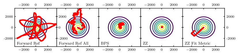
Figure 2: First $1000$ samples (red crosses) for the $400$-dimensional zero-mean Gaussian distribution with covariance matrix given by (15) (contoured) generated from the same initial position. Successive positions are separated by the same number of events ($\sim 55$).

We tuned the refreshment rate for Forward Ref and BPS Full Ref in order to achieve the fastest decorrelation for the potential $U$ at $d=400$ ($T=500$, corresponding roughly to an average of $55$ events), as $U$ is not sensitive to the ill-conditioned nature of the distribution and requires mixing on all dimensions. To allow for an easy comparison with BPS, Forward Full Ref refreshment rate is also set to the same rate. The Hamiltonian Monte Carlo scheme is optimized through an adaptive implementation in order to achieve an acceptance rate $\approx 0.6$ (Beskos et al., 2013). The ZZ algorithm is run according to a random basis of vectors (ZZ) and to the eigenvectors basis (ZZ Fit Metric). We also simulated a standard EC scheme factorized according to the eigenvector basis and refer to it in the following by Optimized EC, playing the role of an ideal reference. The difference between the EC and ZZ schemes lies in the fact that the EC successively updates the position according to each basis vector successively, whereas the ZZ updates the position according to all simultaneously. Finally, for this highly-symmetrical distribution, the schemes without refreshment (BPS No Ref and Forward No Ref) are not ergodic, as they would stick to a plane. Comparison to a standard Hastings-Metropolis scheme can be found in the supplement in Section D.1, showing the limited efficiency of a standard random walk for this type of distribution.

Figure 2 exhibits section plots showing the first $1000$ samples generated from an initial position at the origin. This qualitative picture is confirmed by the autocorrelation functions displayed on Figure 3 for the reflection-kernel schemes (HMC included) and on Figure 4 for the straight-kernel schemes and the scaling of integrated autocorrelation times with the dimension in Figure 5, in terms of events and of CPU times, to account for extra complexities, as in particular for the ZZ scheme in the general case. The corresponding fit results are given in Table 1.

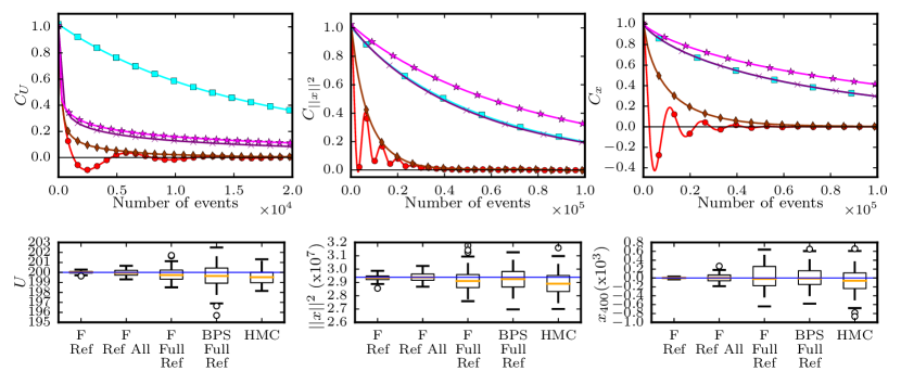
Figure 3: Top: Autocorrelation functions $C$ of $U$ (Left), $\left\|x\right\|^{2}$ (Middle) and $x$ (Right) for the zero-mean Gaussian distribution with covariance matrix given by (15) and $d=400$ for Forward Ref (red, circles), Forward Ref All (maroon, thin diamond), Forward Full Ref (purple, cross), BPS Full Ref (cyan, square) and HMC (magenta, star).Bottom: Boxplots for $U$, $\left\|x\right\|$ and highest-variance component $x_{400}$. For the box plots, samples are separated by an averaged of $55$ events (or gradient evaluations for HMC).

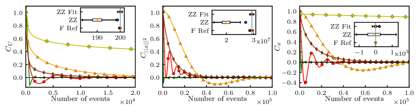
Figure 4: Autocorrelation functions $C$ of $U$ (Left), $\left\|x\right\|^{2}$ (Middle) and $x$ (Right) for the zero-mean Gaussian distribution with covariance matrix given by (15) and $d=400$. for Forward Ref (red, circles), Forward Ref All (maroon, thin diamond), ZZ (light green, diamond), ZZ Fit Metric (yellow, up triangle) and Optimized EC (green, right triangle). The autocorrelation function of the norm for ZZ is not displayed out of convergence issue. The insets are the respective boxplots for $U$, $\left\|x\right\|$ and highest-variance component $x_{400}$. For the box plots, samples are separated by an averaged of $55$ events.

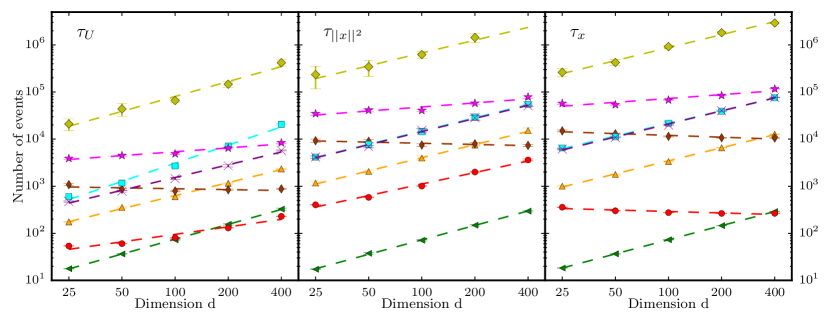
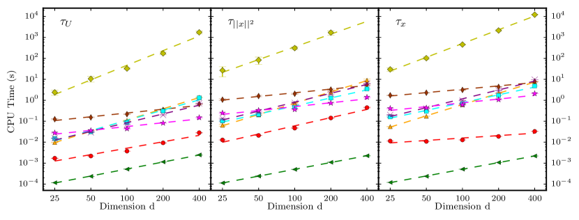
Figure 5: Integrated autocorrelation times $\tau$ of $U$ (Left), $\left\|x\right\|^{2}$ (Middle) and $x$ (Right) for the zero-mean Gaussian distribution with covariance matrix given by (15) for Forward Ref (red, circles), Forward Ref All (maroon, thin diamond), Forward Full Ref (purple, cross), BPS Full Ref (cyan, square), HMC (magenta, star) ZZ (light green, diamond), ZZ Fit Metric (yellow, up triangle) and Optimized EC (green, right triangle), in number of events (Top) and amount of CPU time (Bottom). Dashed lines stand for the fit $\tau_{h}=Ad^{z}$. Error bars may be covered by the markers.

In summary, Forward Ref achieves clear quantitative acceleration in comparison to the other methods, excluding the ideal Optimized EC, and exhibits antithetic autocorrelations, showing the reduction of any random-walk behavior. Moreover, as the scaling with the dimension $d$ is smaller than for the other methods excepted HMC and Forward All Ref), this acceleration increases with the dimension of the target distribution. Forward All Ref exhibits the smallest scaling, $0$ in terms of number of events and $0.6$ in terms of CPU time, matching then HMC. This acceleration is due to both the direct-sampling $K^{x,\sslash}$ and the sparse orthogonal switch $K^{x,y_{\sslash},\perp}$. Forward Full Ref has the same $K^{x,\sslash}$ than Forward Ref and Forward Ref All but a different $K^{x,y_{\sslash},\perp}$ and exhibits a fast decorrelation of $U$ compared to BPS, but is overall slower than Forward Ref and Forward Ref All. Even set to an optimal refreshment time $\mathrm{T}$ > 0, BPS is slower and, set to an identic sparse orthogonal switch $K^{x,y_{\sslash},\perp}$, converges even more slowly, see in the supplement Section D.3 and Figure 16. Finally, regarding tuning sensitivity, the parameter-free version, Forward Ref All, shows an even better scaling than Forward Ref while requiring no tuning, which makes it a competitive option for high dimensions. The refreshment time $\mathrm{T}$ requires indeed no crucial tuning for Forward Ref, on the contrary of BPS or Forward Full Ref, as illustrated by Figure 17, Figure 18 and Figure 19 in supplement, which show that varying $\mathrm{T}$ from $50$ to $1000$ leads up to more than a $30-$fold increase of the maximal integrated autocorrelation time for BPS and Forward Full Ref, whereas it is less than a $4-$fold increase for Forward Ref. The impact of the choice of $p$ and $\theta$ in $K^{x,y_{\sslash},\perp}$ are also investigated in Appendix D.4 and appears not to be critical.

Table 1: Scaling $z$ of the integrated autocorrelation times $\tau_{h}$ with the dimension of the anisotropic Gaussian distribution in terms of events (Top) or CPU time (Bottom), for the least-squares fit $\tau_{h}=Ad^{z}$ by Levenberg-Marquardt gradient method.

Events	F. Ref	F. Ref All	F. Full	BPS Full	ZZ	ZZ Fit	HMC	Opt. EC
$U$	0.53$\pm$0.01	-0.06$\pm$0.02	0.90$\pm$0.01	1.28$\pm$0.02	1.05$\pm$0.06	0.92$\pm$0.01	0.27$\pm$0.02	1.05$\pm$0.01
$\left\|x\right\|^{2}$	0.81$\pm$0.01	-0.08$\pm$0.03	0.93$\pm$0.03	0.93$\pm$0.02	0.9$\pm$0.3	0.93$\pm$0.05	0.28$\pm$0.04	1.02$\pm$0.01
$x$	-0.10$\pm$0.01	-0.13$\pm$0.01	0.92$\pm$0.01	0.89$\pm$0.01	0.92$\pm$0.09	0.92$\pm$0.01	0.27$\pm$0.02	1.00$\pm$0.01
CPU	F. Ref	F. Ref All	F. Full	BPS Full	ZZ	ZZ Fit	HMC	Opt. EC
$U$	1.00$\pm$0.01	0.60$\pm$0.02	1.39$\pm$0.02	1.62$\pm$0.02	2.3$\pm$0.1	1.78$\pm$0.01	0.60$\pm$0.02	1.1$\pm$0.01
$\left\|x\right\|^{2}$	1.30$\pm$0.01	0.60$\pm$0.03	1.41$\pm$0.03	1.28$\pm$0.02	2.0$\pm$0.3	1.79$\pm$0.05	0.61$\pm$0.04	1.08$\pm$0.01
$x$	0.35$\pm$0.01	0.53$\pm$0.01	1.40$\pm$0.01	1.23$\pm$0.01	2.2$\pm$0.1	1.79$\pm$0.01	0.60$\pm$0.01	1.05$\pm$0.01

Additional numerical experiments have been conducted to study other choices of $K^{x,\sslash}$ and $K^{x,y_{\sslash},\perp}$ for a Forward scheme and can be found in the supplement, Section D.2 and Section D.3. They show that Forward Ref is one of the most efficient tested schemes, that a direct Forward EC with a full-orthogonal refreshment every $\mathrm{T}$ is similar to Forward Full Ref and that sparse-orthogonal refreshment schemes are more robust to the choice of $\mathrm{T}$ for the refreshment than a full-orthogonal one.

4.3 Poisson-Gaussian Markov random field

To assess the performance for more complex models, we now consider a Poisson-Gaussian Markov random field model similarly to (Bouchard-Côté et al., 2018, Section 4.5). In this setting, the observations $\mathbf{Y}=(Y_{i,j})_{(i,j)\in\{1,\ldots,\tilde{d}\}^{2}}\in\mathbb{N}^{\tilde{d}^{2}}$ are supposed to be independent samples such that for any $(i,j)\in\{1,\ldots,\tilde{d}\}^{2}$, $Y_{i,j}$ has a Poisson distribution with parameter $\exp(x_{i,j})$ with $x\in\mathbb{R}$. The parameter $\mathbf{x}=(x_{i,j})_{(i,j)\in\{1,\ldots,\tilde{d}\}^{2}}$ is assumed to be a Gaussian random field, i.e. the prior distribution is set to be the zero-mean Gaussian distribution with covariance matrix $\tilde{\Sigma}_{(i,j),(\tilde{i},\tilde{j})}=\exp(-(2\upsigma^{2})^{-1}\{(i-j)^{2}+(\tilde{i}-\tilde{j})^{2}\}^{1/2})$, and $\upsigma^{2}=\tilde{d}-1$. The target distribution $\pi$ admits a potential $U$ given for any $\mathbf{x}\in\mathbb{R}^{\tilde{d}^{2}}$ by

$$U(\mathbf{x})=\frac{1}{2}\sum_{i,j,\tilde{i},\tilde{j}=1}^{\tilde{d}}x_{i,j}\tilde{\Sigma}_{(i,j),(\tilde{i},\tilde{j})}^{-1}x_{\tilde{i},\tilde{j}}+\sum_{i,j=1}^{\tilde{d}}\{\exp(x_{i,j})-Y_{i,j}x_{i,j}\}\;.$$

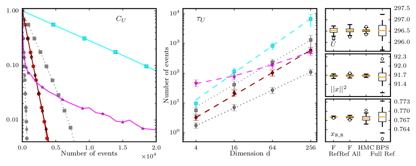
Figure 6: Left: Autocorrelation functions $C_{U}$ for the potential U for $d=256$ for HMC (magenta, star), Forward Ref (red, circle), Forward Ref All (maroon, diamond) and BPS Full Ref (cyan, square). Middle: Scaling with $d$ of the integrated autocorrelation times $\tau$ of $U$ for the same schemes. For both $C_{U}$ and $\tau$, the time unit is the number of gradient evaluations or events. The jump times/true events of the PDMC are computed through thinning and required several fake events, results in terms of true events/jump times are represented with a dotted grey line and with the respective markers. Right: Boxplots for $U$, $\left\|x\right\|^{2}$ and $x_{88}$ at $d=256$. For the box plots, samples are separated by the same averaged CPU times ($\sim 1.10^{-3}s$), resulting in average to 500 gradient evaluations for HMC and from 137 (Forward) to 155 (BPS) events for PDMC schemes per sample.

We compared the schemes Forward Ref, Forward Ref All, HMC and BPS for the dimensions $d=\tilde{d}^{2}\in\{4,16,64,256\}$. The refreshment time is set to $T=5$ for Forward Ref and to $T=2$ for BPS. This choice achieves the fastest decorrelation in $U$, which appears to be the slowest observable to converge, in comparison to $\left\|\mathbf{x}\right\|^{2}$ and $\mathbf{x}$. The event times of the underlying PDMP are computed through the decomposition and thinning of the target Poisson process. We refer to Section C.4 in the supplement for details on this procedure and to Michel et al. (2014) and Bouchard-Côté et al. (2018).

Table 2: Scaling $z$ of the integrated autocorrelation times $\tau_{U}$ with the dimension $d$ in the Poisson-Gaussian Markov random field model, for the least-squares fit $\tau_{U}=Ad^{z}+B$ by Levenberg-Marquardt gradient method. For PDMC schemes, results are given in terms of gradient evaluations/all events, jump times/true events and CPU times, for HMC, in terms of gradient evaluations/leapfrogs and CPU times.

F. Ref			F. Ref All			BPS Full			HMC
All Ev.	True Ev.	CPU	All Ev.	True Ev.	CPU	All Ev.	True Ev.	CPU	Grad. Eval	CPU
1.27$\pm$0.10	1.00 $\pm$0.05	2.4 $\pm$0.1	1.27$\pm$0.10	1.00 $\pm$0.05	2.3 $\pm$0.1	1.5$\pm$0.1	1.25 $\pm$0.10	3.1 $\pm$0.1	0.8$\pm$0.1	2.3 $\pm$0.1

Figure 6 displays the autocorrelation functions and the integrated autocorrelation times for the potential $U$ obtained from the different schemes. The fitted scaling of the latter with the dimension $d$ can be found in Table 2. In addition, Figure 6 also exhibits boxplots for $U$, the norm $\left\|\mathbf{x}\right\|^{2}$ and the component $x_{8,8}$ for $d=256$. First, as the event times are computed through a thinning procedure, it leads to an extra computational cost compared to a direct computation, if it was available. Then, the results show that BPS is outperformed in all situation. Forward Ref and Forward Ref All behaves in the same manner, confirming that the refreshment tuning for Forward Ref schemes is also not crucial in that case. HMC, if displaying slower decorrelations than Forward-type schemes, shows a better scaling, except when given in CPU time. Finally, from the boxplots, Forward-type schemes seems to be the more efficient for the component $x_{8,8}$ and as efficient as HMC for the norm.

4.4 Mixture of Gaussian distributions

Our next numerical experiment is based on the sampling of a mixture of $5$-Gaussian distributions of dimension $d$ to test whether a direct-sampling scheme could lead to difficulties to get out of a local mode. In order to introduce some randomness, a set of $d$ random numbers $(\sigma^{2}_{i})_{i\in\{1,\ldots,d\}}$ is picked uniformly between $0.5$ and $3$. Then for $j\in\{1,\ldots,5\}$, we consider the Gaussian distribution with mean $\mu_{j}$ and covariance matrix $\Sigma_{j}$ where $\Sigma_{j}=\mathrm{diag}(\sigma_{\kappa_{j}(1)}^{2},\ldots,\sigma_{\kappa_{j}(d)}^{2})$, where $(\kappa_{j})_{j\in\{1,\ldots,5\}}$ is a sequence of $5$ uniformly-random permutations of $\{1,\ldots,d\}$, therefore $(\Sigma_{j})_{j\in\{1,\ldots,N\}}$ are equal up to a rotation. The mean are defined recursively by $\mu_{j}=0$ if $j=1$ and for $j>1$ by $\mu_{j}=\mu_{j-1}+(\nu_{1}\sigma_{\kappa_{j}(i)}+\nu_{2}\sigma_{\kappa_{j-1}(i)})^{\top}_{i\in\{1,\ldots,d\}}$, where $\nu_{1},\nu_{2}$ are uniform samples between $1$ and $2$. This choice has been made to ensure a separation between each mode of at least both standard deviations. Each Gaussian distribution has equal probability in the mixture. The event time can be computed through a thinning procedure, as done in (Wu and Robert, 2017, Example 2).

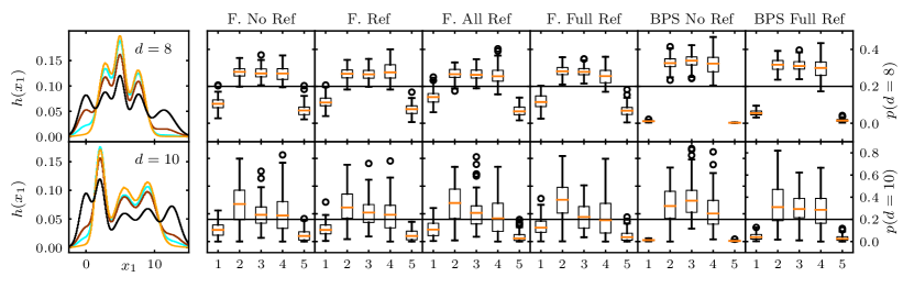
Figure 7: Histograms of component $x_{1}$ for the Gaussian Mixtures in dimension $d=8$ (Top Left) and $d=10$ (Bottom Right) with, ordered from darker to lighter colors, real distributions (black), Forward Ref All (maroon), BPS No Ref (orange) and BPS Full Ref (cyan). The right panel shows the boxplots of the estimated mixture probabilities for $d=8$ (Top) and $d=10$ (Bottom) for different schemes.

In small dimensions ($d=2,4,5$), all the tested schemes give similar results in terms of efficiency, as exhibited by the ESS of the vector $x$ and the square norm $\left\|x\right\|^{2}$ in Table 4 in the supplementary. Contrary to the former Gaussian distribution, Forward No Ref and BPS No Ref appear to be ergodic. A sharp drop in the ESS can be observed between $d=2$ and $d=4$, especially for BPS No Ref, and, in higher dimensions ($d=8,10$), convergence is very slow. Refreshment time is tuned to $\mathrm{T}=100$ ($\sim 40$ events). We display in Figure 7 the histograms of the first component of $x$ averaged on $100$ runs of $4\times 10^{6}$ events and started from random initial positions drawn from the real distribution. Forward Ref All shows a better exploration than BPS Full Ref and BPS No Ref. This result is confirmed by the boxplots of the estimated mixture probabilities, obtained by assigning each successive sample of each run to a distribution based on the closest mean. Here runs were all started from $0$. A clear difference can be observed between Forward schemes and BPS schemes, as they share inside their class similar results in terms of exploration of the extreme modes, despite different refreshment schemes. BPS Full Ref shows a better exploration than BPS No Ref though. All in all, Forward methods do outperform BPS ones, the most efficient being Forward Ref All.

4.5 Logistic regression

We focus in this Section on a Bayesian logistic regression problem. The data $(y_{i})_{i\in\{1,\ldots,N\}}$, $N\in\mathbb{N}^{*}$, are assumed to be i.i.d. Bernouilli random variables with probability of success $\mathrm{logit}(\left\langle x_{i},\theta\right\rangle)$ for any $i\in\{1,\ldots,N\}$, where $(x_{i})_{i\in\{1,\ldots,N\}}$ are covariate variables, $\theta$ is the parameter of interest and $\mathrm{logit}(u)=\mathrm{e}^{u}/(1+\mathrm{e}^{u})$, for any $u\in\mathbb{R}$. The prior distribution on $\theta$ is assumed to be the $d$-dimensional zero-mean Gaussian distribution with covariance matrix $1000\times\mathrm{I}_{d}$. Then, the a posteriori distribution for this model has a potential given for any $\theta\in\mathbb{R}^{d}$ by

$$U(\theta)=\sum_{i=1}^{N}\left\{-y_{i}\left\langle x_{i},\theta\right\rangle+\log\left[1+\exp(\left\langle x_{i},\theta\right\rangle)\right]\right\}+\left\|\theta\right\|^{2}/(2\varsigma^{2})\;,\,\varsigma^{2}=1000\;.$$ (16)

We perform our numerical studies on the German credit dataset ($N=1000$, $d=25$) and Musk dataset ($N=476$, $d=167$) from the UCI repository Dua and Efi (2017). The procedure we follow for this example has been proposed in Michel et al. (2014) and (Bouchard-Côté et al., 2018, Section 3), and uses a decomposition of the gradient of the potential over the data. We refer to Section C.2 in the supplement for more details.

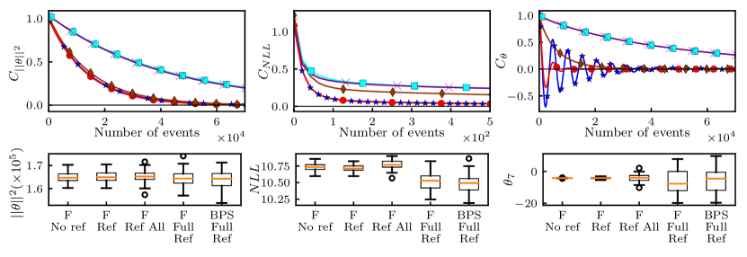
Figure 8: Top: Autocorrelation functions for the squared norm of the weights $\left\|\theta\right\|^{2}$ (left), the negative loglikelihood (NLL, middle) and $\theta$ (right) for the Musk dataset for Forward No Ref (blue, star), Forward Ref (red, circle), Forward Ref All (maroon, diamond), Forward Full Ref (purple, cross) and BPS Full Ref (cyan, square). Bottom: Boxplots for $\left\|\theta\right\|^{2}$, NLL and $\theta_{7}$, component with the highest variance.

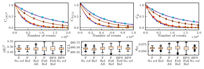
Figure 9: Top: Autocorrelation functions for the squared norm of the weights $\left\|\theta\right\|^{2}$ (left), the negative loglikelihood (NLL, middle) and $\theta$ (right) for German Credit dataset for Forward No Ref (blue, star), Forward Ref (red, circle), Forward Ref All (maroon, diamond), Forward Full Ref (purple, cross), BPS Full Ref (cyan, square) and BPS No Ref (yellow, up triangle). Bottom: Boxplots for $\left\|\theta\right\|^{2}$, NLL and $\theta_{21}$, component with the highest variance.

Table 3: ESS for the Musk and German credit datasets per event.

	Musk dataset			German credit dataset
Algorithm	$\theta$	$\left\|\theta\right\|^{2}$	NLL	$\theta$	$\left\|\theta\right\|^{2}$	NLL
Forward No Ref	240$\pm$80	4.3$\pm$0.1	228$\pm$10	160.0$\pm$0.8	145$\pm$3	324$\pm$5
Forward Ref	128$\pm$6	4.57$\pm$0.09	234$\pm$10	140.2$\pm$0.8	137$\pm$3	288$\pm$5
Forward Ref All	9.0$\pm$0.1	3.7$\pm$0.1	77$\pm$4	64.9$\pm$0.7	73$\pm$2	157$\pm$4
Forward Full Ref	1.03$\pm$0.02	1.23$\pm$0.08	20$\pm$1	34.5$\pm$0.9	44$\pm$1	107$\pm$3
BPS No Ref	–	–	–	149.7$\pm$0.7	143$\pm$3	282$\pm$5
BPS Full Ref	1.07$\pm$0.02	1.23$\pm$0.07	20$\pm$1	35.4$\pm$0.7	40$\pm$2	96$\pm$3

NOTE: All results are multiplied by $10^{5}$.

The refreshment time is fixed to $\mathrm{T}=10$ for the Musk dataset, corresponding to an average of $22$ events for Full Ref schemes, $21$ otherwise and to $\mathrm{T}=0.1$ for the German Credit dataset, corresponding to an average of $13$ events for Full Ref schemes, $12$ otherwise. Both BPS No Ref and Forward No Ref were also tested but BPS No Ref appears not to be ergodic on the Musk dataset, whereas no ergodicity issue were encountered with Forward No Ref. The autocorrelation functions for $\left\|\theta\right\|^{2}$, the negative loglikelihood and $\theta$ are shown in Figure 8 for the Musk dataset and in Figure 9 for the German Credit dataset. Forward Full Ref and BPS Full Ref have matching decorrelations on both datasets, as Forward Ref and Forward No Ref (except for the decorrelation of $\theta$ for the Musk dataset). We can observe that Forward schemes based on an orthogonal switch or no refreshment are faster and display their robustness to the refreshment-time tuning, as the decorrelation decay is always stronger from Forward No Ref to Forward Ref All. Quantitative accelerations can be found by comparing the ESS summarized in Table 3.

5 Conclusion

In this paper, we have introduced a generalized class of PDMC, Forward event-chain Monte Carlo, by exploiting the rotation symmetry around the gradient and relying on a global stochastic picture. The main practical asset is its flexibility, as it gives new possibilities in terms of refreshment and new-direction sampling schemes, while no requiring any crucial fine-tuning. By breaking free from quasi iso-potential trajectories, it allows to reduce the need for extra randomization and improves the efficiency of the exploration. Our numerical experiments also show that standard PDMC benefit from only transitioning to the Forward global stochastic direction sampling, while keeping the same refreshment scheme. Again, we stress that the stochastic direction sampling at event is required for correctness and is not equivalent to some artificial refreshment, the latter easily leading to a random-walk behavior.

In practice, we presented a collection of refreshment and new-direction sampling schemes which proved to bring accelerations in practice. There are however many possible other choices and a promising research axis lies in a quantitative theoretical study of the optimal refreshment scenario, depending on the problem at hand. A first question is how one can use the target geometry to determine which kernels to implement locally. Another line of research is to explore the impact of different choices of differential flows $\phi$ and function rates $\lambda$ than the ones considered here. To conclude, while PDMC appear as an exciting new MCMC development, a complete theoretical understanding is lacking and a key issue is indeed how to find the correct trade off between a diffusive exploration and a non-ergodic ballistic one.

Appendix A Formal derivation of new Markov kernels $Q$

We introduce the extended generator $\mathcal{A}$ (see (Davis, 1993, Theorem 26.14)) associated with the PDMP semi-group $(P_{t})_{t\geq 0}$ described in Section 2.2 with $\varphi$ and $\lambda$ given by (3) and (4). It is the operator $\mathcal{A}$ defined for all $f\in\mathrm{C}^{1}_{c}(\mathbb{R}^{2d})$ and $(x,y)\in\mathbb{R}^{2d}$ by

$$\mathcal{A}f(x,y)=\left\langle y,\nabla_{x}f(x,y)\right\rangle+\left\langle y,\nabla U(x)\right\rangle_{+}\left\{\int_{\mathbb{R}^{d}}f(x,\tilde{y})Q((x,y),\mathrm{d}\tilde{y})-f(x,y)\right\}\\ +\bar{\lambda}\left\{\int_{\mathbb{R}^{d}}f(x,\tilde{y})\mathrm{d}\mu_{\mathsf{Y}}(\tilde{y})-f(x,y)\right\}\;,$$ (17)

where $\mathrm{C}^{1}_{c}(\mathbb{R}^{2d})$ are the set of differentiable function from $\mathbb{R}^{2d}$ to $\mathbb{R}$ with compact support. Then by (Ethier and Kurtz, 1986, Proposition 9.2), for $\tilde{\pi}$ to be an invariant measure for $(X_{t},Y_{t})_{t\geq 0}$, it turns out that it is necessary that for all $f\in\mathrm{C}^{1}_{c}(\mathbb{R}^{2d})$,

$$\int_{\mathbb{R}^{d}\times\mathbb{R}^{d}}\mathcal{A}f(x,y)\mathrm{e}^{-U(x)}\mathrm{d}x\,\mathrm{d}\mu_{\mathsf{Y}}(y)=0\;.$$

By integration by part and elementary algebra based on (4), (5) and (17), this condition is equivalent to, for all $f\in\mathrm{C}^{1}_{c}(\mathbb{R}^{2d})$

$$\int_{\mathbb{R}^{d}\times\mathbb{R}^{d}}\int_{\mathbb{R}^{d}}\left\langle y,\nabla U(x)\right\rangle_{+}f(x,\tilde{y})Q((x,y),\mathrm{d}\tilde{y})\mathrm{e}^{-U(x)}\mathrm{d}x\mathrm{d}\mu_{\mathsf{Y}}(y)\\ =\int_{\mathbb{R}^{d}\times\mathbb{R}^{d}}\left\langle\tilde{y},\nabla U(x)\right\rangle_{-}f(x,\tilde{y})\mathrm{e}^{-U(x)}\mathrm{d}x\mathrm{d}\mu_{\mathsf{Y}}(\tilde{y})\;.$$

Furthermore, using Fubini’s theorem, this relation holds if the following condition is satisfied for almost all $x\in\mathbb{R}^{d}$,

$$\int_{\mathbb{R}^{d}}\int_{\mathbb{R}^{d}}\left\langle y,\nabla U(x)\right\rangle_{+}f(x,\tilde{y})Q((x,y),\mathrm{d}\tilde{y})\mathrm{d}\mu_{\mathsf{Y}}(y)=\int_{\mathbb{R}^{d}}\left\langle\tilde{y},\nabla U(x)\right\rangle_{-}f(x,\tilde{y})\mathrm{d}\mu_{\mathsf{Y}}(\tilde{y})\;.$$ (18)

As $\mu_{\mathsf{Y}}$ is rotation invariant, (18) is equivalent to the fact that for all $x\in\mathbb{R}^{d}$, such that $\nabla U(x)\not=0$, the probability measure defined for all $\mathsf{A}\in\mathcal{B}(\mathbb{R}^{d})$ by

$$\mu_{\mathrm{p}}^{x}(\mathsf{A})=\left.\int_{\mathbb{R}^{d}}\mathbbm{1}_{\mathsf{A}}(\tilde{y})\left\langle\tilde{y},\nabla U(x)\right\rangle_{-}\mu_{\mathsf{Y}}(\mathrm{d}\tilde{y})\middle/\int_{\mathbb{R}^{d}}\left\langle\tilde{y},\nabla U(x)\right\rangle_{-}\mu_{\mathsf{Y}}(\mathrm{d}\tilde{y})\right.\;,$$ (19)

is invariant for the Markov kernel on $\mathbb{R}^{d}\times\mathcal{B}(\mathbb{R}^{d})$, $(y,\mathsf{A})\mapsto RQ((x,y),\mathsf{A})$ where $R$ is the extended Reflection kernel on $\mathbb{R}^{2d}\times\mathcal{B}(\mathbb{R}^{2d})$ defined for all $(x,y)\in\mathbb{R}^{2d}$ by $R((x,y),\cdot)=\updelta_{(x,\phi_{R}(x,y))}(\cdot)$, where $\phi_{R}$ is defined in (10). Simply put, $\mu_{\mathrm{p}}^{x}$ is the reflected-event distribution, the probability distribution for the reflection of the new direction to trigger an event. From this observation, we derive a necessary general expression for the Markov kernel $Q$. In (18), $x\in\mathbb{R}^{d}$ is assumed to be fixed and if $\nabla U(x)=0$, then any choice of $Q$ is suitable and we choose $Q((x,y),\cdot)=\mu_{\mathsf{Y}}$. We consider now the case $x\in\mathbb{R}^{d}$ satisfies $\nabla U(x)\not=0$. The projection on $\nabla U(x)$ is essential in (18) and that is why we disintegrate $\mu_{\mathsf{Y}}$ accordingly. A global symmetry around $\nabla U$ then appears and circumvents any introduction of additional symmetry. More precisely, we define the map $\mathrm{P}^{x,\sslash}:\mathbb{R}^{d}\to\mathbb{R}$, $\mathrm{P}^{x,\perp}:\mathbb{R}^{d}\to\mathrm{span}(\nabla U(x))^{\perp}$ for all $y\in\mathbb{R}^{d}$ by $\mathrm{P}^{x,\sslash}(y)=\left\langle y,\mathrm{n}(x)\right\rangle$, and $\mathrm{P}^{x,\perp}(y)=\{\operatorname{Id}-\mathrm{n}\left(x\right)\mathrm{n}(x)^{\operatorname{T}}\}y$. In addition, consider the pushforward measure of $\mu_{\mathsf{Y}}$ by $\mathrm{P}^{x,\sslash}$ given for all $\mathsf{A}\in\mathcal{B}(\mathbb{R})$ by

$$\mu_{\mathsf{Y}}^{\mbox{{$\sslash$}}}(\mathsf{A})=\mu_{\mathsf{Y}}\left\{\left(\mathrm{P}^{x,\sslash}\right)^{-1}\left(\mathsf{A}\right)\right\}\;.$$ (20)

Since $\mu_{\mathsf{Y}}$ is rotation invariant, $\mu_{\mathsf{Y}}^{\mbox{{$\sslash$}}}$ does not depend on $x$. Let $T^{x,\perp}$ be the regular conditional distribution of $\mu_{\mathsf{Y}}$ given $\mathrm{P}^{x,\sslash}$ (Bogachev, 2006, Theorem 10.5.6.), defined on $\mathbb{R}\times\mathcal{B}(\mathbb{R}^{d})$ such that for all $\mathsf{A}\in\mathbb{R}^{d}$,

$$\mu_{\mathsf{Y}}(\mathsf{A})=\int_{\mathbb{R}^{d+1}}\mathbbm{1}_{\mathsf{A}}\left(y_{\sslash}\mathrm{n}\left(x\right)+\mathrm{P}^{x,\perp}(y^{\prime}_{\perp})\right)T^{x,\perp}(y_{\sslash},\mathrm{d}y^{\prime}_{\perp})\mathrm{d}\mu_{\mathsf{Y}}^{\mbox{{$\sslash$}}}(y_{\sslash})\;.$$ (21)

Then, we assume that $Q$ in (5) can be decomposed as follows for all $(x,y)\in\mathbb{R}^{2d}$ and $\mathsf{A}\in\mathcal{B}(\mathbb{R}^{d})$,

$$Q((x,y),\mathsf{A})=\int_{\mathbb{R}^{d+1}}\mathbbm{1}_{\mathsf{A}}\left(\tilde{y}_{\sslash}\mathrm{n}\left(x\right)+\mathrm{P}^{x,\perp}(\tilde{y}^{\prime}_{\perp})\right)\\ Q^{x,\sslash}((x,\mathrm{P}^{x,\sslash}(y)),\mathrm{d}\tilde{y}_{\sslash})Q^{x,\perp}\left((x,\tilde{y}_{\sslash},\mathrm{P}^{x,\perp}(y)),\mathrm{d}\tilde{y}^{\prime}_{\perp}\right)\;,$$ (22)

where $Q^{x,\perp}$ and $Q^{x,\sslash}$ are Markov kernels on $\mathbb{R}^{2d}\times\mathcal{B}(\mathbb{R}^{d})$ and $\mathbb{R}^{d+1}\times\mathcal{B}(\mathbb{R})$ respectively.

As illustrated on Figure 1, the decomposition divides the Markov kernel $Q$ into two Markov kernels $Q^{x,\sslash}$ and $Q^{x,\perp}$ which, starting from $(x,y)$, give a new direction $\tilde{y}$ by choosing the new component of $\tilde{y}$ along $\nabla U(x)$ and the components of $\tilde{y}$ in $\mathrm{span}(\nabla U(x))^{\perp}$ respectively. In other word, the sampling of $Q$ can then be decomposed in three steps: starting from $(x,y)\in\mathbb{R}^{2d}$

1. sample $\tilde{Y}_{\sslash}$ from the probability measure on $\mathbb{R}$, $Q^{x,\sslash}((x,\mathrm{P}^{x,\sslash}(y)),\cdot)$;

2. sample $Y^{\prime}_{\perp}$ from $Q^{x,\perp}((x,\tilde{Y}_{\sslash},\mathrm{P}^{x,\perp}(y)),\cdot)$ and set $\tilde{Y}_{\perp}=\mathrm{P}^{x,\perp}(Y^{\prime}_{\perp})$;

3. set $\tilde{Y}_{\sslash}\mathrm{n}(\nabla U(x))+\tilde{Y}_{\perp}$, as the new direction.

In the following, we establish sufficient conditions on $Q^{x,\sslash}$ and $Q^{x,\perp}$ which imply that $\mu_{\mathrm{p}}^{x}$ given by (19) is invariant with respect to $(y,\mathsf{A})\mapsto RQ((x,y),\mathsf{A})$, which, as noticed, implies in turn that $\tilde{\pi}$ defined by (2) is invariant for the PDMP Markov semi-group $(P_{t})_{t\geq 0}$ defined by $(\varphi,\lambda,M)$ given in (3)-(4) and (5).

Based on (22), since $\mu_{\mathrm{p}}^{x}$ given by (19) has to be invariant with respect to $(y,\mathsf{A})\mapsto RQ((x,y),\mathsf{A})$, we have that necessarily the pushforward measure of $\mu_{\mathrm{p}}^{x}$ by $\mathrm{P}^{x,\sslash}$ is invariant with respect to the Markov kernel $K^{x,\sslash}$ on $\mathbb{R}\times\mathcal{B}(\mathbb{R})$ given for $y_{\sslash}\in\mathbb{R}$ and $\mathsf{A}\in\mathcal{B}(\mathbb{R})$ by

$$K^{x,\sslash}(y_{\sslash},\mathsf{A})=Q^{x,\sslash}((x,-y_{\sslash}),\mathsf{A})\;,$$ (23)

or equivalently since $\mu_{\mathsf{Y}}$ is rotation invariant that $K^{x,\sslash}$ has $\rho$ for invariant probability measure on $(\mathbb{R},\mathcal{B}(\mathbb{R}))$, defined for all $\mathsf{A}\in\mathbb{R}$ by

$$\rho(\mathsf{A})=\left.\int_{\mathbb{R}}\mathbbm{1}_{\mathsf{A}}(y_{\sslash})\left(y_{\sslash}\right)_{-}\mu_{\mathsf{Y}}^{\mbox{{$\sslash$}}}(\mathrm{d}y_{\sslash})\middle/\int_{\mathbb{R}}\left(y_{\sslash}\right)_{-}\mu_{\mathsf{Y}}^{\mbox{{$\sslash$}}}(\mathrm{d}y_{\sslash})\right.\;,$$ (24)

where $\mu_{\mathsf{Y}}^{\mbox{{$\sslash$}}}$ is defined in (20). As the Markov kernel $S(y_{\sslash},\mathsf{A})=\updelta_{-y_{\sslash}}(\mathsf{A})$ is an involution, $S^{2}=\operatorname{Id}$, it defines a one-to-one correspondence between Markov kernels $K$ leaving $\rho$ invariant and Markov kernels $\tilde{K}$ such that $(y_{\sslash},\mathsf{A})\mapsto\tilde{K}(-y_{\sslash},\mathsf{A})$ leaves $\rho$ invariant. Then, the choice of $K^{x,\sslash}$ determines $Q^{x,\sslash}$. This observation sets the contribution of $Q$ along the direction $\nabla U(x)$.

By (19) and (21), another condition to ensure that $\mu_{\mathrm{p}}^{x}=\mu_{\mathrm{p}}^{x}RQ$ if the decomposition (22) holds, is that for any $\mathsf{A}\in\mathcal{B}(\mathbb{R}^{d})$, $x\in\mathbb{R}^{d}$ and $y_{\sslash}\in\mathsf{Y}_{1}$,

$$\int_{\mathbb{R}^{d}\times\mathbb{R}^{d}}\mathbbm{1}_{\mathsf{A}}\left(y_{\sslash}\mathrm{n}\left(x\right)+\mathrm{P}^{x,\perp}(\tilde{y})\right)T^{x,\perp}(y_{\sslash},\mathrm{d}y^{\prime})Q^{x,\perp}((x,y_{\sslash},\mathrm{P}^{x,\perp}(y^{\prime})),\mathrm{d}\tilde{y})\\ =\int_{\mathbb{R}^{d}}\mathbbm{1}_{\mathsf{A}}\left(y_{\sslash}\mathrm{n}\left(x\right)+\mathrm{P}^{x,\perp}(y^{\prime})\right)T^{x,\perp}(y_{\sslash},\mathrm{d}y^{\prime})\;,$$ (25)

where $\mathsf{Y}_{1}$ is the support of $\mu_{\mathsf{Y}}^{\mbox{{$\sslash$}}}$. This relation is equivalent to the fact that for any $x\in\mathbb{R}^{d}$ and $y_{\sslash}\in\mathsf{Y}_{1}$ the pushforward measure of $T^{x,\perp}(y_{\sslash},\cdot)$ by $\mathrm{P}^{x,\perp}$,

$$\tilde{T}^{x,\perp}(y_{\sslash},\mathsf{A})=T^{x,\perp}(y_{\sslash},(\mathrm{P}^{x,\perp})^{-1}(\mathsf{A}))\;,$$ (26)

defined on $\mathcal{B}(\mathrm{span}(\nabla U(x))^{\perp})$, is invariant for the Markov kernel $K^{x,y_{\sslash},\perp}$ on $\mathrm{span}(\nabla U(x))^{\perp}\times\mathcal{B}(\mathrm{span}(\nabla U(x))^{\perp})$ defined by

$$K^{x,y_{\sslash},\perp}(y_{\perp},\mathsf{A})=\int_{\mathbb{R}^{d}}\mathbbm{1}_{\mathsf{A}}\left(\mathrm{P}^{x,\perp}(\tilde{y})\right)Q^{x,\perp}((x,y_{\sslash},y_{\perp}),\mathrm{d}\tilde{y})\;,$$ (27)

which determines the contribution of $Q^{x,\perp}$ in $Q$.

Finally, we end up with the following result.

Theorem 1.

Consider the PDMP semi-group $(P_{t})_{t\geq 0}$ associated with the flow $\varphi$, the event rate $\lambda$ and the Markov kernel defined by (3), (4) and (5) and assume that $Q$ is on the form (22) such that for any $x\in\mathbb{R}^{d}$,

1. $\rho$, given by (24) is invariant for $K^{x,\sslash}$ defined by (23);

2. for any $y_{\sslash}\in\mathbb{R}$, $\tilde{T}^{x,\perp}(y_{\sslash},\cdot)$ given by (26) is invariant for $K^{x,y_{\sslash},\perp}$ given by (27).

Then $\tilde{\pi}$ is invariant for $(P_{t})_{t\geq 0}$.

Appendix B Choices of $K^{x,\sslash}$

By (11), the Markov kernels associated to the random walk or independent Metropolis-Hastings algorithm on $\left[-1,0\right]$ with Gaussian or uniform noise are defined respectively for any $y_{\sslash}\in\left[-1,0\right]$ and $\mathsf{A}\in\mathcal{B}(\mathbb{R})$ by

$$K^{x,\sslash}(y_{\sslash},\mathsf{A})\\ =\int_{\mathbb{R}}\mathbbm{1}_{\mathsf{A}}(-\mathrm{f}\left(-y_{\sslash}+\sigma^{2}v\right))\min\left(1,\frac{\mathrm{f}\left(-y_{\sslash}+\sigma^{2}v\right)(1-(\mathrm{f}\left(-y_{\sslash}+\sigma^{2}v\right))^{2})^{(d-3)/2}}{(-y_{\sslash})(1-y_{\sslash}^{2})^{(d-3)/2}}\right)q(v)\mathrm{d}v\\ +\updelta_{y_{\sslash}}(\mathsf{A})\int_{\mathbb{R}}\left[1-\min\left(1,\frac{\mathrm{f}\left(-y_{\sslash}+\sigma^{2}v\right)(1-(\mathrm{f}\left(-y_{\sslash}+\sigma^{2}v\right))^{2})^{(d-3)/2}}{(-y_{\sslash})(1-y_{\sslash}^{2})^{(d-3)/2}}\right)\right]q(v)\mathrm{d}v\;,$$

and

$$K^{x,\sslash}(y_{\sslash},\mathsf{A})\\ =\int_{\mathbb{R}}\mathbbm{1}_{\mathsf{A}\cap\left[-1,0\right]}(-\sigma^{2}v)\min\left(1,\frac{q(y_{\sslash})\mathrm{f}\left(\sigma^{2}v\right)(1-(\mathrm{f}\left(\sigma^{2}v\right))^{2})^{(d-3)/2}}{q(v)(-y_{\sslash})(1-y_{\sslash}^{2})^{(d-3)/2}}\right)q(v)\mathrm{d}v\\ +\updelta_{y_{\sslash}}(\mathsf{A})\int_{\mathbb{R}}\left[1-\min\left(1,\frac{q(y_{\sslash})\mathrm{f}\left(-y_{\sslash}+\sigma^{2}v\right)(1-(\mathrm{f}\left(-y_{\sslash}+\sigma^{2}v\right))^{2})^{(d-3)/2}}{q(v)(-y_{\sslash})(1-y_{\sslash}^{2})^{(d-3)/2}}\right)\right]q(v)\mathrm{d}v\;,$$

where $\sigma^{2}>0$, $\mathrm{f}\left(t\right)$ is the fractional part of $t\in\mathbb{R}$, and $q$ is for example either the uniform distribution density on $\left[-1,1\right]$ or the standard Gaussian density.

Appendix C Implementation Details

C.1 Details on refreshment strategy

After extension of the state space $\mathsf{E}=\mathbb{R}^{d}\times\mathsf{V}$ to $\mathsf{E}\times\{0,1\}$, we consider the following PDMP $(\bar{X}_{t},\bar{Y}_{t},\bar{B}_{t})_{t\geq 0}$ defined in Algorithm 2, with $Q_{0},Q_{1}$ two Markov kernels on $\mathbb{R}^{2d}\times\mathcal{B}(\mathbb{R}^{d})$ associated with $K^{x,y_{\sslash},\perp}_{0},K^{x,y_{\sslash},\perp}_{1},K^{x,\sslash}_{0},K^{x,\sslash}_{1}$ satisfying the conditions of Theorem 1. This PDMP corresponds to the differential flow $\bar{\varphi}_{t}(x,y,b)=(x+ty,y,b)$ for any $(x,y,b)\in\mathsf{E}\times\{0,1\}$, event rate $\lambda$ given by (4) with $\bar{\lambda}=0$ and Markov kernel $\bar{Q}$ on $(\mathsf{E}\times\{0,1\})\times\mathcal{B}(\mathsf{Y}\times\{0,1\})$ defined for any $(x,y,b)\in\mathsf{E}\times\{0,1\}$, $\mathsf{A}\in\mathcal{B}(\mathsf{Y})$ by $\bar{Q}((x,y,b),\mathsf{A}\times\{1\})=Q_{b}((x,y),\mathsf{A}).$

Data: Markov kernels $Q_{0},Q_{1}$ and initial points $(\bar{X}_{0},\bar{Y}_{0},\bar{B}_{0})\in\mathbb{R}^{2d}\times\{0,1\}$

Result: Extended PDMC $(\bar{X}_{t},\bar{Y}_{t},\bar{B}_{t})_{t\geq 0}$ based on Theorem 1

Initialize $S_{0}=0$ and a sequence of i.i.d. exponential random variables $(E_{i})_{i\geq 1}$ with parameter $1$

for $n\geq 0$ do

      Set $T_{n+1}=\inf\{t\geq 0\,:\,\int_{0}^{t}\left\langle\bar{Y}_{S_{n}},\nabla U(\bar{X}_{S_{n}}+u\bar{Y}_{S_{n}})\right\rangle_{+}\mathrm{d}u\geq E^{1}_{n+1}\}$

      Set $S_{n+1}=S_{n}+T_{n+1}$

      Set $\bar{Y}_{t}=\bar{Y}_{S_{n}}$, $\bar{X}_{t}=\bar{X}_{S_{n}}+(t-S_{n})\bar{Y}_{S_{n}}$, $\bar{B}_{t}=\bar{B}_{S_{n}}$ for $t\in\left(S_{n},S_{n+1}\right)$, $\bar{X}_{S_{n+1}}=\bar{X}_{S_{n}}+T_{n+1}\bar{Y}_{S_{n}}$

      if $\bar{B}_{S_{n}}=0$ then

           Set $\bar{B}_{S_{n+1}}=1$ and sample $\bar{Y}_{S_{n+1}}\sim Q_{0}((\bar{Y}_{S_{n}},\bar{X}_{S_{n+1}}),\cdot)$

           else

                Set $\bar{B}_{S_{n+1}}=1$ and sample $\bar{Y}_{S_{n+1}}\sim Q_{1}((\bar{Y}_{S_{n}},\bar{X}_{S_{n+1}}),\cdot)$

                end if

               

                end for

Algorithm 2 Extended PDMP MCMC process

Therefore, the generator associated with this PDMP is given for any $f:\mathsf{E}\times\{0,1\}\to\mathbb{R}$ such that for any $i\in\{0,1\}$, $f(\cdot,\cdot,i)\in\mathrm{C}^{1}_{c}(\mathbb{R}^{2d})$, by

$$\bar{\mathcal{A}}f(x,y,b)=\left\langle y,\nabla_{x}f(x,y,b)\right\rangle+\left\langle y,\nabla U(x)\right\rangle_{+}\left\{\int_{\mathbb{R}^{d}}f(x,\tilde{y},1)Q_{b}((x,y),\mathrm{d}\tilde{y})-f(x,y,b)\right\}\;,$$

for any $(x,y,b)\in\mathsf{E}\times\{0,1\}$. Using the same reasoning as for the proof of Theorem 1 and since $K^{x,y_{\sslash},\perp}_{0},K^{x,y_{\sslash},\perp}_{1},K^{x,\sslash}_{0},K^{x,\sslash}_{1}$ are assumed to satisfy the conditions of this Theorem, it follows that for any $f:\mathsf{E}\times\{0,1\}\to\mathbb{R}$ such that for any $i\in\{0,1\}$, $f(\cdot,\cdot,i)\in\mathrm{C}^{1}_{c}(\mathbb{R}^{2d})$, $\int_{\mathsf{E}\times\{0,1\}}f(x,y,b)\mathrm{d}\tilde{\pi}\otimes\updelta_{1}(x,y,b)=0$ and that $\tilde{\pi}\otimes\updelta_{1}$ is invariant for the semi-group $(\bar{P}_{t})_{t\geq 0}$ associated with $(\bar{X}_{t},\bar{Y}_{t},\bar{B}_{t})_{t\geq 0}$, where $\tilde{\pi}$ is given by (2). Therefore, we can choose for $Q_{0}$ a Markov kernel associated with a kernel $K^{x,y_{\sslash},\perp}_{0}$ different from the identity and $Q_{1}$ a Markov kernel associated with a kernel $K^{x,y_{\sslash},\perp}_{1}=\operatorname{Id}$. However, the problem is that once $Q_{0}$ is used, the extra variable is permanently set to $1$ and $Q_{1}$ is always used in the sequel of the algorithm. The idea is then to fix a time $\mathrm{T}>0$ and update the extra variable $(\bar{B}_{t})_{t\geq 0}$ to $0$ to use once again $Q_{0}$ and therefore partially refresh the direction. This procedure is described in Algorithm 3. While the full process $(\bar{X}_{t},\bar{Y}_{t},\bar{B}_{t})_{t\geq 0}$ cannot be ergodic, it seems numerically that $(\bar{X}_{t},\bar{Y}_{t})$ is ergodic with respect to $\tilde{\pi}$ defined by (2).

Data: Markov kernels $Q_{0},Q_{1}$, initial points $(\bar{X}_{0},\bar{Y}_{0},\bar{B}_{0})\in\mathbb{R}^{2d}\times\{0,1\}$ and a time $\mathrm{T}>0$

Result: Refreshed extended PDMC $(\bar{X}_{t},\bar{Y}_{t},\bar{B}_{t})_{t\geq 0}$ based on Theorem 1

for $n\geq 0$ do

      For $t\in\left[n\mathrm{T},(n+1)\mathrm{T}\right]$ sample $\bar{X}_{t},\bar{Y}_{t},\bar{B}_{t}$ according to Algorithm 2

      Set $\bar{B}_{(n+1)\mathrm{T}}=0$

      end for

Algorithm 3 Extended PDMP MCMC process with refreshment

We compare the described strategy with the mixture associated to the identity kernel given in Section 3.3 on sampling the zero-mean Gaussian distribution of Section 4.2. Fig. 10 displays the autocorrelation functions of $U$, $||x||^{2}$ and $x$ for $d=400$ for either a choice of $K^{x,y_{\sslash},\perp}$ set to a mixture parametrized by $p_{r}=0.018$ of $\operatorname{Id}$ and of an orthogonal switch and one set to an orthogonal switch every fixed time $\mathrm{T}=500$ and to $\operatorname{Id}$ otherwise. Both choices, with these values of $p_{r}$ and $\mathrm{T}$, lead to the same averaged number of events between two orthogonal refreshment ($\sim 55$). As can be seen on Fig. 10, the same decorrelation is obtained.

Figure 10: Autocorrelation functions $C$ of the potential $U$ (Left), the squared norm $||x||^{2}$ (Middle) and $x$ (Right) for the ill-conditioned zero-mean Gaussian distribution with covariance matrix given by (15) and $d=400$ for direct Forward EC schemes with a fixed-time orthogonal switch (blue, circle) or to a stochastic orthogonal switch (red, square).

The stochastic refreshment step ruled by the Poisson process of rate $\bar{\lambda}$ can be transformed into a refreshment process happening also at every time $\mathrm{T}$. To do so, one needs to consider a set of successive PDMPs with refreshment rate $\bar{\lambda}=0$, instead of a single one, as described in Algorithm 4. When $\mu_{\mathsf{Y}}$ is the uniform distribution over the $d$-dimensional sphere $\mathbb{S}^{d-1}$, $\mathrm{T}$ is also referred to as the chain length in the physics literature (Bernard et al., 2009; Michel et al., 2014), where fixing the refreshment time to $\mathrm{T}$ is particularly useful, e.g. for particle systems with periodic boundary conditions.

Data: Markov kernels $Q$, initial points $(\bar{X}_{0},\bar{Y}_{0})\in\mathbb{R}^{2d}$ and a time $\mathrm{T}>0$

Result: Generic PDMC through a collection of PDMP $(\bar{X}_{t},\bar{Y}_{t})_{t\geq 0}$ based on Theorem 1

Initialize $S_{0}=0$, $T^{\text{Ref}}_{0}=T$ and a sequence of i.i.d. exponential random variables $(E_{i})_{i\geq 1}$ with parameter $1$

for $n\geq 0$ do

      Set $T^{\text{Ev}}_{n+1}=\inf\{t\geq 0\,:\,\int_{0}^{t}\left\langle Y_{S_{n}},\nabla U(X_{S_{n}}+uY_{S_{n}})\right\rangle_{+}\mathrm{d}u\geq E_{n+1}\}$

      Set $T_{n+1}=\min(T_{n+1}^{\text{Ev}},T^{\text{Ref}}_{n+1})$ and $S_{n+1}=S_{n}+T_{n+1}$

      Set $Y_{t}=Y_{S_{n}}$, $X_{t}=X_{S_{n}}+(t-S_{n})Y_{S_{n}}$ for $t\in\left(S_{n},S_{n+1}\right)$

      Set $X_{S_{n+1}}=X_{S_{n}}+T_{n+1}Y_{S_{n}}$

      if $T_{n+1}=T_{n+1}^{\text{Ev}}$ then

           Set $Y_{n+1}\sim Q((X_{S_{n+1}},Y_{S_{n}}),\cdot)$ and Set $T^{\text{Ref}}_{n+2}=T^{\text{Ref}}_{n+1}-T_{n+1}$

           else

               Set $Y_{(n+1)\mathrm{T}}\sim\mu_{\mathsf{Y}}$ and $T^{\text{Ref}}_{n+2}=T$

                end if

               

                end for

Algorithm 4 Implementation by a discrete collection of PDMP

C.2 Factorized Piecewise Deterministic Monte Carlo methods

When the potential $U$ can be written as a sum of terms, $U(x)=\sum_{i=1}^{d}U_{i}(x)$ or considering directly the decomposition of the gradient $\nabla U$ over the direction, it can be convenient to exploit this decomposition through the implementation of the factorized Metropolis filter (Michel et al., 2014), for example to exploit some symmetries of the problem or reduce the complexity (Michel et al., 2019). It finds its equivalent in PDMC by considering a superposition of Poisson processes (Peters and de With, 2012; Michel et al., 2014; Bouchard-Côté et al., 2018). The results developed in Section 3 can be generalized using this property, as we explain in more details in the supplement Section C.2.

We consider in this section the following decomposition of the potential $U$,

$$U(x)=\sum_{i=1}^{N}U_{i}(x)\;,$$ (28)

where $N\in\mathbb{N}^{*}$ and for any $i\in\{1,\ldots,N\}$, $U_{i}:\mathbb{R}^{d}\to\mathbb{R}$ are continuously differentiable function. Similarly to Michel et al. (2014) and (Bouchard-Côté et al., 2018, Section 3), we can adapt the construction of PDMCs which target $\pi$ described in Section 3 to exploit this decomposition. Indeed, it can be more convenient to compute event times associated with the rates

$$\lambda_{i}(x,y)=\left\langle y,\nabla U_{i}(x)\right\rangle_{+},\text{ for any }(x,y)\in\mathbb{R}^{d}\times\mathsf{Y}\;,\,i\in\{1,\ldots,N\}\;,$$ (29)

rather than to consider the rate given in (4) directly. To do so, we need to introduce $N$ Markov kernel $(Q_{i})_{i\in\{1,\ldots,N\}}$ on $(\mathbb{R}^{2d},\mathcal{B}(\mathbb{R}^{d}))$ such that for any $i\in\{1,\ldots,N\}$, $Q_{i}$ satisfies the conditions of Theorem 1 relatively to $U_{i}$ and therefore (18) is satisfied with respect to $U_{i}$, i.e. for any $f\in\mathrm{C}^{1}_{c}(\mathbb{R}^{2d})$, for almost all $x\in\mathbb{R}^{d}$,

$$\int_{\mathbb{R}^{d}}\int_{\mathbb{R}^{d}}\left\langle y,\nabla U_{i}(x)\right\rangle_{+}f(x,\tilde{y})Q_{i}((x,y),\mathrm{d}\tilde{y})\mathrm{d}\mu_{\mathsf{Y}}(y)=\int_{\mathbb{R}^{d}}\left\langle\tilde{y},\nabla U_{i}(x)\right\rangle_{-}f(x,\tilde{y})\mathrm{d}\mu_{\mathsf{Y}}(\tilde{y})\;.$$ (30)

Consider now the PDMP with characteristic $(\varphi,\lambda_{\mathrm{t}},Q_{\mathrm{t}})$ where $\varphi$ is defined by (3),

$$\lambda_{\mathrm{t}}=\sum_{i=1}^{N}\lambda_{i}\;,\qquad Q_{\mathrm{t}}=\lambda_{\mathrm{t}}^{-1}\sum_{i=1}^{N}\lambda_{i}Q_{i}\;.$$

Its generator is given for any $f\in\mathrm{C}^{1}(\mathbb{R}^{2d})$ and $(x,y)\in\mathbb{R}^{2d}$ by

$$\mathcal{A}_{\mathrm{t}}f(x,y)=\left\langle y,\nabla_{x}f(x,y)\right\rangle+\sum_{i=1}^{N}\left\langle y,\nabla U_{i}(x)\right\rangle_{+}\left\{\int_{\mathbb{R}^{d}}f(x,\tilde{y})Q_{i}((x,y),\mathrm{d}\tilde{y})-f(x,y)\right\}\;.$$

Using that (30) is satisfied and the same reasoning as for the proof of Theorem 1, we get that $\int_{\mathbb{R}^{d}\times\mathsf{Y}}\mathcal{A}_{\mathrm{t}}f(x,y)\mathrm{d}\tilde{\pi}(x,y)=0$ and $\tilde{\pi}$ given by (2) is invariant. A procedure to sample such a PDMP is given in Algorithm 5. We refer to (Bouchard-Côté et al., 2018, Section 3.3) for more algorithmic considerations.

Data: A potential $U$ satisfying the decomposition (28), Markov kernels $(Q_{i})_{i\in\{1,\ldots,N\}}$ on $(\mathbb{R}^{2d},\mathcal{B}(\mathbb{R}^{d}))$ satisfying (30) and initial points $(X_{0},Y_{0})$

Result: Factorized PDMC $(X_{t},Y_{t})_{t\geq 0}$

Initialize $S_{0}=0$ and a sequence of i.i.d. exponential random variables $(E_{i,j})_{\begin{subarray}{c}i\in\{1,\ldots,N\},\,j\geq 1\end{subarray}}$ with parameter $1$

for $n\geq 0$ do

      for $i\in\{1,\ldots,N\}$ do

           Set $T_{n+1}^{\text{Ev},i}=\inf\{t\geq 0\,:\,\int_{0}^{t}\left\langle Y_{S_{n}},\nabla U_{i}(X_{S_{n}}+sY_{S_{n}})\right\rangle_{+}\mathrm{d}s\geq E^{i}_{n+1}\}$

           end for

          Set $I=\operatorname*{arg\,min}_{i\in\{1,\ldots,N\}}T_{n+1}^{\text{Ev}},i$, $T_{n+1}=T_{n+1}^{I}$ and $S_{n+1}=S_{n}+T_{n+1}$

           Set $Y_{t}=Y_{S_{n}}$, $X_{t}=X_{S_{n}}+(t-S_{n})Y_{S_{n}}$ for $t\in\left(S_{n},S_{n+1}\right)$

          Set $X_{S_{n+1}}=X_{S_{n}}+T_{n+1}Y_{S_{n}}$

           Sample $Y_{S_{n+1}}\sim Q_{I}((X_{S_{n+1}},Y_{S_{n}}),\cdot)$.

           end for

Algorithm 5 Factorized PDMP process

Example 2 (Logistic regression).

In the Bayesian logistic regression problem, the potential $U$ given by (16) can be decomposed for $\theta\in\mathbb{R}^{d}$ as $U(\theta)=\sum_{i=0}^{N}U_{i}(\theta)$ where $U_{0}(\theta)=\left\|\theta\right\|^{2}/(2\varsigma^{2})$ and for $i\in\{1,\ldots,N\}$,

$$U_{i}(\theta)=-y_{i}\left\langle x_{i},\theta\right\rangle+\log\left[1+\exp(\left\langle x_{i},\theta\right\rangle)\right]=\log\left[\frac{1+\exp(\left\langle x_{i},\theta\right\rangle)}{\exp(y_{i}\left\langle x_{i},\theta\right\rangle)}\right]\;.$$ (31)

The event times associated with $U_{0}$ can be sampled from the procedure described in C.3. On the other hand, the events for $U_{i}$, $i\in\{1,\ldots,N\}$, can be computed as follow. First note since for any $a>0$, $t\mapsto 1+a\mathrm{e}^{t}$ is non-decreasing on $\mathbb{R}$ and $t\mapsto(1+a\mathrm{e}^{t})/(a\mathrm{e}^{t})$ is non-increasing on $\mathbb{R}$, we get by definition (31) that for any $i\in\{1,\ldots,N\}$, $\theta,v\in\mathbb{R}^{d}$,

$$\text{ if $y_{1}=0$ },\begin{cases}s\mapsto U_{i}(\theta+sv)\text{ is non-decreasing }&\text{ if $\left\langle x_{i},v\right\rangle\geq 0$}\\ s\mapsto U_{i}(\theta+sv)\text{ is non-increasing }&\text{ if $\left\langle x_{i},v\right\rangle<0$}\end{cases}\;,$$ (32)

$$\text{ if $y_{1}=1$ },\begin{cases}s\mapsto U_{i}(\theta+sv)\text{ is non-increasing }&\text{ if $\left\langle x_{i},v\right\rangle\geq 0$}\\ s\mapsto U_{i}(\theta+sv)\text{ is non-decreasing }&\text{ if $\left\langle x_{i},v\right\rangle<0$}\;.\end{cases}$$

In addition, for any $i\in\{1,\ldots,N\}$, $\theta,v\in\mathbb{R}^{d}$, $s\in\mathbb{R}$,

$$\left\langle v,\nabla U_{i}(\theta+sv)\right\rangle=\left\langle v,x_{i}\right\rangle\left\{-y_{i}+\left(1+\mathrm{e}^{-s\left\langle v,x_{i}\right\rangle-\left\langle\theta,x_{i}\right\rangle}\right)^{-1}\right\}\;.$$ (33)

Then, given the exponential random $E$ and a current position $\theta$ and direction $v$, the calculation of the event time $T_{i}$ can be decomposed in two steps. First check that $s\mapsto U_{i}(\theta+sv)$ is increasing, which is equivalent by (32) and (33) to check that $(y_{i}-1/2)\left\langle x_{i},\theta\right\rangle<0$, otherwise set $T_{i}=+\infty$. If $s\mapsto U_{i}(\theta+sv)$ is increasing, then compute $T_{i}=\inf\{s\geq 0\,:\,U_{i}(x+sv)-U_{i}(x)\geq E\}$, which is equivalent by continuity to solve the equation $U_{i}(x+T_{i}v)-U_{i}(x)=E$. By (31), this equation is equivalent to solve, setting $b=\left\langle v,x_{i}\right\rangle$,

$$\log(1+\mathrm{e}^{\left\langle\theta,x_{i}\right\rangle}\mathrm{e}^{bT_{i}})-\log(1+\mathrm{e}^{\left\langle\theta,x_{i}\right\rangle})-y_{i}(bT_{i})=E\;.$$

Therefore, the equation $U_{i}(x+T_{i}v)-U_{i}(x)=E$ has a unique solution given by

$$T_{i}=\left.\log\left[\mathrm{e}^{E}+(\mathrm{e}^{E}-1)((1-y_{i})\mathrm{e}^{-\left\langle\theta,x_{i}\right\rangle}+y_{i}\mathrm{e}^{\left\langle\theta,x_{i}\right\rangle})\right]\middle/|\left\langle v,x_{i}\right\rangle|\right.$$ (34)

The pseudo-code associated with the computation of $T_{i}$ is given in Algorithm 6.

Data: A potential $U_{i}$ of the form (31), for $x_{i}\in\mathbb{R}^{d}$ and $y_{i}\in\{0,1\}$, $\theta\in\mathbb{R}^{d}$, $v\in\mathbb{R}^{d}$ and $E\geq 0$

Result: Solution $T_{i}\in\mathbb{R}_{+}\cup\{+\infty\}$ of $U_{i}(x+T_{i}v)-U_{i}(x)\geq E$

if $(y_{i}-1/2)\left\langle x_{i},\theta\right\rangle>0$ then

      Set $T_{i}=+\infty$ No solution

      else

           Set $T_{i}$ according to (34)

           end if

Algorithm 6 Event time computation for Bayesian logistic regression problem

C.3 Sampling of event times for $d$-dimensional Gaussian target distributions

We consider in this section a zero-mean Gaussian distribution of dimension $d$ associated to a covariance matrix $\Sigma$ and described by the potential $U$, given for any $x\in\mathbb{R}^{d}$ by $U(x)=\left\langle x,\Sigma^{-1}x\right\rangle/2$, and a PDMP whose event times are associated to the rate given in (4). Starting from $(x_{0},y_{0})$, we want to compute the next event time $T$, defined through the equation $\int_{0}^{t}\lambda(x_{0}+ty_{0},y_{0})\mathrm{d}t=V$, where $V$ is a exponential random variable with parameter $1$, leading to

$$\int_{0}^{T}\max\left(0,2u(t+T_{0})\right)\mathrm{d}t=V,$$ (35)

with $u=\left\langle y_{0},\Sigma^{-1}y_{0}\right\rangle/2$ and $T_{0}=(\left\langle y_{0},\Sigma^{-1}x_{0}\right\rangle/(2U_{0})$ , which gives,

$$\left\{\begin{array}[]{ll}T=-T_{0}+\sqrt{V/u+T_{0}^{2}}&\text{if }T_{0}\geq 0\\ T=-T_{0}+\sqrt{V/Yu}&\text{otherwise}.\end{array}\right.$$ (36)

In a general manner, solving integral as (35) comes down to locating the zeros of the unidimensional function $\left\langle y,\nabla U(x+ty)\right\rangle$ and summing up the positive intervals.

C.4 Sampling of event times for a Poisson-Gaussian Markov random field

We consider in this section a Poisson-Gaussian Markov random field model as described in Section 4.3, where the observations $\mathbf{Y}=(Y_{i,j})_{(i,j)\in\{1,\ldots,\tilde{d}\}^{2}}\in\mathbb{N}^{\tilde{d}^{2}}$ are supposed to be independent samples such that for any $(i,j)\in\{1,\ldots,\tilde{d}\}^{2}$, $Y_{i,j}$ has a Poisson distribution with parameter $\exp(x_{i,j})$ with $x\in\mathbb{R}$. The parameter $\mathbf{x}=(x_{i,j})_{(i,j)\in\{1,\ldots,\tilde{d}\}^{2}}$ is assumed to be a Gaussian random field, i.e. the prior distribution is set to be the zero-mean Gaussian distribution with covariance matrix $\tilde{\Sigma}_{(i,j),(\tilde{i},\tilde{j})}$. The corresponding function rate $\lambda$ (4) is given for any $x,v\in\mathbb{R}^{d}$ by

$$\lambda(x,v)\!=\!\left\langle\sum_{i,j,\tilde{i},\tilde{j}=1}^{\tilde{d}}v_{i,j}\tilde{\Sigma}_{(i,j),(\tilde{i},\tilde{j})}^{-1}x_{\tilde{i},\tilde{j}}+\sum_{i,j=1}^{\tilde{d}}\{\exp(x_{i,j})v_{i,j}-v_{i,j}Y_{i,j}\}\right\rangle_{+}\;,$$ (37)

which is bounded by $\lambda_{B}(x,y)=\lambda_{B,G}(x,v)+\sum_{i,j=1}^{\tilde{d}}\lambda_{B,i,j}(x,v)$ with,

$$\lambda_{B,G}(x,v)=\left\langle\sum_{i,j,\tilde{i},\tilde{j}=1}^{\tilde{d}}v_{i,j}\left(\tilde{\Sigma}_{(i,j),(\tilde{i},\tilde{j})}^{-1}x_{\tilde{i},\tilde{j}}-Y_{i,j}\right)\right\rangle_{+}\;,\lambda_{B,i,j}(x,v)=\exp(x_{i,j})\langle v_{i,j}\rangle_{+}\;.$$ (38)

Starting from $(x_{0},v_{0})\in\mathbb{R}^{\tilde{d}^{2}}\times\mathbb{R}^{\tilde{d}^{2}}$, we then sample by thinning the next event time $T$ as follows:

1. We compute the next event time $T_{B}$ associated with $\lambda_{B}$ directly:

   • The event times $T_{G}$ associated wih $\lambda_{B,G}$ can be sampled from the procedure described in Section C.3, with $u=\sum_{i,j,\tilde{i},\tilde{j}=1}v_{0,i,j}\tilde{\Sigma}_{(i,j),(\tilde{i},\tilde{j})}^{-1}v_{0,\tilde{i},\tilde{j}}$ and $T_{0}=\sum_{i,j,\tilde{i},\tilde{j}=1}^{\tilde{d}}v_{0,i,j}(\tilde{\Sigma}_{(i,j),(\tilde{i},\tilde{j})}^{-1}x_{0,\tilde{i},\tilde{j}}-Y_{i,j})/(2u)$.

   • Concerning the processes with rates $\lambda_{B,i,j}$, a finite event time $T_{i,j}$ exists only if $v_{i,j}>0$ and is then given by $\int_{0}^{T_{i,j}}\exp(x_{0,i,j}+tv_{0,i,j})v_{0,i,j}dt=V$, where $V$ is a exponential random variable with parameter $1$. It yields $T_{i,j}=\log(1+V\exp(-x_{0,i,j}))/v_{0,i,j}$.

   • Eventually, the next event time of the process of rate $\lambda_{B}$ is $T_{B}=\min(T_{G},\{T_{i,j};v_{i,j}>0\})$.

2. The next event time $T$ associated to $\lambda$ is set to $T_{B}$ with probability $\lambda(x_{B},v_{B})/\lambda_{B}(x_{B},v_{B})$, with $(x_{B},v_{B})=(x_{0}+T_{B}v_{0},v_{0})$.

3. If it is rejected, the procedure is applied since step $1$ but starting from $(x_{B},v_{B})$, until acceptance.

Appendix D Addition to the numerical experiments

We first display a comparaison of PDMC-type schemes and a Hastings-Metropolis algorithm on the anisotropic zero-mean Gaussian distribution in Section D.1.

We then motivate in this section the choice of $K^{x,\sslash}$ and $K^{x,y_{\sslash},\perp}$ used for the numerical experiments. We first display the performances of the different choices of $K^{x,\sslash}$ (direct sampling or Metropolis-based sampling) in Section D.2 and then compare different orthogonal refreshment and standard refreshment schemes in Section D.3.

Finally, we give some details on the role played by the choice of $\mathrm{T}$ for the refreshment time in Section D.4 for the anisotropic zero-mean Gaussian distribution in Section 4.2 and we display the ESS obtained at small dimensions for the mixture of Gaussian distribution of Section 4.4.

D.1 Numerical comparisons between PDMC methods and a Hastings-Metropolis algorithm

Considering the anisotropic zero-mean Gaussian distribution with covariance matrix given by (15), a Hastings-Metropolis algorithm is tuned in order to maximise the decorrelation observed on the observables (the potential $U$, $\left\|x\right\|$, $x$) for the range of considered dimensions ($25,50,100,200,400$). Successives proposed moves correspond to an update along a random vector of uniform direction in the hypersphere and of uniform norm between $0$ and $\delta=10$.

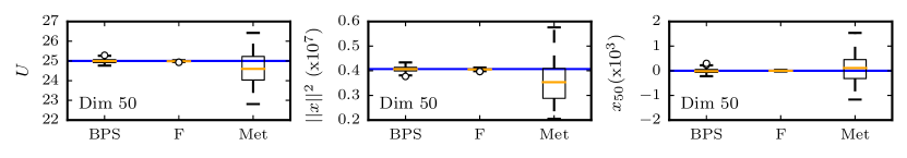
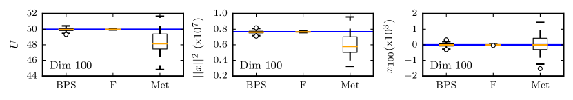
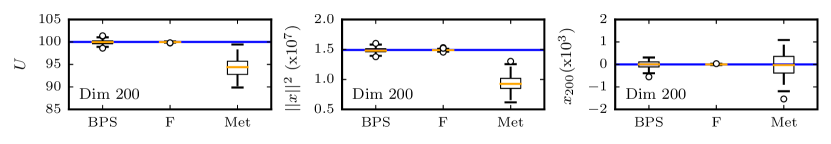
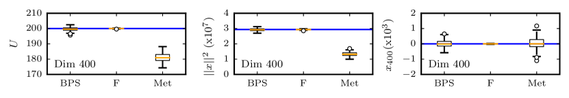
Figure 11: Box plots of $U$, $||x||^{2}$ and $x$ for the ill-conditioned zero-mean Gaussian distribution with covariance matrix given by (15) and $d=25,50,100,200$ and $400$. Each box represent the results of 100 runs of $10^{5}$ samples separated by a fixed CPU time $\sim 7.10^{-3}s$, resulting in $200$ updates for the Hastings-Metropolis (Met) algorithm and $\sim 55$ events for the BPS and Forward Ref (F).

D.2 Numerical comparisons between direct and Metropolis Forward event-chain methods

We compare the performances given by the choice of $K^{x,\sslash}$ between the direct, independent Metropolis and random-walk Metropolis ($\delta\in[-0.5,0.5]$) schemes, with a refreshment set to an orthogonal switch at fixed time $\mathrm{T}$ and $\bar{\lambda}=0$, corresponding to Algorithm 3.

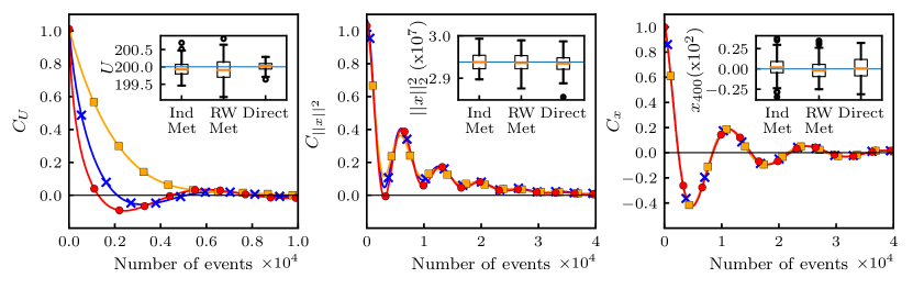
Figure 12: Autocorrelation functions $C$ of the potential $U$ (Left), $||x||^{2}$ (Middle) and $x$ (Right) for the ill-conditioned zero-mean Gaussian distribution with covariance matrix given by (15) and $d=400$ for Forward EC schemes with independent-Metropolis sampling (blue, crosses), random-walk Metropolis sampling (yellow, squares) and direct sampling (red, circles). Insets correspond to the respective boxplots for 100 runs of $10^{5}$ samples separated by a fixed time $T=500$ corresponding to an average of $55$ events.

For the anisotropic Gaussian distribution of Section 4.2, we set $\mathrm{T}=500$ ($\sim 55$ events in average). The autocorrelation functions for the potential $U$, the squared norm $\left\|x\right\|^{2}$ and $x$ are represented on Fig. 12 for $d=400$, as long as the respective boxplots. All schemes show similar decorrelation behavior for $x$, but for the potential and the norm, the sampling scheme mixing the less (random-Walk Metropolis) is the slowest and the sampling scheme mixing the most (direct) is the fastest. The direct sampling scheme is also more efficient regarding the norm.

For the mixture of Gaussian distributions considered in Section 4.4, Table 4 summarizes the ESS for $x$ and $\left\|x\right\|^{2}$ for $d=2,4$ and $5$. At very small dimension $d=2$, less-mixing schemes based on Metropolis updates appears to be slightly faster but quickly, as dimension increases, results are similar.

D.3 Numerical comparisons for different refreshment strategies for the direct Forward event-chain method

Fixing $K^{x,\sslash}$ to the direct-sampling kernel, we now compare different refreshment choices at fixed $\mathrm{T}$ for $K^{x,y_{\sslash},\perp}$ on the experiment with the anisotropic Gaussian distribution as described by (15), as illustrated by Fig. 13, where the autocorrelation functions for $U,||x||^{2}$ and $x$ are shown. Refreshment schemes are then separated into two groups depending on their action and the obtained decorrelation:

• the sparse-orthogonal group, where the refreshment only acts on a few orthogonal components, as

  • Orthogonal switch: two orthonormal vectors $e_{1},e_{2}$ of the orthogonal plane are defined by the Gram-Schmidt process and $y$ is transformed into $\tilde{y}=y+(\left\langle e_{2},y\right\rangle-\left\langle e_{1},y\right\rangle)(e_{1}-e_{2})$

  • Perpendicular orthogonal switch: same as above but $y$ is set to $\tilde{y}=y-\left\langle e_{1},y\right\rangle(e_{1}-e_{2})-\left\langle e_{2},y\right\rangle(e_{1}+e_{2})$.

  • ran-$2$-orthogonal: random rotation of $2$ orthogonal components defined by the Gram-Schmidt process.

• the global group, where all components can be resampled, as

  • Full-orthogonal refresh: full refreshment of the orthogonal components of the direction.

  • Full refresh: full refreshment of the direction.

More details on the definition of $K^{x,\sslash}$ can be found in Section 3.2.

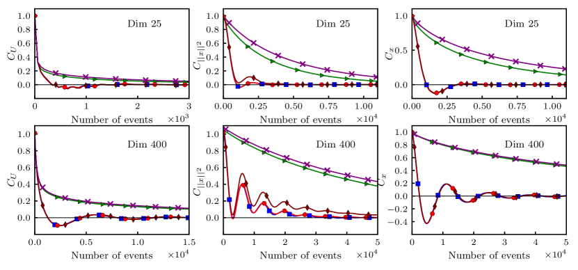
Figure 13: Autocorrelation functions $C$ of the potential $U$ (Left), the squared norm $||x||^{2}$ (Middle) and $x$ (Right) for the ill-conditioned zero-mean Gaussian distribution with covariance matrix given by (15) and $d=25$ (Top) and $d=400$ (Bottom) for direct Forward EC scheme with an orthogonal switch (red, circle), a perp orthogonal switch (maroon, slim diamond), a ran-$2$-p orthogonal switch (blue, square), a full orthogonal refresh (green, right triangle) and a full refresh (purple, cross). Every $K^{x,y_{\sslash},\perp}$ is set to its positive type.

For the small dimension ($d=25$) as the bigger one ($d=400$), a random-walk behavior appears in the global group, whereas in the sparse-orthogonal group, the antithetic correlations given by the ballistic trajectories are preserved and a faster decorrelation is achieved. In this group, the orthogonal switch scheme is the most efficient. In the global group, we observe that updating all the components but the one parallel to the gradient leads to a small acceleration in comparison to the standard full refreshment scheme. Finally, Figure 14 compares an orthogonal switch and a full-orthogonal refresh set at a fixed time $\mathrm{T}$ and at all event (no tuning of $\mathrm{T}$). It appears clearly that the orthogonal switch remains competitive without any tuning of $\mathrm{T}$, whereas the full-orthogonal refresh shows some convergence issue in that situation.

In Figure 13 and Figure 14, only positive-type $K^{x,y_{\sslash},\perp}$ are exhibited. Figure 15 compares positive to naive schemes and shows that the positive schemes are slightly better for the sampling of the anisotropic distribution.

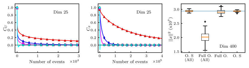
Figure 14: Autocorrelation functions $C$ of the potential $U$ (Left) and $x$ (Middle) for $d=25$ and box plots for $\left\|x\right\|^{2}$ (Right) for $d=400$ for the ill-conditioned $d-$dimensional zero-mean Gaussian distribution with covariance matrix given by (15) for direct Forward EC scheme to an orthogonal switch (O. S.) at fixed time (cyan, circle) and at all events (blue, diamond) and a full-orthogonal refresh (Full O.) at fixed time (magenta, square) and at all events (red, diamond). Every $K^{x,y_{\sslash},\perp}$ is set to its positive type. Box plots are based on $100$ runs of $10^{5}$ samples separated by $\mathrm{T}=500$.

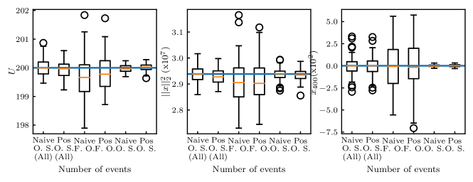
Figure 15: Box plots of $U$, $||x||^{2}$ and $x$ for the ill-conditioned zero-mean Gaussian distribution with covariance matrix given by (15) and $d=400$. Each box represent the results of 100 runs of $10^{5}$ samples separated by a fixed time $\mathrm{T}=500$ ($\sim 55$ events). Pos stands for Positive, Orth S. for orthogonal switch and F. O. for full-orthogonal refresh.

Finally, we show in Figure 16 the performance of BPS with different refreshment schemes, as to check whether accelerations can be achieved only by a choice of $K^{x,y_{\sslash},\perp}$ different from $\operatorname{Id}$, while still keeping $K^{x,\sslash}$ set to the deterministic choice of the reflection. We consider the standard Full Ref in a naive and positive implementation and a orthogonal switch at fixed time $\mathrm{T}$ associated with $\bar{\lambda}=0$, also in a positive and naive settings. Positive and naive types give similar results. However, it appears clearly that BPS set to the sparse-orthogonal refreshment scheme of the orthogonal switch is not able to recover a correct estimate of the potential $U$, while the decorrelation in respect of $x$ is fast. BPS requires indeed a strong refreshment as the deterministic choice of $K^{x,\sslash}$ leads to poor mixing for $U$, but at the cost of a slow decay of $x$.

Figure 16: Box plots of $U$ and $||x||^{2}$ for the ill-conditioned zero-mean Gaussian distribution with covariance matrix given by (15) and $d=400$. Each box represent the results of 100 runs of $10^{5}$ samples separated by a fixed time $\mathrm{T}=500$ ($\sim 55$ events). Pos stands for Positive, Orth S. for orthogonal switch and Full for Full Ref.

D.4 Impact of the choice of the refreshment parameters

We consider the zero-mean Gaussian distribution with covariance matrix given by (15) and study the effects of the refreshment time $\mathrm{T}$ tuning on the integrated autocorrelation times for the Forward Ref (see Figure 17), Forward Full Ref (see Figure 18), BPS Full Ref (see Figure 19) and Forward Ref set to a full-orthogonal refreshment (see Figure 20).

Figure 17: Integrated autocorrelation times $\tau$ of $U$ (Left), $\left\|x\right\|^{2}$ (Middle) and $x$ (Right) for the anisotropic Gaussian distribution for Forward Ref for different refreshment time $\mathrm{T}$ ($\mathrm{T}=0$ corresponds to Forward Ref All). Error bars may be covered by the markers.

Figure 18: Integrated autocorrelation times $\tau$ of $U$ (Left), $\left\|x\right\|^{2}$ (Middle) and $x$ (Right) for the anisotropic Gaussian distribution for Forward Full Ref for different refreshment time $\mathrm{T}$. Error bars may be covered by the markers.

Figure 19: Integrated autocorrelation times $\tau$ of $U$ (Left), $\left\|x\right\|^{2}$ (Middle) and $x$ (Right) for the anisotropic Gaussian distribution for BPS Full Ref for different refreshment time $\mathrm{T}$. Error bars may be covered by the markers.

Figure 20: Integrated autocorrelation times $\tau$ of $U$ (Left), $\left\|x\right\|^{2}$ (Middle) and $x$ (Right) for the anisotropic Gaussian distribution for direct Forward EC set to full-orthogonal refresh for different refreshment time $\mathrm{T}$. Error bars may be covered by the markers.

Figure 21: Integrated autocorrelation times $\tau$ of $U$ (Left), $\left\|x\right\|^{2}$ (Middle) and $x$ (Right) for the anisotropic Gaussian distribution for direct Forward EC set to ran-p-orthogonal refresh for different value of $p$. Error bars may be covered by the markers.

Figure 22: Integrated autocorrelation times $\tau$ of $U$ (Left), $\left\|x\right\|^{2}$ (Middle) and $x$ (Right) for the anisotropic Gaussian distribution for direct Forward EC set to $2$-orthogonal refresh for different value of $\theta$ and $\mathrm{T}=0$ (crosses) and $\mathrm{T}=500$ (circles). Error bars may be covered by the markers.

A first observation is that the scaling with the dimension of the integrated autocorrelation time of $x$ is similar for any choice of $\mathrm{T}$ and the offset decreases as $\mathrm{T}$ increases (less randomization), for all schemes. For the potential $U$ and the squared norm $\left\|x\right\|^{2}$, on the contrary, there is a trade-off to find between controlling the random-walk behavior and trapping the process into a loop. Forward Ref appears as the most robust concerning this tuning, as all choices of $\mathrm{T}$ are in the same range. BPS Full Ref, on the opposite, needs $\mathrm{T}$ small enough to decorrelate the potential $U$, at the cost of the norm decorrelation. Comparing it to the results for Forward Full Ref, we can observe that the direct-sampling scheme helps with the decorrelation of $U$ and allows to set $\mathrm{T}$ to very high values. The choice $\mathrm{T}=10^{4}$ appears as an optimal, leading to a maximal integrated time of order $2\times 10^{3}$, which is competitive with Forward Ref. However, Forward Full Ref is more sensitive to the tuning of $\mathrm{T}$ than Forward Ref. Same behavior can be observed for Forward Ref with full-orthogonal refreshment, as displayed in Figure 20.

We show in Figure 21 and Figure 22 the dependence of the integrated autocorrelation times with respectively $p$ in Forward Ref with a ran-$p$-orthogonal refreshment and with $\theta$ in Forward Ref and Forward All Ref with a $2$-orthogonal refreshment. The choice of $p$ appears not to be critical and Figure 22 shows a non-dependence on the angle $\theta$.

D.5 ESS for mixture of Gaussian distributions

We consider the mixture of five Gaussian distributions of Section 4.4. For small dimensions $d=2,4,5$, the estimated ESS are similar for all considered schemes, as can be observed in Table 4.

Table 4: ESS per event for the mixture of five Gaussian distributions.

d	h	DF. No Ref	DF. Ref	DF. Ref All	DF. Full Ref	BPS No Ref	BPS Full Ref	IMF No Ref	IMF Ref	RWMF No Ref	RWMF Ref
$2$	$x$	1453$\pm$27	–	–	1364$\pm$2	1729$\pm$34	1608$\pm$30	1535$\pm$24	–	1660$\pm$25	–
$2$	$\left\|x\right\|^{2}$	1501$\pm$27	–	–	1403$\pm$22	1726$\pm$35	1621$\pm$32	1578$\pm$25	–	1696$\pm$25	–
$4$	$x$	54$\pm$5	59$\pm$4	53$\pm$4	55$\pm$4	58$\pm$4	59$\pm$4	62$\pm$5	62$\pm$4	58$\pm$6	59$\pm$6
$4$	$\left\|x\right\|^{2}$	63$\pm$5	69$\pm$5	60$\pm$5	64$\pm$4	67$\pm$5	68$\pm$4	72$\pm$6	72$\pm$5	67$\pm$6	67$\pm$8
$5$	$x$	26$\pm$3	25$\pm$3	23$\pm$5	25$\pm$3	24$\pm$4	26$\pm$3	27$\pm$3	28$\pm$3	26$\pm$3	25$\pm$3
$5$	$\left\|x\right\|^{2}$	33$\pm$4	32$\pm$3	28$\pm$4	31$\pm$4	31$\pm$5	33$\pm$4	35$\pm$4	35$\pm$3	32$\pm$3	31$\pm$3

NOTE: Results are multiplied by $10^{5}$. For $d=2$, there is no orthogonal refreshment. DF.: Direct Forward. IMF: independent-Metropolis Forward. RWMF: random-walk Metropolis Forward.

References

- Andrieu and Livingstone (2019) Andrieu, C. and S. Livingstone (2019). Peskun-tierney ordering for markov chain and process monte carlo: beyond the reversible scenario. arXiv preprint arXiv:1906.06197.
- Bernard and Krauth (2011) Bernard, E. P. and W. Krauth (2011). Two-step melting in two dimensions: First-order liquid-hexatic transition. Phys. Rev. Lett. 107, 155704.
- Bernard et al. (2009) Bernard, E. P., W. Krauth, and D. B. Wilson (2009). Event-Chain Monte Carlo algorithms for hard-sphere systems. Physical Review E 80, 056704.
- Beskos et al. (2013) Beskos, A., N. Pillai, G. Roberts, J.-M. Sanz-Serna, and A. Stuart (2013, 11). Optimal tuning of the hybrid monte carlo algorithm. Bernoulli 19(5A), 1501–1534.
- Bierkens et al. (2019) Bierkens, J., P. Fearnhead, and G. Roberts (2019). The Zig-Zag process and super-efficient sampling for Bayesian analysis of big data. Ann. Statist. 47(3), 1288–1320.
- Bierkens and Roberts (2017) Bierkens, J. and G. Roberts (2017). A piecewise deterministic scaling limit of lifted Metropolis-Hastings in the Curie-Weiss model. Ann. Appl. Probab. 27(2), 846–882.
- Bierkens et al. (2019) Bierkens, J., G. Roberts, and P.-A. Zitt (2019). Ergodicity of the Zig-Zag process. Ann. Appl. Probab. 29(4), 2266–2301.
- Bouchard-Côté et al. (2018) Bouchard-Côté, A., S. J. Vollmer, and A. Doucet (2018). The bouncy particle sampler. JASA 113(522), 855–867.
- Carpenter et al. (2017) Carpenter, B., A. Gelman, M. Hoffman, D. Lee, B. Goodrich, M. Betancourt, M. Brubaker, J. Guo, P. Li, and A. Riddell (2017). Stan: A probabilistic programming language. Journal of Statistical Software, Articles 76(1), 1–32.
- Chen et al. (1999) Chen, F., L. Lovász, and I. Pak (1999). Lifting Markov chains to speed up mixing. In Proc. of ACM STOC, pp. 275–281.
- Davis (1993) Davis, M. (1993). Markov Models & Optimization, Volume 49. CRC Press.
- Diaconis et al. (2000) Diaconis, P., S. Holmes, and R. M. Neal (2000). Analysis of a nonreversible Markov chain sampler. Ann. Appl. Probab. 10(3), 726–752.
- Dua and Efi (2017) Dua, D. and K. Efi (2017). UCI machine learning repository.
- Duane et al. (1987) Duane, S., A. D. Kennedy, B. J. Pendelton, and D. Roweth (1987). Hybrid Monte Carlo. Physics Letters B 195, 216–222.
- Gelfand and Smith (1990a) Gelfand, A. E. and A. F. Smith (1990a). Sampling-based approaches to calculating marginal densities. Journal of the American statistical association 85(410), 398–409.
- Gelfand and Smith (1990b) Gelfand, A. E. and A. F. M. Smith (1990b). Sampling-based approaches to calculating marginal densities. Journal of the American Statistical Association 85, 398–409.
- Geman and Geman (1984) Geman, S. and D. Geman (1984). Stochastic relaxation, Gibbs distributions and the Bayesian restoration of images. IEEE Transactions on Pattern Analysis and Machine Intelligence 6, 721–741.
- Girolami and Calderhead (2011) Girolami, M. and B. Calderhead (2011). Riemann manifold Langevin and Hamiltonian Monte Carlo methods. Journal of the Royal Statistical Society Series B 73, Part 2, 123–214.
- Harland et al. (2017) Harland, J., M. Michel, T. A. Kampmann, and J. Kierfeld (2017). Event-Chain Monte Carlo algorithms for three- and many-particle interactions. EPL 117(3), 30001.
- Hastings (1970) Hastings, W. K. (1970). Monte Carlo sampling methods using Markov chains and their applications. Biometrika 57, 97–109.
- Hoffman and Gelman (2014) Hoffman, M. D. and A. Gelman (2014). The No-U-Turn Sampler: adaptively setting path lengths in Hamiltonian Monte Carlo. Journal of Machine Learning Research 2014(15), 1593–1623.
- Kapfer and Krauth (2015) Kapfer, S. C. and W. Krauth (2015). Two-dimensional melting: From liquid-hexatic coexistence to continuous transitions. Physical Review Letters 114, 035702.
- Metropolis et al. (1953) Metropolis, M., A. W. Rosenbluth, M. N. Rosenbluth, A. H. Teller, and E. Teller (1953). Equation of state calculation by fast computing machines. Journal of Chemical Physics 21, 1087–1092.
- Michel (2016) Michel, M. (2016, October). Irreversible Markov chains by the factorized Metropolis filter : algorithms and applications in particle systems and spin models. Phd thesis, École Normale Supérieure de Paris.
- Michel et al. (2014) Michel, M., S. C. Kapfer, and W. Krauth (2014). Generalized Event-Chain Monte Carlo: Constructing rejection-free global-balance algorithms from infinitesimal steps. The Journal of chemical physics 140(5), 054116.
- Michel et al. (2019) Michel, M., X. Tan, and Y. Deng (2019). Clock monte carlo methods. Physical Review E 99, 010105(R).
- Monmarché (2016) Monmarché, P. (2016). Piecewise deterministic simulated annealing. ALEA Lat. Am. J. Probab. Math. Stat. 13(1), 357–398.
- Neal (1996) Neal, R. M. (1996). Bayesian Learning for Neural Networks. Lecture Notes in Statistics 118, Springer.
- Neal (2004) Neal, R. M. (2004). Improving asymptotic variance of MCMC estimators: Non-reversible chains are better. Technical Report Technical Report No. 0406, Dept. of Statistics, University of Toronto.
- Nishikawa et al. (2015) Nishikawa, Y., M. Michel, W. Krauth, and K. Hukushima (2015). Event-Chain algorithm for the heisenberg model: Evidence for z 1 dynamic scaling. Physical Review E 92, 063306.
- Peters and de With (2012) Peters, E. A. J. F. and G. de With (2012). Rejection-free Monte Carlo sampling for general potentials. Phys. Rev. E 85, 026703.
- Robert and Casella (1999) Robert, C. P. and G. Casella (1999). Monte Carlo Statistical Methods. Springer Texts in Statistics. Springer.
- Sakai and Hukushima (2013) Sakai, Y. and K. Hukushima (2013). Dynamics of one-dimensional ising model without detailed balance condition. Journal of the Physical Society of Japan 82(6), 064003.
- Sohl-Dickstein et al. (2014) Sohl-Dickstein, J., M. Mudigonda, and M. R. DeWeese (2014). Hamiltonian Monte Carlo without detailed balance. In J. W. volume 32 (Ed.), Proc. ICML.
- Vanetti et al. (2017) Vanetti, P., A. Bouchard-Côté, G. Deligiannidis, and A. Doucet (2017). Piecewise Deterministic Markov Chain Monte Carlo. arXiv preprint arXiv:1707.05296.
- Wang et al. (2013) Wang, Z., S. Mohamed, and N. de Freitas (2013). Adaptive Hamiltonian and Riemann manifold Monte Carlo samplers. In J. W. volume 28 (Ed.), Proc. ICML.
- Wu and Robert (2017) Wu, C. and C. P. Robert (2017). Generalized Bouncy Particle Sampler. arXiv preprint arXiv:1706.04781.

References

- Bernard et al. (2009) Bernard, E. P., W. Krauth, and D. B. Wilson (2009). Event-Chain Monte Carlo algorithms for hard-sphere systems. Physical Review E 80, 056704.
- Bogachev (2006) Bogachev, V. (2006). Measure Theory. Springer Berlin Heidelberg.
- Bouchard-Côté et al. (2018) Bouchard-Côté, A., S. J. Vollmer, and A. Doucet (2018). The bouncy particle sampler. JASA 113(522), 855–867.
- Davis (1993) Davis, M. (1993). Markov Models & Optimization, Volume 49. CRC Press.
- Ethier and Kurtz (1986) Ethier, S. N. and T. G. Kurtz (1986). Markov processes. Wiley Series in Probability and Mathematical Statistics: Probability and Mathematical Statistics. New York: John Wiley & Sons Inc. Characterization and convergence.
- Michel et al. (2014) Michel, M., S. C. Kapfer, and W. Krauth (2014). Generalized Event-Chain Monte Carlo: Constructing rejection-free global-balance algorithms from infinitesimal steps. The Journal of chemical physics 140(5), 054116.
- Michel et al. (2019) Michel, M., X. Tan, and Y. Deng (2019). Clock monte carlo methods. Physical Review E 99, 010105(R).
- Peters and de With (2012) Peters, E. A. J. F. and G. de With (2012). Rejection-free Monte Carlo sampling for general potentials. Phys. Rev. E 85, 026703.