Amplitude reconstruction from complete electroproduction experiments and truncated partial-wave expansions

Abstract

We compare the methods of amplitude reconstruction, for a complete experiment and a truncated partial-wave analysis, applied to the electroproduction of pseudoscalar mesons. We give examples which show, in detail, how the amplitude reconstruction (observables measured at a single energy and angle) is related to a truncated partial-wave analysis (observables measured at a single energy and a number of angles). A connection is made to existing data.

I Introduction and Motivation

There have been numerous recent efforts to extract maximal information, unbiased by any particular model, from experimental pseudoscalar photoproduction data. These have included the study of complete experiment analyses CEA (CEA) and truncated partial-wave analyses TPWA (TPWA). Legendre analyses directly applied to data Leg have the same motivation. The CEA determines helicity or transversity amplitudes at a single energy and angle, up to an overall (energy and angle dependent) phase. The TPWA introduces a cutoff to the partial-wave series, obtaining multipoles for a fixed energy, with an overall unknown phase dependent only on energy.

The methods used to study the photoproduction of pseudoscalar mesons can be extended to the case of electroproduction, with the introduction of longitudinal amplitudes associated with the incoming virtual photon. An examination of the CEA was performed by Dmitrasinovic, Donnelly and Gross DDG who considered the required polarization measurements. They concluded that a CEA, determining the electroproduction transversity amplitudes up to an overall phase, was not possible with either recoil or target polarization measurements alone, but required at least one measurement from the other polarization set. They further concluded that a CEA could be constructed without the need for more complicated measurements involving both a polarized target and recoil polarization detection. These conclusions assumed that all structure functions could be separated in a set of measurements. As in all such studies, it was also implicitly assumed that measurements could be made arbitrarily precise.

Here we generalize our recent study TPWA of the CEA and TPWA in photoproduction to electroproduction. While the study in Ref. DDG focused on the CEA, in practice, one desires multipole amplitudes that can be associated with resonance contributions. These cannot be directly obtained from a complete set of transversity amplitudes and the methods used in solving the CEA and TPWA problems are quite different, as was discussed in detail in Ref. TPWA .

The electroproduction reaction, unlike photoproduction, requires detailed knowledge of the electron scattering process producing the interacting virtual photon. As the electron scattering and outgoing hadronic particles define two different planes, a second angle defining their relative orientation is required, as shown in Fig. 1. The virtual photon can have a non-zero value for its 4-momentum squared, which allows for the independent variation of photon energy and momentum.

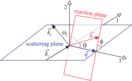
Figure 1: Kinematics of an electroproduction experiment. The scattering plane {1,3} is defined by the respective incoming and outgoing electron momenta $\vec{k}_{i}$, $\vec{k}_{f}$ with the electron scattering angle $\Theta_{e}$. The reaction plane is spanned by the virtual photon $\vec{q}$ and the outgoing meson $\vec{k}$, scattered by the angle $\theta$. The reaction plane is tilted versus the scattering plane by the azimuthal angle $\phi$.

This non-zero value also complicates the spin structure, requiring the introduction of both longitudinal and transverse components, as described in Refs. Drechsel:1992pn ; Knochlein:1995qz . Below, we first review the electroproduction formalism. We then consider both simple and more realistic examples of the CEA and TPWA process, showing how the experimental requirements change.

II Cross Section and Polarization Degrees of Freedom

Here we follow the notation of Ref. Knochlein:1995qz to describe the pseudoscalar meson electroproduction process. As denoted in Fig. 1, $\Theta_{e}$ is the electron scattering angle while $q$ and $k$ are the respective 4-vectors for the virtual photon and outgoing meson, with $q^{2}=\omega^{2}-\mathbb{q}^{2}$, $\omega$ and $\mathbb{q}$ being the photon energy and 3-momentum. The momentum transfer is denoted by $Q^{2}=-q^{2}$ and the “photon equivalent energy” is given by $k_{\gamma}^{lab}=(W^{2}-m_{i}^{2})/2m_{i}$, where $W$ is the center-of-mass energy of the hadronic system and $m_{i}$ is the mass of the initial nucleon. The degree of transverse polarization of the virtual photon is

$$\varepsilon=\left(1+{2\mathbb{q}^{2}\over{Q^{2}}}\tan^{2}{\Theta_{e}\over 2}\right)^{-1}\,,$$ (1)

with $\mathbb{q}$ and $\Theta_{e}$ expressible in either the lab or c.m. frame. The longitudinal polarization,

$$\varepsilon_{L}={Q^{2}\over{\omega^{2}}}\,\varepsilon\,,$$ (2)

is frame dependent.

Experiments with three types of polarization can be performed in meson electroproduction: electron beam polarization, polarization of the target nucleon and polarization of the recoil nucleon. Target polarization will be described in the frame $\{x,y,z\}$, with the $z$-axis pointing in the direction of the photon momentum $\hat{\mathbb{q}}$, the $y$-axis perpendicular to the reaction plane, $\hat{\mathbb{y}}=\hat{\mathbb{q}}\times\hat{\mathbb{k}}/\sin\theta$, where $\hat{\mathbb{k}}$ is the direction of the outgoing meson, and the $x$-axis given by $\hat{\mathbb{x}}=\hat{\mathbb{y}}\times\hat{\mathbb{z}}$. For recoil polarization we will use the frame $\{x^{\prime},y^{\prime},z^{\prime}\}$, with the $z^{\prime}$-axis defined by the momentum vector of the outgoing meson, the $y^{\prime}$-axis parallel to $\hat{\mathbb{y}}$, and the $x^{\prime}$-axis given by $\hat{\mathbb{x}}^{\prime}=\hat{\mathbb{y}}^{\prime}\times\hat{\mathbb{z}}^{\prime}$. These frames are displayed in Fig. 2.

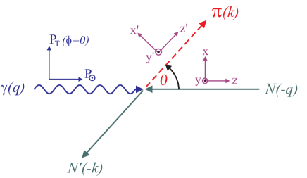
Figure 2: Frames for polarization vectors. Target and recoil polarization are commonly defined as $\{x,y,z\}$ and $\{x^{\prime},y^{\prime},z^{\prime}\}$ in the c.m. frame, with the $z^{\prime}$ direction along the outgoing meson $\pi(k)$. The virtual photon $\gamma(q)$ can carry different types of polarization, including the linear and circular polarizations, $P_{T}$ in the $\{x,y\}$ plane and $P_{\odot}$ along the $z$ axis, as in photoproduction. In addition, the longitudinal photon carries a polarization, $\varepsilon_{L}$, with further polarization types appearing in the $LT$ interferences of Eq. (II).

The most general expression for a coincidence experiment considering all three types of polarization is

$$\frac{d\sigma_{v}}{d\Omega} =\frac{|\vec{k}|}{k_{\gamma}^{cm}}P_{\alpha}P_{\beta}\Big{\{}R_{T}^{\beta\alpha}+\varepsilon_{L}R_{L}^{\beta\alpha}$$

$$\quad\mbox{}+\left[2\varepsilon_{L}\left(1+\varepsilon\right)\right]^{1/2}(^{c}\!R_{LT}^{\beta\alpha}\cos\phi+^{s}\!\!R_{LT}^{\beta\alpha}\sin\phi)$$

$$\quad\mbox{}+\varepsilon(^{c}\!R_{TT}^{\beta\alpha}\cos 2\phi+^{s}\!R_{TT}^{\beta\alpha}\sin 2\phi)$$

$$\quad\mbox{}+h\left[2\varepsilon_{L}(1-\varepsilon)\right]^{1/2}(^{c}\!R_{LT^{\prime}}^{\beta\alpha}\cos\phi+^{s}\!R_{LT^{\prime}}^{\beta\alpha}\sin\phi)$$

$$\quad\mbox{}+h(1-\varepsilon^{2})^{1/2}R_{TT^{\prime}}^{\beta\alpha}\Big{\}}\,,$$ (3)

where $h$ is the helicity of the incoming electron, $P_{\alpha}=(1,\vec{P})_{\alpha}$ and $P_{\beta}=(1,\vec{P}^{\prime})_{\beta}$. Here $\vec{P}=(P_{x},P_{y},P_{z})$ denotes the target and $\vec{P}^{\prime}=(P_{x^{\prime}},P_{y^{\prime}},P_{z^{\prime}})$ the recoil polarization vector. The zero components, $P_{0}=1$, lead to contributions in the cross section which are present in the polarized as well as the unpolarized case. In an experiment without target and recoil polarization, $\alpha=\beta=0$ and the only remaining contributions are $R_{i}^{00}$. The functions $R_{i}^{\beta\alpha}$ describe the response of the hadronic system in the process. Summation over Greek indices (0,1,2,3) is implied. An additional superscript $s$ or $c$ on the left indicates a sine or cosine dependence of the respective contribution on the azimuthal angle. Some response functions vanish identically (see Table 1 of Ref. Knochlein:1995qz for a systematic overview). The number of different response functions is further reduced by equalities, as shown in Table 1, and in the most general electroproduction experiment, 36 polarization observables can be determined. The response functions $R^{\beta\alpha}_{i}$ are real or imaginary parts of bilinear forms of the CGLN CGLN amplitudes depending on the scattering angle $\theta$.

III Amplitudes used in pseudoscalar meson electroproduction

Before comparing the CEA and TPWA approaches, we continue with a review of notation used for the underlying amplitudes. The multipoles and CGLN CGLN $F$-amplitudes are related by

$$F_{1} =\sum_{\ell\geq 0}\left[\left(\ell M_{\ell+}+E_{\ell+}\right)P^{\prime}_{\ell+1}+\left((\ell+1)M_{\ell-}+E_{\ell-}\right)P^{\prime}_{\ell-1}\right]\,,$$ (4a)

$$F_{2} =\sum_{\ell\geq 1}\left[(\ell+1)M_{\ell+}+\ell M_{\ell-}\right]P^{\prime}_{\ell}\,,$$ (4b)

$$F_{3} =\sum_{\ell\geq 1}\left[\left(E_{\ell+}-M_{\ell+}\right)P^{\prime\prime}_{\ell+1}+\left(E_{\ell-}+M_{\ell-}\right)P^{\prime\prime}_{\ell-1}\right]\,,$$ (4c)

$$F_{4} =\sum_{\ell\geq 2}\left[M_{\ell+}-E_{\ell+}-M_{\ell-}-E_{\ell-}\right]P^{\prime\prime}_{\ell}\,,$$ (4d)

$$F_{5} =\sum_{\ell\geq 0}\left[(\ell+1)L_{\ell+}P^{\prime}_{\ell+1}-\ell\;L_{\ell-}P^{\prime}_{\ell-1}\right]\,,$$ (4e)

$$F_{6} =\sum_{\ell\geq 1}\left[\ell\;L_{\ell-}-(\ell+1)L_{\ell+}\right]P^{\prime}_{\ell}\,.$$ (4f)

The definition of helicity amplitudes is subject to phase conventions. Here, we choose the conventions of Jacob , which were also used by Walker in Walker for photoproduction. Without loss of generality, we set $\phi=0$,

$$H_{1} =-\frac{1}{\sqrt{2}}\sin\theta\cos\frac{\theta}{2}(F_{3}+F_{4})\,,$$ (5a)

$$H_{2} =\sqrt{2}\cos\frac{\theta}{2}\left(F_{2}-F_{1}+(F_{3}-F_{4})\sin^{2}\frac{\theta}{2}\right)\,,$$ (5b)

$$H_{3} =\frac{1}{\sqrt{2}}\sin\theta\sin\frac{\theta}{2}(F_{3}-F_{4})\,,$$ (5c)

$$H_{4} =\sqrt{2}\sin\frac{\theta}{2}\left(F_{1}+F_{2}+(F_{3}+F_{4})\cos^{2}\frac{\theta}{2}\right)\,,$$ (5d)

$$H_{5} =\cos\frac{\theta}{2}(F_{5}+F_{6})\,,$$ (5e)

$$H_{6} =-\sin\frac{\theta}{2}(F_{5}-F_{6})\,.$$ (5f)

Finally, transversity amplitudes can be constructed bds ; DDG from these helicity amplitudes,

$$b_{1} =\frac{1}{2}\left[\left(H_{1}+H_{4}\right)\;+\;i\;\left(H_{2}-H_{3}\right)\right]\,,$$ (6a)

$$b_{2} =\frac{1}{2}\left[\left(H_{1}+H_{4}\right)\;-\;i\;\left(H_{2}-H_{3}\right)\right]\,,$$ (6b)

$$b_{3} =\frac{1}{2}\left[\left(H_{1}-H_{4}\right)\;-\;i\;\left(H_{2}+H_{3}\right)\right]\,,$$ (6c)

$$b_{4} =\frac{1}{2}\left[\left(H_{1}-H_{4}\right)\;+\;i\;\left(H_{2}+H_{3}\right)\right]\,,$$ (6d)

$$b_{5} =\frac{1}{\sqrt{2}}\left[H_{5}\;+\;i\;H_{6}\right]\,,$$ (6e)

$$b_{6} =\frac{1}{\sqrt{2}}\left[H_{5}\;-\;i\;H_{6}\right]\,.$$ (6f)

Here we note that the definitions of both helicity and transversity amplitudes are not unique. Apart from phase conventions, different numbering choices can also be found in the literature. Here we follow the definitions of Barker et al. bds . In Table 1, expressions for the response functions, appearing in Eq. (II), are given in terms of both the helicity and transversity amplitudes. In the following, we will suppress the superscripts $c$ and $s$ for interference terms. As can be seen in Table 1, for a specific polarization, the assignment of this superscript is always unique.

Table 1: Spin observables expressed in terms of helicity and transversity amplitudes. Also listed are alternate (ALT) observables, differing by at most a sign in their definition, and associated photoproduction observables ($\gamma$). Note, that these expressions are not uniquely defined. We follow the conventions of Refs. bds ; Walker .

Obs	ALT	$\gamma$	Helicity	Transversity
			representation	representation
$R_{T}^{00}$	$-^{c}\!R_{TT}^{y^{\prime}y}$	$I$	$\frac{1}{2}$ ($|H_{1}|^{2}+|H_{2}|^{2}+|H_{3}|^{2}+|H_{4}|^{2}$)	$\frac{1}{2}(|b_{1}|^{2}+|b_{2}|^{2}+|b_{3}|^{2}+|b_{4}|^{2}$)
$R_{T}^{0y}$	$-^{c}\!R_{TT}^{y^{\prime}0}$	$\check{T}$	$-$Im$(H_{2}H_{1}^{*}+H_{4}H_{3}^{*})$	$\frac{1}{2}(|b_{1}|^{2}-|b_{2}|^{2}-|b_{3}|^{2}+|b_{4}|^{2})$
$R_{T}^{y^{\prime}0}$	$-^{c}\!R_{TT}^{0y}$	$\check{P}$	Im$(H_{3}H_{1}^{*}+H_{4}H_{2}^{*})$	$\frac{1}{2}(|b_{1}|^{2}-|b_{2}|^{2}+|b_{3}|^{2}-|b_{4}|^{2}$)
$R_{T}^{x^{\prime}x}$	$-^{c}\!R_{TT}^{z^{\prime}z}$	$\check{T}_{x^{\prime}}$	Re$(H_{4}H_{1}^{*}+H_{3}H_{2}^{*})$	Re($b_{1}b_{2}^{*}-b_{4}b_{3}^{*}$)
$R_{T}^{x^{\prime}z}$	${}^{c}\!R_{TT}^{z^{\prime}x}$	$-\check{L}_{x^{\prime}}$	Re$(H_{3}H_{1}^{*}-H_{4}H_{2}^{*})$	${\rm Im}(b_{4}b_{3}^{*}-b_{1}b_{2}^{*})$
$R_{T}^{z^{\prime}x}$	${}^{c}\!R_{TT}^{x^{\prime}z}$	$\check{T}_{z^{\prime}}$	Re$(H_{2}H_{1}^{*}-H_{4}H_{3}^{*})$	${\rm Im}(b_{1}b_{2}^{*}+b_{4}b_{3}^{*})$
$R_{T}^{z^{\prime}z}$	$-^{c}\!R_{TT}^{x^{\prime}x}$	$\check{L}_{z^{\prime}}$	$\frac{1}{2}(|H_{1}|^{2}-|H_{2}|^{2}-|H_{3}|^{2}+|H_{4}|^{2})$	${\rm Re}(b_{1}b_{2}^{*}+b_{4}b_{3}^{*})$
$R_{L}^{00}$	$-R_{L}^{y^{\prime}y}$		$|H_{5}|^{2}+|H_{6}|^{2}$	$|b_{5}|^{2}+|b_{6}|^{2}$
$R_{L}^{0y}$	$-R_{L}^{y^{\prime}0}$		$-2{\rm Im}(H_{6}H_{5}^{*})$	$|b_{5}|^{2}-|b_{6}|^{2}$
$R_{L}^{x^{\prime}x}$	$-R_{L}^{z^{\prime}z}$		$-|H_{5}|^{2}+|H_{6}|^{2}$	$-2{\rm Re}(b_{6}b_{5}^{*})$
$R_{L}^{z^{\prime}x}$	$R_{L}^{x^{\prime}z}$		$2{\rm Re}(H_{6}H_{5}^{*})$	$-2{\rm Im}(b_{6}b_{5}^{*})$
${}^{c}\!R_{LT}^{00}$	$-^{c}\!R_{LT}^{y^{\prime}y}$		$\frac{1}{\sqrt{2}}{\rm Re}\left((H_{1}-H_{4})H_{5}^{*}+(H_{2}+H_{3})H_{6}^{*}\right)$	${\rm Re}(b_{6}b_{3}^{*}+b_{5}b_{4}^{*})$
${}^{s}\!R_{LT}^{0x}$	${}^{c}\!R_{LT^{\prime}}^{y^{\prime}z}$		$\frac{1}{\sqrt{2}}{\rm Im}((H_{3}-H_{2})H_{5}^{*}-(H_{1}+H_{4})H_{6}^{*})$	${\rm Re}(b_{1}b_{6}^{*}-b_{5}b_{2}^{*})$
${}^{c}\!R_{LT}^{0y}$	$-^{c}\!R_{LT}^{y^{\prime}0}$		$-\frac{1}{\sqrt{2}}{\rm Im}((H_{2}+H_{3})H_{5}^{*}-(H_{1}-H_{4})H_{6}^{*})$	${\rm Re}(b_{5}b_{4}^{*}-b_{6}b_{3}^{*})$
${}^{s}\!R_{LT}^{0z}$	$-^{c}\!R_{LT^{\prime}}^{y^{\prime}x}$		$-\frac{1}{\sqrt{2}}{\rm Im}((H_{1}+H_{4})H_{5}^{*}-(H_{2}-H_{3})H_{6}^{*})$	${\rm Im}(b_{5}b_{2}^{*}-b_{1}b_{6}^{*})$
${}^{s}\!R_{LT}^{x^{\prime}0}$	$-^{c}\!R_{LT^{\prime}}^{z^{\prime}y}$		$\frac{1}{\sqrt{2}}{\rm Im}((H_{2}-H_{3})H_{5}^{*}-(H_{1}+H_{4})H_{6}^{*})$	${\rm Re}(b_{6}b_{2}^{*}-b_{1}b_{5}^{*})$
${}^{s}\!R_{LT}^{z^{\prime}0}$	${}^{c}\!R_{LT^{\prime}}^{x^{\prime}y}$		$-\frac{1}{\sqrt{2}}{\rm Im}((H_{1}+H_{4})H_{5}^{*}+(H_{2}-H_{3})H_{6}^{*})$	${\rm Im}(b_{6}b_{2}^{*}-b_{1}b_{5}^{*})$
${}^{c}\!R_{LT}^{x^{\prime}x}$	$-^{c}\!R_{LT}^{z^{\prime}z}$		$-\frac{1}{\sqrt{2}}{\rm Re}((H_{1}-H_{4})H_{5}^{*}-(H_{2}+H_{3})H_{6}^{*})$	$-{\rm Re}(b_{5}b_{3}^{*}+b_{6}b_{4}^{*})$
${}^{c}\!R_{LT}^{z^{\prime}x}$	${}^{c}\!R_{LT}^{x^{\prime}z}$		$\frac{1}{\sqrt{2}}{\rm Re}((H_{2}+H_{3})H_{5}^{*}+(H_{1}-H_{4})H_{6}^{*})$	${\rm Im}(b_{5}b_{3}^{*}-b_{6}b_{4}^{*})$

Table 1: (continued)

Obs	ALT	$\gamma$	Helicity	Transversity
			representation	representation
${}^{c}\!R_{TT}^{00}$	$-R_{T}^{y^{\prime}y}$	$-\check{\Sigma}$	${\rm Re}(H_{3}H_{2}^{*}-H_{4}H_{1}^{*})$	$\frac{1}{2}(-|b_{1}|^{2}-|b_{2}|^{2}+|b_{3}|^{2}+|b_{4}|^{2})$
${}^{s}\!R_{TT}^{0x}$	$R_{TT^{\prime}}^{y^{\prime}z}$	$\check{H}$	${\rm Im}(H_{3}H_{1}^{*}-H_{4}H_{2}^{*})$	${\rm Re}(b_{1}b_{3}^{*}-b_{4}b_{2}^{*})$
${}^{s}\!R_{TT}^{0z}$	$-R_{TT^{\prime}}^{y^{\prime}x}$	$-\check{G}$	$-{\rm Im}(H_{4}H_{1}^{*}+H_{3}H_{2}^{*})$	${\rm Im}(b_{4}b_{2}^{*}-b_{1}b_{3}^{*})$
${}^{s}\!R_{TT}^{x^{\prime}0}$	$-R_{TT^{\prime}}^{z^{\prime}y}$	$\check{O}_{x}$	${\rm Im}(H_{2}H_{1}^{*}-H_{4}H_{3}^{*})$	${\rm Re}(b_{3}b_{2}^{*}-b_{1}b_{4}^{*})$
${}^{s}\!R_{TT}^{z^{\prime}0}$	$R_{TT^{\prime}}^{x^{\prime}y}$	$\check{O}_{z}$	${\rm Im}(H_{3}H_{2}^{*}-H_{4}H_{1}^{*})$	${\rm Im}(b_{3}b_{2}^{*}-b_{1}b_{4}^{*})$
${}^{s}\!R_{LT^{\prime}}^{00}$	$-^{s}\!R_{LT^{\prime}}^{y^{\prime}y}$		$-\frac{1}{\sqrt{2}}{\rm Im}((H_{1}-H_{4})H_{5}^{*}+(H_{2}+H_{3})H_{6}^{*})$	${\rm Im}(b_{6}b_{3}^{*}+b_{5}b_{4}^{*})$
${}^{c}\!R_{LT^{\prime}}^{0x}$	$-^{s}\!R_{LT}^{y^{\prime}z}$		$\frac{1}{\sqrt{2}}{\rm Re}((H_{2}-H_{3})H_{5}^{*}+(H_{1}+H_{4})H_{6}^{*})$	${\rm Im}(b_{1}b_{6}^{*}+b_{5}b_{2}^{*})$
${}^{s}\!R_{LT^{\prime}}^{0y}$	$-^{s}\!R_{LT^{\prime}}^{y^{\prime}0}$		$-\frac{1}{\sqrt{2}}{\rm Re}((H_{2}+H_{3})H_{5}^{*}+(H_{4}-H_{1})H_{6}^{*})$	${\rm Im}(b_{5}b_{4}^{*}-b_{6}b_{3}^{*})$
${}^{c}\!R_{LT^{\prime}}^{0z}$	${}^{s}\!R_{LT}^{y^{\prime}x}$		$\frac{1}{\sqrt{2}}{\rm Re}((H_{1}+H_{4})H_{5}^{*}+(H_{3}-H_{2})H_{6}^{*})$	${\rm Re}(b_{1}b_{6}^{*}+b_{5}b_{2}^{*})$
${}^{c}\!R_{LT^{\prime}}^{x^{\prime}0}$	${}^{s}\!R_{LT}^{z^{\prime}y}$		$\frac{1}{\sqrt{2}}{\rm Re}((H_{3}-H_{2})H_{5}^{*}+(H_{1}+H_{4})H_{6}^{*})$	$-{\rm Im}(b_{1}b_{5}^{*}+b_{6}b_{2}^{*})$
${}^{c}\!R_{LT^{\prime}}^{z^{\prime}0}$	$-^{s}\!R_{LT}^{x^{\prime}y}$		$\frac{1}{\sqrt{2}}{\rm Re}((H_{1}+H_{4})H_{5}^{*}+(H_{2}-H_{3})H_{6}^{*})$	${\rm Re}(b_{1}b_{5}^{*}+b_{6}b_{2}^{*})$
${}^{s}\!R_{LT^{\prime}}^{x^{\prime}x}$	$-^{s}\!R_{LT^{\prime}}^{z^{\prime}z}$		$\frac{1}{\sqrt{2}}{\rm Im}((H_{1}-H_{4})H_{5}^{*}-(H_{2}+H_{3})H_{6}^{*})$	$-{\rm Im}(b_{5}b_{3}^{*}+b_{6}b_{4}^{*})$
${}^{s}\!R_{LT^{\prime}}^{z^{\prime}x}$	${}^{s}\!R_{LT^{\prime}}^{x^{\prime}z}$		$-\frac{1}{\sqrt{2}}{\rm Im}((H_{2}+H_{3})H_{5}^{*}+(H_{1}-H_{4})H_{6}^{*})$	${\rm Re}(b_{6}b_{4}^{*}-b_{5}b_{3}^{*})$
$R_{TT^{\prime}}^{0x}$	$-^{s}\!R_{TT}^{y^{\prime}z}$	$\check{F}$	${\rm Re}(H_{2}H_{1}^{*}+H_{4}H_{3}^{*})$	${\rm Im}(b_{1}b_{3}^{*}+b_{4}b_{2}^{*})$
$R_{TT^{\prime}}^{0z}$	${}^{s}\!R_{TT}^{y^{\prime}x}$	$-\check{E}$	$\frac{1}{2}(|H_{1}|^{2}-|H_{2}|^{2}+|H_{3}|^{2}-|H_{4}|^{2})$	${\rm Re}(b_{1}b_{3}^{*}+b_{4}b_{2}^{*})$
$R_{TT^{\prime}}^{x^{\prime}0}$	${}^{s}\!R_{TT}^{z^{\prime}y}$	$-\check{C}_{x^{\prime}}$	${\rm Re}(H_{3}H_{1}^{*}+H_{4}H_{2}^{*})$	$-{\rm Im}(b_{1}b_{4}^{*}+b_{3}b_{2}^{*})$
$R_{TT^{\prime}}^{z^{\prime}0}$	$-^{s}\!R_{TT}^{x^{\prime}y}$	$-\check{C}_{z^{\prime}}$	$\frac{1}{2}(|H_{1}|^{2}+|H_{2}|^{2}-|H_{3}|^{2}-|H_{4}|^{2})$	${\rm Re}(b_{1}b_{4}^{*}+b_{3}b_{2}^{*})$

Transversity amplitudes often simplify the discussion of amplitude reconstruction in photoproduction, as the unpolarized and single-polarization observables determine their moduli. Another simplification is the property

$$b_{2}(\theta)=-b_{1}(-\theta)\,,\quad b_{4}(\theta)=-b_{3}(-\theta)\,,\;{\rm and}\quad~{}b_{6}(\theta)=b_{5}(-\theta)\,,$$ (7)

which allows one to parameterize only three of the six transversity amplitudes. The form introduced by Omelaenko omel ,

$$b_{1} =c\,a_{2L}{{e^{i\theta/2}}\over{(1+x^{2})^{L}}}\prod_{i=1}^{2L}(x-\alpha_{i})\,,$$ (8a)

$$b_{3} =-c\,a_{2L}{{e^{i\theta/2}}\over{(1+x^{2})^{L}}}\prod_{i=1}^{2L}(x-\beta_{i})\,,$$ (8b)

with $x=\tan(\theta/2)$ and $L$ being the upper limit for $\ell$, is convenient for a truncated partial-wave analysis, as the ambiguities can be linked to the conjugation of the complex roots of the above relations, with a constraint

$$\prod_{i=1}^{2L}\alpha_{i}\;=\;\prod_{i=1}^{2L}\beta_{i}~{}.$$ (9)

The quantity $c$ is a constant and $a_{2L}$ is proportional to the backward photoproduction cross section TPWA ; omel .

For the amplitudes $b_{5}$ and $b_{6}$, which are present in electroproduction in addition to the four transverse amplitudes, it is feasible to write a linear-factor decomposition according to Omelaenko, similar to expressions (8a) and (8b). As the resulting non-redundant transversity amplitude, we pick here $b_{6}$ and the expression is

$$b_{6}=c\,d_{2L}{{e^{i\theta/2}}\over{(1+x^{2})^{L}}}\prod_{i=1}^{2L}(x-\gamma_{i})~{}.$$ (10)

The amplitude $b_{5}$ is then specified via the constraint given in (7). The $2L$ complex roots $\gamma_{i}$ determine the purely longitudinal amplitudes $b_{5}$ and $b_{6}$, while the constant $c$ is the same as in (8a) and (8b). The quantity $d_{2L}$ is another polynomial normalization coefficient, which may differ from $a_{2L}$.

However, no constraint among the $\gamma$-roots has been found which would be analogous to Omelaenko’s relation (9) for the $\alpha$- and $\beta$-roots and we conjecture that no such additional constraint for the $\gamma_{i}$ exists. This may be substantiated by the fact that the number of real degrees of freedom for the parameterizations of $b_{5}$ and $b_{6}$ in terms of multipoles, as well as in terms of roots, exactly match.

For every truncation order $L$, one has $2L+1$ complex longitudinal multipoles, i.e. the $S$-wave $L_{0+}$ and two new multipoles $L_{\ell\pm}$ for every new order in $\ell$. This corresponds in terms of mulipoles to $4L+2$ real degrees of freedom. In terms of roots, one has the $\gamma_{i}$ which comprise a set of $2L$ complex variables or $4L$ real degrees of freedom. In addition to this, the complex normalization coefficient $d_{2L}$ also defines $b_{5}$ and $b_{6}$, which brings the total number of real variables to $4L+2$ in this case as well.

The only issue not considered until now is the overall phase, either of (for instance) $L_{0+}$, in case of the multipole-parametrization, or $d_{2L}$ in case of roots, which remains undetermined if only longitudinal observables are measured. This would reduce the number of real degrees of freedom by one. However, in electroproduction, the mixed observables of type $LT$ can very well fix this overall phase, leaving the unknown phase information in one of the quantities specifying the purely transverse amplitudes, e.g. $E_{0+}$. Therefore, the number $4L+2$ real variables for longitudinal multipoles remains true for the most general case in electroproduction.

For the transverse multipoles, the situation is the same as in photoproduction with $4L$ multipoles, i.e. the $S$-wave $E_{0+}$, the $P$-waves $E_{1+},M_{1+},M_{1-}$ and four new multipoles $E_{\ell\pm},M_{\ell\pm}$ for every new order in $\ell$. If we subtract the overall free phase, which is typically assumed for the $E_{0+}$ multipole, we have $8L-1$ real values to be determined by the experiment.

Altogether with longitudinal and transverse multipoles, the most general case in electroproduction is described by $6L+1$ $E,M,L$ multipoles, and $12L+1$ real values have to be determined by the experiment. And one of those, e.g. $E_{0+}$, can be chosen to be positive.

IV Complete Experiment Analysis (CEA)

In electroproduction, the CEA needs to determine six complex amplitudes at a given energy and angle, e.g. helicity amplitudes $H_{1,\ldots,6}$ or transversity amplitudes $b_{1,\ldots,6}$ up to an overall phase, which is naturally also energy and angle dependent. This requires the determination of 11 real numbers, where one of them can be chosen to be positive. In principle this could work with 11 observables, but due to quadrant ambiguities, a minimum of 12 will be generally required.

Choosing 12 observables out of 36 will allow more than a billion different sets. Even restricting to meaningful sets, including transverse, longitudinal and $LT$ interference terms, still gives millions of non-trivial sets that need to be checked for completeness.

Two strategies seem to work straightforwardly. First, one would select the six observables that are defined only by moduli of transversity amplitudes, $R_{T}^{00},R_{T}^{0y},R_{T}^{y^{\prime}0},R_{L}^{00},R_{L}^{0y},R_{TT}^{00}$. Then five relative angles need to be defined from six out of the remaining 30 interference terms. Even if thousands of such sets will lead to complete sets of 12 observables, it is not obvious how these observables should be chosen. As can be seen in Table 1, except for $b_{5}b_{6}^{*}$, all interference terms appear as linear combinations, e.g. $b_{1}b_{2}^{*}\pm b_{3}b_{4}^{*}$ and a direct separation would always require a measurement of both $\pm$ combinations. Therefore, a separation of 5 angles as cosine and sine functions would naively require 10 observables, leading altogether to 16, and it is nontrivial to reduce this number by four observables to find the minimum number of eight.

A second approach is to start with a complete set of 8 observables for the transverse amplitudes $b_{1},b_{2},b_{3},b_{4}$ in a CEA of photoproduction. Such studies are also nontrivial, but have been intensively studied in the literature, and the most comprehensive study was done by Chiang and Tabakin CEA . Having chosen any of almost 4500 possible complete sets of 8 observables leads to a unique determination of four moduli and 3 relative angles. Then with four additional $LT$ interference terms, such as $\mbox{Re}(b_{1}b_{5}^{*}\pm b_{2}b_{6}^{*})$ and $\mbox{Im}(b_{1}b_{5}^{*}\pm b_{2}b_{6}^{*})$, the remaining moduli $|b_{5}|,|b_{6}|$ and the relative phases of $b_{5}$ and $b_{6}$ to the already known transverse amplitudes $b_{1},b_{2}$ are uniquely determined. This leads to, for example, the complete set of 12 observables $R_{T}^{00},R_{T}^{0y},R_{T}^{y0},R_{TT}^{00},R_{TT}^{0x},R_{TT^{\prime}}^{0x},R_{TT}^{z^{\prime}0},R_{TT^{\prime}}^{z^{\prime}0},R_{LT}^{x^{\prime}0},R_{LT}^{z^{\prime}0},R_{LT^{\prime}}^{x^{\prime}0},R_{LT^{\prime}}^{z^{\prime}0}$. In this case four $LT$ interference terms with beam-recoil polarization have been used.

Alternatively, another three combinations can be chosen with $b_{2}b_{5}^{*}\pm b_{1}b_{6}^{*}$, $b_{3}b_{5}^{*}\pm b_{4}b_{6}^{*}$ and $b_{4}b_{5}^{*}\pm b_{3}b_{6}^{*}$. Looking at Table 1, one finds that the first set, $b_{1}b_{5}^{*}\pm b_{2}b_{6}^{*}$, requires recoil polarization, the second one, $b_{2}b_{5}^{*}\pm b_{1}b_{6}^{*}$, target polarization and the third one, $b_{3}b_{5}^{*}\pm b_{4}b_{6}^{*}$, would even require both target and recoil polarization. The last one, $b_{4}b_{5}^{*}\pm b_{3}b_{6}^{*}$, corresponds to the observables $R_{LT}^{00},R_{LT}^{0y},R_{LT^{\prime}}^{00},R_{LT^{\prime}}^{0y}$ which is identical to $R_{LT}^{00},R_{LT}^{y^{\prime}0},R_{LT^{\prime}}^{00},R_{LT^{\prime}}^{y^{\prime}0}$ and can therefore be measured with either target or recoil polarization.

By this rather simple strategy, we have already found four times the number of possible complete photoproduction sets, which amounts to almost 18000 complete sets of electroproduction.

Using the Mathematica NSolve function and integer algebra for randomly chosen real and imaginary parts of amplitudes, we can test any given set of 12 observables for completeness. Given the enormous number of possibilities with hundreds of millions of sets with 12 observables (where only $R_{T}^{00}$ is set), we have not yet performed a systematic search for all possible complete sets as was done for photoproduction in our previous work TPWA .

V Amplitude Reconstruction

V.1 Simplest case: $L=0$

In photoproduction this case is trivial, involving only a single multipole amplitude. Here, in Set 1 of Table 2, there are two multipoles ($E_{0+}$ and $L_{0+}$), producing two independent helicity or transversity amplitudes, requiring only 3 measurements (e.g. $R_{T}^{00}$, $R_{LT}^{0y}$, $R_{LT^{\prime}}^{0y}$) at a single energy and angle, which solves both the CEA and TPWA. This is a special case, where the absolute squares of the two multipoles are not mixed together, but already separated in $R_{T}^{00}=|E_{0+}|^{2}$ and $R_{L}^{00}=|L_{0+}|^{2}$. Therefore, $R_{T}^{00}$ gives directly the $E_{0+}$ multipole, which can freely be taken with a positive value, and for the absolute value $|L_{0+}|$ and the relative angle, the two selected $LT$ interference terms are sufficient.

It should be noted, however, that in principle, through the Rosenbluth separation of $R_{T}$ and $R_{L}$, the determination of $R_{T}$ gives also $R_{L}$, and therefore the three observable case is essentially academic; in practice a fourth measurement needs to be done. We will return to this Rosenbluth issue later on.

V.2 Case: $J=1/2$

Here, in Set 2 of Table 2, there are four multipoles involved ($E_{0+}$, $M_{1-}$, $L_{0+}$, $L_{1-}$) producing four independent helicity or transversity amplitudes. The separation into longitudinal and transverse pairs suggests two strategies for finding a complete set of eight measurements for a CEA in this case. Sets of four observables would determine either the transverse or longitudinal pairs, up to an overall phase, but would leave the relative phase between the pairs undetermined. One method: Take the set of four measurements determining ($E_{0+}$ and $M_{1-}$) up to an overall phase ($R_{T}^{00}$, $R_{T}^{y^{\prime}0}$, $R_{T}^{x^{\prime}z}$, $R_{T}^{z^{\prime}z}$). Add to this a set of four measurements defining the relative phases of $L_{0+}$ and $L_{1-}$ to $E_{0+}$ and $M_{1-}$ respectively ($R_{LT}^{0y}$, $R_{LT}^{x^{\prime}x}$, $R_{LT}^{z^{\prime}0}$, $R_{LT^{\prime}}^{0y}$). Second method: Take the sets of four measurements defining the longitudinal and transverse pairs up to an overall phase. Remove one measurement from each set and replace with a pair of interference terms. This leads, for example, to the set ($R_{T}^{00}$, $R_{T}^{y^{\prime}0}$, $R_{T}^{z^{\prime}z}$, $R_{L}^{00}$, $R_{L}^{0y}$, $R_{L}^{z^{\prime}x}$, $R_{LT}^{00}$, $R_{LT^{\prime}}^{00}$).

Furthermore, longitudinal observables $R^{\beta\alpha}_{L}$ can be avoided by getting the same information from $LT$ interference terms, and a solution is found with a minimum number of five observables, with some of these measured at two angles.

As a general rule, for $n$ complex multipoles we need $2n$ independent measurements. Due to the free overall phase (we always assume $E_{0+}$ real and positive), there are $2n-1$ free parameters. However, in order to solve the quadrant ambiguity, we generally need one more measurement. In the special case of $L=0$ (Set 1) this was not needed but, as was mentioned, this case is exceptional.

Table 2: Examples of measurements at a single energy for CEA and TPWA. The number of different measurements (n), different observables (m) and different angles (k) needed for a complete analysis are given as $n(m)k$. Entries with a $\dagger$ do not allow the comparison CEA $\leftrightarrow$ TPWA. For cases with only one angle, the CEA and TPWA are equivalent. The number of necessary distinct angular measurements is given in brackets.

Set	Included Partial Waves	CEA	TPWA	Complete Sets for TPWA
1	$L=0\;(E_{0+},L_{0+})$	3(3)	3(3)1	$R_{T}^{00}[1],R_{LT}^{0y}[1],R_{LT^{\prime}}^{0y}[1]$
	2 $S$ wave multipoles
2	$J=1/2\;(E_{0+},M_{1-},L_{0+},L_{1-})$	8(8)	8(8)1	$R_{T}^{00}[1],R_{T}^{y^{\prime}0}[1],R_{T}^{z^{\prime}z}[1],R_{L}^{00}[1],R_{L}^{0y}[1],R_{L}^{z^{\prime}x}[1],$
	4 $S,P$ wave multipoles			$\;R_{LT}^{00}[1],R_{LT^{\prime}}^{00}[1]$
		8(8)	8(8)1	$R_{T}^{00}[1],R_{T}^{y^{\prime}0}[1],R_{T}^{x^{\prime}z}[1],R_{T}^{z^{\prime}z}[1],R_{LT}^{0y}[1],R_{LT}^{0z}[1],$
				$\;R_{LT}^{x^{\prime}x}[1],R_{LT^{\prime}}^{0y}[1]$
			8(5)2	$R_{T}^{00}[2],R_{T}^{y^{\prime}0}[1],R_{LT}^{00}[1],R_{LT}^{0x}[2],R_{LT^{\prime}}^{0x}[2]$
3	$L=0,1\;(L_{0+},L_{1-},L_{1+})$	$\dagger$		TPWA at 1 angle not possible
	full set of 3 longitudinal		7(4)2	$R_{L}^{00}[2],R_{L}^{0y}[2],R_{L}^{x^{\prime}x}[1],R_{L}^{z^{\prime}x}[2]$
	$S,P$ wave multipoles		6(3)3	$R_{L}^{00}[3],R_{L}^{0y}[2],R_{L}^{x^{\prime}x}[1]$
4	$L=0,1\;(E_{0+},M_{1-},E_{1+},M_{1+})$	$\dagger$		TPWA at 1 angle not possible
	full set of 4 transverse		8(5)2	$R_{T}^{00}[2],R_{T}^{0y}[2],R_{T}^{y^{\prime}0}[2],R_{TT}^{00}[1],R_{TT^{\prime}}^{0x}[1]$
	$S,P$ wave multipoles		8(4)3	$R_{T}^{00}[3],R_{TT}^{00}[1],R_{TT}^{0x}[2],R_{TT^{\prime}}^{0x}[2]$
5	$L=0,1,2\;(E_{0+},M_{1-},E_{1+},E_{2-},$	12(12)	12(12)1	$R_{T}^{00}[1],R_{T}^{0y}[1],R_{T}^{y^{\prime}0}[1],R_{L}^{00}[1],R_{L}^{0y}[1],R_{L}^{x^{\prime}x}[1],$
	$\;L_{0+},L_{1-})$			$\;R_{LT}^{00}[1],R_{LT}^{0z}[1],R_{LT}^{x^{\prime}0}[1],R_{TT}^{00}[1],R_{TT^{\prime}}^{00}[1],R_{TT^{\prime}}^{0x}[1]$
	set of 6 $S,P,D$ wave multipoles		12(5)3	$R_{T}^{00}[3],R_{T}^{0y}[2],R_{LT}^{00}[2],R_{LT}^{0y}[3],R_{LT^{\prime}}^{00}[2]$
6	$L=0,1\;(E_{0+},M_{1-},E_{1+},M_{1+},$	$\dagger$		TPWA at 1 angle not possible
	$\;L_{0+},L_{1-},L_{1+})$		14(7)2	$R_{T}^{00}[2],R_{T}^{0y}[2],R_{T}^{x^{\prime}x}[2],R_{L}^{00}[2],R_{L}^{0y}[2],R_{LT}^{00}[2],$
	full set of 7 $S,P$ wave multipoles			$\;R_{LT}^{0x}[2]$
			14(6)3	$R_{T}^{00}[3],R_{T}^{0y}[2],R_{LT}^{00}[2],R_{LT}^{0x}[3],R_{LT^{\prime}}^{00}[2],R_{LT^{\prime}}^{0x}[2]$

V.3 Comparing CEA and TPWA beyond $J=1/2$

In Set 3 of Table 2, we study a purely longitudinal model, with two complex helicity $(H_{5},H_{6})$ or transversity amplitudes $(b_{5},b_{6})$, four possible polarization observables, see Table 1 and $2L+1$ complex multipoles $L_{\ell\pm}$. With all four observables, a CEA is possible and can determine the two complex amplitudes up to a phase. But a TPWA with three multipoles requires six measurements and is therefore not possible at a single angle. However, we find a solution with four observables at maximally two angles, and also with a minimal number of three observables, measured at maximally three angles, a solution exists.

Set 4 is identical to the photoproduction case. Here only electric and magnetic multipoles contribute, and as discussed in our previous paper TPWA a TPWA at a single angle is not possible. This set can be uniquely resolved with only four observables requiring only beam and target polarization: $R_{T}^{00}[3],R_{TT}^{00}[1],R_{TT}^{0x}[2],R_{TT^{\prime}}^{0x}[2]$, which are identical to the photoproduction observables $I[3]\,,\check{\Sigma}[1]\,,\check{H}[2]\,,\check{F}[2]$.

In Set 5, we discuss a model with six multipoles and six non-vanishing amplitudes. In this case the CEA and TPWA are equivalent and both can be resolved with the same number of 12 observables measured at a single angle. Again, when the information from more than one angle is available, the number of observables can be drastically reduced to only five, which need to be measured at maximally three angles.

Finally, in Set 6, we discuss the full set of seven $S,P$ wave multipoles, which requires 14 measurements for a unique solution. In this case we find a minimal number of six observables, where again recoil polarization can be completely avoided. A similar set is also possible that completely avoids target polarization. With a total number of 36 observables, a huge number of possibilities exist that could be used to resolve all ambiguities.

The results of Set 6 with 14 measurements of six observables and two angles for $L=1$ can be generalized theoretically for arbitrary $L$, as was found in photoproduction omel ; wunder ; TPWA . For each additional angular momentum, $\ell$, each observable obtains two more Legendre coefficients, and therefore allows for two additional independent angular measurements. The number of multipoles increases with $6L+1$ and the number of different measurements by $n=12L+2$. With six observables, the number of measurements increases by 12 for each additional angular momentum, therefore there is no principal limit for $L$. In practice this is, however, very different. Our present numerical simulations are approaching a limit for $L=3$. All examples with $L=1$ are calculated with the Mathematica NSolve function, giving exact solutions within integer algebra. This approach was no longer successful for $L=2$, therefore, instead of finding exact solutions, we have done a minimization of the coupled equations using the Mathematica NMinimize function and random search methods. This worked very well and for the solutions with $L=2$ the squared numerical deviation was found to be of the order $10^{-20}$, in agreement with our work on photoproduction.

V.4 TPWA without Rosenbluth separation

So far, we have always assumed that a complete separation of all observables (response functions) of Eq. (II) has been obtained in a first preparatory step. For most of these, e.g. with $\phi$ dependence or beam polarization $h$, this is straightforward and has been applied very successfully in the past. A problem is the so-called Rosenbluth separation between $R_{T}$ and $R_{L}$, which is experimentally very challenging and has only been done in a very few cases Blomqvist:1997qv ; Defurne:2016eiy . However, for a TPWA the combination $R^{\beta,\alpha}_{T}+\varepsilon_{L}R^{\beta,\alpha}_{L}$ can be used and a separation is not necessary. In many cases that are discussed in Table 2, the observables $R^{\beta,\alpha}_{T}$ can be replaced by the Rosenbluth combinations

$$R_{RB}^{\beta,\alpha}=R^{\beta,\alpha}_{T}+\varepsilon_{L}R^{\beta,\alpha}_{L}\,,$$ (11)

and we find a unique solution for all included partial waves. In the special case of Set 1, with only three observables, this is not possible and a fourth observable is needed.

In 2005, the Hall A Collaboration at JLab published a measurement on ‘Recoil Polarization for $\Delta$ Excitation in Pion Electroproduction’, where 14 separated response functions plus two Rosenbluth combinations had been observed in full angular distributions at $W=1.23$ GeV and $Q^{2}=1.0$ (GeV/c)² Kelly:2005jj . In our notation, these are

$$R_{RB}^{00},\;R_{RB}^{y^{\prime}0},$$ (12)

$$R_{TT}^{00},\;R_{TT}^{x^{\prime}0},\;R_{TT}^{y^{\prime}0},\;R_{TT}^{z^{\prime}0},$$

$$R_{LT}^{00},\;R_{LT}^{x^{\prime}0},\;R_{LT}^{y^{\prime}0},\;R_{LT}^{z^{\prime}0},$$

$$R_{LT^{\prime}}^{00},\;R_{LT^{\prime}}^{x^{\prime}0},\;R_{LT^{\prime}}^{y^{\prime}0},\;R_{LT^{\prime}}^{z^{\prime}0}\,,$$

$$R_{TT^{\prime}}^{x^{\prime}0},\;R_{TT^{\prime}}^{z^{\prime}0}\,.$$

For a CEA, this set of observables is not complete. A complete experiment analysis for electroproduction needs a minimum of 12 observables including both target and recoil polarization. In fact, with two more observables involving also target polarization, a CEA would be possible. These are e.g. $R_{LT}^{0x},R_{LT}^{0z}$ or $R_{TT}^{0x},R_{TT}^{0z}$ or $R_{LT}^{0x},R_{TT}^{0x}$ or many other combinations.

For a TPWA, however, the 16 observables from the Hall A experiment are by far complete. Only a subset of 6 observables, at maximally 3 angles, is needed for a unique solution of all $S,P$ wave multipoles, e.g. $R_{RB}^{00}[3],R_{RB}^{y^{\prime}0}[2],R_{LT}^{00}[2],R_{LT}^{x^{\prime}0}[2],R_{LT^{\prime}}^{00}[2],R_{LT^{\prime}}^{x^{\prime}0}[3]$.

VI Conclusions

We have explored the CEA and TPWA approaches to pseudoscalar-meson electroproduction, extending our previous study of photoproduction. Simple examples, corresponding to a low angular momentum cutoff, simplify the discussion and allow one to see how the CEA and TPWA are related. As in photoproduction, the TPWA can be accomplished with fewer observable types supplemented by additional angular measurements. The resulting TPWA (multipole) amplitudes have an undetermined phase depending on energy while the CEA (transversity or helicity) amplitudes are found with an unknown overall phase depending on both energy and angle. Comparisons are given for representative cases in Table 2.

The CEA requires measurements involving both polarized targets and recoil polarization, as was stressed in the study of Ref. DDG . This is similar to the finding, for CEA analyses and photoproduction, that measurements are required from two out of the three groups containing beam-target, beam-recoil, and target-recoil observables. Triple polarization experiments give no further information in photoproduction, which is different from electroproduction. For purely transverse observables it is the same, but for purely longitudinal $L$ and longitudinal-transverse interference terms $LT$ and $LT^{\prime}$ this is different. Already the terms without target and recoil polarization, $R_{L}^{00}$, $R_{LT}^{00}$ and $R_{LT^{\prime}}^{00}$ have to be counted as single beam polarizations with a polarized virtual photon. By this way of counting, there are six triple polarization observables, see Table 1, all of which can be measured in an alternative triple polarization measurement. In electroproduction, as in photoproduction, all 36 observables can be measured in an alternative way, giving in total 72 possibilities for allowed measurements. However, as was found in Ref. TPWA , the TPWA can be accomplished without involving observables having both polarized targets and recoil polarization. This is not the case for a CEA, where at least 2 observables have to be chosen from another group. This finding from photoproduction carries over to electroproduction without further modification.

The present formalism can be immediately applied to data. In fact, there exists a dataset Kelly:2005jj which measured 16 observables, mostly with recoil polarization but was conducted without a polarized target. Even though this set was not complete for a CEA, it was by far enough to fulfill the requirements of a complete TPWA.

- (1) W.-T. Chiang and F. Tabakin, Phys. Rev. C 55, 2054 (1997).
- (2) R.L. Workman, L. Tiator, Y. Wunderlich, M. Döring, H. Haberzettl, Phys. Rev. C 95, no. 1, 015206 (2017).
- (3) Y. Wunderlich, F. Afzal, A. Thiel, R. Beck, arXiv:1611.01031.
- (4) V. Dmitrasinovic, T.W. Donnelly, and F. Gross, in Research Program at CEBAF (III), RPAC III, edited by F. Gross (CEBAF, Newport News, 1988), p.547.
- (5) D. Drechsel and L. Tiator, J. Phys. G 18, 449 (1992).
- (6) G. Knöchlein, D. Drechsel and L. Tiator, Z. Phys. A 352, 327 (1995).
- (7) G.F. Chew, M.L. Goldberger, F.E. Low, and Y. Nambu, Phys. Rev. Lett. 106, 1345 (1957).
- (8) M. Jacob and G. C. Wick, Annals Phys. 7, 404 (1959).
- (9) R.L. Walker, Phys. Rev. 182, 1729 (1969).
- (10) I.S. Barker, A. Donnachie, and J.K. Storrow, Nucl. Phys. B 95, 347 (1975).
- (11) A.S. Omelaenko, Sov. J. Nucl. Phys. 34, 406 (1981).
- (12) Y. Wunderlich, R. Beck, and L. Tiator, Phys. Rev. C 89, 055203 (2014).
- (13) K. I. Blomqvist et al., Nucl. Phys. A 626, 871 (1997).
- (14) M. Defurne et al., Phys. Rev. Lett. 117, no. 26, 262001 (2016).
- (15) J. J. Kelly et al., Phys. Rev. Lett. 95, 102001 (2005).