Divisible sandpile on Sierpinski gasket graphs

Abstract

The divisible sandpile model is a growth model on graphs that was introduced by Levine and Peres [LP09] as a tool to study internal diffusion limited aggregation. In this work we investigate the shape of the divisible sandpile model on the graphical Sierpinski gasket SG. We show that the shape is a ball in the graph metric of SG. Moreover we give an exact representation of the odometer function of the divisible sandpile.

2010 Mathematics Subject Classification. 60G50, 60J10.

Key words and phrases. Abelian network, divisible sandpile, Sierpinski gasket, self-similarity, odometer function, sand configuration, Green function.

1 Introduction

The divisible sandpile model was introduced by Levine and Peres [LP09] as a tool to study growth models such as internal diffusion limited aggregation and rotor-router aggregation. In the model every vertex of a graph contains a certain mass of sand. If the mass at a vertex exceeds a certain value (such a vertex is called unstable), the vertex is stabilized by distributing the excess mass uniformly among the neighbors of the vertex. The process continues as long as there are unstable vertices. We are interested in the set of vertices that have positive mass in the limit configuration when the process starts with a big amount of mass at one vertex of the graph. Such a set is called the divisible sandpile cluster. The limit shape of the divisible sandpile cluster was identified on $\mathbb{Z}^{d}$ in [LP09], on homogeneous trees in [Lev09], and on the comb lattice in [HS12]. See also the recent survey [LP16] for an introduction to the divisible sandpile model.

The aim of this paper is to identify the limit shape of the divisible sandpile cluster on the doubly-infinite Sierpinski gasket graph SG, by making strong use of the property of SG of being finitely ramified, which means that it can be disconnected by removing a finite number of points. On the same graph, by using the limit shape of the divisible sandpile cluster, we prove in [CHSHT17] a limit shape theorem for the internal diffusion limited aggregation.

The Sierpinski gasket graph is a pre-fractal associated with the Sierpinski gasket, defined as following. Given a subset $S\subset\mathbb{Z}^{2}$ and a function $\varphi:\mathbb{Z}^{2}\to\mathbb{Z}^{2}$ define $\varphi(S)=\{\varphi(z):\>z\in S\}$. Let $G_{0}$ be the complete graph on the three given vertices $\{(0,0),(1,0),(0,1)\}$ in $\mathbb{Z}^{2}$. Recursively given a graph $G_{k}$ define its next iteration

$$G_{k+1}=\bigcup_{i=0}^{2}\varphi_{k,i}(G_{k}),$$

where $\varphi_{k,i}(x,y)=(x,y)+a_{k,i}$ with $a_{k,0}=(0,0)$, $a_{k,1}=(2^{k},0)$ and $a_{k,2}=(0,2^{k})$. The one-sided graphical Sierpinski gasket $\mbox{{SG}}^{+}$ is then defined as

$$\mbox{{SG}}^{+}=\bigcup_{k\geq 0}G_{k}.$$

Denote by $\mbox{{SG}}^{-}=-(\mbox{{SG}}^{+})$ its mirror image. The double-sided graphical Sierpinski gasket SG is then defined as $\mbox{{SG}}=\mbox{{SG}}^{+}\cup\mbox{{SG}}^{-}$. In the remainder of the paper we will call SG the Sierpinski gasket or the Sierpinski gasket graph for simplicity. We denote the neighborhood relation in SG by $\sim$. Note that SG is a $4$-regular graph, and the vertex set of SG is a subset of the two dimensional integer lattice $\mathbb{Z}^{2}$. This definition is convenient for our use, since it allows us to specify vertices of SG simply by their rectangular coordinates. Moreover, functions on SG will be denoted as functions $\mathbb{Z}^{2}\to\mathbb{R}$ restricted to SG. For the drawings we will use the more common planar embedding given by the function

$$\psi(x,y)=\left(x+\frac{1}{2}y,\frac{\sqrt{3}}{2}\lvert y\rvert\right),$$

see Figure 1.

Figure 1: The embedding used to draw SG.

Our main result is the following shape theorem for the divisible sandpile model on SG. Denote by $B_{n}$ the ball of radius $n$ and center $o=(0,0)$ in the graph metric of SG, and by $b_{n}:=|B_{n}|-1/2|\partial B_{n}|$, with $\partial B_{n}=\{u\in B_{n}:\ \exists v\in B_{n}^{c}\ \text{ with }u\sim v\}$.

Theorem 1.1.

For any $m\geq 0$, let $n=\max\{k\geq 0:b_{k}\leq m\}$. If $S_{m}$ is the divisible sandpile cluster on SG with the initial mass configuration $\mu_{0}=m\delta_{o}$, then

$$B_{n-1}\subseteq S_{m}\subseteq B_{n}.$$

The paper is organized as follows. In Section 2 we introduce the necessary notions on Sierpinski gasket graphs and some basic facts about random walks and Green functions. Subsequently, in Section 3 we formally define the divisible sandpile model. Section 4 is devoted to the proof of Theorem 4.2 which describes the limit shape of the divisible sandpile cluster with initial mass $b_{n}$ at the origin. The main Theorem 1.1 is then an easy consequence of Theorem 4.2. In Section 3 and 4 we assume the existence of a function with Laplacian equal to $1$ on the whole graph. In Section 5 we give an explicit construction of such a function, with particularly nice properties, and we show the connection between this function and the odometer function of the divisible sandpile model on SG. Then in Theorem 5.12 we give an explicit construction of the odometer function for the divisbile sandpile with initial mass of $3^{k+1}$ at the origin. In the explicit construction of a function with Laplacian $1$ on the Sierpinski gasket, we made use of a generalized $\frac{1}{5}-\frac{2}{5}$ rule, which will be proved in Appendix A. We conclude the paper with some questions.

2 Preliminaries

2.1 The graphical Sierpinski gasket

Let SG be the Sierpinski gasket graph as defined in the Introduction, and denote the neighborhood relation in SG by $\sim$. Recall that $\mbox{{SG}}^{+}=\mbox{{SG}}\cap[0,\infty)^{2}$ (resp. $\mbox{{SG}}^{-}=\mbox{{SG}}\cap(-\infty,0]^{2}$) denotes the positive (resp. negative) branch of the Sierpinski gasket graph. For any subset $A\subset\mbox{{SG}}$ write $A^{+}=A\cap\mbox{{SG}}^{+}$ and $A^{-}=A\cap\mbox{{SG}}^{-}$. We denote the graph metric in SG by $\mathsf{d}$, that is for vertices $u,v\in\mbox{{SG}}$, $\mathsf{d}(u,v)$ is the length of the shortest path from $u$ to $v$. Note that if $u=(x,y)\in\mbox{{SG}}$ the distance to the origin is given by $\mathsf{d}(o,u)=\lvert x\rvert+\lvert y\rvert$. The ball of radius $n$ in the graph distance of SG around the origin is given by

$$B_{n}=\big{\{}(x,y)\in\mbox{{SG}}:\lvert x\rvert+\lvert y\rvert\leq n\big{\}}.$$

For $k\geq 0$ denote by $V_{k}=B_{2^{k}}$ the $k$-th full iteration in SG. The extremal points of $V_{k}$ are denoted by $\partial V_{k}=\big{\{}(2^{k},0),(0,2^{k}),(-2^{k},0),(0,-2^{k})\big{\}}$.

For any any set $A\subset\mbox{{SG}}$, denote by $\partial A=\{u\in A:\exists v\not\in A\text{ s.t. }u\sim v\}$ the inner boundary of $A$, while $\partial_{\circ}A=\{u\in\mbox{{SG}}:u\not\in A\text{ and }\exists v\in A\text{ s.t }u\sim v\}$ denotes the outer boundary. Denote by $S_{n}=\{u\in\mbox{{SG}}:d(o,u)=n\}$ the sphere of radius $n$, and by $\partial_{I}B_{n}=S_{n}\setminus\partial B_{n}$ be the set of points of the sphere or radius $n$ which have no neighbor outside the ball with the same radius.

Let $f:\mbox{{SG}}\to\mathbb{R}$ be a real valued function on SG, then the operator

$$\Delta f(x)=\frac{1}{4}\sum_{y\sim x}f(y)-f(x),$$

defines the discrete graph Laplacian of $f$. If $\Delta f(x)=0$, then $f$ is called harmonic, and if $\Delta f(x)\geq 0$ (respectively $\Delta f(x)\leq 0$ ), then $f$ is called subharmonic (respectively super-harmonic).

2.2 Green function and random walks

The (discrete time) simple random walk (SRW) $\big{(}X(t)\big{)}_{t\geq 0}$ on SG is the (time homogeneous) Markov chain with one-step transition probabilities given by

$$p(x,y):=\mathbb{P}[X(t+1)=y\mid X(t)=x]=\frac{1}{4}$$

if $y\sim x$, and $0$ otherwise. We denote by $\mathbb{P}_{x}$ and $\mathbb{E}_{x}$ the probability law and the expectation of the random walk $X(t)$ starting at $x\in\mbox{{SG}}$. For a finite subset $A\subset\mbox{{SG}}$ be denote by $g_{A}$ the Green function stopped at the set $A$. That is, if

$$\tau_{A}=\inf\{t:X(t)\not\in A\}$$

is the first exit time of $A$, then the stopped Green function is defined as

$$g_{A}(x,y)=\mathbb{E}_{x}\left[\sum_{t=0}^{\tau_{A}-1}\mathds{1}_{\{X(t)=y\}}\right].$$

The stopped Green function represents the expected number of visits to $y$ before exiting the set $A$, with the random walk starting at $x$. The harmonic measure of the set $A$ is then defined as

$$\nu(x)=\mathbb{P}_{o}\big{[}X(\tau_{A})=x\big{]}.$$

3 The divisible sandpile

In this section we formally define the divisible sandpile model on SG. We will mostly follow the notation of [LP09] where the divisible sandpile model was originally introduced in the case of the Euclidean lattice $\mathbb{Z}^{d}$. We give the full definition and will state the main convergence results for the divisible sandpile to make the presentation more self contained. We will need a slightly more general version of the divisible sandpile as the one in [LP09]. While all results of this section can be proven on any locally finite graph, which admits an irreducible reversible Markov transition operator, for simplicity we will define the model only on the Sierpinski gasket graph SG.

Fix a function $h:\mbox{{SG}}\to[0,\infty]$, which describes the maximal height of the sandpile at any vertex. We have to assume that $\sum_{z\in\mbox{{SG}}}h(z)=\infty$ in order to ensure that the sandpile cluster, which will be defined in Definition 3.4, is always a finite set.

Remark 3.1.

If not specified otherwise, we will always let $h$ to be the constant function $1$. For the special case $h\equiv 1$ we recover the model as defined in [LP09].

We call a function $\mu:\mbox{{SG}}\to\mathbb{R}_{\geq 0}$ with finite support $\lvert\operatorname{supp}(\mu)\rvert<\infty$ a sand distribution on SG. Given a sand distribution $\mu$ and a vertex $x\in\mbox{{SG}}$, the toppling operator is defined as

$$T_{x}\mu=\mu+\max\{\mu(x)-h(x),0\}\Delta\delta_{x}.$$

The toppling operator $T_{x}$ affects the sand distribution as follows: if the sandpile at $x$ exceeds the threshold $h(x)$, that is, if $\mu(x)>h(x)$ the excess mass $\mu(x)-h(x)$ is distributed equally among the neighbors of $x$. On the other hand, if the sandpile at $x$ is smaller than the threshold, the sand distribution remains unchanged.

Let now $\mu_{0}$ be an initial sand distribution on SG, and $\big{(}x_{k}\big{)}_{k\geq 1}$ be a sequence of vertices in SG called the toppling sequence, with the property that $\big{(}x_{k}\big{)}$ contains each vertex of SG infinitely often. We define the sand distribution of the sandpile after $k$ steps recursively as

$$\mu_{k}(y)=T_{x_{k}}\mu_{k-1}(y)=T_{x_{k}}\cdots T_{x_{1}}\mu_{0}(y),$$

where $y\in\mbox{{SG}}$. The sand distribution $\mu_{k}$ represents the amount of mass at each vertex of SG after the successive toppling of the vertices $x_{1},\ldots,x_{k}$. Denote by

$$M=\sum_{x\in\mbox{{SG}}}\mu_{0}(x)$$ (1)

the total mass of the sandpile. Note that by construction $M=\sum_{x\in SG}\mu_{k}(x)$, for all $k\geq 0$. In other words, the total mass $M$ is conserved during the whole process, it just gets redistributed. One important tool that will be used throughout this work is the so-called odometer function of the divisible sandpile, introduced in Levine and Peres [LP09].

Definition 3.2.

The odometer function after $k$ topplings $u_{k}$ is defined as

$$u_{k}(y)=\sum_{j\leq k:\>x_{j}=y}\mu_{j}(y)-\mu_{j+1}(y),$$

and represents the total mass emitted from a vertex $y\in\mbox{{SG}}$ during the first $k$ topplings.

3.1 Convergence of the divisible Sandpile

We list here the relevant convergence results for the divisible sandpile, whose proofs in the case of Euclidean lattices can be found in $\mathbb{Z}^{d}$ [LP09]. The proofs work the same way on any regular graph $G$, as long as there exists a function $\ell:G\to\mathbb{R}$ with globally constant Laplacian, i.e. $\Delta\ell(z)=1$, for all $z\in G$. In the case of $\mathbb{Z}^{d}$ one can use the function $\ell(z)=\lVert z\rVert^{2}$. On Cayley graphs of finitely generated groups, the existence of a function with constant Laplacian on the whole graph follows from a theorem of Ceccherini-Silberstein and Coornaert [CSC09]. We will construct such a function on SG in Section 5.

In order to prove that the sequence of mass distributions $(\mu_{k})_{k\geq 1}$ has a limit, one first proves that the sequence of odometer functions $(u_{k})_{k\geq 1}$ converges. For a proof of the next lemma see [LP09, Lemma 3.1].

Lemma 3.3.

As $k\to\infty$, the sequence of functions $(u_{k})_{k\geq 1}$ and the sequence of sand distributions $(\mu_{k})_{k\geq 1}$ converge point-wise to limit functions $u_{k}\nearrow u$ and $\mu_{k}\to\mu$. Moreover, the limit functions $\mu$ and $u$ satisfy the following relation

$$\mu(z)=\mu_{0}(z)+\Delta u(z)\quad\text{and}\quad\mu(z)\leq h(z),\quad\text{for all }z\in\mbox{{SG}}.$$

Definition 3.4.

We call $u$ the odometer function of the divisible sandpile. The set $\mathcal{S}=\{z\in\mbox{{SG}}:u(z)>0\}$ is called the divisible sandpile cluster, or the sandpile cluster for short.

Remark 3.5.

By construction $\mu(z)=h(z)$ for all $z\in\mathcal{S}$. It follows that $\mathcal{S}$ is a finite set, since by assumption $\sum_{z\in\mbox{{SG}}}h(z)=\infty$.

3.2 Abelian Property

Everything we did until now depends on the chosen toppling sequence $(x_{k})_{k\geq 0}$. In the next Lemma we prove the Abelian property.

Lemma 3.6 (Abelian Property).

The odometer function $u$ is independent of the choice of the toppling sequence.

Proof.

Assume that there are two toppling sequences that result in different limits $u_{1}$ and $u_{2}$ of the odometer function. Denote by

$$\mu_{1}=\mu_{0}+\Delta u_{1}\text{ resp. }\mu_{2}=\mu_{0}+\Delta u_{2},$$

the resulting sand distributions, and by

$$S_{1}=\{z\in\mbox{{SG}}:u_{1}(z)>0\}\text{ resp. }S_{2}=\{z\in\mbox{{SG}}:u_{2}(z)>0\}$$

the sets of vertices that toppled in each of the two toppling sequences. Consider the set $\mathcal{A}=\{z\in\mbox{{SG}}:u_{1}(z)>u_{2}(z)\}$. Since $u_{2}(z)\geq 0$ we have $\mathcal{A}\subset S_{1}$. In particular $\mathcal{A}$ is finite. Assume $\mathcal{A}$ is not empty. By construction $\mu_{1}(z)=h(z)$ for all $z\in\mathcal{A}$. By Lemma 3.3, $\mu_{2}(z)\leq h(z)$ for all $z\in\mbox{{SG}}$, which implies that for all $z\in\mathcal{A}$

$$\mu_{1}(z)-\mu_{2}(z)\geq 0.$$ (2)

Together with Lemma 3.3 this yields

$$\Delta(u_{1}-u_{2})(z)=\big{(}\mu_{1}(z)-\mu_{2}(z)\big{)}\geq 0,$$

for all $z\in\mathcal{A}$. Thus the function $f(z)=u_{1}(z)-u_{2}(z)$ is subharmonic on $\mathcal{A}$. Moreover $f(z)>0$ for all $z\in\mathcal{A}$ and $f(z)\leq 0$ for all $z\not\in\mathcal{A}$. This implies that $f$ attains its maximum in the set $\mathcal{A}$. By the maximum principle for subharmonic functions (see i.e. [Kum14, Proposition 1.4]), it follows that $f$ is constant on $A\cup\partial_{\circ}A$, which is a contradiction. Thus $\mathcal{A}$ is empty, and $u_{1}\leq u_{2}$. Reversing the roles of $u_{1}$ and $u_{2}$ finishes the argument. ∎

Remark 3.7.

A consequence of the Abelian property is that $u$, $\mu$ and $S$ are invariant under all automorphisms of the graph SG which fix the start distribution $\mu_{0}$.

The next Lemma provides a way to actually compute the odometer function as the solution of a discrete obstacle problem, see [LP09, Lemma 3.2]. We first introduce some additional concepts.

Definition 3.8.

Let $g:\mbox{{SG}}\rightarrow\mathbb{R}$ be a function on SG. Define its least super-harmonic majorant on a finite set $\mathfrak{B}\subset\mbox{{SG}}$ as:

$$s_{g}^{\mathfrak{B}}(z)=\inf\big{\{}f(z):\>f\text{ super-harmonic on }\mathfrak{B},\,f\geq g\big{\}}.$$

Remark that the function $s_{g}^{\mathfrak{B}}$ is itself super-harmonic on $\mathfrak{B}$. From Lemma 3.3 we get

$$\Delta u(z)=\mu(z)-\mu_{0}(z)\leq h(z)-\mu_{0}(z).$$

In particular, if $z$ is an element of the sandpile cluster $\mathcal{S}$ we have

$$\Delta u(z)=h(z)-\mu_{0}(z).$$ (3)

Let $\mathfrak{B}=\big{\{}z\in\mbox{{SG}}:\mathsf{d}(z,\operatorname{supp}\mu_{0})\leq M\big{\}}$, where $M$ is the total mass of the sandpile as defined in (1). Then trivially $\mathcal{S}\subset\mathfrak{B}$.

Define the function $\gamma:\mbox{{SG}}\rightarrow\mathbb{R}$ as

$$\gamma(z)=\sum_{y\in\mathfrak{B}}g_{\mathfrak{B}}(y,z)\big{(}\mu_{0}(y)-h(y)\big{)},$$

where $g_{\mathfrak{B}}$ is the Green function stopped at the set $\mathfrak{B}$. The function $\gamma$ has the following property

$$\Delta\gamma(z)=h(z)-\mu_{0}(z),\quad\text{for all }z\in\mathfrak{B}.$$ (4)

Lemma 3.9.

Let $\gamma$ be a function satisfying (4), then the odometer function $u$ can be written as

$$u\equiv(\gamma+s)\mathds{1}_{\mathfrak{B}},$$

where $s=s_{-\gamma}^{\mathfrak{B}}$ is the least super-harmonic majorant of $-\gamma$, and

$$\mathds{1}_{\mathfrak{B}}(z)=\begin{cases}1,\quad&\text{if }z\in\mathfrak{B}\\ 0,&\text{otherwise},\end{cases}$$

is the indicator function of the set $\mathfrak{B}$.

Proof.

First we show that the odometer can be expressed in terms of $\gamma$ and $\mathfrak{B}$. By (4), we know that $\Delta(u-\gamma)(z)\leq 0$ for $z\in\mathfrak{B}$. Therefore, $u-\gamma$ is super-harmonic on $\mathfrak{B}$. Also $u$ is nonnegative on $\mathfrak{B}$ and this implies that $u-\gamma\geq-\gamma$ on $\mathfrak{B}$. Therefore $u-\gamma$ is a super-harmonic majorant of $-\gamma$, which implies that $u\geq\gamma+s$ on the set $\mathfrak{B}$.

In order to prove that $u-\gamma\leq s$, let us consider the function $s+\gamma-u$, which is super-harmonic on the sandpile cluster $\mathcal{S}=\{x\in\mbox{{SG}}:u(z)>0\}$, because, for all $z\in\mathcal{S}$, one has

$$\Delta(s+\gamma-u)(z)=\Delta s(z)\leq 0.$$

Outside the sandpile cluster $\mathcal{S}$, $u(z)=0$, and because $s$ is a majorant of $-\gamma$, we have $s+\gamma-u\geq 0$. By the minimum principle for super-harmonic functions this inequality extends to the inside of $S$, hence $u\leq\gamma+s$. Therefore, $u=\gamma+s$ on $\mathfrak{B}\supset S$. ∎

While Lemma 3.9 can in principle be used to compute the odometer function, it is often difficult to use it practice, when working on state spaces, other than $\mathbb{Z}^{d}$. In our particular case of SG, we guess the odometer function and then we prove that our guess is correct. The next Lemma gives us a way to accomplish this.

Lemma 3.10.

Let $u_{\star}:\mbox{{SG}}\to\mathbb{R}_{\geq 0}$ be a function and let

$$A_{\star} =\big{\{}z\in\mbox{{SG}}:\>u_{\star}(z)>0\big{\}}$$

$$\mu_{\star} =\mu_{0}+\Delta u_{\star}.$$

If $A_{\star}$ is finite, $\mu_{\star}(z)=h(z)$ for all $z\in A_{\star}$ and $\mu_{\star}\leq h$ then $u=u_{\star}$.

Proof.

Choose a finite set $\mathfrak{B}$ such that $A_{\star}\subset\mathfrak{B}$ and a function $\gamma:\mbox{{SG}}\to\mathbb{R}$ satisfying (4). We can then use the same argument as in the proof of Lemma 3.9 to show that $u_{\star}\equiv(\gamma+s^{\mathfrak{B}}_{-\gamma})\mathds{1}_{\mathfrak{B}}$. By the Abelian property all such representations give the same function. Hence $u_{\star}=u$. ∎

Note that Levine and Friedrich [FL13, Theorem 1] used a similar approach to prove that a given function is equal to the odometer function of a rotor-router aggregation process (see also [KL10, HS11] where this technique was also applied).

As an easy consequence we can interpret the stopped Green function as the odometer function of a special divisible sandpile.

Corollary 3.11.

Let $A\subset\mbox{{SG}}$ be a finite. For $n>0$ let $\mu_{0}(x)=\mathds{1}_{A}(x)+n\delta_{o}(x)$ be the initial sand configuration of a divisible sandpile with height function

$$h(x)=\begin{cases}1&\quad\text{for }x\in A,\\ \infty&\quad\text{for }x\not\in A.\end{cases}$$

The odometer function of this process is then given as $u(x)=n\cdot g_{A}(o,x)$. The limit sand distribution is equal to

$$\mu(x)=\begin{cases}1&\quad\text{for }x\in A,\\ n\cdot\nu(x)&\quad\text{for }x\in\partial A,\\ 0&\quad\text{otherwise},\end{cases}$$

where $\nu(x)$ is the harmonic measure of the set $A$.

Proof.

The statement follows directly from Lemma 3.10 together with the fact that $\Delta g_{A}(o,x)=-\delta_{o}(x)$, for all $x\in A$. ∎

4 The sandpile cluster on the Sierpinski gasket

First of all, a simple combinatorial fact which involves cardinality of balls and their boundaries in SG will be needed.

Lemma 4.1.

For all $n\geq 1$, the following holds

$$\lvert B_{n}\rvert+\lvert\partial B_{n}\rvert=\lvert B_{n+1}\rvert-\frac{1}{2}\lvert\partial B_{n+1}\rvert.$$

Proof.

We distinguish two cases depending on the parity of $n$.

Case 1: If $n$ is even, then $B_{n+1}\setminus B_{n}=\partial B_{n+1}$. Moreover every vertex of $\partial B_{n}$ is connected to exactly two vertices of $\partial B_{n+1}$, which gives $2\lvert\partial{B_{n}}\rvert=\lvert\partial{B_{n+1}}\rvert$. Thus

$$\lvert B_{n+1}\rvert-\lvert B_{n}\rvert=\lvert\partial B_{n+1}\rvert=\lvert\partial B_{n}\rvert+1/2\lvert\partial{B_{n+1}}\rvert,$$

which proves the claim.

Case 2: If $n$ is odd, then $B_{n+1}\setminus B_{n-1}$ is a disjoint union of $k$ isomorphic connected graphs, see Figure 2. Let $C_{i}$, $i=1,\ldots,k$ be the connected components of $B_{n+1}\setminus B_{n-1}$ and let $B^{i}_{n}=B_{n}\cap C^{i}$ and $\partial B^{i}_{n}=\partial B_{n}\cap C^{i}$, for all $i=1,\ldots,k$. Because the $C^{i}$ are isomorphic it suffices to prove the relation

$$\lvert B^{i}_{n}\rvert+\lvert\partial B^{i}_{n}\rvert=\lvert B^{i}_{n+1}\rvert-1/2\lvert\partial B^{i}_{n+1}\rvert,$$ (5)

for any $i\in\{1,\ldots,k\}$. It is easy to see that $\lvert\partial B^{i}_{n+1}\rvert=2$ and $\lvert B_{n+1}^{i}\rvert-\lvert B_{n}^{i}\rvert=\lvert\partial B_{n}^{i}\rvert+1$, which proves (5). ∎

Figure 2: The connected components of $B_{n+1}\setminus B_{n-1}$, for $n$ odd.

Theorem 4.2.

For every integer $n$ let $\mu_{n}$ be the limit sand distribution of the divisible sandpile on SG with initial mass distribution $\mu_{n,0}\equiv b_{n}\delta_{(0,0)}$, where $b_{n}=\lvert B_{n}\rvert-1/2\lvert\partial B_{n}\rvert$. Then $\mu_{n}$ is given by

$$\mu_{n}(z)=\begin{cases}1&\text{if }z\in B_{n}\setminus\partial{B_{n}}\\ 1/2&\text{if }z\in\partial{B_{n}}\\ 0&\text{if }z\not\in B_{n},\end{cases}$$

and the corresponding sandpile cluster is $B_{n-1}$.

Proof.

The proof goes by induction over $n$. For the base case we have $b_{1}=3$, thus after one single toppling of the origin we already reach the limit sand configuration with mass $1$ at the origin and mass $1/2$ at all neighbors of the origin.

Now assume that the statement of the theorem is true for some $n$ and denote by $u_{n}$ the limit odometer function of the sandpile with initial sand distribution $\mu_{n,0}$. In the inductive step we want to construct the odometer function $u_{n+1}$ of the sandpile with initial mass $b_{n+1}$ at the origin using the odometer function $u_{n}$. We will accomplish this by splitting the sandpile topplings into three separate waves. First we send mass $b_{n}$ from the origin, and then the remaining mass $b_{n+1}-b_{n}=3/2\lvert\partial B_{n}\rvert$ (by Lemma 4.1) will be send in the last two waves.

1st wave: The first wave is just the sandpile with initial distribution $\mu_{n,0}$ and sandpile height function $h(x)=1$. By the induction hypothesis the odometer $u^{\bm{(1)}}$ of this first wave is equal to $u_{n}$ and the final mass distribution $\mu^{\bm{(1)}}=\mu_{n}$.

2nd wave: For the second wave we start with the final sand configuration of the first wave $\mu^{\bm{(1)}}$ and add the remaining mass $3/2\lvert\partial B_{n}\rvert$ at the origin. For this second wave we only topple sites that where fully occupied (i.e. have mass 1) during the first wave. That is, we look at the divisible sandpile with initial mass configuration

$$\mu_{0}^{\bm{(2)}}=\mu^{\bm{(1)}}+3/2\lvert\partial B_{n}\rvert\delta_{o},$$

and sandpile height function

$$h(x)=\begin{cases}1\quad&\text{for }x\in B_{n}\setminus\partial B_{n},\\ \infty&\text{otherwise}.\end{cases}$$

Since by the induction hypothesis $\mu^{\bm{(1)}}$ is equal to $1$ on $B_{n}\setminus\partial B_{n}$ we can apply Corollary 3.11 and we get for the odometer function of the second wave

$$u^{\bm{(2)}}(x)=3/2\lvert\partial B_{n}\rvert g_{B_{n}\setminus\partial B_{n}}(o,x),$$

where $g_{B_{n}\setminus\partial B_{n}}$ is the Green function stopped at the set $B_{n}\setminus\partial B_{n}$. Moreover the final sand distribution after the second wave of topplings is given by

$$\mu^{\bm{(2)}}(x)=\mu^{\bm{(1)}}(x)+3/2\lvert\partial B_{n}\rvert\nu(x),$$

where $\nu(x)=\mathbb{P}_{o}[X(\tau_{B_{n}\setminus\partial B_{n}})=x]$ is the harmonic measure of the set $B_{n}\setminus\partial B_{n}$ with the simple random walk started at the origin. The support of $\nu$ is exactly the set $\partial B_{n}$. Moreover by the symmetry of the Sierpinski gasket graph it is clear that $\nu$ is uniform on the set $\partial B_{n}$, i.e.,

$$\nu(x)=\frac{\mathds{1}_{\partial B_{n}}(x)}{\lvert\partial B_{n}\rvert},$$

which implies

$$\mu^{\bm{(2)}}(x)=\begin{cases}1\quad&\text{for }x\in B_{n}\setminus\partial{B_{n}},\\ 2&\text{for }x\in\partial{B_{n}},\\ 0&\text{otherwise}.\end{cases}$$

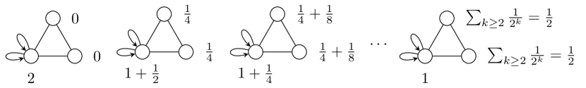
Figure 3: Steps of a divisible sandpile on a triangle with two added loops at the origin, starting with a mass of $2$ at the origin. The limit odometer at the origin is equal to $u(o)=1+\frac{1}{2}+\frac{1}{4}+\frac{1}{8}+\dots=2$.

3rd wave: For the 3rd wave we start with the final mass distribution of the second wave, that is $\mu_{0}^{\bm{(3)}}=\mu^{\bm{(2)}}$, and we use again the usual height function $h(x)\equiv 1$. The situation at the start of the $3$rd wave is depicted in Figure 4. Each of the outer small triangles behaves like the gadget depicted in Figure 3. Since the gray area is already filled, all mass that is sent to the inside has to come out again eventually. By symmetry, the amount of mass sent out to each boundary point will be the same, thus the whole interior has the same effect as adding two loops to each boundary point in $\partial B_{n}$. Since no more mass can accumulate in the interior, the odometer function in $B_{n}\setminus\partial B_{n}$ increases during the 3rd wave by a harmonic function which is equal to $2$ at all the boundary points $\partial B_{n}$. It follows that the odometer function of the 3rd wave is given by

$$u^{\bm{(3)}}(x)=2\mathds{1}_{\mathcal{B}_{n}}(x).$$

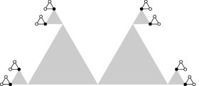
Figure 4: The sandpile at the start of the 3rd wave. The gray shaded region represents $B_{n}\setminus\partial B_{n}$ which is completely filled, i.e., $\mu^{(2)}\equiv 1$. The black dots $\bullet$ are the boundary points in $\partial B_{n}$ with sand height $2$. The white dots $\circ$ contain no sand.

To finish the argument we have to show that the sum of the odometers of the three waves $u^{\star}=u^{\bm{(1)}}+u^{\bm{(2)}}+u^{\bm{(3)}}$ is equal to $u_{n+1}$. For this we apply Lemma 3.10 to $u^{\star}$. By the induction hypothesis we have

$$\Delta u^{\bm{(1)}}(x) =\begin{cases}1-b_{n}\delta_{o}(x)\quad&\text{if }x\in B_{n}\setminus\partial{B_{n}},\\ 1/2&\text{if }x\in\partial{B_{n}},\\ 0&\text{if }x\not\in B_{n}.\end{cases}$$

For the odometers of the second and third wave we get

$$\Delta u^{\bm{(2)}}(x) =\begin{cases}-3/2\lvert\partial B_{n}\rvert\quad&\text{if }x=o,\\ 3/2&\text{if }x\in\partial{B_{n}},\\ 0&\text{otherwise}\end{cases}$$

and

$$\Delta u^{\bm{(3)}}(x) =\begin{cases}-1\quad&\text{if }x\in\partial B_{n},\\ 0&\text{if }x\in B_{n}\setminus\partial B_{n},\\ 1/2&\text{if }x\in\partial B_{n+1},\\ 1&\text{if }x\in\partial_{I}B_{n+1},\\ 0&\text{otherwise}.\end{cases}$$

Finally it follows by the linearity of the Laplacian that

$$\Delta u^{\star}(x) =\begin{cases}1-(b_{n}+3/2\lvert\partial B_{n}\rvert)\delta_{o}\quad&\text{if }x\in B_{n},\\ 1&\text{if }x\in\partial B_{n},\\ 1&\text{if }x\in\partial_{I}B_{n+1},\\ 1/2&\text{if }x\in\partial B_{n+1},\\ 0&\text{otherwise}\end{cases}$$

$$=\begin{cases}1-b_{n+1}\delta_{o}\quad&\text{if }x\in B_{n+1}\setminus\partial B_{n+1}\\ \ 1/2&\text{if }x\in\partial B_{n+1}\\ 0&\text{otherwise}\end{cases}$$

$$=\mu_{n+1}-\mu_{n+1,0}.$$

Moreover $\{x\in\mbox{{SG}}:u^{\star}(x)>0\}=B_{n}$. Thus Lemma 3.10 implies that $u^{\star}=u_{n+1}$, which finishes the inductive step. ∎

The main result Theorem 1.1 is just an application of the previous result.

Proof of Theorem 1.1..

The proof proceeds by the same wave argument as used in the proof of Theorem 4.2. In the first wave start with mass $b_{n}$ at the origin. By Theorem 4.2 the sandpile after this wave has exactly the shape $B_{n-1}$. For the second wave add the remaining mass $m-b_{n}<3/2\lvert\partial B_{n}\rvert$ at the origin. For the third wave there will be less then 2 mass at each vertex of $\partial B_{n}$. Hence the final sandpile cluster after the third wave will be a subset of $B_{n}$. ∎

5 Functions with constant Laplacian

For the proof of convergence of the divisible sandpile we have assumed the existence of a function $\ell:\mbox{{SG}}\to\mathbb{R}$ with $\Delta\ell(x)=1$ for all $x\in\mbox{{SG}}$. In this section we construct such a function with particularly nice properties and show how is it connected with the divisible sandpile model.

Recall that we are working with the representation of the SG, as given in the left part of Figure 1.

Definition 5.1.

A subset $T$ of SG is called a proper triangle of size $2^{k}$, if the subgraph induced by $T$ is isomorphic to $V_{k}^{+}$. If $T$ is a proper triangle, its extremal points $\partial T$ are either of the form $\partial T=\big{\{}a,a+(2^{k},0),a+(0,2^{k})\big{\}}$ for some $a\in\mbox{{SG}}^{+}$, or of the form $\partial T=\big{\{}a,a-(2^{k},0),a-(0,2^{k})\big{\}}$ for some $a\in\mbox{{SG}}^{-}$.

Definition 5.2.

Let $T$ be a proper triangle of size $2^{k}$ in SG for some $k\geq 1$, and let $\partial T=\big{\{}a,b,c)\big{\}}$, for some $a,b,c\in\mbox{{SG}}^{+}$. Without loss of generality we can assume $b=a+(2^{k},0)$ and $c=a+(0,2^{k})$. The midpoints of $T$ are then given by

$$A =(b+c)/2=a+(2^{k-1},2^{k-1})$$

$$B =(a+c)/2=a+(0,2^{k-1}),$$

$$C =(a+b)/2=a+(2^{k-1},0).$$

For proper triangles which are subsets of $\mbox{{SG}}^{-}$ the midpoints are defined analogously. See Figure 7 for a diagram of a proper triangle.

Definition 5.3.

A subset $B$ of SG is called a proper ball of size $2^{k}$, if the subgraph induced by $B$ is isomorphic to $V_{k}$. See Figure 7.

Next we define a simple function $\tilde{u}:\mbox{{SG}}^{+}\to\mathbb{R}$ which has Laplacian $1$ everywhere except at the origin $o$.

Definition 5.4.

Let $\tilde{u}:\mbox{{SG}}^{+}\to\mathbb{R}$ be the function defined by

$$\tilde{u}(x,0) =0\text{ for all }x\geq 0,$$

$$\tilde{u}(x,1) =2\text{ for all }x\geq 0\text{ s.t. }(x,1)\in\mbox{{SG}}^{+}$$

and $\Delta\tilde{u}(x,y)=1$, for all $x,y\in\mbox{{SG}}^{+}$ with $y\geq 1$.

Figure 5: The function $\tilde{u}$.

Remark 5.5.

It is easy to check that the definition implies that $\Delta\tilde{u}(x,0)=1$ for all $x\geq 1$.

A priori, it is not clear whether such a function $\tilde{u}$ is well defined, and if it is unique. This is what we prove next. In the proof of the next result we are going to use a generalized $\frac{1}{5}-\frac{2}{5}$ rule for functions with constant Laplacian in Sierpinski gasket graphs. In the fractal community, the $\frac{1}{5}-\frac{2}{5}$ rule for harmonic functions on the gasket SG is well-known, but we need it in a more general setting. The proof of the generalized $\frac{1}{5}-\frac{2}{5}$ rule for functions with constant Laplacian will be postponed for the Appendix, in Theorem A.1.

Theorem 5.6.

The function $\tilde{u}$ defined in Definition 5.4 is unique. Moreover $\tilde{u}(0,2^{k})=2\cdot 5^{k}$ for all $k\geq 0$.

Proof.

The set $V_{k}^{+}$ is a proper triangle of size $2^{k}$ in $\mbox{{SG}}^{+}$ with extremal points

$$\partial V_{k}^{+}=\big{\{}(0,0),(2^{k},0),(0,2^{k})\big{\}}.$$

By definition $\tilde{u}(0,0)=\tilde{u}(2^{k},0)=0$. Applying Theorem A.1(a) to the proper triangle $V_{k}^{+}$ gives

$$\tilde{u}(2^{k-1},0)=\frac{1}{5}\big{(}2\tilde{u}(2^{k},0)+2\tilde{u}(0,0)+\tilde{u}(0,2^{k})\big{)}-2\cdot 5^{k-1},$$

which together with $\tilde{u}(2^{k-1},0)=0$, implies $\tilde{u}(0,2^{k})=2\cdot 5^{k}.$

Again by the generalized $\frac{1}{5}-\frac{2}{5}$ rule in Theorem A.1, the values of $\tilde{u}$ on any proper triangle $T$ are uniquely determined by its values on the extremal points $\partial T$. Hence the existence and uniqueness of $\tilde{u}$ follows. ∎

See Figure 5 for a plot of the function $\tilde{u}$. Note that when we extend $\tilde{u}$ to the whole of SG by reflection at the origin we get a function with Laplacian equal to $1$ everywhere. That is

$$\ell(x,y)=\tilde{u}(\lvert x\rvert,\lvert y\rvert),$$

is a function with Laplacian 1 globally, as needed in Section 3.1. While $\ell$ is only used as a technical tool in Section 3.1 we will see below that the function $\tilde{u}$ has a much deeper link to the divisible sandpile on the Sierpinski gasket. We prove next some properties of $\tilde{u}$, in particular that it is integer valued and non-negative.

Lemma 5.7.

Let $T$ be a proper triangle of size $2^{k}$, $k\geq 1$, with extremal points $\partial T=\big{\{}a,b,c\big{\}}$ and midpoints $M=\big{\{}A,B,C\big{\}}$. Fix $m\in\mathbb{Z}$ and let $h$ be a function on SG with $\Delta h(z)=m$, for all $z\in T$. Assume the value of $h(z)$ is divisible by $2\cdot 5^{k}$ for all $z\in\partial T$. Then $h(w)$ is divisible by $2\cdot 5^{k-1}$, for all $w\in M$.

Proof.

By assumption $h(a)=2\cdot 5^{k}\tilde{a}$, $h(b)=2\cdot 5^{k}\tilde{b}$ and $h(c)=2\cdot 5^{k}\tilde{c}$ for some $\tilde{a},\tilde{b},\tilde{c}\in\mathbb{Z}$. By Theorem A.1(a), we can then determine the value of $h$ at midpoints:

$$h(A) =\frac{1}{5}\big{(}2\cdot 5^{k}\tilde{a}+4\cdot 5^{k}\tilde{b}+4\cdot 5^{k}\tilde{c}\big{)}-2\cdot 5^{k-1}m$$

$$=2\cdot 5^{k-1}\big{(}\tilde{a}+2\tilde{b}+2\tilde{c}-m\big{)}.$$

Hence $h(A)$ is divisible by $2\cdot 5^{k-1}$. The divisibility of $h(B)$ and $h(C)$ follows by symmetry. ∎

Theorem 5.8.

Let $T$ be an arbitrary proper triangle of size $2^{k}$, then for all extremal points $z\in\partial T$, $\tilde{u}(z)\in\mathbb{Z}$ and is divisible by $2\cdot 5^{k}$.

Proof.

Let $T$ be a proper triangle of size $2^{k}$, and let $l\geq 1$ be the smallest integer such that $T$ is a subset of $V_{l}^{+}$. By the definition of $\tilde{u}$ and Theorem 5.6 the value of $\tilde{u}$ at all extremal points of $V_{l}^{+}$ is divisible by $2\cdot 5^{l}$. The values of $\tilde{u}$ at the extremal points of $T$ can be computed by applying Theorem A.1a recursively at most $l-k$-times to the extremal points of $V_{k}^{+}$. The claim follows then from Lemma 5.7. ∎

As an immediate consequence we get the following.

Corollary 5.9.

$\tilde{u}(z)\in 2\mathbb{Z}$ for all $z\in\mbox{{SG}}^{+}$.

Theorem 5.10.

The function $\tilde{u}$ is non-negative on all of $\mbox{{SG}}^{+}$. Moreover $\tilde{u}(x,y)=0$ if and only if $y=0$.

Proof.

Let $a,b,c$ be the extremal points of a proper triangle of size $2^{k}$, and let $A,B,C$ be the midpoints of this triangle. By Lemma 5.7 there exists integers $\tilde{a},\tilde{b}$ and $\tilde{c}$ such that $\tilde{u}(a)=2\cdot 5^{k}\tilde{a}$, $\tilde{u}(b)=2\cdot 5^{k}\tilde{b}$ and $\tilde{u}(c)=2\cdot 5^{k}\tilde{c}$. Assume $\tilde{a},\tilde{b},\tilde{c}\geq 0$. It then follows again by Theorem A.1a that

$$\tilde{u}(A)=2\cdot 5^{k-1}\big{(}\tilde{a}+2\tilde{b}+2\tilde{c}-1\big{)}.$$

Then $\tilde{u}(A)<0$ if and only if $\tilde{a}=\tilde{b}=\tilde{c}=0$, and $\tilde{u}(A)=0$ if and only if $\tilde{a}=1$ and $\tilde{b}=\tilde{c}=0$. As in Lemma 5.7 we can compute all values of $\tilde{u}$ with the generalized $\frac{1}{5}-\frac{2}{5}$ rule starting from a set $V_{k}^{+}$, for some $k\geq 1$. Since we have already show in Theorem 5.6 that $\tilde{u}(0,2^{k})>0$, it follows by induction that $\tilde{u}(x,y)>0$ for all $(x,y)\in\mbox{{SG}}^{+}$ with $y>0$. ∎

5.1 Explicit construction of the odometer function

In section we will show that odometer of the divisible sandpile with initial sand configuration $\mu(x)=3^{k+1}\delta_{o}(x)$ is essentially given by an affine transformation of the function $\tilde{u}$. For this, we need to compute some particular values of $\tilde{u}$ explicitly.

Figure 6: The construction used in Lemma 5.11.

Lemma 5.11.

For all $k\geq 1$ we have $\tilde{u}(0,2^{k}-1)=\tilde{u}(1,2^{k}-1)=1-3^{k+1}+2\cdot 5^{k}$.

Proof.

Let $z=(0,2^{k})$ and define $l_{i}=(0,s_{i})$ and $r_{i}=(2^{k}-s_{i},s_{i})$, where $s_{i}=\sum_{j=1}^{i}2^{k-j}$, for all $i=0,\ldots,k$ (see Figure 6). In particular we have $l_{0}=(0,0)$, $r_{0}=(0,2^{k})$, $l_{k}=(0,2^{k}-1)$ and $r_{k}=(1,2^{k}-1)$. By the Theorem A.1a we get for all $i=1,\ldots,k$:

$$\begin{aligned} \tilde{u}(l_{i})&=\frac{1}{5}\big{(}\tilde{u}(r_{i-1})+2\tilde{u}(l_{i-1})+2\tilde{u}(z)\big{)}-2\cdot 5^{k-i},\\ \tilde{u}(r_{i})&=\frac{1}{5}\big{(}\tilde{u}(l_{i-1})+2\tilde{u}(r_{i-1})+2\tilde{u}(z)\big{)}-2\cdot 5^{k-i}.\end{aligned}$$ (6)

Since $\tilde{u}(l_{0})=\tilde{u}(r_{0})=0$ it follows by induction that $\tilde{u}(l_{i})=\tilde{u}(r_{i})$ for all $i=0,\ldots,k$. This simplifies the recursion (6) to

$$\begin{aligned} \tilde{u}(l_{i})&=\frac{1}{5}\big{(}3\tilde{u}(l_{i-1})+2\tilde{u}(z)\big{)}-2\cdot 5^{k-i}\\ &=\frac{3}{5}\tilde{u}(l_{i-1})+4\cdot 5^{k-1}-2\cdot 5^{k-i},\end{aligned}$$ (7)

where in the last line we used that $\tilde{u}(z)=2\cdot 5^{k}$ by Theorem 5.6. The linear recursion (7) has the explicit solution

$$\tilde{u}(l_{i})=5^{k-i}\big{(}1-3^{i+1}+2\cdot 5^{i}\big{)}.$$

Setting $i=k$ gives the result. ∎

Let $\psi_{k}:\mathbb{Z}^{2}\to\mathbb{Z}^{2}$ be the function given by $\psi_{k}(x,y)=(y,2^{k}-x-y)$, for all $k\geq 0$. We have $\psi_{k}(0,0)=(0,2^{k})$, $\psi_{k}(0,2^{k})=(2^{k},0)$ and $\psi(2^{k},0)=(0,0)$. That is, $\psi_{k}$ maps $\partial V_{k}^{+}=\big{\{}(0,0),(2^{k},0),(0,2^{k})\big{\}}$ onto itself. Moreover it is easy to check that $\psi_{k}$ is bijective on $V_{k}^{+}$ and acts as a rotation by $-120^{\circ}$ around the center of the biggest hole in $V_{k}^{+}$.

Theorem 5.12.

Let $u_{k}:\mbox{{SG}}\to\mathbb{R}_{\geq 0}$ be the odometer function of divisible sandpile on SG with initial mass distribution $\mu_{0}\equiv 3^{k+1}\delta_{(0,0)}$. Then for all $k\in\mathbb{N}_{0}$

$$u_{k}(x,y)=\begin{cases}(\tilde{u}\circ\psi_{k})(\lvert x\rvert,\lvert y\rvert),\quad&\text{ if }(x,y)\in B_{2^{k}},\\ 0,&\text{ otherwise}.\end{cases}$$ (8)

Moreover the sandpile cluster $\mathcal{S}=\big{\{}z\in\mbox{{SG}}:\>u_{k}(z)>0\big{\}}=B_{2^{k}-1}$.

Proof.

We check that the requirements in Lemma 3.10 are fulfilled for the function $u_{k}(x,y)$ defined in (8). By construction and Theorem 5.10, $u_{k}(z)>0$ if and only if $z\in B_{2^{k}-1}$. We need to check that $\Delta u_{k}(z)=1-\mu_{0}$ for all $z\in B_{2^{k}-1}$. For all $z\in B_{2^{k}-1}\setminus\{(0,0)\}$ is follows directly since $\Delta\tilde{u}(x,y)=1$ for all $y\geq 1$ by definition. For $z\in S_{2^{k}}$, we have $\Delta u(z)\in\{1/2,1\}$.

Thus we only need to calculate the Laplacian of $u_{k}$ at the origin. Since $\psi_{k}(0,0)=(0,2^{k})$ we have $u_{k}(0,0)=\tilde{u}(0,2^{k})=2\cdot 5^{k}$ by Theorem 5.6. For $z\sim(0,0)$ we have $\psi_{k}(z)\in\{(1,2^{k}-1),(0,2^{k}-1)\}$. Hence $u_{k}(z)=1-3^{k+1}+2\cdot 5^{k}$ by Lemma 5.11 for all $z\sim(0,0)$. Thus $\Delta u_{k}(0,0)=\frac{1}{4}\sum_{z\sim(0,0)}u_{k}(z)-u_{k}(0,0)=1-3^{k+1}+2\cdot 5^{k}-2\cdot 5^{k}=1-3^{k+1}$, which completes the proof. ∎

Remark 5.13.

Theorem 5.12 is a more explicit version of Theorem 4.2 for the special case $n=2^{k}$.

6 Open questions

The Sierpinski gasket graph SG is one of the simplest pre-fractals which has the property of being finitely ramified. This is very often used throughout the paper, especially when constructing explicitly the function with Laplacian $1$ on SG. It might be interesting to prove a limit shape theorem for the divisible sandpile model on the Sierpinski carpet graph, which is infinitely ramified. The Sierpinski carpet still has some special features (symmetry in particular), but is general enough so that one needs to develop more powerful techniques in order to analyze the behavior of the divisible sandpile model, model which turned out to be very helpful in proving limit shape theorems for the stochastic growth model internal DLA.

Appendix A Generalized $\frac{1}{5}-\frac{2}{5}$ rule

The following version of the $\frac{1}{5}-\frac{2}{5}$ rule for harmonic functions is probably known but since we did not find it in the literature in the form we need it here, we add a proof of this fact for completeness.

Theorem A.1 ($\frac{1}{5}-\frac{2}{5}$ rule for functions with constant Laplacian).

The following two properties are true for all $k\in\mathbb{N}$:

1. Let $T$ be a proper triangle of size $2^{k}$ and extremal points $\partial T=\big{\{}a,b,c\big{\}}$, and midpoints $\big{\{}A,B,C\big{\}}$ as in Figure 7. Let $h:\mbox{{SG}}\to\mathbb{R}$ be a function such that $\Delta h(x)=m$ for all $x\in T$. Then the values of $h$ at the midpoints are given by

   $$h(A) =\frac{1}{5}\big{(}h(a)+2h(b)+2h(c)\big{)}-2\cdot 5^{k-1}m,$$

   $$h(B) =\frac{1}{5}\big{(}2h(a)+h(b)+2h(c)\big{)}-2\cdot 5^{k-1}m,$$

   $$h(C) =\frac{1}{5}\big{(}2h(a)+2h(b)+h(c)\big{)}-2\cdot 5^{k-1}m.$$

2. Let $B$ be a proper ball of size $2^{k-1}$ with center $D$ and extremal points $\big{\{}d_{1},d_{2},d_{3},d_{4}\big{\}}$ as in Figure 7. Let $h:\mbox{{SG}}\to\mathbb{R}$ be a function such that $\Delta h(x)=m$ for all $x\in B$. Then the value of $h$ at the center point is given by

   $$h(D)=\frac{1}{4}\big{(}h(d_{1})+h(d_{2})+h(d_{3})+h(d_{4})\big{)}-5^{k-1}m.$$

Figure 7: Left: Proper triangle of size $2^{3}$, with extremal points $\{a,b,c\}$ and midpoints $\{A,B,C\}$. Right: Proper ball of size $2^{2}$ with center $D$ and extremal points $\{d_{1},d_{2},d_{3},d_{4}\}$.

Proof.

The proof goes by induction. First we consider the basis case $k=1$. To see relation (a) note the the function values at the midpoints are related to the values at the extremal points, by the following linear equation:

$$\left(\begin{array}[]{rrr}-4&1&1\\ 1&-4&1\\ 1&1&-4\end{array}\right)\cdot\begin{pmatrix}h(A)\\ h(B)\\ h(C)\end{pmatrix}+\begin{pmatrix}0&1&1\\ 1&0&1\\ 0&1&1\end{pmatrix}\cdot\begin{pmatrix}h(a)\\ h(b)\\ h(c)\end{pmatrix}=\begin{pmatrix}4m\\ 4m\\ 4m\end{pmatrix}.$$

Solving this equation gives relation (a). For $k=1$ relation (b) is just $\Delta h(D)=m$, and is thus true by assumption.

For the inductive step assume that both relations (a) and (b) are true for some $k\geq 1$. A proper triangle $T$ of size $2^{k+1}$ consists of three proper triangles of size $2^{k}$ which pairwise share one extremal point. See the left hand side of Figure 7. For each of these smaller triangles we can use relation (a) for the points $\alpha_{1},\alpha_{2},\alpha_{3}$ and $\beta_{1},\ldots,\beta_{6}$ in the notation of Figure 7. Moreover note that points $\big{\{}b,c,B,C\big{\}}$ are the extremal points of a proper ball of size $2^{k}$ with center $A$. Similarly $T$ contains two more proper balls of size $2^{k}$ with center points $B$ and $C$. We can apply relation (b) to these three proper balls. Let

$$\mathbf{h}=\big{(}h(A),h(B),h(C),h(\alpha_{1}),\ldots,h(\alpha_{3}),h(\beta_{1}),\ldots,h(\beta_{6})\big{)}^{T}$$

be the column vector of unknowns. This leads to a system of linear equations given by

$$\mathbf{M}\cdot\mathbf{h}=\mathbf{Y}\cdot\big{(}h(a),h(b),h(c),m\big{)}^{T},$$

where the matrices $\mathbf{M}$ and $\mathbf{Y}$ are given by

$$\mathbf{M}=\left(\begin{array}[]{rrr*{9}{>{\greytest}r}}0&-2&-2&5&0&0&0&0&0&0&0&0\\ -2&0&-2&0&5&0&0&0&0&0&0&0\\ -2&-2&0&0&0&5&0&0&0&0&0&0\\ 0&-2&-1&0&0&0&5&0&0&0&0&0\\ 0&-1&-2&0&0&0&0&5&0&0&0&0\\ -1&0&-2&0&0&0&0&0&5&0&0&0\\ -2&0&-1&0&0&0&0&0&0&5&0&0\\ -2&-1&0&0&0&0&0&0&0&0&5&0\\ -1&-2&0&0&0&0&0&0&0&0&0&5\\ 4&-1&-1&0&0&0&0&0&0&0&0&0\\ -1&4&-1&0&0&0&0&0&0&0&0&0\\ -1&-1&4&0&0&0&0&0&0&0&0&0\end{array}\right)\text{ and }\mathbf{Y}=\left(\begin{array}[]{*{4}{>{\greytest}r}}1&0&0&-2\cdot 5^{k}\\ 0&1&0&-2\cdot 5^{k}\\ 0&0&1&-2\cdot 5^{k}\\ 2&0&0&-2\cdot 5^{k}\\ 2&0&0&-2\cdot 5^{k}\\ 0&2&0&-2\cdot 5^{k}\\ 0&2&0&-2\cdot 5^{k}\\ 0&0&2&-2\cdot 5^{k}\\ 0&0&2&-2\cdot 5^{k}\\ 0&1&1&-4\cdot 5^{k}\\ 1&0&1&-4\cdot 5^{k}\\ 1&1&0&-4\cdot 5^{k}\end{array}\right).$$

Then the first three lines of $\mathbf{h}=\mathbf{M}^{-1}\cdot\mathbf{Y}\cdot\big{(}h(a),h(b),h(c),m\big{)}^{T}$ give relation (a) for $k+1$:

$$\begin{pmatrix}h(A)\\ h(B)\\ h(C)\end{pmatrix}=\frac{1}{5}\begin{pmatrix}1&2&2&-2\cdot 5^{k+1}\\ 2&1&2&-2\cdot 5^{k+1}\\ 2&2&1&-2\cdot 5^{k+1}\end{pmatrix}\cdot\begin{pmatrix}h(a)\\ h(b)\\ h(c)\\ m\end{pmatrix}$$

To prove the inductive step for relation (b), note that a proper ball of radius $2^{k}$ (see the right side of Figure 7), consists of two proper triangles of size $2^{k}$ with extremal points $\big{\{}D,d_{1},d_{2}\big{\}}$ resp. $\big{\{}D,d_{3},d_{4}\big{\}}$. Moreover $D$ is the center of a proper ball of size $2^{k-1}$ and extremal points $\big{\{}\gamma_{1},\gamma_{3},\gamma_{4},\gamma_{6}\}$, in the notation of Figure 7.

Let $\bm{\widetilde{h}}=\big{(}h(D),h(\gamma_{1}),\ldots,h(\gamma_{6})\big{)}^{T}$ be the vector of unknowns. Applying the induction hypothesis to these subsets leads to the linear equation

$$\bm{\widetilde{M}}\cdot\bm{\widetilde{h}}=\bm{\widetilde{Y}}\cdot\big{(}h(d_{1}),\ldots,h(d_{4}),m\big{)}^{T},$$

where the matrices $\bm{\widetilde{M}}$ and $\bm{\widetilde{Y}}$ are given by

$$\bm{\widetilde{M}}=\left(\begin{array}[]{*{7}{>{\greytest}r}}4&-1&\phantom{-}0&-1&-1&\phantom{-}0&-1\\ -2&5&0&0&0&0&0\\ -1&0&5&0&0&0&0\\ -2&0&0&5&0&0&0\\ -2&0&0&0&5&0&0\\ -1&0&0&0&0&5&0\\ -2&0&0&0&0&0&5\end{array}\right)\text{ and }\bm{\widetilde{Y}}=\left(\begin{array}[]{*{4}{>{\greytest}r}l}0&0&0&0&-4\cdot 5^{k-1}\\ 2&1&0&0&-2\cdot 5^{k}\\ 2&2&0&0&-2\cdot 5^{k}\\ 1&2&0&0&-2\cdot 5^{k}\\ 0&0&2&1&-2\cdot 5^{k}\\ 0&0&2&2&-2\cdot 5^{k}\\ 0&0&1&2&-2\cdot 5^{k}\end{array}\right).$$

Then the first line of $\bm{\widetilde{h}}=\bm{\widetilde{M}}^{-1}\cdot\bm{\widetilde{Y}}\cdot\big{(}h(d_{1}),\ldots,h(d_{4}),m\big{)}^{T}$ gives relation (b) for $k+1$:

$$h(D)=\left(\begin{array}[]{rrrrr}\dfrac{1}{4}&\dfrac{1}{4}&\dfrac{1}{4}&\dfrac{1}{4}&-5^{k}\end{array}\right)\cdot\begin{pmatrix}h(d_{1})\\ \vdots\\ h(d_{4})\\ m\end{pmatrix},$$

and this finishes the proof. ∎

Acknowledgements.

The research of Wilfried Huss was supported by the Austrian Science Fund (FWF): J3628-N26 and P25510-N26. The research of Ecaterina Sava-Huss was supported by the Austrian Science Fund (FWF): J3575-N26.

Wilfried Huss, Institute of Discrete Mathematics, Graz University of Technology, 8010 Graz, Austria. huss@math.tugraz.at
http://www.math.tugraz.at/~huss

Ecaterina Sava-Huss, Institute of Discrete Mathematics, Graz University of Technology, 8010 Graz, Austria. sava-huss@tugraz.at
http://www.math.tugraz.at/~sava

References

• [CHSHT17] Joeย P. Chen, Wilfried Huss, Ecaterina Sava-Huss, and Alexander Teplyaev. Internal DLA on Sierpinski gasket graphs. 2017, arXiv:1702.04017.
• [CSC09] Tullio Ceccherini-Silberstein and Michel Coornaert. A note on Laplace operators on groups. In Limits of graphs in group theory and computer science, pages 37โ€“40. EPFL Press, Lausanne, 2009.
• [FL13] Tobias Friedrich and Lionel Levine. Fast simulation of large-scale growth models. Random Structures Algorithms, 42(2):185โ€“213, 2013, arXiv:1006.1003.
• [HS11] Wilfried Huss and Ecaterina Sava. Rotor-router aggregation on the comb. Electron. J. Combin., 18(1):Paper 224, 23, 2011, arXiv:1103.4797.
• [HS12] Wilfried Huss and Ecaterina Sava. Internal aggregation models on comb lattices. Electron. J. Probab., 17:no. 30, 21, 2012, arXiv:1106.4468.
• [KL10] Wouter Kager and Lionel Levine. Rotor-router aggregation on the layered square lattice. Electron. J. Combin., 17(1):Research Paper 152, 16, 2010, arXiv:1003.4017.
• [Kum14] Takashi Kumagai. Random Walks on Disordered Media and their Scaling Limits. Springer International Publishing, 2014.
• [Lev09] Lionel Levine. The sandpile group of a tree. European Journal of Combinatorics, 30(4):1026 โ€“ 1035, 2009, arXiv:math/0703868.
• [LP09] Lionel Levine and Yuval Peres. Strong spherical asymptotics for rotor-router aggregation and the divisible sandpile. Potential Anal., 30(1):1โ€“27, 2009, arXiv:0704.0688.
• [LP16] L.ย Levine and Y.ย Peres. Laplacian growth, sandpiles and scaling limits. ArXiv e-prints, November 2016, arXiv:1611.00411.