Dynamic Word Embeddings

Abstract

We present a probabilistic language model for time-stamped text data which tracks the semantic evolution of individual words over time. The model represents words and contexts by latent trajectories in an embedding space. At each moment in time, the embedding vectors are inferred from a probabilistic version of word2vec (Mikolov et al., 2013b). These embedding vectors are connected in time through a latent diffusion process. We describe two scalable variational inference algorithms—skip-gram smoothing and skip-gram filtering—that allow us to train the model jointly over all times; thus learning on all data while simultaneously allowing word and context vectors to drift. Experimental results on three different corpora demonstrate that our dynamic model infers word embedding trajectories that are more interpretable and lead to higher predictive likelihoods than competing methods that are based on static models trained separately on time slices.

1 Introduction

Language evolves over time and words change their meaning due to cultural shifts, technological inventions, or political events. We consider the problem of detecting shifts in the meaning and usage of words over a given time span based on text data. Capturing these semantic shifts requires a dynamic language model.

Word embeddings are a powerful tool for modeling semantic relations between individual words (Bengio et al., 2003; Mikolov et al., 2013a; Pennington et al., 2014; Mnih & Kavukcuoglu, 2013; Levy & Goldberg, 2014; Vilnis & McCallum, 2014; Rudolph et al., 2016). Word embeddings model the distribution of words based on their surrounding words in a training corpus, and summarize these statistics in terms of low-dimensional vector representations. Geometric distances between word vectors reflect semantic similarity (Mikolov et al., 2013a) and difference vectors encode semantic and syntactic relations (Mikolov et al., 2013c), which shows that they are sensible representations of language. Pre-trained word embeddings are useful for various supervised tasks, including sentiment analysis (Socher et al., 2013b), semantic parsing (Socher et al., 2013a), and computer vision (Fu & Sigal, 2016). As unsupervised models, they have also been used for the exploration of word analogies and linguistics (Mikolov et al., 2013c).

Word embeddings are currently formulated as static models, which assumes that the meaning of any given word is the same across the entire text corpus. In this paper, we propose a generalization of word embeddings to sequential data, such as corpora of historic texts or streams of text in social media.

Current approaches to learning word embeddings in a dynamic context rely on grouping the data into time bins and training the embeddings separately on these bins (Kim et al., 2014; Kulkarni et al., 2015; Hamilton et al., 2016). This approach, however, raises three fundamental problems. First, since word embedding models are non-convex, training them twice on the same data will lead to different results. Thus, embedding vectors at successive times can only be approximately related to each other, and only if the embedding dimension is large (Hamilton et al., 2016). Second, dividing a corpus into separate time bins may lead to training sets that are too small to train a word embedding model. Hence, one runs the risk of overfitting to few data whenever the required temporal resolution is fine-grained, as we show in the experimental section. Third, due to the finite corpus size the learned word embedding vectors are subject to random noise. It is difficult to disambiguate this noise from systematic semantic drifts between subsequent times, in particular over short time spans, where we expect only minor semantic drift.

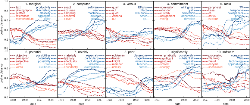
Figure 1: Evolution of the $10$ words that changed the most in cosine distance from 1850 to 2008 on Google books, using skip-gram filtering (proposed). Red (blue) curves correspond to the five closest words at the beginning (end) of the time span, respectively.

In this paper, we circumvent these problems by introducing a dynamic word embedding model. Our contributions are as follows:

• We derive a probabilistic state space model where word and context embeddings evolve in time according to a diffusion process. It generalizes the skip-gram model (Mikolov et al., 2013b; Barkan, 2017) to a dynamic setup, which allows end-to-end training. This leads to continuous embedding trajectories, smoothes out noise in the word-context statistics, and allows us to share information across all times.

• We propose two scalable black-box variational inference algorithms (Ranganath et al., 2014; Rezende et al., 2014) for filtering and smoothing. These algorithms find word embeddings that generalize better to held-out data. Our smoothing algorithm carries out efficient black-box variational inference for structured Gaussian variational distributions with tridiagonal precision matrices, and applies more broadly.

• We analyze three massive text corpora that span over long periods of time. Our approach allows us to automatically find the words whose meaning changes the most. It results in smooth word embedding trajectories and therefore allows us to measure and visualize the continuous dynamics of the entire embedding cloud as it deforms over time.

Figure 1 exemplifies our method. The plot shows a fit of our dynamic skip-gram model to Google books (we give details in section 5). We show the ten words whose meaning changed most drastically in terms of cosine distance over the last $150$ years. We thereby automatically discover words such as “computer” or “radio” whose meaning changed due to technological advances, but also words like “peer” and “notably” whose semantic shift is less obvious.

Our paper is structured as follows. In section 2 we discuss related work, and we introduce our model in section 3. In section 4 we present two efficient variational inference algorithms for our dynamic model. We show experimental results in section 5. Section 6 summarizes our findings.

2 Related Work

Probabilistic models that have been extended to latent time series models are ubiquitous (Blei & Lafferty, 2006; Wang et al., 2008; Sahoo et al., 2012; Gultekin & Paisley, 2014; Charlin et al., 2015; Ranganath et al., 2015; Jerfel et al., 2017), but none of them relate to word embeddings. The closest of these models is the dynamic topic model (Blei & Lafferty, 2006; Wang et al., 2008), which learns the evolution of latent topics over time. Topic models are based on bag-of-word representations and thus treat words as symbols without modelling their semantic relations. They therefore serve a different purpose.

Mikolov et al. (2013a, b) proposed the skip-gram model with negative sampling (word2vec) as a scalable word embedding approach that relies on stochastic gradient descent. This approach has been formulated in a Bayesian setup (Barkan, 2017), which we discuss separately in section 3.1. These models, however, do not allow the word embedding vectors to change over time.

Several authors have analyzed different statistics of text data to analyze semantic changes of words over time (Mihalcea & Nastase, 2012; Sagi et al., 2011; Kim et al., 2014; Kulkarni et al., 2015; Hamilton et al., 2016). None of them explicitly model a dynamical process; instead, they slice the data into different time bins, fit the model separately on each bin, and further analyze the embedding vectors in post-processing. By construction, these static models can therefore not share statistical strength across time. This limits the applicability of static models to very large corpora.

Most related to our approach are methods based on word embeddings. Kim et al. (2014) fit word2vec separately on different time bins, where the word vectors obtained for the previous bin are used to initialize the algorithm for the next time bin. The bins have to be sufficiently large and the found trajectories are not as smooth as ours, as we demonstrate in this paper. Hamilton et al. (2016) also trained word2vec separately on several large corpora from different decades. If the embedding dimension is large enough (and hence the optimization problem less non-convex), the authors argue that word embeddings at nearby times approximately differ by a global rotation in addition to a small semantic drift, and they approximately compute this rotation. As the latter does not exist in a strict sense, it is difficult to distinguish artifacts of the approximate rotation from a true semantic drift. As discussed in this paper, both variants result in trajectories which are noisier.

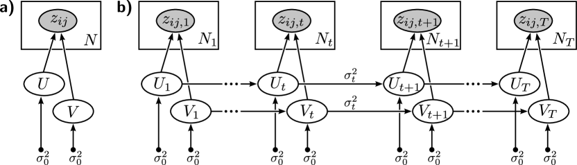
Figure 2: a) Bayesian skip-gram model (Barkan, 2017). b) The dynamic skip-gram model (proposed) connects $T$ copies of the Bayesian skip-gram model via a latent time series prior on the embeddings.

3 Model

We propose the dynamic skip-gram model, a generalization of the skip-gram model (word2vec) (Mikolov et al., 2013b) to sequential text data. The model finds word embedding vectors that continuously drift over time, allowing to track changes in language and word usage over short and long periods of time. Dynamic skip-gram is a probabilistic model which combines a Bayesian version of the skip-gram model (Barkan, 2017) with a latent time series. It is jointly trained end-to-end and scales to massive data by means of approximate Bayesian inference.

The observed data consist of sequences of words from a finite vocabulary of size $L$. In section 3.1, all sequences (sentences from books, articles, or tweets) are considered time-independent; in section 3.2 they will be associated with different time stamps. The goal is to maximize the probability of every word that occurs in the data given its surrounding words within a so-called context window. As detailed below, the model learns two vectors $u_{i},v_{i}\in\mathbb{R}^{d}$ for each word $i$ in the vocabulary, where $d$ is the embedding dimension. We refer to $u_{i}$ as the word embedding vector and to $v_{i}$ as the context embedding vector.

3.1 Bayesian Skip-Gram Model

The Bayesian skip-gram model (Barkan, 2017) is a probabilistic version of word2vec (Mikolov et al., 2013b) and forms the basis of our approach. The graphical model is shown in Figure 2a). For each pair of words $i,j$ in the vocabulary, the model assigns probabilities that word $i$ appears in the context of word $j$. This probability is $\sigma(u_{i}^{\top}v_{j})$ with the sigmoid function $\sigma(x)=1/(1+e^{-x})$. Let $z_{ij}\in\{0,1\}$ be an indicator variable that denotes a draw from that probability distribution, hence $p(z_{ij}=1)=\sigma(u_{i}^{\top}v_{j})$. The generative model assumes that many word-word pairs $(i,j)$ are uniformly drawn from the vocabulary and tested for being a word-context pair; hence a separate random indicator $z_{ij}$ is associated with each drawn pair.

Focusing on words and their neighbors in a context window, we collect evidence of word-word pairs for which $z_{ij}=1$. These are called the positive examples. Denote $n^{+}_{ij}$ the number of times that a word-context pair $(i,j)$ is observed in the corpus. This is a sufficient statistic of the model, and its contribution to the likelihood is $p(n^{+}_{ij}|u_{i},v_{j})=\sigma(u_{i}^{\top}v_{j})^{n^{+}_{ij}}$. However, the generative process also assumes the possibility to reject word-word pairs if $z_{ij}=0$. Thus, one needs to construct a fictitious second training set of rejected word-word pairs, called negative examples. Let the corresponding counts be $n^{-}_{ij}$. The total likelihood of both positive and negative examples is then

$$p(n^{+},n^{-}|U,V)=\prod_{i,j=1}^{L}\sigma(u_{i}^{\top}v_{j})^{n^{+}_{ij}}\sigma(-u_{i}^{\top}v_{j})^{n^{-}_{ij}}.$$ (1)

Above we used the antisymmetry $\sigma(-x)=1-\sigma(x)$. In our notation, dropping the subscript indices for $n^{+}$ and $n^{-}$ denotes the entire $L\times L$ matrices, $U=(u_{1},\cdots,u_{L})\in{\mathbb{R}}^{d\times L}$ is the matrix of all word embedding vectors, and $V$ is defined analogously for the context vectors. To construct negative examples, one typically chooses $n^{-}_{ij}\propto P(i)P(j)^{3/4}$ (Mikolov et al., 2013b), where $P(i)$ is the frequency of word $i$ in the training corpus. Thus, $n^{-}$ is well-defined up to a constant factor which has to be tuned.

Defining $n^{\pm}=(n^{+},n^{-})$ the combination of both positive and negative examples, the resulting log likelihood is

$$\log p(n^{\pm}|U,V)=\\ \sum_{i,j=1}^{L}\big{(}n^{+}_{ij}\log\sigma(u_{i}^{\top}v_{j})+n^{-}_{ij}\log\sigma(-u_{i}^{\top}v_{j})\big{)}.$$ (2)

This is exactly the objective of the (non-Bayesian) skip-gram model, see (Mikolov et al., 2013b). The count matrices $n^{+}$ and $n^{-}$ are either pre-computed for the entire corpus, or estimated based on stochastic subsamples from the data in a sequential way, as done by word2vec. Barkan (2017) gives an approximate Bayesian treatment of the model with Gaussian priors on the embeddings.

3.2 Dynamic Skip-Gram Model

The key extension of our approach is to use a Kalman filter as a prior for the time-evolution of the latent embeddings (Welch & Bishop, 1995). This allows us to share information across all times while still allowing the embeddings to drift.

Notation.

We consider a corpus of $T$ documents which were written at time stamps $\tau_{1}<\ldots<\tau_{T}$. For each time step $t\in\{1,\ldots,T\}$ the sufficient statistics of word-context pairs are encoded in the $L\times L$ matrices $n^{+}_{t},n^{-}_{t}$ of positive and negative counts with matrix elements $n^{+}_{ij,t}$ and $n^{-}_{ij,t}$, respectively. Denote $U_{t}=(u_{1,t},\cdots,u_{L,t})\in{\mathbb{R}}^{d\times L}$ the matrix of word embeddings at time $t$, and define $V_{t}$ correspondingly for the context vectors. Let $U,V\in{\mathbb{R}}^{T\times d\times L}$ denote the tensors of word and context embeddings across all times, respectively.

Model.

The graphical model is shown in Figure 2b). We consider a diffusion process of the embedding vectors over time. The variance $\sigma_{t}^{2}$ of the transition kernel is

$$\sigma_{t}^{2}=D(\tau_{t+1}-\tau_{t}),$$ (3)

where $D$ is a global diffusion constant and $(\tau_{t+1}-\tau_{t})$ is the time between subsequent observations (Welch & Bishop, 1995). At every time step $t$, we add an additional Gaussian prior with zero mean and variance $\sigma_{0}^{2}$ which prevents the embedding vectors from growing very large, thus

$$p(U_{t+1}|U_{t})\propto{\cal N}(U_{t},\sigma_{t}^{2})\,{\cal N}(0,\sigma_{0}^{2}).$$ (4)

Computing the normalization, this results in

$$U_{t+1}|U_{t}\sim{\cal N}\left(\frac{U_{t}}{1+\sigma_{t}^{2}/\sigma_{0}^{2}},\frac{1}{\sigma_{t}^{-2}+\sigma_{0}^{-2}}I\right),$$ (5)

$$V_{t+1}|V_{t}\sim{\cal N}\left(\frac{V_{t}}{1+\sigma_{t}^{2}/\sigma_{0}^{2}},\frac{1}{\sigma_{t}^{-2}+\sigma_{0}^{-2}}I\right).$$ (6)

In practice, $\sigma_{0}\gg\sigma_{t}$, so the damping to the origin is very weak. This is also called Ornstein-Uhlenbeck process (Uhlenbeck & Ornstein, 1930). We recover the Wiener process for $\sigma_{0}\rightarrow\infty$, but $\sigma_{0}<\infty$ prevents the latent time series from diverging to infinity. At time index $t=1$, we define $p(U_{1}|U_{0})\equiv{\cal N}(0,\sigma_{0}^{2}I)$ and do the same for $V_{1}$.

Our joint distribution factorizes as follows:

$$p(n^{\pm},U,V)=\prod_{t=0}^{T-1}p(U_{t+1}|U_{t})\,p(V_{t+1}|V_{t})\\ \times\prod_{t=1}^{T}\prod_{i,j=1}^{L}p(n_{ij,t}^{\pm}|u_{i,t},v_{j,t})$$ (7)

The prior model enforces that the model learns embedding vectors which vary smoothly across time. This allows to associate words unambiguously with each other and to detect semantic changes. The model efficiently shares information across the time domain, which allows to fit the model even in setups where the data at every given point in time are small, as long as the data in total are large.

4 Inference

We discuss two scalable approximate inference algorithms. Filtering uses only information from the past; it is required in streaming applications where the data are revealed to us sequentially. Smoothing is the other inference method, which learns better embeddings but requires the full sequence of documents ahead of time.

In Bayesian inference, we start by formulating a joint distribution (Eq. 7) over observations $n^{\pm}$ and parameters $U$ and $V$, and we are interested in the posterior distribution over parameters conditioned on observations,

$$p(U,V|n^{\pm})=\frac{p(n^{\pm},U,V)}{\int p(n^{\pm},U,V)\,dUdV}$$ (8)

The problem is that the normalization is intractable. In variational inference (VI) (Jordan et al., 1999; Blei et al., 2016) one sidesteps this problem and approximates the posterior with a simpler variational distribution $q_{\lambda}(U,V)$ by minimizing the Kullback-Leibler (KL) divergence to the posterior. Here, $\lambda$ summarizes all parameters of the variational distribution, such as the means and variances of a Gaussian, see below. Minimizing the KL divergence is equivalent to optimizing the evidence lower bound (ELBO) (Blei et al., 2016),

$$\mathcal{L}(\lambda)=\mathbb{E}_{q_{\lambda}}[\log p(n^{\pm},U,V)]-\mathbb{E}_{q_{\lambda}}[\log q_{\lambda}(U,V)].$$ (9)

For a restricted class of models, the ELBO can be computed in closed-form (Hoffman et al., 2013). Our model is non-conjugate and requires instead black-box VI using the reparameterization trick (Rezende et al., 2014; Kingma & Welling, 2014).

4.1 Skip-Gram Filtering

In many applications such as streaming, the data arrive sequentially. Thus, we can only condition our model on past and not on future observations. We will first describe inference in such a (Kalman) filtering setup (Kalman et al., 1960; Welch & Bishop, 1995).

In the filtering scenario, the inference algorithm iteratively updates the variational distribution $q$ as evidence from each time step $t$ becomes available. We thereby use a variational distribution that factorizes across all times, $q(U,V)=\prod_{t=1}^{T}q(U_{t},V_{t})$ and we update the variational factor at a given time $t$ based on the evidence at time $t$ and the approximate posterior of the previous time step. Furthermore, at every time $t$ we use a fully-factorized distribution:

$$q(U_{t},V_{t})=\prod_{i=1}^{L}\mathcal{N}(u_{i,t};\mu_{ui,t},\Sigma_{ui,t})\,\mathcal{N}(v_{i,t};\mu_{vi,t}.\Sigma_{vi,t}),$$

The variational parameters are the means $\mu_{ui,t},\mu_{vi,t}\in\mathbb{R}^{d}$ and the covariance matrices $\Sigma_{ui,t}$ and $\Sigma_{vi,t}$, which we restrict to be diagonal (mean-field approximation).

We now describe how we sequentially compute $q(U_{t},V_{t})$ and use the result to proceed to the next time step. As other Markovian dynamical systems, our model assumes the following recursion,

$$p(U_{t},V_{t}|n_{1:t}^{\pm})\propto p(n_{t}^{\pm}|U_{t},V_{t})\,p(U_{t},V_{t}|n_{1:t-1}^{\pm}).$$ (10)

Within our variational approximation, the ELBO (Eq. 9) therefore separates into a sum of $T$ terms, $\mathcal{L}=\sum_{t}\mathcal{L}_{t}$ with

$$\mathcal{L}_{t}=\mathbb{E}[\log p(n_{t}^{\pm}|U_{t},V_{t})]+\mathbb{E}[\log p(U_{t},V_{t}|n^{\pm}_{1:t-1})]\\ -\mathbb{E}[\log q(U_{t},V_{t})],$$ (11)

where all expectations are taken under $q(U_{t},V_{t})$. We compute the entropy term $-\mathbb{E}[\log q]$ in Eq. 11 analytically and estimate the gradient of the log likelihood by sampling from the variational distribution and using the reparameterization trick (Kingma & Welling, 2014; Salimans & Kingma, 2016). However, the second term of Eq. 11, containing the prior at time $t$, is still intractable. We approximate the prior as

$$p(U_{t},V_{t}|n^{\pm}_{1:t-1})\equiv\\ \mathbb{E}_{p(U_{t-1},V_{t-1}|n^{\pm}_{1:t-1})}\big{[}p(U_{t},V_{t}|U_{t-1},V_{t-1})\big{]}\\ \approx\mathbb{E}_{q(U_{t-1},V_{t-1})}\big{[}p(U_{t},V_{t}|U_{t-1},V_{t-1})\big{]}.\,$$ (12)

The remaining expectation involves only Gaussians and can be carried-out analytically. The resulting approximate prior is a fully factorized distribution $p(U_{t},V_{t}|n^{\pm}_{1:t-1})\approx\prod_{i=1}^{L}\mathcal{N}(u_{i,t};\tilde{\mu}_{ui,t},\tilde{\Sigma}_{ui,t})\,\mathcal{N}(v_{i,t};\tilde{\mu}_{vi,t},\tilde{\Sigma}_{vit})$ with

$$\begin{split}\tilde{\mu}_{ui,t}&=\tilde{\Sigma}_{ui,t}\left(\Sigma_{ui,t-1}+\sigma_{t}^{2}I\right)^{-1}\mu_{ui,t-1};\\ \tilde{\Sigma}_{ui,t}&=\left[\left(\Sigma_{ui,t-1}+\sigma_{t}^{2}I\right)^{-1}+(1/\sigma_{0}^{2})I\right]^{-1}.\end{split}$$ (13)

Analogous update equations hold for $\tilde{\mu}_{vi,t}$ and $\tilde{\Sigma}_{vi,t}$. Thus, the second contribution in Eq. 11 (the prior) yields a closed-form expression. We can therefore compute its gradient.

4.2 Skip-Gram Smoothing

In contrast to filtering, where inference is conditioned on past observations until a given time $t$, (Kalman) smoothing performs inference based on the entire sequence of observations $n^{\pm}_{1{:}T}$. This approach results in smoother trajectories and typically higher likelihoods than with filtering, because evidence is used from both future and past observations.

Besides the new inference scheme, we also use a different variational distribution. As the model is fitted jointly to all time steps, we are no longer restricted to a variational distribution that factorizes in time. For simplicity we focus here on the variational distribution for the word embeddings $U$; the context embeddings $V$ are treated identically. We use a factorized distribution over both embedding space and vocabulary space,

$$q(U_{1:T})=\prod_{i=1}^{L}\prod_{k=1}^{d}q(u_{ik,1:T}).$$ (14)

In the time domain, our variational approximation is structured. To simplify the notation we now drop the indices for words $i$ and embedding dimension $k$, hence we write $q(u_{1:T})$ for $q(u_{ik,1:T})$ where we focus on a single factor. This factor is a multivariate Gaussian distribution in the time domain with tridiagonal precision matrix $\Lambda$,

$$q(u_{1:T})={\cal N}(\mu,\Lambda^{-1})$$ (15)

Both the means $\mu=\mu_{1:T}$ and the entries of the tridiagonal precision matrix $\Lambda\in\mathbb{R}^{T\times T}$ are variational parameters. This gives our variational distribution the interpretation of a posterior of a Kalman filter (Blei & Lafferty, 2006), which captures correlations in time.

We fit the variational parameters by training the model jointly on all time steps, using black-box VI and the reparameterization trick. As the computational complexity of an update step scales as $\Theta(L^{2})$, we first pretrain the model by drawing minibatches of $L^{\prime}<L$ random words and $L^{\prime}$ random contexts from the vocabulary (Hoffman et al., 2013). We then switch to the full batch to reduce the sampling noise. Since the variational distribution does not factorize in the time domain we always include all time steps $\{1,\ldots,T\}$ in the minibatch.

We also derive an efficient algorithm that allows us to estimate the reparametrization gradient using $\Theta(T)$ time and memory, while a naive implementation of black-box variational inference with our structured variational distribution would require $\Theta(T^{2})$ of both resources. The main idea is to parametrize $\Lambda=B^{\top}B$ in terms of its Cholesky decomposition $B$, which is bidiagonal (Kılıç & Stanica, 2013), and to express gradients of $B^{-1}$ in terms of gradients of $B$. We use mirror ascent (Ben-Tal et al., 2001; Beck & Teboulle, 2003) to enforce positive definiteness of $B$. The algorithm is detailed in our supplementary material.

5 Experiments

We evaluate our method on three time-stamped text corpora. We demonstrate that our algorithms find smoother embedding trajectories than methods based on a static model. This allows us to track semantic changes of individual words by following nearest-neighbor relations over time. In our quantitative analysis, we find higher predictive likelihoods on held-out data compared to our baselines.

Algorithms and Baselines.

We report results from our proposed algorithms from section 4 and compare against baselines from section 2:

• SGI denotes the non-Bayesian skip-gram model with independent random initializations of word vectors (Mikolov et al., 2013b). We used our own implementation of the model by dropping the Kalman filtering prior and point-estimating embedding vectors. Word vectors at nearby times are made comparable by approximate orthogonal transformations, which corresponds to Hamilton et al. (2016).

• SGP denotes the same approach as above, but with word and context vectors being pre-initialized with the values from the previous year, as in Kim et al. (2014).

• DSG-F: dynamic skip-gram filtering (proposed).

• DSG-S: dynamic skip-gram smoothing (proposed).

Data and preprocessing.

Our three corpora exemplify opposite limits both in the covered time span and in the amount of text per time step.

• We used data from the Google books corpus (Michel et al., 2011) from the last two centuries ($T=209$). This amounts to $5$ million digitized books and approximately $10^{10}$ observed words. The corpus consists of $n$-gram tables with $n\in\{1,\ldots,5\}$, annotated by year of publication. We considered the years from $1800$ to $2008$ (the latest available). In $1800$, the size of the data is approximately $\sim 7\cdot 10^{7}$ words. We used the $5$-gram counts, resulting in a context window size of $4$.

• We used the “State of the Union” (SoU) addresses of U.S. presidents, which spans more than two centuries, resulting in $T=230$ different time steps and approximately $10^{6}$ observed words. Some presidents gave both a written and an oral address; if these were less than a week apart we concatenated them and used the average date. We converted all words to lower case and constructed the positive sample counts $n^{+}_{ij}$ using a context window size of $4$.

• We used a Twitter corpus of news tweets for $21$ randomly drawn dates from $2010$ to $2016$. The median number of tweets per day is $722$. We converted all tweets to lower case and used a context window size of $4$, which we restricted to stay within single tweets.

Hyperparameters.

The vocabulary for each corpus was constructed from the $10{,}000$ most frequent words throughout the given time period. In the Google books corpus, the number of words per year grows by a factor of $200$ from the year $1800$ to $2008$. To avoid that the vocabulary is dominated by modern words we normalized the word frequencies separately for each year before adding them up.

For the Google books corpus, we chose the embedding dimension $d=200$, which was also used in Kim et al. (2014). We set $d=100$ for SoU and Twitter, as $d=200$ resulted in overfitting on these much smaller corpora. The ratio $\eta=\sum_{ij}n_{ij,t}^{-}/\sum_{ij}n_{ij,t}^{+}$ of negative to positive word-context pairs was $\eta=1$. The precise construction of the matrices $n^{\pm}_{t}$ is explained in the supplementary material. We used the global prior variance $\sigma_{0}^{2}=1$ for all corpora and all algorithms, including the baselines. The diffusion constant $D$ controls the time scale on which information is shared between time steps. The optimal value for $D$ depends on the application. A single corpus may exhibit semantic shifts of words on different time scales, and the optimal choice for $D$ depends on the time scale in which one is interested. We used $D=10^{-3}$ per year for Google books and SoU, and $D=1$ per year for the Twitter corpus, which spans a much shorter time range. In the supplementary material, we provide details of the optimization procedure.

Qualitative results.

We show that our approach results in smooth word embedding trajectories on all three corpora. We can automatically detect words that undergo significant semantic changes over time.

Figure 3: Word embeddings over a sequence of years trained on Google books, using DSG-F (proposed, top row) and compared to the static method by Hamilton et al. (2016) (bottom). We used dynamic t-SNE (Rauber et al., 2016) for dimensionality reduction. Colored lines in the second to fourth column indicate the trajectories from the previous year. Our method infers smoother trajectories with only few words that move quickly. Figure 4 shows that these effects persist in the original embedding space.

Figure 4: Histogram of distances between word vectors in the year 1998 and their positions in subsequent years (colors). DSG-F (top panel) displays a continuous growth of these distances over time, indicating a directed motion. In contrast, in SGP (middle) (Kim et al., 2014) and SGI (bottom) (Hamilton et al., 2016), the distribution of distances jumps from the first to the second year but then remains largely stationary, indicating absence of a directed drift; i.e. almost all motion is random.

Figure 1 in the introduction shows a fit of the dynamic skip-gram filtering algorithm to the Google books corpus. Here, we show the ten words whose word vectors change most drastically over the last $150$ years in terms of cosine distance. Figure 3 visualizes word embedding clouds over four subsequent years of Google books, where we compare DSG-F against SGI. We mapped the normalized embedding vectors to two dimensions using dynamic t-SNE (Rauber et al., 2016) (see supplement for details). Lines indicate shifts of word vectors relative to the preceding year. In our model only few words change their position in the embedding space rapidly, while embeddings using SGI show strong fluctuations, making the cloud’s motion hard to track.

Figure 4 visualizes the smoothness of the trajectories directly in the embedding space (without the projection to two dimensions). We consider differences between word vectors in the year 1998 and the subsequent 10 years. In more detail, we compute histograms of the Euclidean distances $||u_{it}-u_{i,t+\delta}||$ over the word indexes $i$, where $\delta=1,\dots,10$ (as discussed previously, SGI uses a global rotation to optimally align embeddings first). In our model, embedding vectors gradually move away from their original position as time progresses, indicating a directed motion. In contrast, both baseline models show only little directed motion after the first time step, suggesting that most temporal changes are due to finite-size fluctuations of $n^{\pm}_{ij,t}$. Initialization schemes alone, thus, seem to have a minor effect on smoothness.

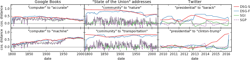
Figure 5: Smoothness of word embedding trajectories, compared across different methods. We plot the cosine distance between two words (see captions) over time. High values indicate similarity. Our methods (DSG-S and DSG-F) find more interpretable trajectories than the baselines (SGI and SGP). The different performance is most pronounced when the corpus is small (SoU and Twitter).

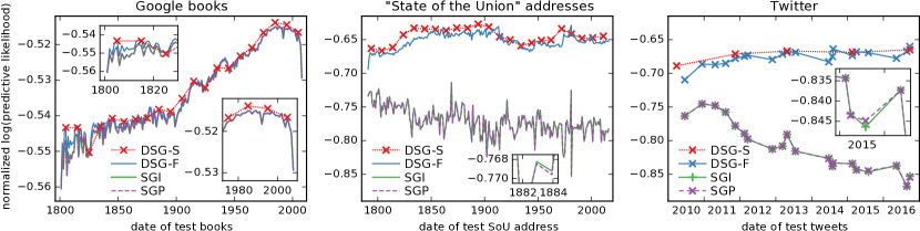
Figure 6: Predictive log-likelihoods (Eq. 16) for two proposed versions of the dynamic skip-gram model (DSG-F & DSG-S) and two competing methods SGI (Hamilton et al., 2016) and SGP (Kim et al., 2014) on three different corpora (high values are better).

Our approach allows us to detect semantic shifts in the usage of specific words. Figures 5 and 1 both show the cosine distance between a given word and its neighboring words (colored lines) as a function of time. Figure 5 shows results on all three corpora and focuses on a comparison across methods. We see that DSG-S and DSG-F (both proposed) result in trajectories which display less noise than the baselines SGP and SGI. The fact that the baselines predict zero cosine distance (no correlation) between the chosen word pairs on the SoU and Twitter corpora suggests that these corpora are too small to successfully fit these models, in contrast to our approach which shares information in the time domain. Note that as in dynamic topic models, skip-gram smoothing (DSG-S) may diffuse information into the past (see ”presidential” to ”clinton-trump” in Fig. 5).

Quantitative results.

We show that our approach generalizes better to unseen data. We thereby analyze held-out predictive likelihoods on word-context pairs at a given time $t$, where $t$ is excluded from the training set,

$$\textstyle\frac{1}{|n_{t}^{\pm}|}\log p(n_{t}^{\pm}|\tilde{U}_{t},\tilde{V}_{t}).$$ (16)

Above, $|n_{t}^{\pm}|=\sum_{i,j}\left(n_{ij,t}^{+}+n_{ij,t}^{-}\right)$ denotes the total number of word-context pairs at time $\tau_{t}$. Since inference is different in all approaches, the definitions of word and context embedding matrices $\tilde{U}_{t}$ and $\tilde{V}_{t}$ in Eq. 16 have to be adjusted:

• For SGI and SGP, we did a chronological pass through the time sequence and used the embeddings ${\tilde{U}}_{t}=U_{t-1}$ and ${\tilde{V}}_{t}=V_{t-1}$ from the previous time step to predict the statistics $n^{\pm}_{ij,t}$ at time step $t$.

• For DSG-F, we did the same pass to test $n^{\pm}_{ij,t}$. We thereby set $\tilde{U}_{t}$ and $\tilde{V}_{t}$ to be the modes $U_{t-1},V_{t-1}$ of the approximate posterior at the previous time step.

• For DSG-S, we held out $10\%$, $10\%$ and $20\%$ of the documents from the Google books, SoU, and Twitter corpora for testing, respectively. After training, we estimated the word (context) embeddings $\tilde{U}_{t}$ ($\tilde{V}_{t}$) in Eq. 16 by linear interpolation between the values of $U_{t-1}$ ($V_{t-1}$) and $U_{t+1}$ ($V_{t+1}$) in the mode of the variational distribution, taking into account that the time stamps $\tau_{t}$ are in general not equally spaced.

The predictive likelihoods as a function of time $\tau_{t}$ are shown in Figure 6. For the Google Books corpus (left panel in figure 6), the predictive log-likelihood grows over time with all four methods. This must be an artifact of the corpus since SGI does not carry any information of the past. A possible explanation is the growing number of words per year from $1800$ to $2008$ in the Google Books corpus. On all three corpora, differences between the two implementations of the static model (SGI and SGP) are small, which suggests that pre-initializing the embeddings with the previous result may improve their continuity but seems to have little impact on the predictive power. Log-likelihoods for the skip-gram filter (DSG-F) grow over the first few time steps as the filter sees more data, and then saturate. The improvement of our approach over the static model is particularly pronounced in the SoU and Twitter corpora, which are much smaller than the massive Google books corpus. There, sharing information between across time is crucial because there is little data at every time slice. Skip-gram smoothing outperforms skip-gram filtering as it shares information in both time directions and uses a more flexible variational distribution.

6 Conclusions

We presented the dynamic skip-gram model: a Bayesian probabilistic model that combines word2vec with a latent continuous time series. We showed experimentally that both dynamic skip-gram filtering (which conditions only on past observations) and dynamic skip-gram smoothing (which uses all data) lead to smoothly changing embedding vectors that are better at predicting word-context statistics at held-out time steps. The benefits are most drastic when the data at individual time steps is small, such that fitting a static word embedding model is hard. Our approach may be used as a data mining and anomaly detection tool when streaming text on social media, as well as a tool for historians and social scientists interested in the evolution of language.

Acknowledgements

We would like to thank Marius Kloft, Cheng Zhang, Andreas Lehrmann, Brian McWilliams, Romann Weber, Michael Clements, and Ari Pakman for valuable feedback.

References

- Barkan (2017) Barkan, Oren. Bayesian Neural Word Embedding. In Proceedings of the Thirty-First AAAI Conference on Artificial Intelligence, 2017.
- Beck & Teboulle (2003) Beck, Amir and Teboulle, Marc. Mirror Descent and Nonlinear Projected Subgradient Methods for Convex Optimization. Operations Research Letters, 31(3):167–175, 2003.
- Ben-Tal et al. (2001) Ben-Tal, Aharon, Margalit, Tamar, and Nemirovski, Arkadi. The Ordered Subsets Mirror Descent Optimization Method with Applications to Tomography. SIAM Journal on Optimization, 12(1):79–108, 2001.
- Bengio et al. (2003) Bengio, Yoshua, Ducharme, Réjean, Vincent, Pascal, and Jauvin, Christian. A Neural Probabilistic Language Model. Journal of Machine Learning Research, 3:1137–1155, 2003.
- Blei & Lafferty (2006) Blei, David M and Lafferty, John D. Dynamic Topic Models. In Proceedings of the 23rd International Conference on Machine Learning, pp. 113–120. ACM, 2006.
- Blei et al. (2016) Blei, David M., Kucukelbir, Alp, and McAuliffe, Jon D. Variational Inference: A Review for Statisticians. arXiv preprint arXiv:1601.00670, 2016.
- Charlin et al. (2015) Charlin, Laurent, Ranganath, Rajesh, McInerney, James, and Blei, David M. Dynamic Poisson Factorization. In Proceedings of the 9th ACM Conference on Recommender Systems, pp. 155–162, 2015.
- Fu & Sigal (2016) Fu, Yanwei and Sigal, Leonid. Semi-Supervised Vocabulary-Informed Learning. In Proceedings of the IEEE Conference on Computer Vision and Pattern Recognition, pp. 5337–5346, 2016.
- Gultekin & Paisley (2014) Gultekin, San and Paisley, John. A Collaborative Kalman Filter for Time-Evolving Dyadic Processes. In Proceedings of the 2nd International Conference on Data Mining, pp. 140–149, 2014.
- Hamilton et al. (2016) Hamilton, William L, Leskovec, Jure, and Jurafsky, Dan. Diachronic word embeddings reveal statistical laws of semantic change. In Proceedings of the 54th Annual Meeting of the Association for Computational Linguistics, pp. 1489–1501, 2016.
- Hoffman et al. (2013) Hoffman, Matthew D, Blei, David M, Wang, Chong, and Paisley, John William. Stochastic Variational Inference. Journal of Machine Learning Research, 14(1):1303–1347, 2013.
- Jerfel et al. (2017) Jerfel, Ghassen, Basbug, Mehmet E, and Engelhardt, Barbara E. Dynamic Compound Poisson Factorization. In Artificial Intelligence and Statistics, 2017.
- Jordan et al. (1999) Jordan, Michael I, Ghahramani, Zoubin, Jaakkola, Tommi S, and Saul, Lawrence K. An Introduction to Variational Methods for Graphical Models. Machine learning, 37(2):183–233, 1999.
- Kalman et al. (1960) Kalman, Rudolph Emil et al. A New Approach to Linear Filtering and Prediction Problems. Journal of Basic Engineering, 82(1):35–45, 1960.
- Kılıç & Stanica (2013) Kılıç, Emrah and Stanica, Pantelimon. The Inverse of Banded Matrices. Journal of Computational and Applied Mathematics, 237(1):126–135, 2013.
- Kim et al. (2014) Kim, Yoon, Chiu, Yi-I, Hanaki, Kentaro, Hegde, Darshan, and Petrov, Slav. Temporal Analysis of Language Through Neural Language Models. In Proceedings of the ACL 2014 Workshop on Language Technologies and Computational Social Science, pp. 61–65, 2014.
- Kingma & Welling (2014) Kingma, Diederik P and Welling, Max. Auto-Encoding Variational Bayes. In Proceedings of the 2nd International Conference on Learning Representations (ICLR), 2014.
- Kulkarni et al. (2015) Kulkarni, Vivek, Al-Rfou, Rami, Perozzi, Bryan, and Skiena, Steven. Statistically Significant Detection of Linguistic Change. In Proceedings of the 24th International Conference on World Wide Web, pp. 625–635, 2015.
- Levy & Goldberg (2014) Levy, Omer and Goldberg, Yoav. Neural Word Embedding as Implicit Matrix Factorization. In Advances in Neural Information Processing Systems, pp. 2177–2185, 2014.
- Michel et al. (2011) Michel, Jean-Baptiste, Shen, Yuan Kui, Aiden, Aviva Presser, Veres, Adrian, Gray, Matthew K, Pickett, Joseph P, Hoiberg, Dale, Clancy, Dan, Norvig, Peter, Orwant, Jon, et al. Quantitative Analysis of Culture Using Millions of Digitized Books. Science, 331(6014):176–182, 2011.
- Mihalcea & Nastase (2012) Mihalcea, Rada and Nastase, Vivi. Word Epoch Disambiguation: Finding how Words Change Over Time. In Proceedings of the 50th Annual Meeting of the Association for Computational Linguistics: Short Papers-Volume 2, pp. 259–263, 2012.
- Mikolov et al. (2013a) Mikolov, Tomas, Chen, Kai, Corrado, Greg, and Dean, Jeffrey. Efficient Estimation of Word Representations in Vector Space. arXiv preprint arXiv:1301.3781, 2013a.
- Mikolov et al. (2013b) Mikolov, Tomas, Sutskever, Ilya, Chen, Kai, Corrado, Greg S, and Dean, Jeff. Distributed Representations of Words and Phrases and their Compositionality. In Advances in Neural Information Processing Systems 26, pp. 3111–3119. 2013b.
- Mikolov et al. (2013c) Mikolov, Tomas, Yih, Wen-tau, and Zweig, Geoffrey. Linguistic Regularities in Continuous Space Word Representations. In Proceedings of the 2013 Conference of the North American Chapter of the Association for Computational Linguistics: Human Language Technologies (NAACL-HLT-2013), pp. 746–751, 2013c.
- Mnih & Kavukcuoglu (2013) Mnih, Andriy and Kavukcuoglu, Koray. Learning Word Embeddings Efficiently with Noise-Contrastive Estimation. In Advances in Neural Information Processing Systems, pp. 2265–2273, 2013.
- Pennington et al. (2014) Pennington, Jeffrey, Socher, Richard, and Manning, Christopher D. Glove: Global Vectors for Word Representation. In EMNLP, volume 14, pp. 1532–43, 2014.
- Ranganath et al. (2014) Ranganath, Rajesh, Gerrish, Sean, and Blei, David M. Black Box Variational Inference. In AISTATS, pp. 814–822, 2014.
- Ranganath et al. (2015) Ranganath, Rajesh, Perotte, Adler J, Elhadad, Noémie, and Blei, David M. The Survival Filter: Joint Survival Analysis with a Latent Time Series. In UAI, pp. 742–751, 2015.
- Rauber et al. (2016) Rauber, Paulo E., Falcão, Alexandre X., and Telea, Alexandru C. Visualizing Time-Dependent Data Using Dynamic t-SNE. In EuroVis 2016 - Short Papers, 2016.
- Rezende et al. (2014) Rezende, Danilo Jimenez, Mohamed, Shakir, and Wierstra, Daan. Stochastic Backpropagation and Approximate Inference in Deep Generative Models. In The 31st International Conference on Machine Learning (ICML), 2014.
- Rudolph & Blei (2017) Rudolph, Maja and Blei, David. Dynamic Bernoulli Embeddings for Language Evolution. arXiv preprint arXiv:1703.08052, 2017.
- Rudolph et al. (2016) Rudolph, Maja, Ruiz, Francisco, Mandt, Stephan, and Blei, David. Exponential Family Embeddings. In Advances in Neural Information Processing Systems, pp. 478–486, 2016.
- Sagi et al. (2011) Sagi, Eyal, Kaufmann, Stefan, and Clark, Brady. Tracing Semantic Change with Latent Semantic Analysis. Current Methods in Historical Semantics, pp. 161–183, 2011.
- Sahoo et al. (2012) Sahoo, Nachiketa, Singh, Param Vir, and Mukhopadhyay, Tridas. A Hidden Markov Model for Collaborative Filtering. MIS Quarterly, 36(4):1329–1356, 2012.
- Salimans & Kingma (2016) Salimans, Tim and Kingma, Diederik P. Weight Normalization: A Simple Reparameterization to Accelerate Training of Deep Neural Networks. In Advances in Neural Information Processing Systems, pp. 901–901, 2016.
- Socher et al. (2013a) Socher, Richard, Bauer, John, Manning, Christopher D, and Ng, Andrew Y. Parsing with Compositional Vector Grammars. In ACL (1), pp. 455–465, 2013a.
- Socher et al. (2013b) Socher, Richard, Perelygin, Alex, Wu, Jean Y, Chuang, Jason, Manning, Christopher D, Ng, Andrew Y, and Potts, Christopher. Recursive Deep Models for Semantic Compositionality over a Sentiment Treebank. In Proceedings of the 2013 Conference on Empirical Methods in Natural Language Processing (EMNLP), volume 1631, pp. 1642, 2013b.
- Uhlenbeck & Ornstein (1930) Uhlenbeck, George E and Ornstein, Leonard S. On the Theory of the Brownian Motion. Physical Review, 36(5):823, 1930.
- Vilnis & McCallum (2014) Vilnis, Luke and McCallum, Andrew. Word Representations via Gaussian Embedding. In Proceedings of the 2nd International Conference on Learning Representations (ICLR), 2014.
- Wang et al. (2008) Wang, Chong, Blei, David, and Heckerman, David. Continuous time dynamic topic models. In Proceedings of the Twenty-Fourth Conference on Uncertainty in Artificial Intelligence, pp. 579–586, 2008.
- Welch & Bishop (1995) Welch, Greg and Bishop, Gary. An Introduction to the Kalman Filter. 1995.