Sequential Discrete Kalman Filter for Real-Time State Estimation in Power Distribution Systems: Theory and Implementation

Abstract

This paper demonstrates the feasibility of implementing Real-Time State Estimators (RTSEs) for Active Distribution Networks (ADNs) in Field-Programmable Gate Arrays (FPGAs) by presenting an operational prototype. The prototype is based on a Linear State Estimator (LSE) that uses synchrophasor measurements from Phasor Measurement Units (PMUs). The underlying algorithm is the Sequential Discrete Kalman Filter (SDKF), an equivalent formulation of the Discrete Kalman Filter (DKF) for the case of uncorrelated measurement noise. In this regard, this work formally proves the equivalence of the SDKF and the DKF, and highlights the suitability of the SDKF for an FPGA implementation by means of a computational complexity analysis. The developed prototype is validated using a case study adapted from the IEEE 34-node distribution test feeder.

I Introduction

Recently, accurate Phasor Measurement Units (PMUs) capable of streaming synchrophasors at refresh rates of some tens of frames per second [1, 2] have become available. Such devices can be implemented in dedicated and inexpensive hardware like Field-Programmable Gate Arrays (FPGAs) [3]. Therefore, they may potentially be employed on a massive scale in power distribution systems. In rectangular coordinates, the relation between the nodal voltage phasors and the nodal current phasors or the branch current phasors is linear [4], which enables the use of Linear State Estimators (LSEs). Lately, this prospect has stimulated further developments in the field of Real-Time State Estimators (RTSEs). Namely, it has been demonstrated that LSEs on the basis of the Discrete Kalman Filter (DKF) may attain execution times in the subsecond range, while considerably outperforming traditional LSEs based on Weighted Least Squares (WLS) in terms of estimation accuracy [5]. However, the implementation relies on a powerful Central Processing Unit (CPU) for performing computationally heavy operations. Therefore, there is a gap between the instrumentation and the state estimation in Active Distribution Networks (ADNs) with respect to dedicated hardware implementations, which this work aims to bridge. In this regard, it is proposed to use the Sequential Discrete Kalman Filter (SDKF), because it solely involves elementary linear algebra operations, which are suitable for an implementation in dedicated hardware. The contributions of this paper are twofold. Firstly, it is proven that the formulations of the power system state estimation problem using the SDKF and the DKF are formally equivalent. Secondly, an FPGA implementation of an RTSE for power distribution systems based on the SDKF is presented and validated. To the best of the authors’ knowledge, this hardware implementation is the first of its kind. In that sense, the content of this paper can facilitate the development of automation systems for ADNs that rely on RTSEs.

The remainder of this publication is organized as follows: First, a survey of state-of-the-art methods for state estimation in power transmission and distribution systems, with particular reference to the requirements of ADN applications, is presented in Section II. Then, the formulation of the state estimation problem and the derivation of the SDKF from the DKF are discussed in Section III. Moreover, it is explained why the SDKF, in contrast to the DKF, is particularly suitable for an FPGA implementation. The developed hardware protopype is discussed in Section IV, and the results of the numerical validation and the scalability analysis are presented in Section V. Finally, the conclusions are drawn in Section VI.

II Literature Review

II-A State Estimation in Power Transmission Systems

In power transmission systems, operators have been using state estimators in their control centers for several decades [6]. Ever since the early works that pioneered state estimation in this field [7, 8, 9], most of the research has focused on methods based on WLS [10, 11, 12]. These approaches are static in the sense that they do not take into account the time derivative of the system state. Namely, the estimated state is computed as a maximum likelihood fit to the measurements available at a given time-step [13]. In general, both the state vector and the measurement vector may consist of nodal and branch quantities (i.e. voltages, currents, and powers), expressed in rectangular or polar coordinates, which results in a nonlinear measurement model [14], and requires the use of iterative methods for solving the WLS problem. The complexity of the solver methods, and the sheer size of the system models, ultimately limit the refresh rate of the estimated state (typical refresh rates are in the order of minutes). To increase the state refresh rate, one may partition the system and formulate a Multi-Area State Estimation problem, which can be parallelized using hierarchical or decentralized schemes (e.g. [15]). Further acceleration is achieved with High-Performance Computing in massively parallel computational hardware [16, 17]. Such implementations may use general-purpose hardware, like a cluster of desktop machines [18], or exploit special-purpose components, such as Graphics Processing Units [19].

II-B State Estimation in Power Distribution Systems

In power distribution systems, operation problems have historically been solved in the planning stage, so that little intervention is needed during operation. Due to the widespread connection of decentralized generation, distributed energy storage systems, and flexible loads, there is presently an evolution from passive distribution networks towards ADNs [20]. Since these changes lead to frequent violations of operational constraints (e.g. voltage limits and line ampacities), there is a need for Distribution Management Systems, which allow to meet various real-time operation objectives [21]. In view of the typical dynamics of ADNs, such tools need to rely on RTSEs with high refresh rates (e.g. tens of frames per second), low overall latency (e.g. tens of milliseconds), and high accuracy. Recently, the emerging availability of PMUs capable of streaming accurate synchrophasors at high refresh rates [1, 2], has supported such developments [22].

In analogy to the well-established approaches known from power transmission systems, several works have adopted static state estimators based on WLS for power distribution systems. In particular, it has been recognized that estimators based on Linear WLS perform better in terms of computation time than those based on Nonlinear WLS, because the problem can be solved analytically rather than numerically. This is demonstrated in [23], where an LSE based on current measurements is compared against traditional nonlinear estimators based on power measurements. A conceptually similar LSE, which uses measurements of nodal voltages, nodal currents, and branch currents, is proposed in [24]. Yet another LSE, based on an alternative model whose state variables are the branch currents rather than the nodal voltages, is discussed in [25].

Other works have addressed the problem that, as previously mentioned, an estimator based on the WLS is inherently static, because it entirely ignores the dynamics of the system. Although an early work [26] has explored dynamic state estimation using the DKF in combination with a quasi-static model of the dynamics, the idea has received little attention until lately [4]. Recently, [5] has performed a thorough performance analysis of LSEs based on WLS and the DKF in terms of estimation accuracy and execution speed. In particular, it has been demonstrated that the DKF is capable of outperforming the WLS in terms of estimation accuracy, if the process noise associated with the quasi-static model is properly assessed [27, 28]. The execution times obtained for a CPU implementation run on a desktop machine indicate that real-time operation is feasible, which has also been verified experimentally in an actual feeder [29]. However, the speed is also subject to significant variation over time, i.e. the behavior is not deterministic.

Since the use of RTSEs in power distribution systems requires a deployment on a massive scale, the apparent need for powerful CPUs presents a non negligible hindrance. Firstly, the cost of the required hardware (e.g. a workstation) would simply render the application noncompetitive. Furthermore, one would struggle to ensure reliable operation “in the field”, unless expensive custom hardware (e.g. a weatherproof industrial computer) is used. Conversely, using weaker (cheaper) CPUs would slow down the execution speed and increase the problems with jitter. To ensure both fast and deterministic execution speed at low cost, one must resort to a dedicated hardware implementation. In this context, one should note that classical High-Performance Computing solutions, like the ones used in power transmission systems, are not an option, because they also suffer from the previously discussed problems. However, FPGA implementations are a possible solution, since they may achieve high performance, while being inexpensive and rugged. For instance, an FPGA prototype of a PMU for power distribution systems has recently been developed [3]. This work aims to close the gap between instrumentation and state estimation in terms of dedicated hardware implementations by presenting an operational FPGA prototype of an RTSE. The said prototype is based on the SDKF, an equivalent formulation of the DKF for the case of uncorrelated measurement noise, which (in contrast to the latter) is suitable for this type of dedicated hardware.

III Algorithm Formulation

This section focuses on the theoretical aspects of this paper. First, the models used for the dynamical system and the measurement system are developed in Section III-A. Then, the formulas describing the DKF and the SDKF are summarized in Section III-B and Section III-C, respectively. After, the proof of equivalence for the DKF and the SDKF is presented in Section III-D. Finally, the computational complexity of the different filters is analyzed in Section III-E in view of the deployment of the SDKF into an FPGA.

III-A System Model

Consider an electrical grid with buses $b\in\mathcal{B}=\{1,\ldots,N\}$ and phases $p\in\mathcal{P}=\{1,2,3\}$. Let $V_{b,p,k}$ and $I_{b,p,k}$ denote the phasors of the nodal voltage and nodal current in phase $p\in\mathcal{P}$ of bus $b\in\mathcal{B}$. Define $\boldsymbol{\mathbf{V}}_{b,k}$ and $\boldsymbol{\mathbf{I}}_{b,k}$ as the vectors of all nodal voltage and nodal current phasors in bus $b\in\mathcal{B}$

$$\boldsymbol{\mathbf{V}}_{b,k}=\left[\begin{array}[]{c}V_{b,1,k}\\ V_{b,2,k}\\ V_{b,3,k}\end{array}\right]~{},~{}\boldsymbol{\mathbf{I}}_{b,k}=\left[\begin{array}[]{c}I_{b,1,k}\\ I_{b,2,k}\\ I_{b,3,k}\end{array}\right]$$ (1)

Accordingly, the vectors $\boldsymbol{\mathbf{V}}_{k}$ and $\boldsymbol{\mathbf{I}}_{k}$ for the entire network are

$$\boldsymbol{\mathbf{V}}_{k}=\left[\begin{array}[]{c}\boldsymbol{\mathbf{V}}_{1,k}\\ \vdots\\ \boldsymbol{\mathbf{V}}_{N,k}\end{array}\right]~{},~{}\boldsymbol{\mathbf{I}}_{k}=\left[\begin{array}[]{c}\boldsymbol{\mathbf{I}}_{1,k}\\ \vdots\\ \boldsymbol{\mathbf{I}}_{N,k}\end{array}\right]$$ (2)

Note that the vectors $\boldsymbol{\mathbf{V}}_{k}$ and $\boldsymbol{\mathbf{I}}_{k}$ are related as follows

$$\boldsymbol{\mathbf{I}}_{k}=\boldsymbol{\mathbf{Y}}_{k}\boldsymbol{\mathbf{V}}_{k}$$ (3)

where $\boldsymbol{\mathbf{Y}}_{k}$ is the compound admittance matrix [30].

The state vector $\boldsymbol{\mathbf{x}}_{k}$ is composed of the voltage phasors $\boldsymbol{\mathbf{V}}_{k}$

$$\boldsymbol{\mathbf{x}}_{k}=\left[\begin{array}[]{c}\Re\{\boldsymbol{\mathbf{V}}_{k}\}\\ \Im\{\boldsymbol{\mathbf{V}}_{k}\}\end{array}\right]$$ (4)

where $\Re\{.\}$ and $\Im\{.\}$ denote the real and imaginary part. So, there are $S=2|\mathcal{B}||\mathcal{P}|$ state variables in total. The DKF takes into account the statistical properties of the system whose state it estimates using a linear process model [31, 4]

$$\boldsymbol{\mathbf{x}}_{k}=\boldsymbol{\mathbf{A}}\boldsymbol{\mathbf{x}}_{k-1}+\boldsymbol{\mathbf{B}}\boldsymbol{\mathbf{u}}_{k-1}+\boldsymbol{\mathbf{w}}_{k-1}$$ (5)

where $k\in\mathbb{N}$ is the index of the discrete time, $\boldsymbol{\mathbf{x}}$ is the vector of state variables, $\boldsymbol{\mathbf{u}}$ is the vector of controllable variables, $\boldsymbol{\mathbf{w}}$ is the process noise, $\boldsymbol{\mathbf{A}}$ links the system state at $k$ and $k-1$ in the absence of controllable variables and process noise, and $\boldsymbol{\mathbf{B}}$ links the system state at $k$ with the controllable variables at $k-1$ in the absence of process noise. For the case of a power system, the process model (5) can be simplified. Firstly, PMUs stream measurements at high refresh rates [2] (typical refresh rates are in the order of tens of frames per second). Therefore, there is only little variation in the state between any two consecutive time steps $k-1$ and $k$, so that one may use a quasi-static model with $\boldsymbol{\mathbf{A}}=\boldsymbol{\mathbf{I}}$. Secondly, the inputs of a power system are not controllable from the point of view of the state estimator, and thus need not be considered in the process model. Hence, one can set $\boldsymbol{\mathbf{B}}=\boldsymbol{\mathbf{0}}$. Accordingly, (5) reduces to the well-known persistence process model

$$\boldsymbol{\mathbf{x}}_{k}=\boldsymbol{\mathbf{x}}_{k-1}+\boldsymbol{\mathbf{w}}_{k-1}$$ (6)

which is, equivalently, an Autoregressive Integrated Moving Average (ARIMA) model of order $(0,1,0)$. This model has first been proposed for power transmission systems [26], but it also holds for power distribution systems as shown in [5], where it is formally validated. In particular, it is worthwhile noting that the process model can capture fast dynamics if the associated time constants are reasonably longer than the time window used for the synchrophasor extraction, i.e. several cycles of the fundamental component [32]. Accordingly, slow transients with time constants of several hundred milliseconds can be treated, while fast transients with time constants of a few tens of milliseconds cannot. Namely, the fast transients are directly filtered by the PMU measurements.

The measurement vector $\boldsymbol{\mathbf{z}}_{k}$ is composed of nodal voltage phasors $\widetilde{\boldsymbol{\mathbf{V}}}_{k}$ and nodal current phasors $\widetilde{\boldsymbol{\mathbf{I}}}_{k}$, which are recorded at buses $\mathcal{M}\subset\mathcal{B}$ that are equipped with PMUs. Define the selector matrix $\boldsymbol{\mathbf{\Gamma}}$ such that $\widetilde{\boldsymbol{\mathbf{V}}}_{k}$ and $\widetilde{\boldsymbol{\mathbf{I}}}_{k}$ may be expressed as

$$\widetilde{\boldsymbol{\mathbf{V}}}_{k}=\boldsymbol{\mathbf{\Gamma}}\boldsymbol{\mathbf{V}}_{k}~{},~{}\widetilde{\boldsymbol{\mathbf{I}}}_{k}=\boldsymbol{\mathbf{\Gamma}}\boldsymbol{\mathbf{I}}_{k}$$ (7)

In principle, different selector matrices could be chosen for mapping $\boldsymbol{\mathbf{V}}_{k}$ to $\widetilde{\boldsymbol{\mathbf{V}}}_{k}$ and $\boldsymbol{\mathbf{I}}_{k}$ to $\widetilde{\boldsymbol{\mathbf{I}}}_{k}$. In practice, it is reasonable to assume that a PMU measures voltage and current, so the selector matrix is the same. In analogy to the state vector $\boldsymbol{\mathbf{x}}_{k}$, the measurement vector $\boldsymbol{\mathbf{z}}_{k}$ is defined in block form [4]

$$\boldsymbol{\mathbf{z}}_{k}=\left[\begin{array}[]{c}\Re\{\widetilde{\boldsymbol{\mathbf{V}}}_{k}\}\\ \Im\{\widetilde{\boldsymbol{\mathbf{V}}}_{k}\}\\ \Re\{\widetilde{\boldsymbol{\mathbf{I}}}_{k}\}\\ \Im\{\widetilde{\boldsymbol{\mathbf{I}}}_{k}\}\end{array}\right]$$ (8)

Accordingly, there are in total $D=4|\mathcal{M}||\mathcal{P}|$ measurements. The measurement model, which links the state vector $\boldsymbol{\mathbf{x}}_{k}$ with the measurement vector $\boldsymbol{\mathbf{z}}_{k}$, is given by the linear equation

$$\boldsymbol{\mathbf{z}}_{k}=\boldsymbol{\mathbf{H}}_{k}\boldsymbol{\mathbf{x}}_{k}+\boldsymbol{\mathbf{v}}_{k}$$ (9)

where $\boldsymbol{\mathbf{v}}_{k}$ is the measurement noise. Use (3) and (7) to find

$$\boldsymbol{\mathbf{H}}_{k}=\left[\begin{aligned} &\boldsymbol{\mathbf{\Gamma}}&&\boldsymbol{\mathbf{0}}\\ &\boldsymbol{\mathbf{0}}&&\boldsymbol{\mathbf{\Gamma}}\\ +&\boldsymbol{\mathbf{\Gamma}}\boldsymbol{\mathbf{G}}_{k}&-&\boldsymbol{\mathbf{\Gamma}}\boldsymbol{\mathbf{B}}_{k}\\ +&\boldsymbol{\mathbf{\Gamma}}\boldsymbol{\mathbf{B}}_{k}&+&\boldsymbol{\mathbf{\Gamma}}\boldsymbol{\mathbf{G}}_{k}\\ \end{aligned}\right]$$ (10)

where $\boldsymbol{\mathbf{G}}_{k}=\Re\{\boldsymbol{\mathbf{Y}}_{k}\}$ and $\boldsymbol{\mathbf{B}}_{k}=\Im\{\boldsymbol{\mathbf{Y}}_{k}\}$. In order for the system to be observable, the matrix $\boldsymbol{\mathbf{H}}_{k}$ has to have full rank.

Hypothesis 1 (Observability).

The matrix $\boldsymbol{\mathbf{H}}_{k}$ has full rank.

In the following, it is always assumed that the placement of the PMUs is done such that this hypothesis holds [33].

The process noise $\boldsymbol{\mathbf{w}}_{k}$ and the measurement noise $\boldsymbol{\mathbf{v}}_{k}$ are modeled as spectrally white, zero-mean, normally distributed, and mutually uncorrelated random variables [34]. Formally

$$\boldsymbol{\mathbf{w}}_{k} \sim\mathcal{N}(\boldsymbol{\mathbf{0}},\boldsymbol{\mathbf{Q}}_{k})$$ (11)

$$\boldsymbol{\mathbf{v}}_{k} \sim\mathcal{N}(\boldsymbol{\mathbf{0}},\boldsymbol{\mathbf{R}}_{k})$$ (12)

$$\boldsymbol{\mathbf{Q}}_{k} =\mathbb{E}\left[\boldsymbol{\mathbf{w}}_{k}\boldsymbol{\mathbf{w}}_{k}^{T}\right]$$ (13)

$$\boldsymbol{\mathbf{R}}_{k} =\mathbb{E}\left[\boldsymbol{\mathbf{v}}_{k}\boldsymbol{\mathbf{v}}_{k}^{T}\right]$$ (14)

$$\mathbb{E}\left[\boldsymbol{\mathbf{w}}_{k}\boldsymbol{\mathbf{v}}_{k}^{T}\right] =\boldsymbol{\mathbf{0}}$$ (15)

where $\mathcal{N}(\boldsymbol{\mathbf{\mu}},\boldsymbol{\mathbf{\Sigma}})$ designates the multivariate standard normal distribution with mean vector $\boldsymbol{\mathbf{\mu}}$ and covariance matrix $\boldsymbol{\mathbf{\Sigma}}$, and $\mathbb{E}\left[.\right]$ denotes the expected value. The process noise covariance matrix $\boldsymbol{\mathbf{Q}}_{k}$ is usually assumed to be diagonal, whereas the measurement noise covariance matrix $\boldsymbol{\mathbf{R}}_{k}$ may be dense. In the above measurement model, there is an implicit transformation from polar to rectangular coordinates, since the PMUs provide $\widetilde{\boldsymbol{\mathbf{V}}}_{k}$ and $\widetilde{\boldsymbol{\mathbf{I}}}_{k}$ in magnitude and phase, whereas $\boldsymbol{\mathbf{z}}_{k}$ is defined using real and imaginary parts (8). It is important to note that this coordinate transformation does not substantially affect the normality of the measurement error distribution in rectangular coordinates (12). Indeed, it has recently been demonstrated in [35] that the normality is preserved for practical values of the sensor accuracy in polar coordinates. That is, the standard deviation of the measurement error would have to exceed $5\%$ for the effect to become noticeable (see [35] for further details). Since PMUs are typically equipped with voltage and current sensors with class $1$ or better, (12) holds in practice. However, the coordinate transformation does affect the uncertainty associated with the measurements. That is, the uncertainties associated with the rectangular coordinates are a function of the uncertainties associated with the polar coordinates. The interested reader is referred to Appendix A, where this subject is illustrated in detail.

III-B The Discrete Kalman Filter

The DKF estimates the state $\boldsymbol{\mathbf{x}}_{k}$ in two steps [34]. First, an a priori estimate $\widehat{\boldsymbol{\mathbf{x}}}_{k}^{-}$ is obtained using only the past measurements $\{\boldsymbol{\mathbf{z}}_{l}:l<k\}$. Thereafter, a refined a posteriori estimate $\widehat{\boldsymbol{\mathbf{x}}}_{k}^{+}$ is computed by considering all measurements $\{\boldsymbol{\mathbf{z}}_{l}:l\leqslant k\}$ up to the present one. Formally

$$\widehat{\boldsymbol{\mathbf{x}}}_{k}^{-} =\mathbb{E}\left[\boldsymbol{\mathbf{x}}_{k}|\{\boldsymbol{\mathbf{z}}_{l}:l<k\}\right]$$ (16)

$$\widehat{\boldsymbol{\mathbf{x}}}_{k}^{+} =\mathbb{E}\left[\boldsymbol{\mathbf{x}}_{k}|\{\boldsymbol{\mathbf{z}}_{l}:l\leqslant k\}\right]$$ (17)

Henceforth, $\boldsymbol{\mathbf{x}}_{k}$ will be referred to as the true state, $\widehat{\boldsymbol{\mathbf{x}}}_{k}^{-}$ as the predicted state, and $\widehat{\boldsymbol{\mathbf{x}}}_{k}^{+}$ as the estimated state. The prediction error $\boldsymbol{\mathbf{e}}_{k}^{-}$ and the estimation error $\boldsymbol{\mathbf{e}}_{k}^{+}$ are naturally defined as

$$\boldsymbol{\mathbf{e}}_{k}^{-} =\boldsymbol{\mathbf{x}}_{k}-\widehat{\boldsymbol{\mathbf{x}}}_{k}^{-}$$ (18)

$$\boldsymbol{\mathbf{e}}_{k}^{+} =\boldsymbol{\mathbf{x}}_{k}-\widehat{\boldsymbol{\mathbf{x}}}_{k}^{+}$$ (19)

and the associated error covariance matrices are given by

$$\boldsymbol{\mathbf{P}}_{k}^{-} =\mathbb{E}\left[\boldsymbol{\mathbf{e}}_{k}^{-}(\boldsymbol{\mathbf{e}}_{k}^{-})^{T}\right]$$ (20)

$$\boldsymbol{\mathbf{P}}_{k}^{+} =\mathbb{E}\left[\boldsymbol{\mathbf{e}}_{k}^{+}(\boldsymbol{\mathbf{e}}_{k}^{+})^{T}\right]$$ (21)

The objective for designing any SE, including the Kalman Filter, is to minimize the weighted norm of the estimation error

$$\widehat{\boldsymbol{\mathbf{x}}}_{k}^{+}=\operatorname{arg}\,\operatorname{min}\mathbb{E}\left[(\boldsymbol{\mathbf{e}}_{k}^{+})^{T}\boldsymbol{\mathbf{\Omega}}_{k}\boldsymbol{\mathbf{e}}_{k}^{+}\right]$$ (22)

where $\boldsymbol{\mathbf{\Omega}}_{k}$ is a positive definite weighting matrix. If $\boldsymbol{\mathbf{w}}_{k}$ and $\boldsymbol{\mathbf{v}}_{k}$ behave as described by (11)–(15), then the DKF is a solution of problem (22), as shown in [36].

Algorithm 1 (Discrete Kalman Filter).

Consider a system described by a process model of the form (6), and a measurement model of the form (9) that satisfies Hypothesis 1. The DKF can be formulated as follows (see [34]):
The prediction (a priori estimation) step is defined by

$$\widehat{\boldsymbol{\mathbf{x}}}_{k}^{-} =\widehat{\boldsymbol{\mathbf{x}}}_{k-1}^{+}$$ (23)

$$\boldsymbol{\mathbf{P}}_{k}^{-} =\boldsymbol{\mathbf{P}}_{k-1}^{+}+\boldsymbol{\mathbf{Q}}_{k}$$ (24)

The estimation (a posteriori estimation) step is defined by

$$\boldsymbol{\mathbf{K}}_{k} =\boldsymbol{\mathbf{P}}_{k}^{-}\boldsymbol{\mathbf{H}}_{k}^{T}(\boldsymbol{\mathbf{H}}_{k}\boldsymbol{\mathbf{P}}_{k}^{-}\boldsymbol{\mathbf{H}}_{k}^{T}+\boldsymbol{\mathbf{R}}_{k})^{-1}$$ (25)

$$\widehat{\boldsymbol{\mathbf{x}}}_{k}^{+} =\widehat{\boldsymbol{\mathbf{x}}}_{k}^{-}+\boldsymbol{\mathbf{K}}_{k}(\boldsymbol{\mathbf{z}}_{k}-\boldsymbol{\mathbf{H}}_{k}\widehat{\boldsymbol{\mathbf{x}}}_{k}^{-})$$ (26)

$$\boldsymbol{\mathbf{P}}_{k}^{+} =(\boldsymbol{\mathbf{I}}-\boldsymbol{\mathbf{K}}_{k}\boldsymbol{\mathbf{H}}_{k})\boldsymbol{\mathbf{P}}_{k}^{-}$$ (27)

which may alternatively be written as

$$(\boldsymbol{\mathbf{P}}_{k}^{+})^{-1} =(\boldsymbol{\mathbf{P}}_{k}^{-})^{-1}+\boldsymbol{\mathbf{H}}_{k}^{T}\boldsymbol{\mathbf{R}}_{k}^{-1}\boldsymbol{\mathbf{H}}_{k}$$ (28)

$$\boldsymbol{\mathbf{K}}_{k} =\boldsymbol{\mathbf{P}}_{k}^{+}\boldsymbol{\mathbf{H}}_{k}^{T}\boldsymbol{\mathbf{R}}_{k}^{-1}$$ (29)

$$\widehat{\boldsymbol{\mathbf{x}}}_{k}^{+} =\widehat{\boldsymbol{\mathbf{x}}}_{k}^{-}+\boldsymbol{\mathbf{K}}_{k}(\boldsymbol{\mathbf{z}}_{k}-\boldsymbol{\mathbf{H}}_{k}\widehat{\boldsymbol{\mathbf{x}}}_{k}^{-})$$ (30)

where $\boldsymbol{\mathbf{K}}_{k}$ is the so-called Kalman Gain.

Concerning the above, there are a few important comments to be made. Firstly, in order for the DKF to work properly, one must ensure that the term $\boldsymbol{\mathbf{H}}_{k}\boldsymbol{\mathbf{P}}_{k}^{-}\boldsymbol{\mathbf{H}}_{k}^{T}+\boldsymbol{\mathbf{R}}_{k}$ in (25) is invertible, respectively that $\boldsymbol{\mathbf{P}}_{k}^{-}$ and $\boldsymbol{\mathbf{P}}_{k}^{+}$ in (28) are invertible. Most works in the literature tacitly assume that $\boldsymbol{\mathbf{P}}_{k}^{-}$ and $\boldsymbol{\mathbf{P}}_{k}^{+}$ are positive definite, which ensures that the aforementioned invertibility conditions hold. Namely, if $\boldsymbol{\mathbf{P}}_{k}^{-}$ and $\boldsymbol{\mathbf{P}}_{k}^{+}$ are positive definite, they are invertible, too. Since $\boldsymbol{\mathbf{H}}_{k}$ has full rank by assumption, and $\boldsymbol{\mathbf{R}}_{k}$ is positive semidefinite by definition, it follows directly that $\boldsymbol{\mathbf{H}}_{k}\boldsymbol{\mathbf{P}}_{k}^{-}\boldsymbol{\mathbf{H}}_{k}^{T}+\boldsymbol{\mathbf{R}}_{k}$ is also positive definite. However, strictly speaking, covariance matrices are only guaranteed to be positive semidefinite, not strictly positive definite. For the sake of rigor, the assumption of strict positive definiteness is explicitly stated as a working hypothesis in this work.

Hypothesis 2 (Positive Definite Estimation Error Covariance).

The estimation error covariance matrices $\boldsymbol{\mathbf{P}}_{k}^{-}$ and $\boldsymbol{\mathbf{P}}_{k}^{+}$ are strictly positive definite (and therefore invertible).

A motivation for why this hypothesis is indeed reasonable in practice is given in Appendix B. In the following, it is always assumed that this working hypothesis holds. Secondly, it is important to note that the above-stated alternative formulations of the estimation step are indeed equivalent. Since this property will be used later on during the proof of equivalence of the DKF and the SDKF, it is explicitly stated in the following.

Lemma 1 (Equivalent DKF Formulations).

Provided that Hypothesis 2 holds, the formulations (25)–(27) and (28)–(30) of the estimation step are equivalent.

A proof can for instance be found in [34]. Lastly, one should be aware of the fact that $\boldsymbol{\mathbf{Q}}_{k}$ influences the estimation accuracy of the DKF. Usually, it is assumed to be constant ($\boldsymbol{\mathbf{Q}}_{k}=\boldsymbol{\mathbf{Q}}$), and set to a value which ensures reasonable performance for typically encountered dynamics. Nevertheless, there are ways to assess $\boldsymbol{\mathbf{Q}}_{k}$ online in order to improve the accuracy. For instance, it can be approximated as the sample variance of the estimates $\widehat{\boldsymbol{\mathbf{x}}}_{k}^{+}$ over a sliding time window [27], or computed formally by solving a $\log(\det(.))$ optimization problem [28]. However, such techniques are beyond the scope of this paper, and are therefore not considered in the following. Rather, the traditional approach of using a constant value is followed.

III-C The Sequential Discrete Kalman Filter

In view of an implementation into dedicated hardware, the most critical operation is the matrix inversion, because it cannot be parallelized and hence scales poorly. Since all the involved operands depend on the time $k$, the inversion has to be computed online in real-time, which emphasizes the need for a more efficient algorithm. The estimation process can be simplified considerably, if it may be assumed that the measurement noise variables $(\boldsymbol{\mathbf{v}}_{k})_{i}$ are mutually uncorrelated.

Hypothesis 3 (Uncorrelated Measurement Noise).

The measurement noise variables $(\boldsymbol{\mathbf{v}}_{k})_{i}$ are mutually uncorrelated, so the measurement noise covariance matrix $\boldsymbol{\mathbf{R}}_{k}$ is diagonal

$$(\boldsymbol{\mathbf{R}}_{k})_{ij}=\left\{\begin{array}[]{cc}\sigma_{i}^{2}&(i=j)\\ 0&(i\neq j)\end{array}\right.$$ (31)

where $\sigma_{i}$ denotes the standard deviation of $(\boldsymbol{\mathbf{v}}_{k})_{i}$.

One should note that this is not a strong assumption. Indeed, the impact of measurement correlation on state estimator performance in power distribution systems has for instance been investigated in [37]. In this study, the correlation factors inferred for commercial PMU installations have been found to be so low, that the estimation accuracy cannot be improved when they are considered in the measurement model. Even for a hypothetical experiment with very high correlation factors, no noteworthy improvement in estimation accuracy has been observed. Finally, it is worth observing that [37] considers measurements in polar coordinates, whereas this work uses rectangular coordinates as stated in (8). Since the transformation from polar to rectangular coordinates does not affect the normality of the measurement error distribution, as it has been explained in Section III-A, the findings of [37] do still apply. Therefore, it is justified to assume that Hypothesis 3 holds. In this case, the SDKF can be used instead of the DKF.

Algorithm 2 (Sequential Discrete Kalman Filter).

Consider a system described by a process model of the form (6), and a measurement model of the form (9) that satisfies Hypotheses 1 and 3. The SDKF can be formulated as follows (see [34]):
The prediction (a priori estimation) step is defined by

$$\widehat{\boldsymbol{\mathbf{x}}}_{k}^{-} =\widehat{\boldsymbol{\mathbf{x}}}_{k-1}^{+}$$ (32)

$$\boldsymbol{\mathbf{P}}_{k}^{-} =\boldsymbol{\mathbf{P}}_{k-1}^{+}+\boldsymbol{\mathbf{Q}}_{k-1}$$ (33)

The estimation (a posteriori estimation) step treats the elements of $\boldsymbol{\mathbf{z}}_{k}$ sequentially. Using the index $i\in\{1,\ldots,D\}$ for $\boldsymbol{\mathbf{z}}_{k}$, the individual measurement $\boldsymbol{\mathbf{z}}_{k,i}$, its measurement model $\boldsymbol{\mathbf{H}}_{k,i}$, and its measurement noise covariance $\boldsymbol{\mathbf{R}}_{k,i}$ are defined as

$$\boldsymbol{\mathbf{z}}_{k,i} =(\boldsymbol{\mathbf{z}}_{k})_{i}$$ (34)

$$\boldsymbol{\mathbf{H}}_{k,i} =\operatorname{row}_{i}(\boldsymbol{\mathbf{H}}_{k})$$ (35)

$$\boldsymbol{\mathbf{R}}_{k,i} =(\boldsymbol{\mathbf{R}}_{k})_{ii}$$ (36)

Set the initial values $\widehat{\boldsymbol{\mathbf{x}}}_{k,0}^{+}$ and $\boldsymbol{\mathbf{P}}_{k,0}^{+}$ to

$$\widehat{\boldsymbol{\mathbf{x}}}_{k,0}^{+} =\widehat{\boldsymbol{\mathbf{x}}}_{k}^{-}$$ (37)

$$\boldsymbol{\mathbf{P}}_{k,0}^{+} =\boldsymbol{\mathbf{P}}_{k}^{-}$$ (38)

Compute $\widehat{\boldsymbol{\mathbf{x}}}_{k,i}^{+}$, and $\boldsymbol{\mathbf{P}}_{k,i}^{+}$ sequentially for $i\in\{1,\ldots,D\}$

$$\boldsymbol{\mathbf{K}}_{k,i} =\boldsymbol{\mathbf{P}}_{k,i-1}^{+}\boldsymbol{\mathbf{H}}_{k,i}^{T}(\boldsymbol{\mathbf{H}}_{k,i}\boldsymbol{\mathbf{P}}_{k,i-1}^{+}\boldsymbol{\mathbf{H}}_{k,i}^{T}+\boldsymbol{\mathbf{R}}_{k,i})^{-1}$$ (39)

$$\widehat{\boldsymbol{\mathbf{x}}}_{k,i}^{+} =\widehat{\boldsymbol{\mathbf{x}}}_{k,i-1}^{+}+\boldsymbol{\mathbf{K}}_{k,i}(\boldsymbol{\mathbf{z}}_{k,i}-\boldsymbol{\mathbf{H}}_{k,i}\widehat{\boldsymbol{\mathbf{x}}}_{k,i-1}^{+})$$ (40)

$$\boldsymbol{\mathbf{P}}_{k,i}^{+} =(\boldsymbol{\mathbf{I}}-\boldsymbol{\mathbf{K}}_{k,i}\boldsymbol{\mathbf{H}}_{k,i})\boldsymbol{\mathbf{P}}_{k,i-1}^{+}$$ (41)

or alternatively using

$$(\boldsymbol{\mathbf{P}}_{k,i}^{+})^{-1} =(\boldsymbol{\mathbf{P}}_{k,i-1}^{+})^{-1}+\boldsymbol{\mathbf{H}}_{k,i}^{T}\boldsymbol{\mathbf{R}}_{k,i}^{-1}\boldsymbol{\mathbf{H}}_{k,i}$$ (42)

$$\boldsymbol{\mathbf{K}}_{k,i} =\boldsymbol{\mathbf{P}}_{k,i}^{+}\boldsymbol{\mathbf{H}}_{k,i}^{T}\boldsymbol{\mathbf{R}}_{k,i}^{-1}$$ (43)

$$\widehat{\boldsymbol{\mathbf{x}}}_{k,i}^{+} =\widehat{\boldsymbol{\mathbf{x}}}_{k,i-1}^{+}+\boldsymbol{\mathbf{K}}_{k,i}(\boldsymbol{\mathbf{z}}_{k,i}-\boldsymbol{\mathbf{H}}_{k,i}\widehat{\boldsymbol{\mathbf{x}}}_{k,i-1}^{+})$$ (44)

The final results $\widehat{\boldsymbol{\mathbf{x}}}_{k}^{+}$ and $\boldsymbol{\mathbf{P}}_{k}^{+}$ are obtained after $D$ iterations

$$\widehat{\boldsymbol{\mathbf{x}}}_{k}^{+} =\widehat{\boldsymbol{\mathbf{x}}}_{k,D}^{+}$$ (45)

$$\boldsymbol{\mathbf{P}}_{k}^{+} =\boldsymbol{\mathbf{P}}_{k,D}^{+}$$ (46)

Observe that the equations describing the estimation step of the SDKF are similar to those of the DKF. Analogously

Lemma 2 (Equivalent SDKF Formulations).

Provided that Hypotheses 2 and 3 hold, the two formulations (39)–(41) and (42)–(44) of the estimation step are equivalent.

The proof for the DKF in [34] applies with minor changes.

III-D Proof of Equivalence

Theorem 1 (Equivalence of DKF and SDKF).

Consider a system defined by a process model of the form (6), and a measurement model of the form (9) that fulfils Hypothesis 1. If Hypotheses 2 and 3 hold, the DKF as given in Algorithm 1 and the SDKF as given in Algorithm 2 are equivalent.

Although the SDKF does appear in the literature (e.g. [34, 36]), to the best of the authors’ knowledge, a formal proof of equivalence is nowhere to be found. Therefore, it is now proven that the DKF and the SDKF are indeed equivalent. Since the prediction equations are clearly identical, it suffices to show that the estimation equations yield the same results.

Proof (Equivalence of $\boldsymbol{\mathbf{P}}_{k}^{+}$).

Note that (42) defines $(\boldsymbol{\mathbf{P}}_{k,i}^{+})^{-1}$ recursively. Expand the recursion for $(\boldsymbol{\mathbf{P}}_{k,D}^{+})^{-1}$ to obtain

$$(\boldsymbol{\mathbf{P}}_{k,D}^{+})^{-1}=(\boldsymbol{\mathbf{P}}_{k,0}^{+})^{-1}+\sum_{i=1}^{D}\boldsymbol{\mathbf{H}}_{k,i}^{T}\boldsymbol{\mathbf{R}}_{k,i}^{-1}\boldsymbol{\mathbf{H}}_{k,i}$$ (47)

Since $\boldsymbol{\mathbf{R}}_{k}$ is diagonal according to (31), where $\boldsymbol{\mathbf{R}}_{k,i}=(\boldsymbol{\mathbf{R}}_{k})_{ii}$ are the diagonal elements, and $\boldsymbol{\mathbf{H}}_{k,i}=\operatorname{row}_{i}(\boldsymbol{\mathbf{H}}_{k})$, it follows

$$\sum_{i=1}^{D}\boldsymbol{\mathbf{H}}_{k,i}^{T}\boldsymbol{\mathbf{R}}_{k,i}^{-1}\boldsymbol{\mathbf{H}}_{k,i} =\sum_{i=1}^{D}\operatorname{row}_{i}^{T}(\boldsymbol{\mathbf{H}}_{k})(\boldsymbol{\mathbf{R}}_{k})_{ii}^{-1}\operatorname{row}_{i}(\boldsymbol{\mathbf{H}}_{k})$$ (48)

$$=\boldsymbol{\mathbf{H}}_{k}^{T}\boldsymbol{\mathbf{R}}_{k}\boldsymbol{\mathbf{H}}_{k}$$ (49)

Use $\boldsymbol{\mathbf{P}}_{k}^{-}=\boldsymbol{\mathbf{P}}_{k,0}^{+}$ from (38), and $\boldsymbol{\mathbf{P}}_{k}^{+}=\boldsymbol{\mathbf{P}}_{k,D}^{+}$ from (46) to find

$$(\boldsymbol{\mathbf{P}}_{k}^{+})^{-1}=(\boldsymbol{\mathbf{P}}_{k}^{-})^{-1}+\boldsymbol{\mathbf{H}}_{k}^{T}\boldsymbol{\mathbf{R}}_{k}\boldsymbol{\mathbf{H}}_{k}$$ (50)

Obviously, this is identical to (28) of the DKF, which proves the part of the claim concerning $\boldsymbol{\mathbf{P}}_{k}^{+}$. ∎

The proof of equivalence of $\widehat{\boldsymbol{\mathbf{x}}}_{k}^{+}$ involves some chain terms that are produced by the unraveling of the sequential computation. To keep the equations concise, the ordered matrix chain product $\operatorname*{\mathop{\vphantom{\sum}\mathchoice{\vbox{\hbox{\huge Y}}}{\vbox{\hbox{\Large Y}}}{\mathrm{\Psi}}{\mathrm{\Psi}}}\displaylimits}$ with decreasing index is defined here for later use

$$\operatorname*{\mathop{\vphantom{\sum}\mathchoice{\vbox{\hbox{\huge Y}}}{\vbox{\hbox{\Large Y}}}{\mathrm{\Psi}}{\mathrm{\Psi}}}\displaylimits}^{i=m}_{n}(\boldsymbol{\mathbf{M}}_{i})=\boldsymbol{\mathbf{M}}_{m}\times\boldsymbol{\mathbf{M}}_{m-1}\times\ldots\times\boldsymbol{\mathbf{M}}_{n+1}\times\boldsymbol{\mathbf{M}}_{n}$$ (51)

Proof (Equivalence of $\widehat{\boldsymbol{\mathbf{x}}}_{k}^{+}$).

Group the terms in (44) with respect to the estimated state $\widehat{\boldsymbol{\mathbf{x}}}_{k,i}^{+}$ and the measurement $\boldsymbol{\mathbf{z}}_{k,i}$

$$\widehat{\boldsymbol{\mathbf{x}}}_{k,i}^{+}=(\boldsymbol{\mathbf{I}}-\boldsymbol{\mathbf{K}}_{k,i}\boldsymbol{\mathbf{H}}_{k,i})\widehat{\boldsymbol{\mathbf{x}}}_{k,i-1}^{+}+\boldsymbol{\mathbf{K}}_{k,i}\boldsymbol{\mathbf{z}}_{k,i}$$ (52)

Obviously, this defines $\widehat{\boldsymbol{\mathbf{x}}}_{k,i}^{+}$ recursively. Expand the recursion for $\widehat{\boldsymbol{\mathbf{x}}}_{k,D}^{+}$, and group the terms with respect to $\widehat{\boldsymbol{\mathbf{x}}}_{k,0}^{+}$ and $\boldsymbol{\mathbf{z}}_{k}$

$$\widehat{\boldsymbol{\mathbf{x}}}_{k,D}^{+}=\boldsymbol{\mathbf{\psi}}_{k}+\boldsymbol{\mathbf{\varphi}}_{k}$$ (53)

where the group terms $\boldsymbol{\mathbf{\psi}}_{k}$ and $\boldsymbol{\mathbf{\varphi}}_{k}$ are given by

$$\boldsymbol{\mathbf{\psi}}_{k} =\operatorname*{\mathop{\vphantom{\sum}\mathchoice{\vbox{\hbox{\huge Y}}}{\vbox{\hbox{\Large Y}}}{\mathrm{\Psi}}{\mathrm{\Psi}}}\displaylimits}^{j=D}_{1}\left\{\boldsymbol{\mathbf{I}}-\boldsymbol{\mathbf{K}}_{k,j}\boldsymbol{\mathbf{H}}_{k,j}\right\}\widehat{\boldsymbol{\mathbf{x}}}_{k,0}^{+}$$ (54)

$$\boldsymbol{\mathbf{\varphi}}_{k} =\boldsymbol{\mathbf{K}}_{k,D}\boldsymbol{\mathbf{z}}_{k,D}+\sum_{i=1}^{D-1}\operatorname*{\mathop{\vphantom{\sum}\mathchoice{\vbox{\hbox{\huge Y}}}{\vbox{\hbox{\Large Y}}}{\mathrm{\Psi}}{\mathrm{\Psi}}}\displaylimits}^{j=D}_{i+1}\left\{\boldsymbol{\mathbf{I}}-\boldsymbol{\mathbf{K}}_{k,j}\boldsymbol{\mathbf{H}}_{k,j}\right\}\boldsymbol{\mathbf{K}}_{k,i}\boldsymbol{\mathbf{z}}_{k,i}$$ (55)

For (53) and (30) to be equivalent, it must hold that

$$\boldsymbol{\mathbf{\psi}}_{k} =(\boldsymbol{\mathbf{I}}-\boldsymbol{\mathbf{K}}_{k}\boldsymbol{\mathbf{H}}_{k})\widehat{\boldsymbol{\mathbf{x}}}_{k,0}^{+}$$ (56)

$$\boldsymbol{\mathbf{\varphi}}_{k} =\boldsymbol{\mathbf{K}}_{k}\boldsymbol{\mathbf{z}}_{k}$$ (57)

which will be proven in the following.
Proof ($\boldsymbol{\mathbf{\psi}}_{k}$). Remember that the equivalence has already been proven for $\boldsymbol{\mathbf{P}}_{k}^{+}$. Therefore, the recursive formula (41) gives the same results as (27) after $D$ iterations. It follows that

$$\operatorname*{\mathop{\vphantom{\sum}\mathchoice{\vbox{\hbox{\huge Y}}}{\vbox{\hbox{\Large Y}}}{\mathrm{\Psi}}{\mathrm{\Psi}}}\displaylimits}_{1}^{j=D}\left\{\boldsymbol{\mathbf{I}}-\boldsymbol{\mathbf{K}}_{k,j}\boldsymbol{\mathbf{H}}_{k,j}\right\}\boldsymbol{\mathbf{P}}_{k,0}^{+}=(\boldsymbol{\mathbf{I}}-\boldsymbol{\mathbf{K}}_{k}\boldsymbol{\mathbf{H}}_{k})\boldsymbol{\mathbf{P}}_{k}^{-}$$ (58)

Recall that $\boldsymbol{\mathbf{P}}_{k,0}^{+}=\boldsymbol{\mathbf{P}}_{k}^{-}$ from (38), so obviously

$$\operatorname*{\mathop{\vphantom{\sum}\mathchoice{\vbox{\hbox{\huge Y}}}{\vbox{\hbox{\Large Y}}}{\mathrm{\Psi}}{\mathrm{\Psi}}}\displaylimits}_{1}^{j=D}\left\{\boldsymbol{\mathbf{I}}-\boldsymbol{\mathbf{K}}_{k,j}\boldsymbol{\mathbf{H}}_{k,j}\right\}=\boldsymbol{\mathbf{I}}-\boldsymbol{\mathbf{K}}_{k}\boldsymbol{\mathbf{H}}_{k}$$ (59)

Multiplying each side of the above equation by $\widehat{\boldsymbol{\mathbf{x}}}_{k,0}^{+}$ produces $\boldsymbol{\mathbf{\psi}}_{k}$ on the left-hand side, which proves claim (56). ∎
Proof ($\boldsymbol{\mathbf{\varphi}}_{k}$). Solve (41) for the term $(\boldsymbol{\mathbf{I}}-\boldsymbol{\mathbf{K}}_{k,i}\boldsymbol{\mathbf{H}}_{k,i})$ to obtain

$$(\boldsymbol{\mathbf{I}}-\boldsymbol{\mathbf{K}}_{k,i}\boldsymbol{\mathbf{H}}_{k,i})=\boldsymbol{\mathbf{P}}_{k,i}^{+}(\boldsymbol{\mathbf{P}}_{k,i-1}^{+})^{-1}$$ (60)

From the above, it follows straightforward that

$$\operatorname*{\mathop{\vphantom{\sum}\mathchoice{\vbox{\hbox{\huge Y}}}{\vbox{\hbox{\Large Y}}}{\mathrm{\Psi}}{\mathrm{\Psi}}}\displaylimits}^{j=D}_{i+1}\left\{\boldsymbol{\mathbf{I}}-\boldsymbol{\mathbf{K}}_{k,j}\boldsymbol{\mathbf{H}}_{k,j}\right\} =\operatorname*{\mathop{\vphantom{\sum}\mathchoice{\vbox{\hbox{\huge Y}}}{\vbox{\hbox{\Large Y}}}{\mathrm{\Psi}}{\mathrm{\Psi}}}\displaylimits}^{j=D}_{i+1}\left\{\boldsymbol{\mathbf{P}}_{k,j}^{+}(\boldsymbol{\mathbf{P}}_{k,j-1}^{+})^{-1}\right\}$$ (61)

$$=\boldsymbol{\mathbf{P}}_{k,D}^{+}(\boldsymbol{\mathbf{P}}_{k,i}^{+})^{-1}$$ (62)

Substitute this into the definition of $\boldsymbol{\mathbf{\varphi}}_{k}$, which yields

$$\boldsymbol{\mathbf{\varphi}}_{k}=\boldsymbol{\mathbf{K}}_{k,D}\boldsymbol{\mathbf{z}}_{k,D}+\boldsymbol{\mathbf{P}}_{k,D}^{+}\sum_{i=1}^{D-1}(\boldsymbol{\mathbf{P}}_{k,i}^{+})^{-1}\boldsymbol{\mathbf{K}}_{k,i}\boldsymbol{\mathbf{z}}_{k,i}$$ (63)

Since $\boldsymbol{\mathbf{K}}_{k,i}=\boldsymbol{\mathbf{P}}_{k,i}^{+}\boldsymbol{\mathbf{H}}_{k,i}^{T}\boldsymbol{\mathbf{R}}_{k,i}^{-1}$ according to (43), it follows that

$$\boldsymbol{\mathbf{\varphi}}_{k}=\boldsymbol{\mathbf{P}}_{k,D}^{+}\sum_{i=1}^{D}\boldsymbol{\mathbf{H}}_{k,i}^{T}\boldsymbol{\mathbf{R}}_{k,i}^{-1}\boldsymbol{\mathbf{z}}_{k,i}$$ (64)

As $\boldsymbol{\mathbf{R}}_{k}$ is diagonal with elements $\boldsymbol{\mathbf{R}}_{k,i}=(\boldsymbol{\mathbf{R}}_{k})_{ii}$ (31), and $\boldsymbol{\mathbf{H}}_{k,i}=\operatorname{row}_{i}(\boldsymbol{\mathbf{H}}_{k})$ (35), this may be rewritten as

$$\sum_{i=1}^{D}\boldsymbol{\mathbf{H}}_{k,i}^{T}\boldsymbol{\mathbf{R}}_{k,i}^{-1}\boldsymbol{\mathbf{z}}_{k,i} =\sum_{i=1}^{D}\operatorname{row}_{i}^{T}(\boldsymbol{\mathbf{H}}_{k})(\boldsymbol{\mathbf{R}}_{k})_{ii}^{-1}(\boldsymbol{\mathbf{z}}_{k})_{i}$$ (65)

$$=\boldsymbol{\mathbf{H}}_{k}^{T}\boldsymbol{\mathbf{R}}_{k}^{-1}\boldsymbol{\mathbf{z}}_{k}$$ (66)

Use the above and the fact that $\boldsymbol{\mathbf{P}}_{k,D}^{+}=\boldsymbol{\mathbf{P}}_{k}^{+}$, as already proven, to simplify the expression for $\boldsymbol{\mathbf{\varphi}}_{k}$, namely

$$\boldsymbol{\mathbf{\varphi}}_{k}=\boldsymbol{\mathbf{P}}_{k}^{+}\boldsymbol{\mathbf{H}}_{k}^{T}\boldsymbol{\mathbf{R}}_{k}^{-1}\boldsymbol{\mathbf{z}}_{k}$$ (67)

Since the gain is defined as $\boldsymbol{\mathbf{K}}_{k}=\boldsymbol{\mathbf{P}}_{k}^{+}\boldsymbol{\mathbf{H}}_{k}^{T}\boldsymbol{\mathbf{R}}_{k}^{-1}$ in (29), it becomes apparent that the claim (57) indeed holds. ∎
Having verified that the claims (56) and (57) hold, it follows that the obtained $\widehat{\boldsymbol{\mathbf{x}}}_{k}^{+}$ is indeed identical for both filters. ∎

III-E Computational Complexity

TABLE I: Computational Complexity (DKF)

Prediction	$+|-$	$\times|\div$
$\widehat{\boldsymbol{\mathbf{x}}}_{k}^{-}$	$0$	$0$
$\boldsymbol{\mathbf{P}}_{k}^{-}$	$S$	$0$
Estimation	$+|-$	$\times|\div$
$\boldsymbol{\mathbf{C}}_{k}$	$DS(S-1)$	$DS^{2}$
$\boldsymbol{\mathbf{K}}_{k}$	$2D^{2}S+D(1-D-S)+m$	$2D^{2}S+n$
$\widehat{\boldsymbol{\mathbf{x}}}_{k}^{+}$	$2DS$	$2DS$
$\boldsymbol{\mathbf{P}}_{k}^{+}$	$DS^{2}$	$DS^{2}$

TABLE II: Computational Complexity (SDKF)

Prediction		$+|-$	$\times|\div$
$\widehat{\boldsymbol{\mathbf{x}}}_{k}^{-}$		$0$	$0$
$\boldsymbol{\mathbf{P}}_{k}^{-}$		$S$	$0$
Estimation		$+|-$	$\times|\div$
$\boldsymbol{\mathbf{C}}_{k,i}$	$i\in\{1,\ldots,D\}$	$DS(S-1)$	$DS^{2}$
$\boldsymbol{\mathbf{K}}_{k,i}$	ditto	$DS$	$D(2S+1)$
$\widehat{\boldsymbol{\mathbf{x}}}_{k,i}^{+}$	ditto	$2DS$	$2DS$
$\boldsymbol{\mathbf{P}}_{k,i}^{+}$	ditto	$DS^{2}$	$DS^{2}$

It is important to note that the formulation (39)–(41) does not feature a matrix inversion. Recall that $\boldsymbol{\mathbf{H}}_{k,i}=\operatorname{row}_{i}(\boldsymbol{\mathbf{H}}_{k})$ is a row vector (35), and that $\boldsymbol{\mathbf{R}}_{k,i}=(\boldsymbol{\mathbf{R}}_{k})_{ii}$ is a scalar (36). Therefore, the term $\boldsymbol{\mathbf{H}}_{k,i}\boldsymbol{\mathbf{P}}_{k,i-1}^{+}\boldsymbol{\mathbf{H}}_{k,i}^{T}+\boldsymbol{\mathbf{R}}_{k,i}$ is also a scalar. Moreover, the SDKF using formulation (39)–(41) requires fewer operations than the DKF using formulation (25)–(27). Tables I and II summarize the computational complexity of the DKF and the SDKF, respectively. In Appendix C, this aspect is further analyzed with respect to elementary operations in Tables IX and X for deeper insight. Note that the terms $m\in\mathcal{O}(D^{3})$ and $n\in\mathcal{O}(D^{3})$ scale with $D^{3}$.

Investigating Tables I and II reveals that the SDKF and the DKF only differ in the amount of operations invested into the computation of $\boldsymbol{\mathbf{K}}_{k}$ and $\boldsymbol{\mathbf{K}}_{k,i}$ ($i\in\{1,\ldots,D\}$), respectively. Clearly, the SDKF needs fewer operations than the DKF, since

$$(+|-) DS <2D^{2}S+D(1-D-S)+m$$ (68)

$$(\times|\div) D(2S+1) <2D^{2}S+n$$ (69)

In particular, the SDKF lacks the cubic terms $m,n\in\mathcal{O}(D^{3})$, which stem from the matrix inversion (see Table X). In order for the system to be observable, it is a necessary condition that the number of measurements be equal to or larger than the number of states, that is $D\geq S$ (recall that a sufficient condition is given in Hypothesis 1). For the sake of security, one usually ensures that there is ample measurement redundancy, which means that $D\gg S$. In such a case, the matrix inversion limits the performance of the DKF, because a very large matrix needs to be inverted. Conversely, the SDKF only requires basic matrix-vector operations and some scalar divisions (see Table X). In contrast to the matrix inversion, these operations are rather simple, and may hence be implemented in dedicated hardware. Moreover, they can be parallelized to accelerate the computation. In conclusion, the SDKF is suitable for an FPGA implementation, whereas the DKF is not.

IV Hardware Implementation

A NI CompactRIO microcontroller is used for the implementation, more precisely a NI-cRIO-9033 [38]. This device is equipped both with an FPGA (Xilinx Kintex-7 7K160T) and a CPU (Intel Atom E3825), and can therefore host both the Model Under Test (MUT) and the Testbench (TB). The prototype implementation of the SDKF-SE is discussed in Section IV-A, and TB setup is described in Section IV-B.

IV-A Prototype

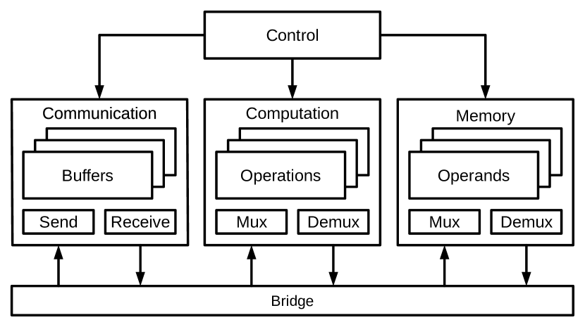
Figure 1: Division of the architecture into specialized modules.

Fig. 1 shows the division of the architecture into modules for communication, computation, memory, and control.

The communication module manages the exchange of data between the CPU and the FPGA. For this purpose, First-In First-Out (FIFO) buffers implemented in the on-chip Random Access Memory (RAM) of the FPGA are used. The transfer process itself is managed by a Direct Memory Access (DMA) controller on the low-level, and coordinated by a handshake protocol using interrupts on the high-level.

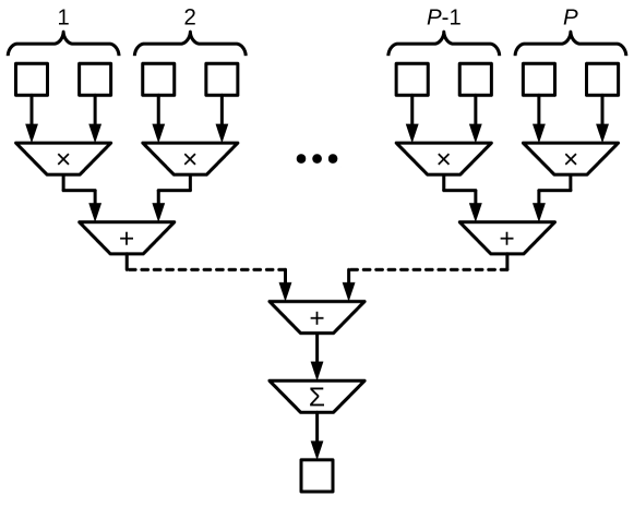
Figure 2: Parallelized implementation of the inner product.

The computation module comprises all resources for the actual calculations. According to Table X, the following operations are needed: (i) matrix addition / subtraction ($\boldsymbol{\mathbf{M}}_{1}\pm\boldsymbol{\mathbf{M}}_{2}$), (ii) vector addition / subtraction ($\boldsymbol{\mathbf{v}}_{1}\pm\boldsymbol{\mathbf{v}}_{2}$) and scaling ($s\cdot\boldsymbol{\mathbf{v}}$), (iii) the outer product ($\boldsymbol{\mathbf{v}}_{1}\boldsymbol{\mathbf{v}}_{2}^{T}$), (iv) the inner product ($\boldsymbol{\mathbf{v}}_{1}^{T}\boldsymbol{\mathbf{v}}_{2}$), and (v) the matrix-vector product ($\boldsymbol{\mathbf{M}}\boldsymbol{\mathbf{v}}$). In order to achieve high throughput, these operations are pipelined and parallized. Since parallel processing requires parallel data access, the operands need to be partitioned into blocks and stored in separate memories. Recall that the SDKF processes the measurements sequentially, so the parallelization is done with respect to the states. Say $P$ the degree of parallelization, then the matrix operands ($\boldsymbol{\mathbf{P}}_{k}^{-}$, $\boldsymbol{\mathbf{P}}_{k,i}^{+}$) are split into rasters of $P\times P$ blocks, and the vector operands ($\boldsymbol{\mathbf{H}}_{k,i}$, $\boldsymbol{\mathbf{C}}_{k,i}$, $\boldsymbol{\mathbf{K}}_{k,i}$, $\widehat{\boldsymbol{\mathbf{x}}}_{k}^{-}$, $\widehat{\boldsymbol{\mathbf{x}}}_{k,i}^{+}$) into arrays of $P$ blocks. Accordingly, the operations (i), (iii), and (v) are sped up by a factor of $P^{2}$, whereas (ii) and (iv) are accelerated by a factor of $P$. Of course, this requires the allocation of a corresponding number of arithmetic blocks. Note that the operations (i)–(iii) are straightforward to parallelize using arrays of adders or multipliers. The inner product (iv) can be built from a multiplier array, an adder tree, and one accumulator as depicted in Fig. 2. The matrix-vector product (v) is in turn made from $P$ replicas of (iv). For the synthesis of the arithmetic blocks, optimized libraries for Single-Precision Floating-Point (SGL) operations which exploit the Digital Signal Processing (DSP) slices of the FPGA to achieve high performance [39], are used. When configuring each block, a trade-off has to be made between throughput, latency, and resource consumption. For the RTSE application, high throughput and low resource consumption are crucial. The resulting configuration is listed in Table III.

TABLE III: Configuration of the arithmetic blocks

Operation	Throughput	Latency	DSPs
$\pm$	$1$ / cycle	$5$ cycles	$2$
$\times$	$1$ / cycle	$2$ cycles	$3$
$\sum$	$1$ / cycle	$20$ cycles	$9$
$\div$	$1$ / cycle	$20$ cylces	$8$

The memory module contains the storage for the operands. Note that one does not need to store all the intermediate results listed in Table X. Indeed, some of these operations are contracted in the FPGA implementation to increase the performance. Hence, it suffices to store $\boldsymbol{\mathbf{Q}}_{k}$, $\boldsymbol{\mathbf{R}}_{k}$, $\boldsymbol{\mathbf{H}}_{k}$, $\boldsymbol{\mathbf{z}}_{k}$, $\boldsymbol{\mathbf{C}}_{k,i}$, $\boldsymbol{\mathbf{K}}_{k,i}$, $\widehat{\boldsymbol{\mathbf{x}}}_{k}$ ($\widehat{\boldsymbol{\mathbf{x}}}_{k,i}^{+}$ / $\widehat{\boldsymbol{\mathbf{x}}}_{k}^{-}$), $\boldsymbol{\mathbf{P}}_{k}$ ($\boldsymbol{\mathbf{P}}_{k,i}^{+}$ / $\boldsymbol{\mathbf{P}}_{k}^{-}$), $\boldsymbol{\mathbf{W}}_{k,i}^{-1}$ and $\widehat{\boldsymbol{\mathbf{z}}}_{k,i}$. Recall from the above discussion that these operands are partitioned into blocks, which need to be stored in separate memories to allow for parallel processing. Therefore, one needs to take into consideration both the size and the organization of the available RAM when selecting the degree of parallelization $P$ for a given hardware platform. Firstly, there has to be enough memory (in terms of bits) to house the operands as a whole. Secondly, there need to be enough separate RAM slices for distributing the operands, which are divided into $P\times P$ or $P$ blocks, respectively.

TABLE IV: Resource occupation

Resource	Available	Occupied	Percentage
FFs	202’800	49’088	24.2
LUTs	101’400	43’166	42.6
DSPs	600	357	59.5
RAMs	325	262	80.6

With the FPGA resources available on the NI-cRIO-9033, the degree of parallelization that can be achieved with this architecture is $P=4$. Table IV lists the resource occupation in terms of Flip-Flops (FFs), Look-Up Tables (LUTs), DSPs, and RAMs obtained for this value of $P$. Clearly, the DSPs and the RAMs are the most critical resources. The high number of DSPs required is mainly due to the operations that require $P\times P$ arrays of arithmetic blocks, namely the matrix addition or subtraction (i), the outer product (iii), and the matrix-vector product (v). The high utilization of RAMs is mostly due to the operands $\boldsymbol{\mathbf{P}}_{k}$ and $\boldsymbol{\mathbf{H}}_{k}$, which are matrices whose number of elements is proportional to the square of the network size. The FFs and LUTs are principally used as shift registers for pipelining, but are obviously not critical resources.

IV-B Testbench

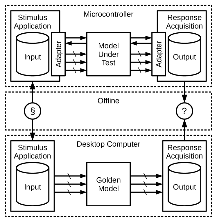
Figure 3: Schematic of the TB setup.

The TB setup depicted in Fig. 3 is used to validate the hardware implementation. It is divided into two separate parts associated to the MUT and the Golden Model (GM), which serves as the reference for the validation. The MUT part comprises the FPGA implementation of the SDKF along with some CPU software, and is executed on the NI-cRIO-9033, which runs NI Linux Real-Time and NI LabVIEW. The CPU software fulfills two purposes. Firstly, it coordinates the communication with the FPGA by handshaking, and steers the DMA controller that manages the data transfer. Secondly, it provides IO functionality for the TB files, namely reading the stimuli and writing the responses. In particular, there are protocol adapters which abstract the interface between the high-level data of the TB and the low-level data of the MUT. The GM part consists of a MATLAB implementation of the DKF, and is executed on a desktop machine under Mac OSX. Since the stimuli and the responses are stored in files, the MUT and the GM may be run independently. Therefore, the validation of the responses can be done offline.

V Experimental Validation

This section is dedicated to the validation of the developed hardware prototype. First, the results of the functional verification, which is based on test data for a benchmark distribution feeder, are presented in Section V-A. Then, the results of a scalability analysis, which is conducted using random data, are discussed in Section V-B.

V-A Functional Verification

TABLE V: Removed nodes

Type	Nodes (Naming according to [40])
Tie	802, 806, 808, 812, 818, 824, 854, 858, 834, 836

TABLE VI: Distributed generation and load

Type	Nodes (Naming according to [40])
DG	822, 856, 848, 838
DL	810, 816, 820, 826, 828, 832, 890, 864, 844, 860, 840

TABLE VII: PMU placement

Type	Nodes (Naming according to [40])
PMU	800, 806, 810, 816, 820, 822, 826, 828, 836
	832, 890, 864, 844, 848, 860, 840, 830

The benchmark system used for the functional verification is adapted from the IEEE 34-node distribution test feeder [40], which is an unbalanced three-phase grid with a rated line-to-line voltage of $24.9\,\text{kV}$ (RMS). The per unit base is chosen as $V_{b}=24.9\,\text{kV}$ and $S_{b}=1\,\text{MVA}$. For this work, the original configuration given in [40] is modified slightly by removing very short lines connected in series with very long ones (through merge). Note that the resulting reduced network is electrically equivalent to the original one, but does not consider some of its nodes with null injections (see Table V). The distribution feeder is connected to the feeding subtransmission grid in node 800. This link is characterized by a short-circuit power of $S_{sc}=300\,\text{MVA}$, and a short-circuit impedance $Z_{sc}$ with $R_{sc}/X_{sc}=0.1$. Furthermore, it is assumed that the voltage behind $Z_{sc}$ of the subtransmission system is constant, which implies that the corresponding feeding node behaves as an ideal slack. The lines are unbalanced and made from the same type of cable, so the per-unit-length resistance $\boldsymbol{\mathbf{R}}^{\prime}$, reactance $\boldsymbol{\mathbf{X}}^{\prime}$, and susceptance $\boldsymbol{\mathbf{B}}^{\prime}$ are identical for all lines. These parameters are listed in detail in [4]. Both generation and load are distributed across the entire feeder, as listed in Table VI. The profiles stem from a measurement campaign conducted on the EPFL campus in Lausanne, Switzerland [29]. Hence, the distributed load (DL) is a composition of offices and workshops, and the distributed generation (DG) are photovoltaic panels, which only inject active power.

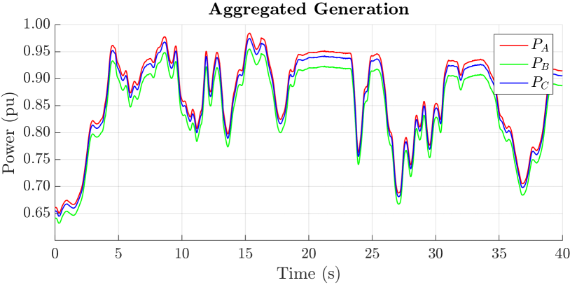
(a) Aggregated nodal injections (DG).

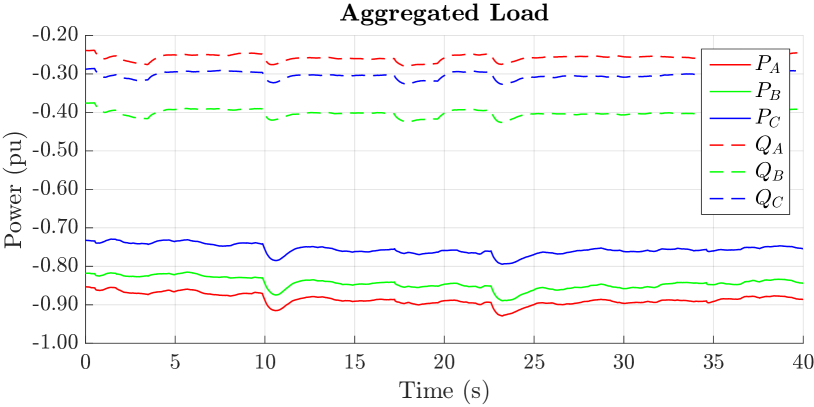
(b) Aggregated nodal absorptions (DL).

Figure 4: Aggregated power profiles.

See Fig. 4 for the aggregated profiles of power injection and absorption (generation is positive, load is negative). The PMUs are placed as given in Table VII so that the system is observable, which is ensured if $\boldsymbol{\mathbf{H}}_{k}$ has full rank [33]. Each PMU records the synchrophasors of nodal voltage and current in all phases at a refresh rate of 50 frames per second. The measurement system of the PMUs consists of class $0.1$ / $0.2$ voltage and current sensors (see [41, 42]).

1:procedure Measurements($\boldsymbol{\mathbf{S}}_{k}$, $\boldsymbol{\mathbf{Y}}_{k}$, $e_{\rho}$, $e_{\varphi}$)

2:     $\boldsymbol{\mathbf{V}}_{k}\leftarrow\textsc{LoadFlow}(\boldsymbol{\mathbf{S}}_{k},\boldsymbol{\mathbf{Y}}_{k})$

3:     $\widetilde{\boldsymbol{\mathbf{V}}}_{k}=\textsc{AddPolarNoise}(\boldsymbol{\mathbf{V}}_{k},e_{\rho},e_{\varphi})$

4:     $\boldsymbol{\mathbf{I}}_{k}=\boldsymbol{\mathbf{Y}}_{k}\boldsymbol{\mathbf{V}}_{k}$

5:     $\widetilde{\boldsymbol{\mathbf{I}}}_{k}=\textsc{AddPolarNoise}(\boldsymbol{\mathbf{I}}_{k},e_{\rho},e_{\varphi})$

6:     return $\boldsymbol{\mathbf{V}}_{k}$, $\widetilde{\boldsymbol{\mathbf{V}}}_{k}$, $\widetilde{\boldsymbol{\mathbf{I}}}_{k}$

7:end procedure

8:

9:procedure AddPolarNoise($\boldsymbol{\mathbf{x}}$, $e_{\rho}$, $e_{\varphi}$)

10:     $\sigma_{\rho}\leftarrow(1/3)\cdot e_{\rho}$

11:     $\sigma_{\varphi}\leftarrow(1/3)\cdot e_{\varphi}$

12:     for $i\in\{1,\ldots,\textsc{Length}(\boldsymbol{\mathbf{x}})\}$ do

13:         $\rho\leftarrow(1+\textsc{Gauss}(0,\sigma_{\rho}))\cdot|\boldsymbol{\mathbf{x}}(i)|$

14:         $\varphi\leftarrow(1+\textsc{Gauss}(0,\sigma_{\phi}))\cdot\angle(\boldsymbol{\mathbf{x}}(i))$

15:         $\widetilde{\boldsymbol{\mathbf{x}}}(i)\leftarrow\rho\angle\varphi$

16:     end for

17:     return $\widetilde{\boldsymbol{\mathbf{x}}}$

18:end procedure

Figure 5: Pseudocode describing the test data preparation.

To prepare the test data, the procedure in Fig. 5 is followed. The admittance matrix $\boldsymbol{\mathbf{Y}}_{k}$ and the nodal powers $\boldsymbol{\mathbf{S}}_{k}$ define a Load Flow (LF) problem at each time $k$, whose solution are the true nodal voltages $\boldsymbol{\mathbf{V}}_{k}$. In this respect, it is assumed that the topology of the network and the electrical parameters of the cables do not change during the considered period of time, so $\boldsymbol{\mathbf{Y_{k}}}=\boldsymbol{\mathbf{Y}}$ is constant. The measurement accuracy is determined by the metrological characteristics of the PMUs and their sensors. In practice, the impact of the sensors on the accuracy dominates. Thus, the measurements $\widetilde{\boldsymbol{\mathbf{V}}}_{k}$ and $\widetilde{\boldsymbol{\mathbf{I}}}_{k}$ may be obtained by perturbing the true values $\boldsymbol{\mathbf{V}}_{k}$ and $\boldsymbol{\mathbf{I}}_{k}$ with noise, whose distribution is determined by the sensor properties (see Fig. 5). For the used class $0.1$ / $0.2$ sensors, the inferred maximum errors are $e_{\rho}=10^{-3}~{}\text{pu}$ for magnitude and $e_{\varphi}=1.5\cdot 10^{-3}~{}\text{rad}$ for phase (see [5]). One may reasonably suppose that the sensor performance does not change with time, so $\boldsymbol{\mathbf{R}}_{k}=\boldsymbol{\mathbf{R}}$ is constant. Recall from Section III-A that $\boldsymbol{\mathbf{R}}$ models the measurement uncertainties in rectangular coordinates. The derivation of $\boldsymbol{\mathbf{R}}$ from the uncertainties in polar coordinates is explained in Appendix A.

As previously explained in Section III-B, there exist online assessment methods for $\boldsymbol{\mathbf{Q}}_{k}$, but they are beyond the scope of this paper. For the sake of brevity, the process noise covariance matrix is assumed to be a constant diagonal matrix $\boldsymbol{\mathbf{Q}}_{k}=\boldsymbol{\mathbf{Q}}$ with all diagonal entries set to $10^{-6}~{}\text{pu}^{2}$. Finally, the estimator needs initial values $\boldsymbol{\mathbf{P}}_{0}^{+}$ and $\widehat{\boldsymbol{\mathbf{x}}}_{0}^{+}$. One can use $\boldsymbol{\mathbf{P}}_{0}^{+}=\boldsymbol{\mathbf{Q}}$, and set $\widehat{\boldsymbol{\mathbf{x}}}_{0}^{+}$ to a flat voltage profile. Then, the responses $\widehat{\boldsymbol{\mathbf{x}}}_{k}^{+}|_{\text{GM}}$ and $\widehat{\boldsymbol{\mathbf{x}}}_{k}^{+}|_{\text{MUT}}$, i.e. the estimated state $\widehat{\boldsymbol{\mathbf{x}}}_{k}^{+}$ provided by the GM and the MUT, are recorded in the TB setup. The corresponding estimated nodal voltage phasors $\widehat{\boldsymbol{\mathbf{V}}}_{k}|_{\text{MUT}}$ and $\widehat{\boldsymbol{\mathbf{V}}}_{k}|_{\text{GM}}$ are defined by (4).

For the validation, one needs to look at the estimation accuracy and the numerical accuracy. The former is related to the estimation error $\widehat{\boldsymbol{\mathbf{V}}}_{k}-\boldsymbol{\mathbf{V}}_{k}$, where $\widehat{\boldsymbol{\mathbf{V}}}_{k}$ is a placeholder for $\widehat{\boldsymbol{\mathbf{V}}}_{k}|_{\text{MUT}}$ and $\widehat{\boldsymbol{\mathbf{V}}}_{k}|_{\text{GM}}$. The latter corresponds to the mismatch $\widehat{\boldsymbol{\mathbf{V}}}_{k}|_{\text{MUT}}-\widehat{\boldsymbol{\mathbf{V}}}_{k}|_{\text{GM}}$. To be more precise, one is interested in the statistical distribution of these quantities. For this analysis, the true voltages $V_{b,p,k}$ and the estimated voltages $\widehat{V}_{b,p,k}$ are expressed in polar coordinates. That is

$$V_{b,p,k} =|V_{b,p,k}|\angle\delta_{b,p,k}$$ (70)

$$\widehat{V}_{b,p,k} =|\widehat{V}_{b,p,k}|\angle\widehat{\delta}_{b,p,k}$$ (71)

Recall that $b\in\mathcal{B}$ is the bus, and $p\in\mathcal{P}$ is the phase.

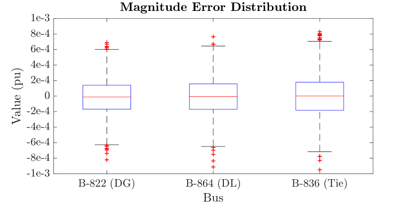
(a) Magnitude error $|\widehat{V}_{b,p,k}|-|V_{b,p,k}|$.

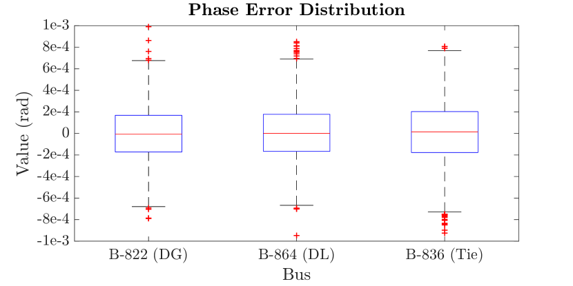
(b) Phase error $\widehat{\delta}_{b,p,k}-\delta_{b,p,k}$.

Figure 6: Distribution of the error $\widehat{V}_{b,p,k}-V_{b,p,k}$.

(a) Magnitude mismatch $|\widehat{V}_{b,p,k}|_{\text{MUT}}-|\widehat{V}_{b,p,k}|_{\text{GM}}$.

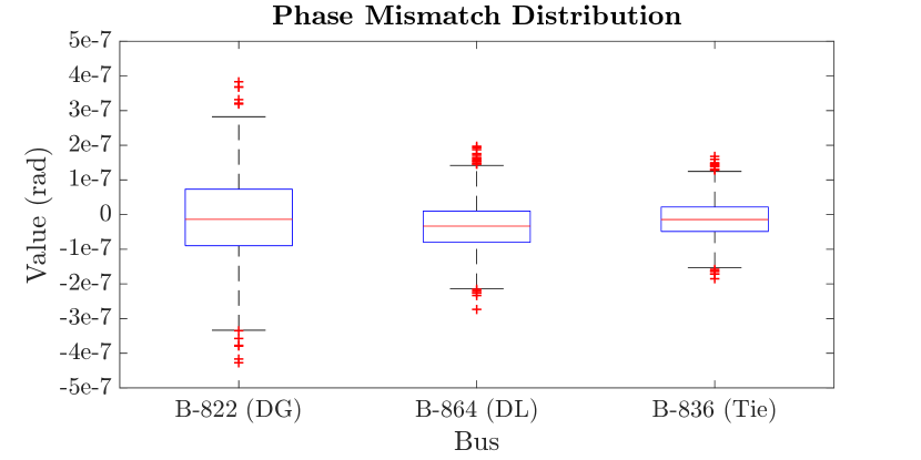
(b) Phase mismatch $\widehat{\delta}_{b,p,k}|_{\text{MUT}}-\widehat{\delta}_{b,p,k}|_{\text{GM}}$.

Figure 7: Distribution of the mismatch $\widehat{V}_{b,p,k}|_{\text{MUT}}-\widehat{V}_{b,p,k}|_{\text{GM}}$.

It has been verified that the distribution of the error and mismatch quantities are static and close to normal, which is in accordance with the assumptions made for the persistence process model (6) and the measurement model (9). The resulting distributions of the error and the mismatch are visualized in Fig. 6 and Fig. 7 for three different buses. The sample data correspond to a time window of $40$ seconds (i.e. $2000$ samples at $50$ frames per second). As one can see in Fig. 6, the estimation error is low both in magnitude and phase: half of the samples are within $\pm 2\cdot 10^{-4}$ (pu / rad). This indicates that the SDKF is tracking the state correctly, and is in accordance with the performance assessment in [5]. As Fig. 7 reveals, the results of the MUT match well with those of the GM. Even at the bus with the largest mismatch, the magnitude and phase mismatch are within $\pm 1\cdot 10^{-6}\text{pu}$ and $\pm 5\cdot 10^{-7}\text{rad}$, respectively. Since the mismatch is substantially smaller than the modeled uncertainties, it can be concluded that the inaccuracy due to the use of SGL precision on the FPGA, as compared to DBL precision on the CPU, is negligible. In fact, since SGL precision provides an accuracy of 6–7 decimal digits, and a mismatch of $\leqslant 10^{-6}$ is expected. Therefore, it can be concluded that the MUT is equivalent to the GM within the bounds of the numerical accuracy.

V-B Scalability Analysis

To assess the scalability of the RTSE, the execution time of the FPGA is measured for estimation problems of different size. Since benchmark feeders of arbitrary size are not readily available, the necessary data are randomly generated, while ensuring that the working hypotheses of the SDKF hold. For simplicity, it is assumed that $D=S$, so an actual system would be observable with no redundancy. The problem size is essentially limited by the amount of memory available on the FPGA, namely $S<256$ if $D=S$. Assuming an unreduced three-phase network, this corresponds to $N=255/(3\cdot 2)\approx 42$ nodes. If network reduction techniques are used, for example the elimination of tie buses (applicable for any kind of network) or the use of the single-phase equivalent (balanced networks only), considerably larger networks can be accommodated. Note that execution time is defined as the time passing between the reading of the input and the writing of the output on the FPGA. In order to measure this time as accurately as possible, a counter driven by the master clock is implemented directly on the chip. As the frequency of the master clock is known precisely, it is straightforward to derive the time from the counter state.

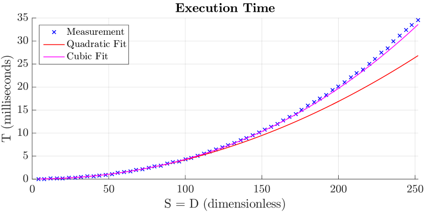
Figure 8: Execution time.

The obtained results are shown in Fig. 8. As one can see, the time required for the largest problem size is 35 ms. In order to visualize the time complexity, a quadratic and a cubic curve are fit to the portion of the curve for which $S\leqslant 80$. As one would expect from the computational complexity analysis presented in Section III-E, the time scales with the third power of the problem size. However, it is worth noticing that the third order term is not dominant for this range of problem sizes, since the cubic fit is not too far from the quadratic one. This effect is due to the combination of parallelization and pipelining adopted for the implementation, as described in Section IV-A. For small problem sizes, the execution of the linear algebra blocks is dominated by the latency (the pipeline depth) rather than the number of items to be processed.

VI Conclusion

This paper has presented an FPGA prototype of an RTSE for ADNs based on the SDKF. To motivate the use of the SDKF rather than the DKF, it has been proven that the two formulations are formally equivalent (for uncorrelated measurement noise), and demonstrated that only the SDKF is suitable for an implementation in this dedicated hardware. To this effect, it has also been illustrated that the SDKF only involves elementary linear algebra operations, which can be parallelized and pipelined in order to achieve high throughput. The obtained results confirm that the developed FPGA implementation of the SDKF yields the same results as the reference CPU implementation of the DKF, while guaranteeing real-time performance. In particular, the use of the SGL number format on the FPGA as opposed to the DBL number format on the CPU does not cause any noteworthy inaccuracy. Therefore, it can be concluded that RTSEs on the basis of dedicated hardware implementations are indeed feasible, and may hence support the development of automation systems for ADNs.

Appendix A Transformation of the Uncertainty
from Polar to Rectangular Coordinates

Say $V=|V|\angle\delta$ the true value of a voltage phasor in polar coordinates. Let $\Delta|V|$ and $\Delta\delta$ be the associated measurement errors, so that the measured phasor $\widetilde{V}$ may be written as

$$\widetilde{V}=(|V|+\Delta|V|)\angle(\delta+\Delta\delta)$$ (72)

where $\Delta|V|$ and $\Delta\delta$ are assumed to be normally distributed

$$\Delta|V| \sim\mathcal{N}(0,\sigma_{m}^{2})$$ (73)

$$\Delta\delta \sim\mathcal{N}(0,\sigma_{p}^{2})$$ (74)

According to Euler’s Formula $\widetilde{V}=\widetilde{V}_{r}+j\widetilde{V}_{i}$

$$\widetilde{V}_{r} =(|V|+\Delta|V|)\cos(\delta+\Delta\delta)=V_{r}+\Delta V_{r}$$ (75)

$$\widetilde{V}_{i} =(|V|+\Delta|V|)\sin(\delta+\Delta\delta)=V_{i}+\Delta V_{i}$$ (76)

where $\Delta V_{r}$ and $\Delta V_{i}$ are the measurement errors in rectangular coordinates. If $\Delta|V|$ and $\Delta\delta$ are independent, the variances $\sigma_{r}^{2}$ and $\sigma_{i}^{2}$ of $\Delta V_{r}$ and $\Delta V_{i}$ are given by [4]

$$\sigma_{r}^{2} =\left\{\begin{aligned} |V|^{2}e^{-\sigma_{p}^{2}}&\left[\cos^{2}\delta(\cosh^{2}(\sigma_{p}^{2})-1)+\sin^{2}\delta\sinh^{2}(\sigma_{p}^{2})\right]\\ +\sigma_{m}^{2}e^{-\sigma_{p}^{2}}&\left[\cos^{2}\delta\cosh^{2}(\sigma_{p}^{2})+\sin^{2}\delta\sinh^{2}(\sigma_{p}^{2})\right]\end{aligned}\right.$$ (77)

$$\sigma_{i}^{2} =\left\{\begin{aligned} |V|^{2}e^{-\sigma_{p}^{2}}&\left[\sin^{2}\delta(\cosh^{2}(\sigma_{p}^{2})-1)+\cos^{2}\delta\sinh^{2}(\sigma_{p}^{2})\right]\\ +\sigma_{m}^{2}e^{-\sigma_{p}^{2}}&\left[\sin^{2}\delta\cosh^{2}(\sigma_{p}^{2})+\cos^{2}\delta\sinh^{2}(\sigma_{p}^{2})\right]\end{aligned}\right.$$ (78)

Evidently, the uncertainties $\sigma_{r}$ and $\sigma_{i}$ in the rectangular coordinate system do not only depend on the corresponding $\sigma_{m}$ and $\sigma_{p}$ in the polar coordinate system, but also on the true magnitude and phase $|V|$ and $\delta$, which are unknown in practice. Consider the case of the functional verification in Section V-A. A maximum measurement error of $1\cdot 10^{-3}\text{pu}$ in magnitude and $1.5\cdot 10^{-3}\text{rad}$ in phase implies

$$\sigma_{m} \approx 3^{-1}\cdot 10^{-3}~{}\text{pu}$$ (79)

$$\sigma_{p} \approx 5\cdot 10^{-4}~{}\text{rad}$$ (80)

Table VIII lists $\sigma_{r}$ and $\sigma_{i}$ computed for $|V|=1~{}\text{pu}$ and different phase angles $\delta\in[0,\pi]~{}\text{rad}$. According to (4), (14), and Hypothesis 3, $\sigma_{r}^{2}$ and $\sigma_{i}^{2}$ appear on the diagonal of $\boldsymbol{\mathbf{R}}_{k}$. If desired, $\boldsymbol{\mathbf{R}}_{k}$ can thus be updated online based on the received measurements using the projection defined by (77) and (78). In this work, $\boldsymbol{\mathbf{R}}_{k}=\boldsymbol{\mathbf{R}}$ is presumed constant for the sake of simplicity (see Section V-A). For the transformation of $\sigma_{m}$ and $\sigma_{p}$ to $\sigma_{r}$ and $\sigma_{i}$, it is assumed that the system is balanced, and that both the voltage drop and the phase angle difference of any bus with respect to the slack are small. That is, $\forall b\in\mathcal{B}$

$$|V_{b,1}|=|V_{b,1}|=|V_{b,1}|\approx 1~{}\text{pu}$$ (81)

$$\delta_{b,1}\approx 0~{}\text{rad},~{}\delta_{b,2}\approx-\frac{2\pi}{3}~{}\text{rad},~{}\delta_{b,3}\approx+\frac{2\pi}{3}~{}\text{rad}$$ (82)

TABLE VIII: Numerical example

$|V|$ (pu)	$\delta~{}(\text{rad})$	$\sigma_{r}$ (pu)	$\sigma_{i}~{}(\text{pu})$
1	$0$	$3.333\cdot 10^{-4}$	$5.000\cdot 10^{-4}$
1	$\pm\frac{\pi}{6}$	$3.819\cdot 10^{-4}$	$4.640\cdot 10^{-4}$
1	$\pm\frac{\pi}{3}$	$4.640\cdot 10^{-4}$	$3.819\cdot 10^{-4}$
1	$\pm\frac{\pi}{2}$	$5.000\cdot 10^{-4}$	$3.333\cdot 10^{-4}$
1	$\pm\frac{2\pi}{3}$	$4.640\cdot 10^{-4}$	$3.819\cdot 10^{-4}$
1	$\pm\frac{5\pi}{6}$	$3.819\cdot 10^{-4}$	$4.640\cdot 10^{-4}$
1	$\pi$	$3.333\cdot 10^{-4}$	$5.000\cdot 10^{-4}$

Appendix B Strict Positive Definiteness
of the Estimation Error Covariance

If the estimation error covariance matrix is initialized to be positive definite at start-up ($\boldsymbol{\mathbf{P}}_{0}^{+}\succ 0$), $\boldsymbol{\mathbf{P}}_{k}^{-}$ and $\boldsymbol{\mathbf{P}}_{k}^{+}$ will remain positive definite for $k\geqslant 1$, because this property is preserved by the operations of the DKF. For the prediction step, this is straightforward to show. From (24), it is easy to see that

$$\boldsymbol{\mathbf{P}}_{k-1}^{+}\succ 0,~{}\boldsymbol{\mathbf{Q}}_{k}\succeq 0\quad\Longrightarrow\quad\boldsymbol{\mathbf{P}}_{k}^{-}=\boldsymbol{\mathbf{P}}_{k-1}^{+}+\boldsymbol{\mathbf{Q}}_{k}\succ 0$$ (83)

For the estimation step, the following Lemma will be used.

Lemma 3.

If $\boldsymbol{\mathbf{A}}$ is a positive (semi)definite matrix, and $\boldsymbol{\mathbf{B}}$ is an arbitrary matrix with full rank, then the matrix $\boldsymbol{\mathbf{C}}=\boldsymbol{\mathbf{B}}^{T}\boldsymbol{\mathbf{A}}\boldsymbol{\mathbf{B}}$ is also positive (semi)definite.

Consider first the formulation (25)–(27) of the estimation step. It should be noted that (27) is actually a simplified version of a more complex symmetric expression, namely [34]

$$\boldsymbol{\mathbf{P}}_{k}^{+} =(\boldsymbol{\mathbf{I}}-\boldsymbol{\mathbf{K}}_{k}\boldsymbol{\mathbf{H}}_{k})\boldsymbol{\mathbf{P}}_{k}^{-}$$ (84)

$$=(\boldsymbol{\mathbf{I}}-\boldsymbol{\mathbf{K}}_{k}\boldsymbol{\mathbf{H}}_{k})\boldsymbol{\mathbf{P}}_{k}^{-}(\boldsymbol{\mathbf{I}}-\boldsymbol{\mathbf{K}}_{k}\boldsymbol{\mathbf{H}}_{k})^{T}+\boldsymbol{\mathbf{K}}_{k}\boldsymbol{\mathbf{R}}_{k}\boldsymbol{\mathbf{K}}_{k}^{T}$$ (85)

Recall from (25) that $\boldsymbol{\mathbf{K}}_{k}$ is given by

$$\boldsymbol{\mathbf{K}}_{k}=\boldsymbol{\mathbf{P}}_{k}^{-}\boldsymbol{\mathbf{H}}_{k}^{T}(\boldsymbol{\mathbf{H}}_{k}\boldsymbol{\mathbf{P}}_{k}^{-}\boldsymbol{\mathbf{H}}_{k}^{T}+\boldsymbol{\mathbf{R}}_{k})^{-1}$$ (86)

Since $\boldsymbol{\mathbf{H}}_{k}$ has full rank (Hypothesis 1), $\boldsymbol{\mathbf{R}}_{k}$ is positive semidefinite by definition, and $\boldsymbol{\mathbf{P}}_{k}^{-}$ is positive definite by assumption, it follows that $(\ldots)^{-1}$ exists and that $\boldsymbol{\mathbf{K}}_{k}$ has full rank. By application of Lemma 3 to (85), it follows that $\boldsymbol{\mathbf{P}}_{k}^{+}$ is positive definite. Consider now the formulation (28)–(30) of the estimation step, which states that

$$(\boldsymbol{\mathbf{P}}_{k}^{+})^{-1}=(\boldsymbol{\mathbf{P}}_{k}^{-})^{-1}+\boldsymbol{\mathbf{H}}_{k}^{T}\boldsymbol{\mathbf{R}}_{k}^{-1}\boldsymbol{\mathbf{H}}_{k}$$ (87)

If $(\boldsymbol{\mathbf{P}}_{k}^{-})$ is positive definite, its inverse exists and is positive definite as well. The term $\boldsymbol{\mathbf{H}}_{k}^{T}\boldsymbol{\mathbf{R}}_{k}^{-1}\boldsymbol{\mathbf{H}}_{k}$ is positive definite according to Lemma 3. By consequence, the sum term that defines $(\boldsymbol{\mathbf{P}}_{k}^{+})^{-1}$ is positive definite.

As the prediction step and the estimation step preserve the positive definiteness of $\boldsymbol{\mathbf{P}}_{k}^{-}$ and $\boldsymbol{\mathbf{P}}_{k}^{+}$ after an initialization with corresponding values, Hypothesis 2 is indeed reasonable.

Appendix C Discrete Kalman Filter Complexity

Table IX and Table X list the number of operations required for each step of the DKF and the SDKF, respectively.

TABLE IX: Detailed Computational Complexity (DKF)

Prediction Step		$+|-$	$\times|\div$
$\widehat{\boldsymbol{\mathbf{x}}}_{k}^{-}$	${}=\widehat{\boldsymbol{\mathbf{x}}}_{k-1}^{+}$	$0$	$0$
$\boldsymbol{\mathbf{P}}_{k}^{-}$	${}=\boldsymbol{\mathbf{P}}_{k-1}^{-}+\boldsymbol{\mathbf{Q}}_{k}$	$S$	$0$
Estimation Step		$+|-$	$\times|\div$
Reusable Coefficient
$\boldsymbol{\mathbf{C}}_{k}$	${}=\boldsymbol{\mathbf{H}}_{k}\boldsymbol{\mathbf{P}}_{k}^{-}$	$DS(S-1)$	$DS^{2}$
Kalman Gain
$d\boldsymbol{\mathbf{R}}_{k}$	${}=\boldsymbol{\mathbf{C}}_{k}\boldsymbol{\mathbf{H}}_{k}^{T}$	$D^{2}(S-1)$	$D^{2}S$
$\boldsymbol{\mathbf{W}}_{k}$	${}=\boldsymbol{\mathbf{R}}_{k}+d\boldsymbol{\mathbf{R}}_{k}$	$D$	$0$
	${}\boldsymbol{\mathbf{W}}_{k}^{-1}$	$m\in\mathcal{O}(D^{3})$	$n\in\mathcal{O}(D^{3})$
$\boldsymbol{\mathbf{K}}_{k}$	${}=\boldsymbol{\mathbf{C}}_{k}^{T}\boldsymbol{\mathbf{W}}_{k}^{-1}$	$D(D-1)S$	$D^{2}S$
Estimated State
$\widehat{\boldsymbol{\mathbf{z}}}_{k}$	${}=\boldsymbol{\mathbf{H}}_{k}\widehat{\boldsymbol{\mathbf{x}}}_{k}^{-}$	$D(S-1)$	$DS$
$d\boldsymbol{\mathbf{z}}_{k}$	${}=\boldsymbol{\mathbf{z}}_{k}-\widehat{\boldsymbol{\mathbf{z}}}_{k}$	$D$	$0$
$d\boldsymbol{\mathbf{x}}_{k}$	${}=\boldsymbol{\mathbf{K}}_{k}d\boldsymbol{\mathbf{z}}_{k}$	$(D-1)S$	$DS$
$\widehat{\boldsymbol{\mathbf{x}}}_{k}^{+}$	${}=\widehat{\boldsymbol{\mathbf{x}}}_{k}^{-}+d\boldsymbol{\mathbf{x}}_{k}$	$S$	$0$
Estimation Error Covariance
$d\boldsymbol{\mathbf{P}}_{k}$	${}=\boldsymbol{\mathbf{K}}_{k}\boldsymbol{\mathbf{C}}_{k}$	$(D-1)S^{2}$	$DS^{2}$
$\boldsymbol{\mathbf{P}}_{k}^{+}$	${}=\boldsymbol{\mathbf{P}}_{k}^{-}-d\boldsymbol{\mathbf{P}}_{k}$	$S^{2}$	$0$

TABLE X: Detailed Computational Complexity (SDKF)

Prediction Step		$+|-$	$\times|\div$
$\widehat{\boldsymbol{\mathbf{x}}}_{k}^{-}$	${}=\widehat{\boldsymbol{\mathbf{x}}}_{k-1}$	$0$	$0$
$\boldsymbol{\mathbf{P}}_{k}^{-}$	${}=\boldsymbol{\mathbf{P}}_{k-1}^{+}+\boldsymbol{\mathbf{Q}}{k}$	$S$	$0$
Estimation Step		$+|-$	$\times|\div$
FOR $i\in\{1,\ldots,D\}$
Reusable Coefficient
$\boldsymbol{\mathbf{C}}_{k,i}$	${}=\boldsymbol{\mathbf{H}}_{k,i}\boldsymbol{\mathbf{P}}_{k,i-1}^{+}$	$S(S-1)$	$S^{2}$
Kalman Gain
$d\boldsymbol{\mathbf{R}}_{k,i}$	${}=\boldsymbol{\mathbf{C}}_{k,i}\boldsymbol{\mathbf{H}}_{k,i}^{T}$	$S-1$	$S$
$\boldsymbol{\mathbf{W}}_{k,i}$	${}=\boldsymbol{\mathbf{R}}_{k,i}+d\boldsymbol{\mathbf{R}}_{k,i}$	$1$	$0$
	${}\boldsymbol{\mathbf{W}}_{k,i}^{-1}$	$0$	$1$
$\boldsymbol{\mathbf{K}}_{k,i}$	${}=\boldsymbol{\mathbf{C}}_{k,i}^{T}\boldsymbol{\mathbf{W}}_{k,i}^{-1}$	$0$	$S$
Estimated State
$\widehat{\boldsymbol{\mathbf{z}}}_{k,i}$	${}=\boldsymbol{\mathbf{H}}_{k,i}\widehat{\boldsymbol{\mathbf{x}}}_{k,i-1}^{+}$	$S-1$	$S$
$d\boldsymbol{\mathbf{z}}_{k,i}$	${}=\boldsymbol{\mathbf{z}}_{k,i}-\widehat{\boldsymbol{\mathbf{z}}}_{k,i}$	$1$	$0$
$d\boldsymbol{\mathbf{x}}_{k,i}$	${}=\boldsymbol{\mathbf{K}}_{k,i}d\boldsymbol{\mathbf{z}}_{k,i}$	$0$	$S$
$\widehat{\boldsymbol{\mathbf{x}}}_{k,i}^{+}$	${}=\widehat{\boldsymbol{\mathbf{x}}}_{k,i-1}^{+}+d\boldsymbol{\mathbf{x}}_{k,i}$	$S$	$0$
Estimation Error Covariance
$d\boldsymbol{\mathbf{P}}_{k,i}$	${}=\boldsymbol{\mathbf{K}}_{k,i}\boldsymbol{\mathbf{C}}_{k,i}$	$0$	$S^{2}$
$\boldsymbol{\mathbf{P}}_{k,i}^{+}$	${}=\boldsymbol{\mathbf{P}}_{k,i-1}^{+}-d\boldsymbol{\mathbf{P}}_{k}$	$S^{2}$	$0$
END

Andreas Martin Kettner (M’15) grew up in Sünikon, Switzerland, and attended the Kantonsschule Zürcher Unterland in Bülach, Switzerland. He received the B.Sc. and M.Sc. degrees in Electrical Engineering and Information Technology from the Eidgenössische Technische Hochschule Zürich, Switzerland, in 2012 and 2014, respectively. After working as a development engineer for Supercomputing Systems AG in Zürich, he joined the Distributed Electrical Systems Laboratory at the École Polytechnique Fédérale de Lausanne, Switzerland, where he is pursuing a Ph.D. degree. His research interests include real-time monitoring and control of Active Distribution Networks with particular focus on State Estimation and Voltage Stability Assessment.

Mario Paolone (M’07–SM’10) received the M.Sc. (Hons.) and Ph.D. degrees in electrical engineering from the University of Bologna, Bologna, Italy, in 1998 and 2002, respectively. In 2005, he was nominated Assistant Professor in power systems at the University of Bologna, where he was with the power systems laboratory until 2011. He is currently an Associate Professor at the Swiss Federal Institute of Technology, Lausanne, Switzerland, chair of the Distributed Electrical Systems Laboratory. He was the Co-Chairperson of the Technical Committee of the 9th edition of the International Conference of Power Systems Transients (2009) and of the 19th and 20th Power Systems Computation Conference (2016 and 2018). He is author or coauthor of more than 220 scientific papers published in reviewed journals and international conferences. He is the Editor-in-Chief of the Elsevier journal Sustainable Energy, Grids and Networks and the Head of the Swiss Competence Center for Energy Research “FURIES”. His research interests include power systems with particular reference to real-time monitoring and operation of active distribution networks, integration of distributed energy storage systems, power system protections and power system transients. In 2013, he received the IEEE EMC Society Technical Achievement Award.

References

- [1] “IEEE Standard for Synchrophasor Measurements for Power Systems,” 2011, IEEE Standard C37.118.1.
- [2] “IEEE Standard for Synchrophasor Data Transfer for Power Systems,” 2011, IEEE Standard C37.118.2.
- [3] P. Romano and M. Paolone, “Enhanced Interpolated-DFT for Synchrophasor Estimation in FPGAs: Theory, Implementation, and Validation of a PMU Prototype,” IEEE Trans. Instrum. Meas., vol. 63, no. 12, pp. 2824–2836, May 2014.
- [4] M. Paolone, J.-Y. Le Boudec, S. Sarri, and L. Zanni, “Static and Recursive PMU-based State Estimation Processes for Transmission and Distribution Grids,” in Advanced Techniques for Power System Modelling, Control and Stability Analysis, F. Milano, Ed. Stevenage, HRT, UK: IET, 2016.
- [5] S. Sarri, L. Zanni, M. Popovic, J.-Y. Le Boudec, and M. Paolone, “Performance Assessment of Linear State Estimators using Synchrophasor Measurements,” IEEE Trans. Instrum. Meas., vol. 65, no. 3, pp. 535–548, March 2016.
- [6] F. F. Wu, K. Moslehi, and A. Bose, “Power System Control Centers: Past, Present, and Future,” Proc. IEEE, vol. 93, no. 11, pp. 1890–1908, October 2005.
- [7] F. C. Schweppe and J. Wildes, “Power System Static-State Estimation, Part I: Exact Model,” IEEE Trans. Power App. Syst., no. 1, pp. 120–125, January 1970.
- [8] F. C. Schweppe and D. B. Rom, “Power System Static-State Estimation, Part II: Approximate Model,” IEEE Trans. Power App. Syst., no. 1, pp. 125–130, January 1970.
- [9] F. C. Schweppe, “Power System Static-State Estimation, Part III: Implementation,” IEEE Trans. Power App. Syst., no. 1, pp. 130–135, January 1970.
- [10] J. J. Grainger and W. D. Stevenson, Power System Analysis. New York City, NY, USA: McGraw-Hill Education, 1994.
- [11] A. J. Monticelli, State Estimation in Electric Power Systems: A Generalized Approach. Berlin, Germany: Springer Science & Business Media, 1999.
- [12] A. Abur and A. Gómez Expósito, Power System State Estimation: Theory and Implementation. Boca Ranton, FL, USA: CRC Press, 2004.
- [13] F. C. Schweppe and E. J. Handschin, “Static State Estimation in Electric Power Systems,” Proc. IEEE, vol. 62, no. 7, pp. 972–982, July 1974.
- [14] A. J. Monticelli, “Electric Power System State Estimation,” Proc. IEEE, vol. 88, no. 2, pp. 262–282, February 2000.
- [15] A. Gómez-Expósito, A. de la Villa Jaén, C. Gómez-Quiles, P. Rousseaux, and T. Van Cutsem, “A Taxonomy of Multi-Area State Estimation Methods,” Electric Power Systems Research, vol. 81, no. 4, pp. 1060–1069, April 2011.
- [16] Y. Liu, W. Jiang, S. Jin, M. Rice, and Y. Chen, “Distributing Power Grid State Estimation on HPC Clusters - A System Architecture Prototype,” in IEEE International Parallel & Distributed Processing Symposium (IPDPS), Shanghai, China, May 2012, pp. 1467–1476.
- [17] S. K. Khaitan and A. Gupta, Eds., High Performance Computing in Power and Energy Systems. Berlin, Germany: Springer Science & Business Media, 2013.
- [18] G. N. Korres, A. Tzavellas, and E. Galinas, “A Distributed Implementation of Multi-Area Power System State Estimation on a Cluster of Computers,” Electric Power Systems Research, vol. 102, pp. 20–32, September 2013.
- [19] H. Karimipour and V. Dinavahi, “Accelerated Parallel WLS State Estimation for Large-Scale Power Systems on GPU,” in North American Power Symposium (NAPS), Manhattan, KS, USA, 2013, pp. 1–6.
- [20] N. Hatziargyriou, J. Amantegui, B. Andersen, M. Armstrong, P. Boss, B. Dalle, G. De Montravel, A. Negri, C. A. Nucci, and P. Southwell, “Electricity Supply Systems of the Future,” Electra, no. 256, pp. 42–49, May 2011.
- [21] CIGRÉ Task Force C6.11, “Development and Operation of Active Distribution Networks,” CIGRÉ, Paris, France, Tech. Rep. 457, 2011.
- [22] J. Liu, J. Tang, F. Ponci, A. Monti, C. Muscas, and P. A. Pegoraro, “Trade-Offs in PMU Deployment for State Estimation in Active Distribution Grids,” IEEE Trans. Smart Grid, vol. 3, no. 2, pp. 915–924, June 2012.
- [23] C. Lu, J. Teng, and W.-H. Liu, “Distribution System State Estimation,” IEEE Trans. Power Syst., vol. 10, no. 1, pp. 229–240, February 1995.
- [24] D. A. Haughton and G. T. Heydt, “A Linear State Estimation Formulation for Smart Distribution Systems,” IEEE Trans. Power Syst., vol. 28, no. 2, pp. 1187–1195, May 2013.
- [25] M. E. Baran and A. W. Kelley, “A Branch-Current-Based State Estimation Method for Distribution Systems,” IEEE Trans. Power Syst., vol. 10, pp. 483–491, February 1995.
- [26] A. S. Debs and R. E. Larson, “A Dynamic Estimator for Tracking the State of a Power System,” IEEE Trans. Power App. Syst., no. 7, pp. 1670–1678, September 1970.
- [27] L. Zanni, S. Sarri, M. Pignati, R. Cherkaoui, and M. Paolone, “Probabilistic Assessment of the Process-Noise Covariance Matrix of Discrete Kalman Filter State Estimation of Active Distribution Networks,” in International Conference on Probabilistic Methods Applied to Power Systems (PMAPS), Durham, DUR, UK, 2014, pp. 1–6.
- [28] L. Zanni, J.-Y. Le Boudec, R. Cherkaoui, and M. Paolone, “A Prediction-Error Covariance Estimator for Adaptive Kalman Filtering in Step-Varying Processes: Application to Power-System State Estimation,” IEEE Trans. Control Syst. Technol., vol. PP, no. 99, pp. 1–15, December 2016.
- [29] M. Pignati, M. Popovic, S. Barreto, R. Cherkaoui, G. D. Flores, J.-Y. Le Boudec, M. Mohiuddin, M. Paolone, P. Romano, S. Sarri et al., “Real-Time State Estimation of the EPFL-Campus Medium-Voltage Grid by using PMUs,” in IEEE PES Innovative Smart Grid Technologies Conference (ISGT), Washington, DC, USA, 2015, pp. 1–5.
- [30] J. Arrillaga and C. P. Arnold, Computer Analysis of Power Systems. Hoboken, NJ, USA: John Wiley & Sons, 1990.
- [31] R. E. Kalman, “A New Approach to Linear Filtering and Prediction Problems,” Journal of Basic Engineering, vol. 82, no. 1, pp. 35–45, 1960.
- [32] D. Belega and D. Petri, “Accuracy Analysis of the Multicycle Synchrophasor Estimator Provided by the Interpolated DFT Algorithm,” IEEE Trans. Instrum Meas., vol. 62, no. 5, pp. 942–953, May 2013.
- [33] N. M. Manousakis, G. N. Korres, and P. S. Georgilakis, “Taxonomy of PMU Placement Methodologies,” IEEE Trans. Power Syst., vol. 27, no. 2, pp. 1070–1077, May 2012.
- [34] D. Simon, Optimal State Estimation: Kalman, , and Nonlinear Approaches. Hoboken, NJ, USA: John Wiley & Sons, 2006.
- [35] S. Sarri, “Methods and Performance Assessment of PMU-based Real-Time State Estimation of Active Distribution Networks,” Dissertation, École Polytechnique Fédérale de Lausanne, Faculté Sciences et Techniques de l’Ingénieur, Lausanne, VD, CH, 2016.
- [36] R. G. Brown and P. Y. C. Hwang, Introduction to Random Signals and Applied Kalman Filtering, 4th ed. Hoboken, NJ, USA: John Wiley & Sons, 2012.
- [37] C. Muscas, M. Pau, P. A. Pegoraro, and S. Sulis, “Effects of Measurements and Pseudomeasurements Correlation in Distribution System State Estimation,” IEEE Trans. Instrum Meas., vol. 63, no. 12, pp. 2813–2823, December 2014.
- [38] NI cRIO-9033 Operating Instructions and Specifications, National Instruments Corporation, Austin, TX, USA, August 2014.
- [39] 7 Series DSP48E1 Slice User Guide, Xilinx Inc., San José, CA, USA, September 2016, UG 479 (Version 1.9).
- [40] W. H. Kersting, “Radial Distribution Test Feeders,” IEEE Trans. Power Syst., vol. 6, no. 3, pp. 975–985, August 1991.
- [41] “Instrument Transformers - Part 1: General Requirements,” 2010, IEC Standard 61869-1.
- [42] “Instrument Transformers - Part 2: Additional Requirements for Current Transformers,” 2010, IEC Standard 61869-2.