Gain and loss in open quantum systems

Abstract

Photosynthesis is the basic process used by plants to convert light energy in reaction centers into chemical energy. The high efficiency of this process is not yet understood today. Using the formalism for the description of open quantum systems by means of a non-Hermitian Hamilton operator, we consider initially the interplay of gain (acceptor) and loss (donor). Near singular points it causes fluctuations of the cross section which appear without any excitation of internal degrees of freedom of the system. This process occurs therefore very quickly and with high efficiency. We then consider the excitation of resonance states of the system by means of these fluctuations. This second step of the whole process takes place much slower than the first one, because it involves the excitation of internal degrees of freedom of the system. The two-step process as a whole is highly efficient and the decay is bi-exponential. We provide, if possible, the results of analytical studies, otherwise characteristic numerical results. The similarities of the obtained results to light harvesting in photosynthetic organisms are discussed.

I Introduction

Photosynthetic organisms capture visible light in their light-harvesting complex and transfer the excitation energy to the reaction center which stores the energy from the photon in chemical bonds. This process occurs with nearly perfect efficiency. The primary process occurring in the light-harvesting complex, is the exciton transfer between acceptor and donor, while the transfer of the energy to the reaction center appears as a secondary process. Both processes are nothing but two parts of the total light harvesting.

A few years ago, evidence of coherent quantum energy transfer has been found experimentally engel ; engel2 . Recent experimental results engel-ed demonstrated that photosynthetic bio-complexes exhibit collective quantum coherence during primary exciton transfer processes that occur on the time scale of some hundreds of femtoseconds. Furthermore, the coherence in such a system exhibits a bi-exponential decay consisting of a slow component with a lifetime of hundreds of femtoseconds and a rapid component with a lifetime of tens of femtoseconds fleming . The long-lived components are correlated with intramolecular modes within the reaction center, as shown experimentally romero .

These results induced different theoretical considerations which are related to the role of quantum coherence in the photosynthesis. For example, the equivalence of quantum and classical coherence in electronic energy transfer is considered in briggs . In huelga , the fundamental role of noise-assisted transport is investigated. In scully1 , it is shown that the efficiency is increased by reducing radiative recombination due to quantum coherence. The Hamiltonian of the system in these (and many other) papers is assumed to be Hermitian although photosynthesis is a process that occurs in an open quantum system.

We mention here also the paper lakhno on the dynamical theory of primary processes of charge separation in the photosynthetic reaction center. The emphasis in this paper is on the important role of the primary processes, in which light energy is converted into energy being necessary for the living organisms to work. The lifetime of the primarily excited state must be very short. Otherwise there is no chance for the reaction center to catch the energy received from the photosynthetic excitation which will change, instead, to heat and fluorescence (in the framework of Hermitian quantum physics).

In the description of an open quantum system by means of a non-Hermitian Hamilton operator, the localized part of the system is embedded into an environment. Mostly, the environment is the extended continuum of scattering wavefunctions, see e.g. the review top . Coherence is an important ingredient of this formalism. Meanwhile the non-Hermitian formalism is applied successfully to the description of different realistic open quantum systems, see the recent review ropp .

The paper klro is one of the oldest references in which the resonance structure of the cross section in the regime of overlapping resonances is considered in the non-Hermitian formalism. In this paper, the resonance structure of the nuclear reaction ${}^{15}N+p$ with two open decay channels is traced as a function of the degree of overlapping of the individual resonances by keeping constant the coupling strength between the localized part of the system and the environment of scattering wavefunctions. The distance between the energies of the individual resonance states is varied by hand. As a result, two short-lived states are formed at a critical value of the degree of overlapping. The widths of all the other states are reduced because $\sum_{n=1}^{N}\Gamma_{n}$ has to be constant according to the constant coupling strength between system and environment. These states are called trapped states.

In some following papers, this phenomenon is studied as a function of the coupling strength between system and environment and is called segregation of decay widths, see the recent review au-zel . In these papers, the short-living states are called superradiant states which exist together with long-living subradiant states. This formalism is applied also to the problem of energy transfer in photosynthetic complexes celardo1 ; celardo2 , see also berman1 . In this formalism, the enhancement of the energy transfer is related to the existence of the superradiant state.

In other papers, the resonance trapping phenomenon is related to singular points which exist in the formalism of non-Hermitian quantum physics, see the review top and the recent paper proj10 . These singular points are known in mathematics since many years kato , and are called usually exceptional points (EPs). Most interesting new features caused by the EPs in the non-Hermitian physics of open quantum systems are, firstly, the non-rigid phases of the eigenfunctions and, secondly, the possibility of an external mixing (EM) of the states of the localized part of the system via the environment. Non-rigidity of the phases of the eigenfunctions of the Hamiltonian and an EM of the states are possible only in an open quantum system. They are not involved explicitly in any type of Hermitian quantum physics. Furthermore, superradiant and subradiant states do not appear in this formalism. Quite the contrary, phenomena that are related in, e.g., au-zel to their existence, are an expression for nothing but the nontrivial properties of the eigenfunctions of a non-Hermitian Hamilton operator, such as non-rigid phases and EM of the wavefunctions.

In nest1-2 , the dynamics of the system and the efficiency of energy transfer are studied in a non-Hermitian formalism by taking into account noise acting between donor and acceptor, while in nest3-4 , the role of protein fluctuation correlations in the energy transfer is investigated and the spin-echo approach is extended to include bio-complexes for which the interaction with dynamical noise is strong.

It is the aim of the present paper to provide the general formalism of non-Hermitian physics of open quantum systems top ; proj10 by inclusion of gain which simulates the acceptor, as well as of loss which stands for the donor comment3 . When additionally the coupling of the system to a sink is taken into account, this formalism can be applied to the description of light-harvesting of photosynthetic complexes. We underline that this formalism describes the process of photosynthesis as a whole, i.e. as a uniform process. While the first part occurs instantly, the second part of the process may last longer. The formalism is generic. In the future, it has to be applied to concrete systems with realistic parameters.

In Sect. II, we sketch the formalism for the study of an open quantum system with gain and loss which is basic for the description of photosynthesis. In Sect. III, we include additionally a sink into the formalism simulated by coupling to a second environment. In both sections we provide analytical as well as numerical results. We discuss and summarize the results in Sect. IV and draw some conclusions in Sect. V.

Before providing the formalism for the description of open quantum systems, it is necessary to clarify the meaning of some terms. We will use definitions similar to those used in nuclear physics.

* In nuclear physics, channel denotes the coupling of a certain state of the nucleus $A$ to its decay products after emission of particle $a$ and leaving the residual nucleus $(A-a)$ in a special state. The term channel is equivalent to embedding of a localized state of the system into an environment. The localized state in nuclear physics is the state of the nucleus $A$, while the environment is the the continuum of scattering wavefunctions of the particle $a$.

* In difference to the definition of energy and width of a nuclear state in nuclear physics, we use the definition $\varepsilon_{k}=e_{k}+\frac{i}{2}\gamma_{k}$ for the complex eigenvalues of the non-Hermitian Hamilton operator $\cal H$. The widths of decaying states have thus a negative sign comment1 .

* The term internal mixing of the wavefunctions denotes the direct interaction between two orthogonal eigenfunctions of a Hermitian Hamilton operator, $\langle\Phi_{i}|V|\Phi_{j\neq i}\rangle$. In our calculations, it is supposed to be included in the energies $e_{k}$ and widths $\gamma_{k}$ of the states that define the non-Hermitian Hamilton matrix, see e.g. Eq. (3). An external mixing of two eigenstates of a non-Hermitian Hamilton operator occurs via the environment and is thus a second-order process. It is defined only in an open system.

* The singularity related to the coalescence comment2 of two eigenvalues of a non-Hermitian Hamilton operator $\cal H$ is called, in recent literature, mostly exceptional point. In older papers, the equivalent expressions branch point in the complex plane or double pole of the S-matrix are mostly used.

II Open quantum systems with gain and loss

II.1 Hamiltonian

We sketch the features characteristic of an open quantum system with gain and loss comment3 by considering a localized 2-level system that is embedded in a common continuum of scattering wavefunctions. One of these two states gains particles from the environment by interacting with it, while the other one loses particles to the continuum by decay.

For the description of the open quantum system, we use the non-Hermitian Hamilton operator proj10

$$\tilde{\cal H}^{(2,1)}=\left(\begin{array}[]{cc}\varepsilon_{1}^{(1)}\equiv e_{1}^{(1)}+\frac{i}{2}\gamma_{1}^{(1)}&~{}~{}~{}~{}\omega^{(1)}\\ \omega^{(1)}&~{}~{}~{}~{}\varepsilon_{2}^{(1)}\equiv e_{2}+\frac{i}{2}\gamma_{2}^{(1)}\\ \end{array}\right)\;.$$ (3)

Here, $\varepsilon_{i}^{(1)}$ are the two complex eigenvalues of the basic non-Hermitian operator coupled to the environment $1$ (called also channel $1$) comment1 . The $e_{i}^{(1)}$ are the energies of the states $i$ and the $\gamma_{i}^{(1)}$ are their widths. One of these eigenvalues describes loss characteristic of decaying states ($\gamma_{2}^{(1)}<0$) while the other one describes gain from the environment ($\gamma_{1}^{(1)}>0$) comment1 .

The $\omega^{(1)}$ stand for the coupling matrix elements of the two states via the common environment $1$. They are complex top . The complex eigenvalues ${\cal E}_{i}^{(1)}\equiv E_{i}^{(1)}+\frac{1}{2}\Gamma_{i}^{(1)}$ of ${\cal H}^{(2,1)}$ give the energies $E_{i}^{(1)}$ and widths $\Gamma_{i}^{(1)}$ of the states of the localized part of the system comment1 .

We will consider also the non-Hermitian Hamilton operator

$$\tilde{\cal H}_{0}^{(2,1)}=\left(\begin{array}[]{cc}\varepsilon_{1}^{(1)}\equiv e_{1}^{(1)}+\frac{i}{2}\gamma_{1}^{(1)}&0\\ 0&~{}~{}~{}~{}\varepsilon_{2}^{(1)}\equiv e_{2}^{(1)}+\frac{i}{2}\gamma_{2}^{(1)}\\ \end{array}\right)$$ (6)

which describes the localized part of the open system without coupling of its states via the continuum ($\omega^{(1)}=0$). The phases of the eigenfunctions $\Phi^{0}_{i}$ of $\tilde{\cal H}_{0}^{(2,1)}$ are rigid (like in Hermitian quantum physics) when $\gamma_{1}^{(1)}=-\gamma_{2}^{(1)}$.

II.2 Eigenvalues

The eigenvalues of $\tilde{\cal H}^{(2,1)}$ are, generally, complex and may be expressed as

$${\cal E}_{1,2}^{(1)}\equiv E_{1,2}^{(1)}+\frac{i}{2}\Gamma_{1,2}^{(1)}=\frac{\varepsilon_{1}^{(1)}+\varepsilon_{2}^{(1)}}{2}\pm Z~{};\quad\quad Z\equiv\frac{1}{2}\sqrt{(\varepsilon_{1}^{(1)}-\varepsilon_{2}^{(1)})^{2}+4(\omega^{(1)})^{2}}$$ (7)

where $E_{i}^{(1)}$ and $\Gamma_{i}^{(1)}$ stand for the energy and width, respectively, of the eigenstate $i$. Also here $\Gamma_{i}^{(1)}\leq 0$ for decaying states and $\Gamma_{i}^{(1)}\geq 0$ for gaining states comment1 . The two states may repel each other in accordance with Re$(Z)$, or they may undergo width bifurcation in accordance with Im$(Z)$. When $Z=0$ the two states cross each other at a point that is called usually exceptional point (EP) kato . The EP is a singular point (branch point) in the complex plane where the $S$-matrix has a double pole top . According to its definition kato , the EP is meaningful in an open quantum system which is embedded in one common environment $c=1$. Correspondingly, we denote e.g. the eigenvalues by ${\cal E}_{i}^{(1)}$.

We consider now the behavior of the eigenvalues when the parametrical detuning of the two eigenstates of $\tilde{\cal H}^{(2,1)}$ is varied, bringing them towards coalescence comment2 . According to (7), the condition for coalescence reads

$$Z=\frac{1}{2}\sqrt{(e_{1}^{(1)}-e_{2}^{(1)})^{2}-\frac{1}{4}(\gamma_{1}^{(1)}-\gamma_{2}^{(1)})^{2}+i(e_{1}^{(1)}-e_{2}^{(1)})(\gamma_{1}^{(1)}-\gamma_{2}^{(1)})+4(\omega^{(1)})^{2}}~{}=~{}0\;.$$ (8)

We consider two cases that can be solved analytically.

1. When $e_{1}^{(1)}=e_{2}^{(1)}$, and $\omega^{(1)}$ is real, it follows from (8) the condition

   $$\frac{1}{4}(\gamma_{1}^{(1)}-\gamma_{2}^{(1)})^{2}=4\,(\omega^{(1)})^{2}~{}~{}\rightarrow~{}~{}\gamma_{1}^{(1)}-\gamma_{2}^{(1)}=\pm\,4\,\omega^{(1)}$$ (9)

   for the coalescence of the two eigenvalues, i.e. for an EP. It follows furthermore

   $$(\gamma_{1}^{(1)}-\gamma_{2}^{(1)})^{2}<16\,(\omega^{(1)})^{2} \rightarrow ~{}Z~{}\in~{}\Re$$ (10)

   $$(\gamma_{1}^{(1)}-\gamma_{2}^{(1)})^{2}>16\,(\omega^{(1)})^{2} \rightarrow ~{}Z~{}\in~{}\Im\;.$$ (11)

   Eq. (10) describes the behavior of the eigenvalues away from the EP, where the eigenvalues ${\cal E}_{k}^{(1)}$ differ from the original ones through only a contribution to the energy. The widths in contrast, remain unchanged, and this situation therefore corresponds to that of level repulsion. Eq. (11), in contrast, is relevant at the other side of the EP. Here, the resonance states undergo width bifurcation according to Im$(Z)\neq 0$. The bifurcation starts in the neighborhood of the EP. Physically, the bifurcation implies that different time scales may appear in the system, while the states are nearby in energy.

2. When $e_{1}^{(1)}=-e_{2}^{(1)}\neq 0$, and $\omega^{(1)}$ is imaginary, then the condition

   $$(2e^{(1)})^{2}=4\,(\omega^{(1)})^{2}~{}~{}\rightarrow~{}~{}2e^{(1)}=\pm\,2\,\omega^{(1)}\;,$$ (12)

   together with $\gamma_{1}^{(1)}=\gamma_{2}^{(1)}$, follows for the coalescence of the two eigenvalues from (8). Here $2e^{(1)}\equiv e_{1}^{(1)}-e_{2}^{(1)}$. Instead of (10) and (11) we have

   $$(2e)^{2}>4\,(\omega^{(1)})^{2} \rightarrow ~{}Z~{}\in~{}\Re$$ (13)

   $$(2e)^{2}<4(\omega^{(1)})^{2} \rightarrow ~{}Z~{}\in~{}\Im\;.$$ (14)

   Thus, the EP causes width bifurcation also in this case. However, this case is realized only when $\gamma_{1}^{(1)}=\gamma_{2}^{(1)}=0$ at the EP, i.e. when gain and loss vanish at the EP.

II.3 Eigenfunctions

The eigenfunctions of a non-Hermitian Hamilton operator are biorthogonal (for details see top ; proj10 )

$${\cal H}|\Phi_{i}\rangle={\cal E}_{i}|\Phi_{i}\rangle\hskip 28.45274pt\langle\Psi_{i}|{\cal H}={\cal E}_{i}\langle\Psi_{i}|\;.$$ (15)

In the case of the symmetric $2\times 2$ Hamiltonian (3), it is

$$\Psi_{i}=\Phi_{i}^{*}$$ (16)

and the eigenfunctions should be normalized according to

$$\langle\Phi_{i}^{*}|\Phi_{j}\rangle=\delta_{ij}$$ (17)

in order to smoothly describe the transition from a closed system with discrete states to a weakly open one with narrow resonance states. As a consequence of (17), the values of the standard expressions are changed,

$$\langle\Phi_{i}|\Phi_{i}\rangle={\rm Re}~{}(\langle\Phi_{i}|\Phi_{i}\rangle)~{};\quad A_{i}\equiv\langle\Phi_{i}|\Phi_{i}\rangle\geq 1$$ (18)

$$\langle\Phi_{i}|\Phi_{j\neq i}\rangle=i~{}{\rm Im}~{}(\langle\Phi_{i}|\Phi_{j\neq i}\rangle)=-\langle\Phi_{j\neq i}|\Phi_{i}\rangle$$

$$|B_{i}^{j}|\equiv|\langle\Phi_{i}|\Phi_{j\neq i}|~{}\geq~{}0\;.$$ (19)

Furthermore, the phase rigidity which is a quantitative measure for the biorthogonality of the eigenfunctions,

$$r_{k}~{}\equiv~{}\frac{\langle\Phi_{k}^{*}|\Phi_{k}\rangle}{\langle\Phi_{k}|\Phi_{k}\rangle}~{}=~{}A_{k}^{-1}\;,$$ (20)

is smaller than 1. Far from an EP, $r_{k}\approx 1$ while it approaches the value $r_{k}=0$ when an EP is approached.

The Hamiltonian (6) describes the system around the EP without any mixing of its states via the environment, since $\omega^{(1)}=0$ corresponds to vanishing EM of the eigenstates. In order to determine quantitatively the strength of the EM, we present the eigenfunctions $\Phi_{i}$ of $\tilde{\cal H}^{(2,1)}$ in the set of eigenfunctions $\{\Phi_{i}^{0}\}$ of $\tilde{\cal H}_{0}^{(2,1)}$,

$$\Phi_{i}=\sum\,b_{ij}~{}\Phi_{j}^{0}\;;\quad\quad b_{ij}=\langle\Phi_{j}^{0*}|\Phi_{i}\rangle\;,$$ (21)

under the condition that the $b_{ij}$ are normalized by $\sum_{j}(b_{ij})^{2}=1$. The coefficients $|b_{ij}|^{2}$ differ from the $(b_{ij})^{2}$. They contain the information on the strength of EM via the environment which is determined by the value of $\omega^{(1)}$.

For illustration, we consider the EM of the wavefunctions $\Phi_{1}$ and $\Phi_{2}$ around an EP in the two cases discussed in Sect. II.2.

1. $e_{1}^{(1)}=e_{2}^{(1)}$, and $\omega^{(1)}\in\Re$: according to (9), the strength of the EM via the environment is determined by the differences $|\gamma_{1}^{(1)}|-|\gamma_{2}^{(1)}|$ of the widths (which both have different sign). It depends thus on the fluctuations of the $\gamma_{i}^{(1)}$.

2. $e_{1}^{(1)}=-e_{2}^{(1)}$, and $\omega^{(1)}\in\Im$: according to (12) the strength of the EM is related to the differences $|e_{1}^{(1)}|-|e_{2}^{(1)}|$ of the energies, i.e. to the fluctuations of the $e_{i}^{(1)}$. This case is however realized only when gain and loss vanish at the EP (i.e. $\gamma_{1}^{(1)}=\gamma_{2}^{(1)}=0$ at the EP).

At the EPs, the two corresponding eigenfunctions are not orthogonal. Instead

$$\Phi_{1}^{\rm cr}\to~{}\pm~{}i~{}\Phi_{2}^{\rm cr}\;;\quad\qquad\Phi_{2}^{\rm cr}\to~{}\mp~{}i~{}\Phi_{1}^{\rm cr}$$ (22)

according to analytical and numerical results ro01 ; magunov ; gurosa ; berggren ; berggren2 . We underline once more that an EP is, according to its definition, related to the common environment in which the system is embedded. In other words, it is well defined under the condition that the system is embedded in only one continuum.

II.4 Schrödinger equation with source term

The Schrödinger equation $(\tilde{\cal H}^{(2,1)}-{\cal{E}}_{i}^{(1)}|\Phi_{i}^{(1)}\rangle=0$ may be rewritten into a Schrödinger equation with source term top ; proj10 ,

$$(\tilde{\cal H}^{(2,1)}_{0}-{\cal E}_{i}^{(1)})~{}|\Phi_{i}^{(1)}\rangle=-\left(\begin{array}[]{cc}0&\omega^{(1)}\\ \omega^{(1)}&0\end{array}\right)|\Phi_{i}^{(1)}\rangle\;.$$ (25)

In this representation, the coupling $\omega^{(1)}$ of the states $i$ and ${j\neq i}$ of the localized system via the common environment of scattering wavefunctions (EM) is contained solely in the source term. The source term vanishes, when $e_{1}^{(1)}=e_{2}^{(1)}$ around the EP under the condition $\gamma_{1}^{(1)}=\gamma_{2}^{(1)}$ according to (9), what is fulfilled when $\gamma_{i=1,2}^{(1)}=0$ .

Far from EPs, the coupling of the localized system to the environment influences the spectroscopic properties of the system, in general, only marginally top ; proj10 . The influence is however non-vanishing also in this case, see e.g. the experimental results savin2 .

In the neighborhood of EPs, however, the coupling between system and environment and therewith the source term play an important role for the dynamics of the open quantum system. The reason is, according to mathematical studies, that the source term causes nonlinear effects in the Schrödinger equation (25) around an EP. For details see top ; proj10 .

II.5 Resonance structure of the S-matrix

Let us consider the resonance part of the $S$ matrix from which the resonance structure of the cross section can be calculated,

$$\sigma(E)\propto|1-S(E)|^{2}\;.$$ (26)

A unitary representation of the resonance part of the $S$ matrix in the case of two resonance states coupled to a common continuum of scattering wavefunctions reads ro03

$$S=\frac{(E-E_{1}-\frac{i}{2}\Gamma_{1})~{}(E-E_{2}-\frac{i}{2}\Gamma_{2})}{(E-E_{1}+\frac{i}{2}\Gamma_{1})~{}(E-E_{2}+\frac{i}{2}\Gamma_{2})}\;.$$ (27)

Here, the influence of the EPs onto the cross section is contained in the eigenvalues ${\cal{E}}_{i}=E_{i}+i/2~{}\Gamma_{i}$. The expression (27) allows therefore to receive reliable results also when the phase rigidity is reduced, $r_{k}<1$.

Let us assume real $\omega^{(1)}$ and $\gamma_{1}^{(1)}=-\gamma_{2}^{(1)}$. First we consider the case corresponding to the condition (10), i.e. for large coupling strength $\omega^{(1)}$ of the system to the environment of continuous scattering wavefunctions. In this case $\Gamma_{1}=-\Gamma_{2}=0$ and, according to (10),

$$S=\frac{(E-E_{1})~{}(E-E_{2})}{(E-E_{1})~{}(E-E_{2})}=1\;.$$ (28)

In the other case, (11), it is $E_{1}=E_{2}$; $\Gamma_{1}=-\Gamma_{2}\neq 0$; and

$$S=\frac{(E-E_{1}-\frac{i}{2}\Gamma_{1})~{}(E-E_{1}+\frac{i}{2}\Gamma_{1})}{(E-E_{1}+\frac{i}{2}\Gamma_{1})~{}(E-E_{1}-\frac{i}{2}\Gamma_{1})}=1\;.$$ (29)

In both cases, $S=1$, i.e. $\sigma(E)=0$ according to (26). This result corresponds to the well-known fact that EPs cannot be identified in the resonance structure of the S-matrix and therefore also not in the resonance structure of the cross section. Most important is however the result that no resonances will be excited due to $\gamma_{1}^{(1)}=-\gamma_{2}^{(1)}$.

The result $S=1$ is violated when the conditions $\omega^{(1)}\in\Re$ and $\gamma_{1}^{(1)}=-\gamma_{2}^{(1)}$ are not exactly fulfilled. This may happen, e.g., under the influence of external random (stochastic) processes that cause fluctuations of the $\gamma_{i}^{(1)}$. In such a case, $S<1$; and the energy (or information) will be transferred with an efficiency of nearly 100 % (because no resonances can be excited under this condition in the localized part of the system). Results for this case can be obtained only numerically.

II.6 Numerical results: one-channel case

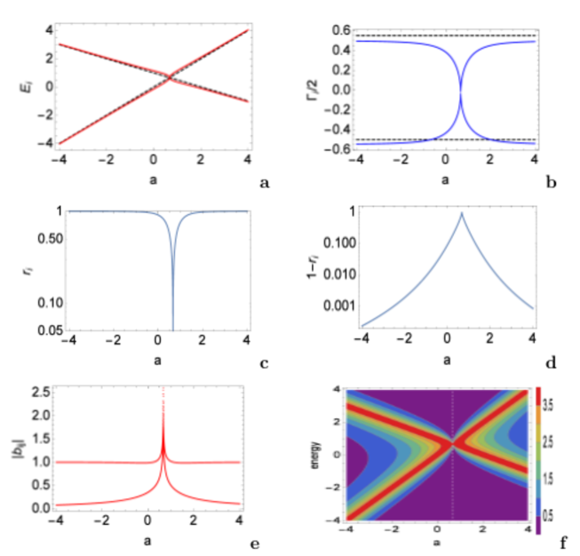
Figure 1: Eigenvalues ${\cal E}_{i}^{(1)}\equiv E_{i}^{(1)}+\frac{i}{2}\Gamma_{i}^{(1)}$ (a,b) and eigenfunctions $\Phi_{i}^{(1)}$ (c,d,e) of the Hamiltonian $\tilde{\cal H}^{(2,1)}$ as a function of $a$ and contour plot (f) of the cross section;  $\omega^{(1)}=0.5025$. Parameters: $e_{1}^{(1)}=1-a/2;~{}e_{2}^{(1)}=a;~{}\gamma_{1}^{(1)}/2=0.55;~{}\gamma_{2}^{(1)}/2=-0.5$ (dashed lines in a, b).

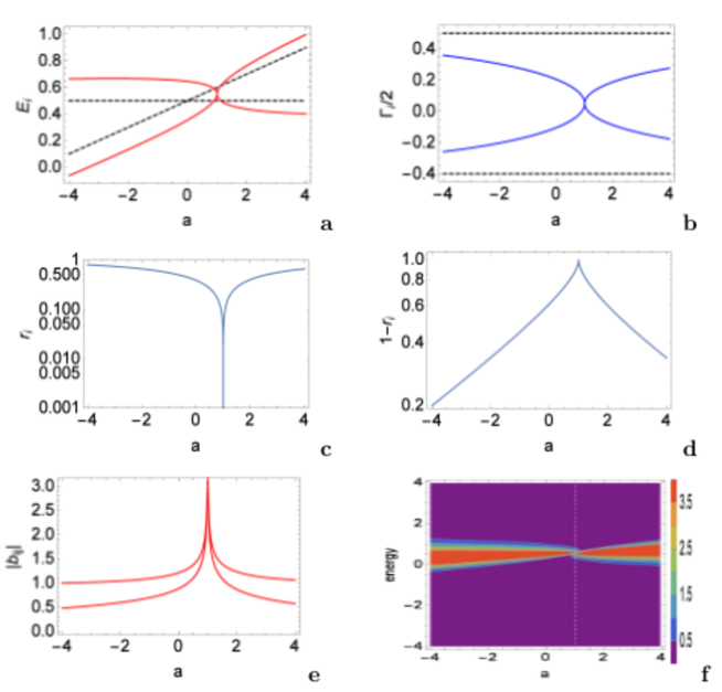
Figure 2: The same as Fig. 1 but $\omega^{(1)}=0.45+0.05i$ and $e_{1}^{(1)}=0.5;~{}e_{2}^{(1)}=0.5+0.1a;~{}\gamma_{1}^{(1)}/2=0.5;~{}\gamma_{2}^{(1)}/2=-0.4$.

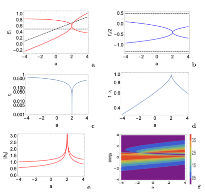
Figure 3: The same as Fig. 1 but $\omega^{(1)}=0.9+0.1i$ and $e_{1}^{(1)}=0.5;~{}e_{2}^{(1)}=0.5+0.1a;~{}\gamma_{1}^{(1)}/2=0.5;~{}\gamma_{2}^{(1)}/2=-1.3$.

II.6.1 Merge of states with gain and loss

Let us first consider the results that are obtained by using a parametric dependence of the energies $e_{i}^{(1)}$ and widths $\gamma_{i}^{(1)}$ of the states of the localized part of the system which is analog to that used in epj1 ; proj10 for a decaying system. The results are shown in Fig. 1.

In this figure, the existence of an EP at the parameter value $a=a^{\rm cr}=2/3$ can clearly be seen. Here, the two states are exchanged (Figs. 1.a,b), the phase rigidity $r_{i}$ approaches the value $0$ (Figs. 1.c, d) and the EM of the states via the continuum increases limitless (Fig. 1.e). The contour plot of the cross section (Fig. 1.f) shows the wavefunctions of the two states: while the eigenvalues of $\tilde{\cal H}^{(2,1)}$ cannot be seen according to (28) and (29), the eigenfunctions show some fluctuating behavior around the positions of the eigenstates according to the finite (nonvanishing) range of their influence (see Figs. 1.c,d,e). These fluctuations of the eigenfunctions can be seen in the contour plot. Although they follow the positions of the eigenvalues, their nature is completely different from that of the eigenvalue trajectories. The eigenfunction trajectories in Fig. 1.f show the exchange of the two states at the EP. That means: the state with positive width turns into a state with negative width and vice versa. This underlines once more that the two trajectories shown in Fig. 1.f have really nothing in common with the eigenvalue trajectories of resonance states the widths of which are always negative (or zero at most).

We underline once more that the results shown in Fig. 1 are formally similar to those obtained and discussed in epj1 ; proj10 for a decaying system. In the latter case, both states which are exchanged at the EP, are of the same type: they are resonance states with negative widths. It is interesting to see from the numerical results (Fig. 1), that the non-Hermitian Hamilton operator $\cal H$ can be used, indeed, for the description of these two different types of open quantum systems as suggested in Sect. II comment3 .

Additionally we show some numerical results for the case that, respectively, the distance in energy of the two states is smaller (Fig. 2) and the EM as well as the widths $|\gamma_{i}^{(1)}|$ differ more from one another (Fig. 3) than in Fig. 1. The eigenvalue and eigenfunction figures (Figs. 1.a-e,  2.a-e,  3.a-e) are similar to one another and show clearly the signatures of an EP at a certain critical value of the parameter $a=a_{\rm cr}$. The contour plots (Fig. 1.f,  2.f,  3.f) differ however from one another.

When the states are nearer to one another in energy, the two states with negative and positive width merge (Fig. 2.f). Under the influence of stronger EM (stronger coupling strength $\omega^{(1)}$ between system and environment) as well as of a larger difference between the two values $|\gamma_{i}^{(1)}|$, the extension of the region with non-vanishing cross section is enlarged in relation to the energy (Fig. 3.f). In any case, the cross section vanishes around $a=a_{\rm cr}$. Resonance states are not excited.

II.6.2 Level repulsion of states with gain and loss

More characteristic for an open quantum system with gain and loss than those in Sect. II.6.1 are the analytical results given in Sect. II.5. According to these results, the cross section is zero when $\gamma_{1}^{(1)}=-\gamma_{2}^{(1)}$,  $e_{1}^{(1)}=e_{2}^{(1)}$, and $\omega^{(1)}\in\Re$. Under the influence of an EP which causes differences between the original spectroscopic values $\varepsilon_{i}^{(1)}\equiv e_{i}^{(1)}+\frac{i}{2}\gamma_{i}^{(1)}$ and the eigenvalues ${\cal{E}}_{i}^{(1)}\equiv E_{i}^{(1)}+\frac{i}{2}\Gamma_{i}^{(1)}$ of $\tilde{\cal H}^{(2,1)}$, a non-vanishing cross section is expected when at least one of the conditions $\Gamma_{1}^{(1)}=-\Gamma_{2}^{(1)}$,  $E_{1}^{(1)}=E_{2}^{(1)}$, together with $\omega^{(1)}\in\Re$, is not fulfilled.

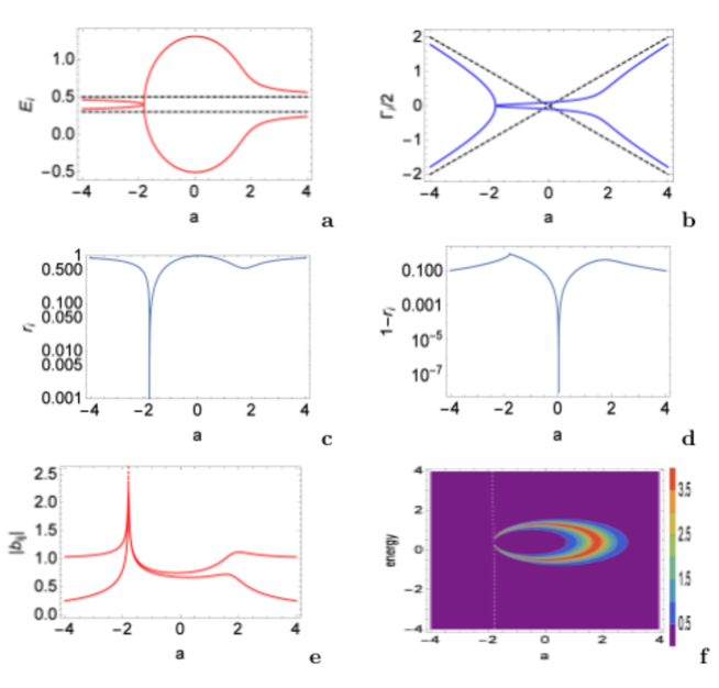
Figure 4: The same as Fig 1 but $\omega^{(1)}=0.9+0.1i$ and $e_{1}^{(1)}=0.5;~{}e_{2}^{(1)}=0.3;~{}\gamma_{1}^{(1)}/2=0.5a;~{}\gamma_{2}^{(1)}/2=-0.5a$.

In Fig. 4 we show the corresponding numerical results obtained for two neighboring states, $e_{1}^{(1)}\approx e_{2}^{(1)}$, and $\omega^{(1)}$ almost real. We fix the energies $e_{i}^{(1)}$ and vary parametrically the widths $\gamma_{i}^{(1)}$, see the dashed lines in Figs. 4.a,b. The results show an EP at $a=-1.8$ and the hint to another EP at $a=1.8$. At the EP, the phase rigidity approaches the value zero, $r_{i}\to 0$ (Fig. 4.c), and the EM of the states is extremely large, $|b_{ij}|\to\infty$ (Fig. 4.e).

Of special interest is the parameter range between the two EPs. Here, $r_{i}\to 1$ at $a\approx 0$ (Figs. 4.c,d). At this parameter value, the level repulsion is maximum; and the two eigenfunctions of the non-Hermitian Hamiltonian $\tilde{\cal H}^{(2,1)}$ are (almost) orthogonal.

An analogous result is known from calculations for decaying systems, i.e. for systems with excitation of resonance states top ; proj10 . In these calculations, the energies are varied parametrically and $\omega$ is almost imaginary (Fig. 1 in proj10 ). Therefore, the two eigenfunctions of the non-Hermitian Hamilton operator are (almost) orthogonal ($r_{i}\to 1$) at maximum width bifurcation (instead of at maximum level repulsion in Fig. 4).

In any case, the two eigenstates of the non-Hermitian operator turn irreversibly into two states with rigid phases in spite of the non-Hermiticity of the Hamiltonian. This unexpected result occurs due to the evolution of the system to the point of, respectively, maximum level repulsion and maximum width bifurcation, which is driven exclusively by the nonlinear source term of the Schrödinger equation, see Sect. II.4. The eigenfunctions of these two states are mixed.

In order to receive a better understanding of this result, we mention here another unexpected result of non-Hermitian quantum physics, namely the fact that a non-Hermitian Hamilton operator may have real eigenvalues comment3 . This fact is very well known in literature for a long time, for references see the review top . The corresponding states are called usually bound states in the continuum.

Most interesting for a physical system is the contour plot of the cross section (Fig. 4.f). According to the analytical results discussed in Sect. II.5, the cross section vanishes far from the parameter range that is influenced by an EP. It does however not vanish completely in the parameter range between the two EPs. Around the EP at $a=-1.8$, the conditions for vanishing cross section are quite well fulfilled, while this is not the case around the other EP at $a=1.8$. In approaching the two EPs by increasing and decreasing, respectively, the value of $a$ the cross section vanishes around $a=-1.8$, and is non-vanishing around $a=1.8$. The cross section vanishes also around the point of maximum level repulsion at which the two eigenfunctions of $\tilde{\cal H}^{(2,1)}$ are orthogonal (and not biorthogonal).

Additionally, we performed calculations (not shown in the paper) with the reduced value $\omega^{(1)}_{red}=0.5(0.9+0.1i)$ in order to determine the role of EM in the cross section picture. The obtained results are similar to those shown in Figs. 4.a-f. The parameter range influenced by the two EPs is however smaller when $\omega^{(1)}$ is reduced: it ranges from $a\approx-1$ to $a\approx 1$ when $\omega^{(1)}=\omega^{(1)}_{red}$. Accordingly, the region of the non-vanishing cross section in the contour plot shrinks in relation to $a$, and also in relation to the energy. In calculations with vanishing external mixing ($\omega^{(1)}=0$), the cross section vanishes everywhere.

III Open quantum system with gain and loss coupled to two environments

III.1 Hamiltonian for coupling to two environments

Let us consider the $4\times 4$ non-Hermitian matrix

$${\tilde{\cal H}^{(2,2)}}=\left(\begin{array}[]{cccc}\varepsilon_{1}^{(1)}&~{}~{}~{}~{}\omega^{(1)}&0&0\\ \omega^{(1)}&~{}~{}~{}~{}\varepsilon_{2}^{(1)}&0&0\\ 0&0&\varepsilon_{1}^{(2)}&~{}~{}~{}~{}\omega^{(2)}\\ 0&0&\omega^{(2)}&~{}~{}~{}~{}\varepsilon_{2}^{(2)}\\ \end{array}\right)\;.$$ (34)

Here, $\varepsilon_{i}^{(1)}\equiv e_{i}^{(1)}+\frac{i}{2}\gamma_{i}^{(1)}$ and $\varepsilon_{i}^{(2)}\equiv e_{i}^{(2)}+\frac{i}{2}\gamma_{i}^{(2)}$ are the complex eigenvalues of the basic non-Hermitian operator $\tilde{\cal H}^{(2,2)}$ relative to channel $c=1$ and $c=2$, respectively comment1 . The two channels (environments) are independent of and orthogonal to one another what is expressed by the zeros in the matrix (34). One of the channels may be related to gain and loss comment3 (acceptor and donor) considered in the previous section II, while the other channel may simulate a sink. In this case, the two widths $\gamma_{1}^{(1)}$ and $\gamma_{2}^{(1)}$ have different sign relative to the first channel. Relative to the second channel however, both $\gamma_{i}^{(2)}$ are negative according to a usual decay process of a resonance state.

The $\omega^{(1)}$ and $\omega^{(2)}$ stand for the coupling matrix elements between the two states $i=1,~{}2$ of the localized part of the open quantum system and the environment $c=1$ and $2$, respectively. In the case considered above, these two environments are completely different from one another and should never be related to one another. In more detail: an EM of the considered states may be caused only by $\omega^{(1)}$ or by $\omega^{(2)}$, and never by both values at the same time comment5 . This is guaranteed when $\omega^{(2)}=0$ what is fulfilled when there is only one state in the second channel. When there are more states, then $|\omega^{(2)}|$ should be much smaller than $|\omega^{(1)}|$ (here we point to the general result that the values $\omega$ are related to the widths $\gamma_{i}$ of the states top ).

The values $|\gamma_{i}^{(1)}|$ and $|\gamma_{i}^{(2)}|$ are independent of one another and express the different time scales characteristic of the two channels. While the $|\gamma_{i}^{(1)}|$ will be usually very large, the $|\gamma_{i}^{(2)}|$ are generally much smaller. Accordingly, the two-step process as a whole will show, altogether, a bi-exponential decay: first the decay occurs due to the exponential quick process; somewhere at its tail it will however switch over into the exponential decay of the slow process.

The Hamiltonian which describes vanishing coupling of the states of the localized part of the open quantum system to both environments is

$$\tilde{\cal H}_{0}^{(2,2)}=\left(\begin{array}[]{cccc}\varepsilon_{1}^{(1)}&0&0&0\\ 0&~{}~{}~{}~{}\varepsilon_{2}^{(1)}&0&0\\ 0&0&\varepsilon_{1}^{(2)}&0\\ 0&0&0&~{}~{}~{}~{}\varepsilon_{2}^{(2)}\\ \end{array}\right)$$ (39)

by analogy to (6). It does not contain any EM via an environment.

III.2 Eigenvalues and eigenfunctions of $\tilde{\cal H}^{(2,2)}$

The eigenvalues ${\cal E}_{i}^{(c)}\equiv E_{i}^{(c)}+\frac{i}{2}\Gamma_{i}^{(c)}$ and eigenfunctions $\Phi_{i}^{(c)}$ of (34) are characterized by two numbers: the number $i$ of the state ($i=1,2$) of the localized part of the system and the number $c$ of the channel ($c=1,2$), called environment, in which the system is embedded. Generally, $E_{i}^{(1)}\neq E_{i}^{(2)}$ and $\Gamma_{i}^{(1)}\neq\Gamma_{i}^{(2)}$. Also the wave functions $\Phi_{i}^{(1)}$ and $\Phi_{i}^{(2)}$ differ from one another due to the EM of the eigenstates via the environment $c=1$ and $c=2$, respectively. From a mathematical point of view, the system has therefore four states.

An EP influences the dynamics of the open quantum system also in the two-channel case. Without an EP in the considered parameter range in relation to both channels, we have $E_{i}^{(1)}\approx E_{i}^{(2)}$, $\Gamma_{i}^{(1)}\approx\Gamma_{i}^{(2)}$ and $\Phi_{i}^{(1)}\approx\Phi_{i}^{(2)}$. Accordingly, one has to consider effectively only two states

Under the influence of an EP relative to $c=1$ (or/and relative to $c=2$), the eigenvalues and eigenfunctions will be, however, different from one another, $E_{i}^{(1)}\neq E_{i}^{(2)}$, $\Gamma_{i}^{(1)}\neq\Gamma_{i}^{(2)}$ and $\Phi_{i}^{(1)}\neq\Phi_{i}^{(2)}$ in the corresponding parameter range. We have to consider therefore effectively four states in this case.

According to kato an EP is defined when the system is embedded in one common environment. Under this condition, it causes nonlinear processes in a physical system, which is the crucial factor for the dynamical properties of an open quantum system top . This is valid not only for systems all states of which decay (corresponding to some loss), but also for systems with loss and gain, as shown in top .

Due to the nonlinear processes occurring near to an EP, it is difficult to receive analytical solutions for the eigenvalues and eigenfunctions of (34). We will provide the results of some numerical simulations, above all with $e_{1}^{(1)}\approx e_{2}^{(1)}$, almost real $\omega^{(1)}$ and almost imaginary $\omega^{(2)}$, which is the most interesting and general case for a system with gain and loss that is coupled to a sink (see the analytical results obtained with $e_{1}^{(1)}=e_{2}^{(1)}$ and $\omega^{(1)}\in\Re$, Eq. (9), and the corresponding results for decaying systems in proj10 ).

III.3 Schrödinger equation with source term and coupling to two environments

Using (34), we can write down the Schrödinger equation with source term for the two-channel case in analogy to (25) for the one-channel case. The corresponding equation reads

$$({\cal H}^{(2,2)}_{0}-{\cal E}_{i}^{(c)})~{}|\Phi_{i}^{(c)}\rangle=-\left(\begin{array}[]{cccc}0&\omega^{(1)}&0&0\\ \omega^{(1)}&0&0&0\\ 0&0&0&\omega^{(2)}\\ 0&0&\omega^{(2)}&0\end{array}\right)|\Phi_{i}^{(c)}\rangle\;.$$ (44)

The source term depends on the coupling of the system to both channels, i.e. on $\omega^{(1)}$ and on $\omega^{(2)}$. We will consider the general case with two channels (two environments) in which $|\omega^{(2)}|\ll|\omega^{(1)}|$.

We repeat here that, according to their definition kato , EPs occur only in the one-channel case, i.e. only in the submatrices related either to channel $1$ or to channel $2$. They are not defined in the $4\times 4$ matrix (34). However, each EP in one of the two submatrices in (34) influences the dynamics of the open two-channel system. This will be shown in the following section by means of numerical results for the case that there is an EP in the first channel which simulates acceptor and donor (gain and loss), while the second channel being of standard type with resonance states, may or may not have an EP.

III.4 Numerical results: two-channel case

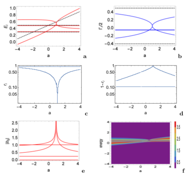
Figure 5: Eigenvalues ${\cal E}_{i}^{(1,2)}\equiv E_{i}^{(1,2)}+\frac{i}{2}\Gamma_{i}^{(1,2)}$ (a,b) and eigenfunctions $\Phi_{i}^{(1,2)}$ (c,d,e) of the Hamiltonian $\tilde{\cal H}^{(2,2)}$ and contour plot (f) of the cross section as function of $a$ with two merging states in the first channel, $\omega^{(2)}=0.005+0.045~{}i$. $~{}e_{1}^{(2)}=0.5;~{}e_{2}^{(2)}=0.3;~{}\gamma_{1}^{(2)}/2=-0.05;~{}\gamma_{2}^{(2)}/2=-0.05$ (dashed lines in a, b). The parameters of the first channel are the same as those in Fig. 2.

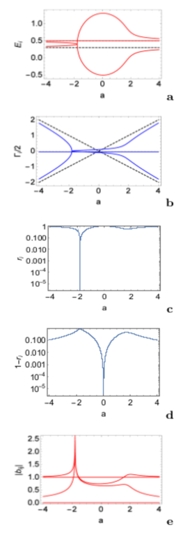
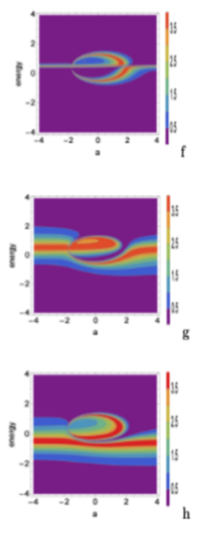
Figure 6: Left: Eigenvalues ${\cal E}_{i}^{(1,2)}\equiv E_{i}^{(1,2)}+\frac{i}{2}\Gamma_{i}^{(1,2)}$ (a,b) and eigenfunctions $\Phi_{i}^{(1,2)}$ (c,d,e) of the Hamiltonian $\tilde{\cal H}^{(2,2)}$ as function of $a$ with one state in the second channel, $\omega^{(2)}=0$. $~{}e_{1}^{(2)}=0.5;~{}\gamma_{1}^{(2)}/2=-0.05$ (dashed lines in a, b). The parameters of the first channel are the same as those in Fig. 4. Right: contour plots of the cross section with the same parameters of the first channel as in Fig. 4; $\omega^{(2)}=0$; and (f) $~{}e_{1}^{(2)}=0.5;~{}\gamma_{1}^{(2)}/2=-0.05$; (g) $~{}e_{1}^{(2)}=0.5;~{}\gamma_{1}^{(2)}/2=-0.5$; (h) $~{}e_{1}^{(2)}=-0.5;~{}\gamma_{1}^{(2)}/2=-0.5$.

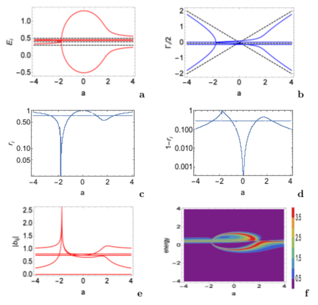
Figure 7: Eigenvalues ${\cal E}_{i}^{(1,2)}\equiv E_{i}^{(1,2)}+\frac{i}{2}\Gamma_{i}^{(1,2)}$ (a,b) and eigenfunctions $\Phi_{i}^{(1,2)}$ (c,d,e) of the Hamiltonian $\tilde{\cal H}^{(2,2)}$ and contour plot (f) of the cross section as function of $a$ with two states in the second channel, $\omega^{(2)}=0.01+0.09~{}i$. $~{}e_{1}^{(2)}=0.4;~{}e_{2}^{(2)}=0.5;~{}\gamma_{1}^{(2)}/2=-0.06;~{}\gamma_{2}^{(2)}/2=-0.06$ (dashed lines in a, b). The parameters of the first channel are the same as those in Fig. 4.

We performed some calculations for the two-channel case by starting from the calculations for the one-channel case in, respectively, Fig. 2 and 4 and by adding a second channel that describes decaying states (corresponding to loss). There are, of course, very many possibilities for choosing the number of states as well as the parameters for the second channel. One possibility is to keep the parameters constant by varying the parameter $a$ of the first channel. Another possibility is to relate them directly to the parameter $a$, or to introduce another independent parameter $b$. The choice should correspond to the physical situation considered.

The aim of our calculations is to illustrate the influence of a second channel onto the eigenvalues and eigenfunctions of $\tilde{\cal H}^{(2,2)}$ and onto the contour plot of the cross section. We exemplify this by choosing parameter dependent values $\varepsilon_{i}^{(1)}$ in the first channel and parameter independent values $\varepsilon_{i}^{(2)}$ in the second channel. In the following, we show a few characteristic results.

III.4.1 Merge of states with gain and loss; second channel with two states

We start these calculations with two channels by choosing two merged states with gain and loss according to Fig. 2. The second channel contains two resonance states $i=1,2$ with negative widths and $|\gamma_{i}^{(2)}|\ll|\gamma_{i}^{(1)}|$, see Fig. 5. The eigenvalue and eigenfunction pictures Fig. 5.a,b and c,d,e, respectively, show the eigenvalues and eigenfunctions of the first channel (Fig. 2.a-e) as well as the eigenvalues and eigenfunctions of the second channel. The last ones are constant as function of the parameter $a$ what follows from the assumption of their parameter independence.

The contour plots of the cross section (Figs. 2.f and 5.f) are different from one another. Common to both of them is that the cross section does not vanish in a finite range of the energy around $E\approx 0$ for all $a$. Under the influence of the two states in the second channel which are exactly in this energy and parameter range, the cross section is somewhat reduced. It does however not vanish.

These (and similar) simulations show clearly the following result. The fluctuations of the cross section which are caused by the merging of two states with gain and loss in the first channel, excite resonance states in the second channel. This happens although the nature of both channels is completely different. In the first channel, internal degrees of freedom of the system are not excited, while the appearance of the resonance states in the second channel occurs via excitation of internal degrees of freedom of the system.

III.4.2 Level repulsion of states with gain and loss; second channel with one state

In these calculations we start from the results shown in Fig. 4 for the first channel. The second channel contains only one state. The eigenvalue and eigenfunction pictures Fig. 6.a-e contain the eigenvalues and eigenfunction trajectories of Fig. 4.a-e as well as those of the second channel, e.g. the energy trajectories at $E_{i}=0.5$ and width trajectories at $\Gamma_{i}/2=-0.05$. The phase rigidity approaches the value $1$ at $a=0$ in both cases.

The corresponding contour plot of the cross section is shown in Fig. 6.f. It is related to the contour plot of the first channel (Fig. 4.f); and shows additionally the parameter independent state of the second channel in the whole parameter range.

We performed further calculations with parameters similar to those used in Fig. 6.a-e and show two of the corresponding contour plots in Figs. 6.g,h. Both contour plots are obtained with the comparably large width $\gamma_{1}^{(2)}/2=-0.5$; the two energies $e_{1}^{(2)}$ are however different from one another. The difference between $e_{1}^{(2)}=0.5$ and $e_{1}^{(2)}=-0.5$ can clearly seen in the corresponding contour plots Figs. 6.g and h.

The results of these simulations with level repulsion in the first channel and one state in the second channel show the same characteristic features as those discussed above for merging states. The fluctuations observed in the first channel are able to excite resonance states in the second channel.

III.4.3 Level repulsion of states with gain and loss; second channel with two states

The situation with two states in the second channel is richer than that with only one state because the two states can mix via the common continuum. We show results for one special case in Fig. 7. As in Figs. 5 and 6, the eigenvalue figures 7.a,b contain the eigenvalue trajectories of both channels. The eigenfunction trajectories refer to the existence of an EP in the second channel: the phase rigidity of states related to the second channel is independent of the parameter $a$, as expected. It is however smaller than $1$. Also the mixing $|b_{ij}|$ of the two wavefunctions via the common continuum in the second channel shows small deviations from the expectations. The relation of these results for the eigenfunctions of ${\cal H}^{(2,2)}$ to an EP in the second channel is discussed in detail in appendix A.

The contour plot Fig. 7.f shows the same characteristic features as Fig. 6.f. Both, its relation to the contour plot of the first channel (Fig. 4.f) as well to the parameter independent state of the second channel can clearly be seen. Thus, the fluctuations observed in the first channel excite resonance states in the second channel also in this case.

Summarizing the numerical results shown in the three figures 5 to 7 we state the following. Gain and loss in the first channel and excitation of resonance states in the second channel are a uniform process. This process can be described as a whole in the formalism for the description of open quantum systems which is used in the present paper.

IV Discussion and summary of the results

In our paper, we considered gain and loss in an open quantum system comment3 . Of special interest is the interplay of these two opposed processes in the neighborhood of singular points where it causes fluctuations of the cross section. These fluctuations are observable and can excite resonance states in the system. The time scale of the fluctuations and that of the excitation of resonance states are very different. The fluctuations of the cross section occur quickly, without any excitation of internal degrees of freedom of the system. The excitation of resonance states is however much slower, and internal degrees of freedom of the system are involved.

The results of our calculations meet therefore the condition that the lifetime of the primary process in the photosynthetic reaction center has to be very short. Otherwise the energy received from the photosynthetic excitation, will change into heat and fluorescence lakhno . This is a statement of Hermitian quantum physics, since the change of energy into heat and fluorescence is impossible in non-Hermitian quantum physics according to the results of our calculations. Here the photosynthesis does not excite any eigenstate of the non-Hermitian Hamiltonian $\cal H$. Instead, the primay process occurs due to fluctuations of the eigenfunctions of $\cal H$ around EPs. The mechanism of photosynthetic excitation in non-Hermitian quantum physics is therefore, as a matter of principle, different from that in Hermitian quantum physics.

We sketched first the formalism by means of which both the interplay between gain and loss in an open quantum system comment3 and the excitation of resonance states can be described as a uniform process. In any case, the widths $\gamma_{i}$ of the states are (generally) different from zero. In the first case we have two states with different sign of the widths (corresponding to gain and loss), while the states in the second case are standard decaying (resonance) states with negative sign comment1 .

Generally, the cross section related to the two states with gain and loss vanishes. Deviations from this rule appear around the position of an eigenstate and in the neighborhood of singular (exceptional) points, where they may cause non-vanishing fluctuations of the cross section. These fluctuations have nothing in common with resonances. Rather, they are merely deviations from the vanishing value of the cross section and are not related to the excitation of any internal degrees of freedom of the system. They occur therefore with an efficency of nearly 100 % at a very short time scale.

The fluctuations caused by the interplay of the states with gain and loss, are observable and may excite resonance states of the system after a comparably long time (which corresponds to the widths $\Gamma_{i}$ of these states). The whole process of gain and loss together with the excitation of resonance states is therefore characterized by two very different time scales: the quick process which creates the fluctuations, and the slow process which is related to the excitation of resonance states. The decay occurs thus bi-exponential. Initially, it is determined by the quick process of the interplay between gain and loss. Somewhere at its tail however, it will switch over to the slow process with excitation of internal degrees of freedom of the system.

The states with gain and loss as well as the resonance states excited by the fluctuations, can each interact via a common environment into which the corresponding states are embedded. The two environments (channels) will never mix. This request is guaranteed in our formalism due to the very different time scales of the two processes. In any case, this so-called external mixing of the states occurs additionally to the direct so-called internal mixing of the states which is supposed in our calculations to be involved in the complex energies $\varepsilon_{i}\equiv e_{i}+i\gamma_{i}/2$ of the states.

According to the numerical results of our paper, the fluctuations are very robust. They appear in a relatively large finite parameter range around the positions of the eigenstates and around EPs.

Finally, we mention a few interesting results which are characteristic of open quantum systems including those considered in the present paper.

1. The states of an open quantum system may interact via a common environment into which the system is embedded. This mixing is called usually external interaction.

2. The states of an open quantum system may have positive or negative widths. The states with positive width comment1 gain excitons (or information) from the environment while those with negative width lose excitons (or information) due to their coupling to the environment. As function of a parameter, gain may pass into loss and vice versa top .

3. The phases of the eigenfunctions of a non-Hermitian operator are, generally, not rigid, see Figs. 1 to 7 and top ; proj10 .

4. Irreversible processes determine the evolution of an open quantum system up to the occurrence of orthogonal eigenstates at maximum width or level repulsion, see Figs. 4, 6, 7 and top ; proj10 .

We mention further that results similar to those discussed above for systems with two states, appear also in calculations for systems with more than two states, see proj10 ; pra93 ; epj2 . This holds true also for systems with gain and loss.

V Conclusions

In our paper, we provided some results for a two-step process which we obtained in the framework of the non-Hermitian formalism top ; proj10 for the description of open quantum systems. The first step is the interplay between gain and loss of information (excitons) from an environment, while the second step is the excitation of a resonance state. The two steps are treated as two parts of the whole process.

The total process might simulate photosynthesis: the first step is the capture of light in the light-harvesting complex while the second step is the transfer of the excitation energy to the reaction center which stores the energy from the photon in chemical bonds. That means: gain simulates the acceptor for light, and loss stands for the donor which excites a resonance state and simulates the coupling to the sink. Altogether, the energy of the light is transferred to the reaction center of the light-harvesting complex. The obtained results are very robust, and fluctuations play an important role.

The results show some characteristic features which correspond, indeed, to those discussed in the literature for the photosynthesis. Most interesting are the following results of our calculations:

1. the efficency of energy transfer is nearly 100 %;

2. the energy transfer takes place at a very short time scale;

3. the storage of the energy in the reaction center occurs at a much longer time scale;

4. according to points 2 and 3, the decay is bi-exponential.

In future studies, the theoretical results have to be confirmed by application of the formalism to the description of concrete systems in close cooperation between theory and experiment.

Acknowledgment

We are indebted to J.P. Bird for valuable discussions.

Appendix A Exceptional point in the second channel

At an EP the two eigenfunctions of a non-Hermitian Hamilton operator $\cal H$ are exchanged according to (22). In more detail: tracing the eigenfunctions of $\cal H$ as function of a certain parameter $b$, the two eigenfunctions jump according to (22) at the critical parameter value $b=b^{\rm cr}$ which defines the position of the EP. Some years ago, it has been shown ro01 ; ro03 that the influence of the EP is not restricted to the jump occurring at $b^{\rm cr}$. It appears rather in a finite parameter range of $b$ in which the wavefunctions of the two states are mixed according to

$$\Phi_{i}^{\rm ch}=\beta_{k}\Phi_{k}\pm i\beta_{l}\Phi_{l}$$ (45)

with $k\neq l$. The two wavefunctions $\Phi_{i}^{\rm ch}$ vary smoothly (i.e. without any jump of the sign of their components) everywhere but at $b=b^{\rm cr}$. Using the representation

$$\Phi_{i}^{\rm ch}=|\Phi_{i}^{\rm ch}|e^{i\theta_{i}}$$ (46)

$\theta_{i}$ depends on the parameter $b$. After removing a common phase factor, it follows $\theta_{i}^{(1)}\to\pi/4$ and $\pm 3\pi/4$, respectively, in approaching $b=b^{\rm cr}$; and $\theta_{i}^{(2)}\to 0$ or $\pi$ when $b$ is far from the critical region around $b^{\rm cr}$. In between the values $\theta_{i}^{(1)}$ and $\theta_{i}^{(2)}$, the angle $\theta_{i}$ varies smoothly.

Corresponding to the dependence of $\theta_{i}$ on the parameter $b$, also the phase rigidity (20) depends on this parameter in a certain finite parameter range. The phase rigidity is determined by the ratio

$$r_{i}\equiv\frac{{\rm Re}(\beta_{k}+\beta_{l})^{2}}{|\beta_{k}+\beta_{l}|^{2}}$$ (47)

which approaches $0$ at the EP (due to $|\beta_{k}+\beta_{l}|^{2}\to\infty$) and $1$ far from the EP (because here the wavefunctions are almost real). The intermediate values of the phase rigidity $r_{i}$ are determined by the expression (47) calculated with the actual values $\beta_{k}$ and $\beta_{l}$. The results of these calculation give values for $r_{i}$ that are between the two limiting values $0$ and $1$.

Fig. 7 shows numerical results for the eigenfunctions of $\cal H$ which are obtained for calculations with two channels and two states in the second channel. We see the values $r_{i}$ for the states of the first channel (see Figs. 2 and 4) as well as those for the two states of the second channel. They are independent of one another. The $r_{i}$ related to the second channel are constant in the whole parameter range $a$ shown in the figures (which is defined for the first channel). They may be smaller than 1, see Fig. 7.

The results obtained for the phase rigidity $r_{i}$ of the two states in the second channel, may be considered as a proof of the finite parameter range in which an EP influences the properties of the system. The value $r_{i}$ is nothing but an expression for the distance of the system from an EP in the second channel: the larger $r_{i}$, the more distant is the EP, while $r_{i}\to 0$ indicates that the EP is approached. Thus, the value $r_{i}$ in the eigenfunction pictures of the two-channel system with two states in the second channel additionally to those of the one channel system (Figs. 2 and 4), allows us to determine the position of the EP in the second channel.

References

- (1) G. S. Engel, T. R. Calhoun, E. L. Read, T.-K. Ahn, T. Mancal, Y.-C. Cheng, R. E. Blankenship, and G. R. Fleming, Nature 446, 782 (2007)
-
(2)
H. Lee, Y.-C. Cheng, and G. R. Fleming, Science 316, 1462 (2007)
R.J. Sension, Nature 446, 740 (2007) - (3) M. Mohseni, Y. Omar, G.S. Engel, and M.B. Plenio (eds.), Quantum Effects in Biology, Cambridge University Press, Cambridge, UK, 2014
- (4) H. Dong and G. R. Fleming, J. Phys. Chem. B 118, 8956 (2014)
-
(5)
E. Romero, R. Augulis, V.I. Novoderezhkin, M. Ferretti, J. Thieme, D. Zigmantas, and R. van Grondelle, Nature Physics 10, 676 (2014)
S.F. Huelga and M.B. Plenio, Nature Physics 10, 621 (2014) - (6) J. S. Briggs and A. Eisfeld, Phys. Rev. E 83, 051911 (2011)
- (7) F. Caruso, A.W. Chin, A. Datta, S.F. Huelga, and M.B. Plenio, J. Phys. Chem. C 131, 105106 (2009)
-
(8)
M.O. Scully,
Phys. Rev. Lett. 104, 207701 (2010)
E. A. Sete, A. Svidzinsky, H. Eleuch, R. D. Nevels and M. O. Scully Journ. Mod. Opt. 57, 1311 (2010)
A.A. Svidzinsky, K.E. Dorfman, and M.O. Scully, Phys. Rev. A 84, 053818 (2011) - (9) V.D. Lakhno, Journ. Biological Physics 31, 145 (2005)
- (10) I. Rotter, J. Phys. A 42, 153001 (2009)
- (11) I. Rotter and J.P. Bird, Rep. Prog. Phys. 78, 114001 (2015)
- (12) P. Kleinwächter and I. Rotter, Phys. Rev. C 32, 1742 (1985)
- (13) N. Auerbach and V. Zelevinsky, Rep. Prog. Phys. 74, 106301 (2011)
- (14) G.L. Celardo, F. Borgonovi, M. Merkli, V.I. Tsifrinovich, and G.P. Berman, J. Phys. Chem. C 116, 22105 (2012)
-
(15)
D. Ferrari, G.L. Celardo, G.P. Berman, R.T. Sayre, and F. Borgonovi,
J. Phys. Chem. C 118, 20 (2014)
G.L. Celardo, G.G. Giusteri, and F. Borgonovi, Phys. Rev. B 90, 075113 (2014)
G.G.Giusteri, G.L. Celardo and F. Borgonovi, Phys. Rev. E 93, 032136 (2016) - (16) G.P. Berman, A.I. Nesterov, G.V. Lopez, and R.T. Sayre, J. Phys. Chem. C 119, 22289 (2015)
- (17) H. Eleuch and I. Rotter, Phys. Rev. A 95, 022117 (2017)
- (18) T. Kato, Perturbation Theory for Linear Operators, Springer, Berlin 1966
-
(19)
A.I. Nesterov, G.P. Berman, and A.R. Bishop,
Fortschr. Phys. 61, 95 (2013)
A.I. Nesterov, G.P. Berman, J.M.S. Martinez and R.T. Sayre, J. Math. Chem. 51, 2514 (2013) -
(20)
A.I. Nesterov and G.P. Berman,
Phys. Rev. E 91, 042702 (2015)
A.I. Nesterov and G.P. Berman, Phys. Rev. E 91, 052702 (2015) - (21) We underline that we consider open quantum systems with gain and loss. This should not be confused with the consideration of exactly balanced gain and loss in PT-symmetric systems which are neither open nor closed, but nonisolated according to the definition in, e.g., C.M. Bender, Journal of Physics: Conference Series 631, 012002 (2015).
- (22) In contrast to the definition that is used in, for example, nuclear physics, we define the complex energies before and after diagonalization of by and , respectively, with and for decaying states. This definition is useful when discussing systems with gain (positive widths) and loss (negative widths).
- (23) The coalescence of two eigenvalues of a non-Hermitian operator should not be confused with the degeneration of two eigenstates of a Hermitian operator. The eigenfunctions of two degenerate states are different and orthogonal while those of two coalescing states are biorthogonal and differ only by a phase, see Eq. (22).
- (24) I. Rotter, Phys. Rev. E 64, 036213 (2001)
- (25) A.I. Magunov, I. Rotter and S.I. Strakhova, J. Phys. B 34, 29 (2001)
- (26) U. Günther, I. Rotter and B.F. Samsonov, J. Phys. A 40, 8815 (2007)
- (27) B. Wahlstrand, I.I. Yakimenko, and K.F. Berggren, Phys. Rev. E 89, 062910 (2014)
- (28) F. Tellander and K.F. Berggren, Phys. Rev. A 95, 042115 (2017)
- (29) J.B. Gros, U. Kuhl, O. Legrand, F. Mortessagne, E. Richalot, and D. Savin, Phys. Rev. Lett. 113, 224101 (2014)
- (30) I. Rotter, Phys. Rev. E 68, 016211 (2003)
- (31) H. Eleuch and I. Rotter, Eur. Phys. J. D 69, 229 (2015)
- (32) Numerical calculations with have shown that, in such a case, the states of the second channel mix also via the first channel. The obtained results are abstruse from the point of view of physics, although they are mathematically correct.
- (33) H. Eleuch and I. Rotter, Phys. Rev. A 93, 042116 (2016)
- (34) H. Eleuch and I. Rotter, Eur. Phys. J. D 69, 230 (2015)