Open charm-bottom axial-vector tetraquarks and their properties

Abstract

The charged axial-vector $J^{P}=1^{+}$ tetraquarks $Z_{q}=[cq][\bar{b}\bar{q}]$ and $Z_{s}=[cs][\bar{b}\bar{s}]$ with the open charm-bottom contents are studied in the diquark-antidiquark model. The masses and meson-current couplings of these states are calculated by employing QCD two-point sum rule approach, where the quark, gluon and mixed condensates up to eight dimensions are taken into account. These parameters of the tetraquark states $Z_{q}$ and $Z_{s}$ are used to analyze the vertices $Z_{q}B_{c}\rho$ and $Z_{s}B_{c}\phi$ to determine the strong $g_{Z_{q}B_{c}\rho}$ and $g_{Z_{s}B_{c}\phi}$ couplings. For these purposes, QCD light-cone sum rule method and its soft-meson approximation are utilized. The couplings $g_{Z_{q}B_{c}\rho}$ and $g_{Z_{s}B_{c}\phi}$, extracted from this analysis, are applied for evaluating of the strong $Z_{q}\to B_{c}\rho$ and $Z_{s}\to B_{c}\phi$ decays’ widths, which are essential results of the present investigation. Our predictions for the masses of the $Z_{q}$ and $Z_{s}$ states are confronted with similar results available in the literature.

I Introduction

Charmonium-like states discovered during last years mainly in the exclusive B-meson decays as resonances in the relevant mass distributions became interesting objects for both experimental and theoretical studies in high energy physics. Conventional hadrons, composed of two and three quarks, and investigated in a rather detailed form constitute main part of the known particles. At the same time, the theory of the strong interactions – the Quantum Chromodynamics does not contain principles excluding an existence of the multiquark states. The tetraquark and pentaquark states composed of the four and five valence quarks, respectively, and hybrids built of the quarks and gluons are among most promising candidates to occupy the vacant shelves in the multiquark spectroscopy. Due to joint efforts of experimentalists and theorists considerable progress in understanding of the quark-gluon structure of the multiquark –exotic states and explaining of their properties were achieved, but remaining questions are more numerous that answered ones (for latest reviews, see Refs. Chen:2016qju ; Chen:2016spr ; Esposito:2014rxa ; Meyer:2015eta ).

The main source of problems, which complicates the studying of the charmonium-like tetraquarks, is the existence of the conventional charmonium states in the energy ranges of the exploring decay processes. Charmonia generate difficulties in interpretation of experimental results, because the pure $c\bar{c}$ states may emerge as the resonances in the mass distributions of the processes, or generate background effects due to states dynamically connected with $c\bar{c}$ levels. Only after eliminating effects of the charmonium states in forming of the experimental data, observed resonances can be considered as real exotic particles. The well-known $X(3872)$ state is the best sample to illustrate existing problems. It was discovered as very narrow resonance in B meson decay $B\to KX\to KJ/\psi\rho\to KJ/\psi\pi^{+}\pi^{-}$ by the Belle Collaboration Belle:2003 , and was later confirmed in CDF, D0 and BaBar experiments (see, Refs. CDF:2004 ; D0:2004 ; BaBar:2005 ). Its other production mechanisms running through decay chains $B\to KX\to KJ/\psi\omega\to KJ/\psi\pi^{+}\pi^{-}\pi^{0}$, $B\to KX\to KJ/\psi\gamma$ and $B\to KX\to K\psi(2S)\gamma$ were also experimentally measured and comprehensively studied Abe:2005ix ; Aubert:2008ae . The gathered information poses severe restrictions on theoretical models claiming to describe a behavior of the $X(3872)$ state. Attempts were made to explain the collected data by treating $X(3872)$ as the excited conventional charmonium $\chi_{c1}(2^{3}P_{1})$ Barnes:2005pb , or as the state formed due to dynamical coupled-channel effects Danilkin:2010cc . It was considered in the context of four-quark compounds, both as the $D\bar{D}^{\star}$ molecule or its admixtures with the charmonium states Close:2003sg ; Tornqvist:2004qy ; Zanetti:2011ju ; Guo:2014taa , and as the diquark-antidiquarks states Maiani:2004vq ; Maiani:2007vr ; Navarra:2006nd ; Dubnicka:2010kz ; Wang:2013vex .

But existence of the tetraquarks, which do not contain $\bar{c}c$ or $\bar{b}b$ pairs is also possible, because fundamental laws of QCD do not forbid production of such resonances in hadronic processes. These particles may appear in the exclusive reactions as the open charm (i.e., as states containing $c$ or $\bar{c}$ quarks) and open bottom resonances. The $D_{s0}^{\star}(2317)$ and $D_{s1}(2460)$ mesons discovered by the BaBar and CLEO collaborations Aubert:2003fg ; Besson:2003cp , are now being considered as candidates to open charm tetraquark states. The $X(5568)$ resonance remains a unique candidate to the open bottom tetraquark, which is also a particle containing four different quarks. Unfortunately, the experimental situation formed around $X(5568)$ remains unclear. Indeed, the evidence for $X(5568)$ was first announced by the D0 Collaboration in Ref. D0:2016mwd . Later it was seen again by D0 in the $B_{s}^{0}$ meson’s semileptonic decays D0 . Nevertheless, the LHCb and CMS collaborations could not see the same resonance from analysis of their experimental data Aaij:2016iev ; CMS:2016 . Theoretical investigations aiming to explain the nature of $X(5568)$ and calculate its parameters lead also to contradictory conclusions. Predictions obtained in some of these works are in a nice agreement with results of the D0 Collaboration, while in others even an existence of the $X(5568)$ state is an object of doubts. The detailed discussions of these and related questions of the $X(5568)$ state’ physics can be found in original works (see, Ref. Chen:2016spr and references therein).

The open charm-bottom tetraquarks belong to another type of exotic states. They already attracted an interest of physicists even till now were not observed experimentally. The original investigations of these particles started more than two decades ago, and, therefore, a considerable theoretical information on their expecting properties is available in the literature. For example, the open charm-bottom type tetraquarks with the contents $\{Qq\}\{Q^{\prime}q\}$, $\{Qs\}\{Q^{\prime}s\}$ and molecule structures were considered in Refs. Zhang:2009vs and Zhang:2009em , respectively. In these papers the masses of these hypothetical states were calculated in the context of QCD two-point sum rule approach using in the operator product expansion (OPE) the operators up to dimension six. In the framework of the diquark-antidiquark model the open charm-bottom states were analyzed in Ref. Chen:2013aba . In order to extract masses of these states, the authors again utilized QCD sum rule method and interpolating currents of different color structure. Other aspects of these tetraquark systems can be found in Refs. Zouzou:1986qh ; SilvestreBrac:1993ry ; Ebert:2007rn ; Sun:2012sy ; Albuquerque:2012rq .

In a previous article Agaev:2016dsg we explored the charged scalar $J^{P}=0^{+}$ tetraquark states $Z_{q}=[cq][\bar{b}\bar{q}]$ and $Z_{s}=[cs][\bar{b}\bar{s}]$ in the context of the diquark-antidiquark model, and calculated their masses and widths some of their decay channels. In the present work we extend our investigations by including into analysis the axial-vector $J^{P}=1^{+}$ $Z_{q}=[cq][\bar{b}\bar{q}]$ and $Z_{s}=[cs][\bar{b}\bar{s}]$ open charm-bottom tetraquarks, and their kinematically allowed decay modes.

We start from calculation of their masses and meson-current couplings. For these purposes, we employ QCD two-point sum rule method, which was invented to calculate parameters of the conventional hadrons Shifman:1979 , but soon was applied to analysis of the exotic states, as well (see, Refs. Braun:1985ah ; Braun:1988kv ; Balitsky:1982ps ; Reinders:1985 ). The parameters of the open charm-bottom tetraquarks obtained within this method are used to explore the strong vertices $Z_{q}B_{c}\rho$ and $Z_{s}B_{c}\phi$, and calculate the corresponding couplings $g_{Z_{q}B_{c}\rho}$ and $g_{Z_{s}B_{c}\phi}$. These couplings are required to evaluate the widths of the $Z_{q}\rightarrow B_{c}\rho$ and $Z_{s}\rightarrow B_{c}\phi$ decays. To this end, we apply QCD light-cone sum method and soft-meson approximation proposed in Refs. Braun:1989 ; Ioffe:1983ju ; Braun:1995 . For analysis of the strong vertices of tetraquarks the method was, for the first time, examined in Ref. Agaev:2016dev , and afterwards successfully used to investigate decay channels of some tetraquarks states (see, Refs. Agaev:2016ijz ; Agaev:2016lkl ; Agaev:2016urs ).

The present work is organized in the following manner. In Sec. II we calculate the masses and meson-current couplings of the axial-vector tetraquarks with open charm-bottom contents. Section III is devoted to computation of the strong couplings $g_{Z_{q}B_{c}\rho}$ and $g_{Z_{s}B_{c}\phi}$. In this section we calculate the widths of the decays $Z_{q}\rightarrow B_{c}\rho$ and $Z_{s}\rightarrow B_{c}\phi$. In Sec. IV we examine our results as a part of the general tetraquark’s physics and compare them with predictions of Ref. Chen:2013aba , where the masses of the axial-vector open charm-bottom tetraquarks were found. It contains also our concluding remarks.

II Masses and meson-current couplings

In order to find the masses and meson-current couplings of the diquark-antidiquark type axial-vector states $Z_{q}$ and $Z_{s}$, we use the two-point QCD sum rules. Below the explicit expressions for the $Z_{q}$ state are written down. Their generalization to embrace $Z_{s}$  tetraquark is straightforward.

The two-point sum rule can be extracted from analysis of the correlation function

$$\Pi_{\mu\nu}(p)=i\int d^{4}xe^{ipx}\langle 0|\mathcal{T}\{J_{\mu}(x)J_{\nu}^{{\dagger}}(0)\}|0\rangle,$$ (1)

where $J_{\mu}$ is the interpolating current of the $Z_{q}$ state.

The scalar and axial-vector open charm-bottom diquark-antidiquark states can be modeled using different type of interpolating currents Chen:2013aba . Thus, the interpolating currents can be either symmetric or antisymmetric in the color indices. In our previous work we chose the symmetric interpolating current to find masses and decay widths of the scalar open charm-bottom tetraquarks Agaev:2016dsg . In the present work to consider the axial-vector tetraquark states $Z_{q}$ and $Z_{s}$ we use again the interpolating currents, which are symmetric in the color indices. Such axial-vector current has the following form

$$J_{\mu}=q_{a}^{T}C\gamma_{5}c_{b}\left(\overline{q}_{a}\gamma_{\mu}C\overline{b}_{b}^{T}+\overline{q}_{b}\gamma_{\mu}C\overline{b}_{a}^{T}\right),$$ (2)

and is symmetric under exchange of the color indices $a\leftrightarrow b$. Here by $C$ we denote the charge conjugation matrix.

To derive QCD sum rules for the mass and meson-current coupling we follow standard prescriptions of the sum rule method and express the correlation function $\Pi_{\mu\nu}(p)$ in terms of the physical parameters of the $Z_{q}$ state, which results in obtaining $\Pi_{\mu\nu}^{\mathrm{Phys}}(p)$. From another side the same function should be obtained in terms of the quark-gluon degrees of freedom $\Pi_{\mu\nu}^{\mathrm{QCD}}(p)$.

We start from the function $\Pi_{\mu\nu}^{\mathrm{Phys}}(p)$ and compute it by suggesting, that the tetraquarks under consideration are the ground states in the relevant hadronic channels. After saturating the correlation function with a complete set of the $Z_{q}$ states and performing in Eq. (1) integration over $x$ , we get the required expression for $\Pi_{\mu\nu}^{\mathrm{Phys}}(p)$

$$\Pi_{\mu\nu}^{\mathrm{Phys}}(p)=\frac{\langle 0|J_{\mu}|Z_{q}(p)\rangle\langle Z_{q}(p)|J_{\nu}^{{\dagger}}|0\rangle}{m_{Z}^{2}-p^{2}}+...$$

where $m_{Z}$ is the mass of the $Z_{q}$ state, and dots indicate contributions coming from higher resonances and continuum states. We introduce the meson-current coupling $f_{Z}$ by means of the equality

$$\langle 0|J_{\mu}|Z_{q}(p)\rangle=f_{Z}m_{Z}\varepsilon_{\mu},$$

where $\varepsilon_{\mu}$ is polarization vector of the axial-vector tetraquark. In terms of $m_{Z}$ and $f_{Z}$ the correlation function takes the simple form

$$\Pi_{\mu\nu}^{\mathrm{Phys}}(p)=\frac{m_{Z}^{2}f_{Z}^{2}}{m_{Z}^{2}-p^{2}}\left(-g_{\mu\nu}+\frac{p_{\mu}p_{\nu}}{m_{Z}^{2}}\right)+\ldots$$ (3)

Having applied the Borel transformation to the function $\Pi_{\mu\nu}^{\mathrm{Phys}}(p)$ we get

$$\mathcal{B}_{p^{2}}\Pi_{\mu\nu}^{\mathrm{Phys}}(p^{2})=m_{Z}^{2}f_{Z}^{2}e^{-m_{Z}^{2}/M^{2}}\left(-g_{\mu\nu}+\frac{p_{\mu}p_{\nu}}{m_{Z}^{2}}\right)+\ldots$$ (4)

In order to obtain the function $\Pi_{\mu\nu}^{\mathrm{QCD}}(p)$ we substitute the interpolating current given by Eq. (2) into Eq. (1), and employ the light and heavy quark propagators in calculations. For $\Pi_{\mu\nu}^{\mathrm{QCD}}(p)$, as a result, we get:

$$\Pi_{\mu\nu}^{\mathrm{QCD}}(p)=i\int d^{4}xe^{ipx}\left\{\mathrm{Tr}\left[\gamma_{\mu}\widetilde{S}_{b}^{b^{\prime}b}(-x)\gamma_{\nu}S_{q}^{a^{\prime}a}(-x)\right]\right.$$

$$\times\mathrm{Tr}\left[\gamma_{5}\widetilde{S}_{q}^{aa^{\prime}}(x)\gamma_{5}S_{c}^{bb^{\prime}}(x)\right]+\mathrm{Tr}\left[\gamma_{\mu}\widetilde{S}_{b}^{a^{\prime}b}(-x)\right.$$

$$\times\left.\gamma_{\nu}S_{q}^{b^{\prime}a}(-x)\right]\mathrm{Tr}\left[\gamma_{5}\widetilde{S}_{q}^{aa^{\prime}}(x)\gamma_{5}S_{c}^{bb^{\prime}}(x)\right]$$

$$+\mathrm{Tr}\left[\gamma_{\mu}\widetilde{S}_{b}^{b^{\prime}a}(-x)\gamma_{\nu}S_{q}^{a^{\prime}b}(-x)\right]\mathrm{Tr}\left[\gamma_{5}\widetilde{S}_{q}^{aa^{\prime}}(x)\gamma_{5}S_{c}^{bb^{\prime}}(x)\right]$$

$$\left.+\mathrm{Tr}\left[\gamma_{\mu}\widetilde{S}_{b}^{a^{\prime}a}(-x)\gamma_{\nu}S_{q}^{b^{\prime}b}(-x)\right]\mathrm{Tr}\left[\gamma_{5}\widetilde{S}_{q}^{aa^{\prime}}(x)\gamma_{5}S_{c}^{bb^{\prime}}(x)\right]\right\},$$

where

$$\widetilde{S}_{q(b)}^{ab}(x)=CS_{q(b)}^{Tab}(x)C,$$ (6)

with $S_{q}(x)$ and $\ S_{b}(x)$ being the $q$- and $b$-quark propagators, respectively.

We proceed including into analysis the well known expressions of the light and heavy quark propagators. For our aims it is convenient to use the $x$-space expression of the light quark propagator,

$$S_{q}^{ab}(x)=i\delta_{ab}\frac{\not{x}}{2\pi^{2}x^{4}}-\delta_{ab}\frac{m_{q}}{4\pi^{2}x^{2}}-\delta_{ab}\frac{\langle\overline{q}q\rangle}{12}$$

$$+i\delta_{ab}\frac{\not{x}m_{q}\langle\overline{q}q\rangle}{48}-\delta_{ab}\frac{x^{2}}{192}\langle\overline{q}g_{s}\sigma Gq\rangle+i\delta_{ab}\frac{x^{2}\not{x}m_{q}}{1152}\langle\overline{q}g_{s}\sigma Gq\rangle$$

$$-i\frac{g_{s}G_{ab}^{\alpha\beta}}{32\pi^{2}x^{2}}\left[\not{x}{\sigma_{\alpha\beta}+\sigma_{\alpha\beta}}\not{x}\right]-i\delta_{ab}\frac{x^{2}\not{x}g_{s}^{2}\langle\overline{q}q\rangle^{2}}{7776}$$

$$-\delta_{ab}\frac{x^{4}\langle\overline{q}q\rangle\langle g_{s}q^{2}G^{2}\rangle}{27648}+\ldots.$$ (7)

For the heavy $Q=b,\ c$ quarks we utilize the propagator $S_{Q}^{ab}(x)$ given in the momentum space in Ref. Reinders:1984sr :

$$S_{Q}^{ab}(x)=i\int\frac{d^{4}k}{(2\pi)^{4}}e^{-ikx}\Bigg{\{}\frac{\delta_{ab}\left({\not{k}}+m_{Q}\right)}{k^{2}-m_{Q}^{2}}$$

$$-\frac{g_{s}G_{ab}^{\alpha\beta}}{4}\frac{\sigma_{\alpha\beta}\left({\not{k}}+m_{Q}\right)+\left({\not{k}}+m_{Q}\right)\sigma_{\alpha\beta}}{(k^{2}-m_{Q}^{2})^{2}}$$

$$+\frac{g_{s}^{2}G^{2}}{12}\delta_{ab}m_{Q}\frac{k^{2}+m_{Q}{\not{k}}}{(k^{2}-m_{Q}^{2})^{4}}+\frac{g_{s}^{3}G^{3}}{48}\delta_{ab}\frac{\left({\not{k}}+m_{Q}\right)}{(k^{2}-m_{Q}^{2})^{6}}$$

$$\times\left[{\not{k}}\left(k^{2}-3m_{Q}^{2}\right)+2m_{Q}\left(2k^{2}-m_{Q}^{2}\right)\right]\left({\not{k}}+m_{Q}\right)+\ldots\Bigg{\}}.$$

In the expressions above

$$G_{ab}^{\alpha\beta}=G_{A}^{\alpha\beta}t_{ab}^{A},\,\,~{}~{}G^{2}=G_{\alpha\beta}^{A}G_{\alpha\beta}^{A},$$

$$G^{3}=\,\,f^{ABC}G_{\mu\nu}^{A}G_{\nu\delta}^{B}G_{\delta\mu}^{C},$$ (9)

where $a,\,b=1,2,3$ are color indices and $A,B,C=1,\,2\,\ldots 8$. Here $t^{A}=\lambda^{A}/2$ , where $\lambda^{A}$ are the Gell-Mann matrices, and the gluon field strength tensor is fixed at $x=0$, i.e. $G_{\alpha\beta}^{A}\equiv G_{\alpha\beta}^{A}(0)$ .

Parameters	Values
$m_{B_{c}}$	$(6275.1\pm 1.0)~{}\mathrm{MeV}$
$f_{B_{c}}$	$(528\pm 19)~{}\mathrm{MeV}$
$m_{\rho}$	$(775.26\pm 0.25)~{}\mathrm{MeV}$
$f_{\rho}$	$216\pm 3~{}\mathrm{MeV}$
$m_{\phi}$	$(1019.461\pm 0.019)~{}\mathrm{MeV}$
$f_{\phi}$	$215\pm 5~{}\mathrm{MeV}$
$m_{b}$	$4.18^{+0.04}_{-0.03}~{}\mathrm{GeV}$
$m_{c}$	$(1.27\pm 0.03)~{}\mathrm{GeV}$
$m_{s}$	$96^{+8}_{-4}~{}\mathrm{MeV}$
$\langle\bar{q}q\rangle$	$(-0.24\pm 0.01)^{3}$ $\mathrm{GeV}^{3}$
$\langle\bar{s}s\rangle$	$0.8\ \langle\bar{q}q\rangle$
$m_{0}^{2}$	$(0.8\pm 0.1)$ $\mathrm{GeV}^{2}$
$\langle\overline{q}g_{s}\sigma Gq\rangle$	$m_{0}^{2}\langle\bar{q}q\rangle$
$\langle\overline{s}g_{s}\sigma Gs\rangle$	$m_{0}^{2}\langle\bar{s}s\rangle$
$\langle\frac{\alpha_{s}G^{2}}{\pi}\rangle$	$(0.012\pm 0.004)$ $~{}\mathrm{GeV}^{4}$
$\langle g_{s}^{3}G^{3}\rangle$	$(0.57\pm 0.29)$ $~{}\mathrm{GeV}^{6}$

Table 1: Input parameters.

The QCD sum rules can be derived after fixing the Lorentz structures in both the physical and theoretical expressions of the correlation function and equating the correspondent invariant functions. In the case of the axial-vector particles the Lorentz structures in these expressions are ones $\sim g_{\mu\nu}$ and $\sim p_{\mu}p_{\nu}$. Because, the structures $\sim p_{\mu}p_{\nu}$ are contaminated by the scalar states with the same quark contents, we choose $\sim g_{\mu\nu}$ and the invariant function $\Pi^{\mathrm{QCD}}(p^{2})$ corresponding to this structure. Then in the theoretical side of the sum rule there is only one invariant function $\Pi^{\mathrm{QCD}}(p^{2})$, which can be represented as the dispersion integral

$$\Pi^{\mathrm{QCD}}(p^{2})=\int_{\mathcal{M}^{2}}^{\infty}\frac{\rho^{\mathrm{QCD}}(s)}{s-p^{2}}ds+...,$$ (10)

where the lower limit of the integral $\mathcal{M}$ in the case under consideration is equal to $\mathcal{M}=m_{b}+m_{c}$ . When considering the $Z_{s}$ state it should be replaced by $\mathcal{M}=m_{b}+m_{c}+2m_{s}$.

In Eq. (10), $\rho^{\mathrm{QCD}}(s)$ is the spectral density calculated as the imaginary part of the correlation function. It is the important component of the sum rule calculations. Because the technical tools necessary for derivation of $\rho^{\mathrm{QCD}}(s)$ in the case of the tetraquark states are well known and explained in the clear form in Refs. Agaev:2016dev ; Agaev:2016mjb , here we avoid providing details of relevant manipulations, and refrain also from presenting explicit expressions for $\rho^{\mathrm{QCD}}(s)$. We want to emphasize only that the spectral density is computed by taking into account vacuum condensates up to dimension eight, and include effects of the quark $\langle\overline{q}q\rangle$, gluon $\langle\alpha_{s}G^{2}/\pi\rangle$, $\langle g_{s}^{3}G^{3}\rangle$, mixed $\langle\overline{q}g_{s}\sigma Gq\rangle$ condensates, and also terms of their products.

Applying the Borel transformation on the variable $p^{2}$ to the invariant function $\Pi^{\mathrm{QCD}}(p^{2})$, equating the obtained expression with $\mathcal{B}_{p^{2}}\Pi^{\mathrm{Phys}}(p)$, and subtracting the contribution of higher resonances and continuum states, one finds the required sum rule. Then the sum rule for the mass of the $Z_{q}$ state reads

$$m_{Z}^{2}=\frac{\int_{\mathcal{M}^{2}}^{s_{0}}ds\rho^{\mathrm{QCD}}(s)se^{-s/M^{2}}}{\int_{\mathcal{M}^{2}}^{s_{0}}ds\rho^{\mathrm{QCD}}(s)e^{-s/M^{2}}}.$$ (11)

The meson-current coupling $f_{Z}$ can be extracted from the sum rule:

$$f_{Z}^{2}m_{Z}^{2}e^{-m_{Z}^{2}/M^{2}}=\int_{\mathcal{M}^{2}}^{s_{0}}ds\rho^{\mathrm{QCD}}(s)e^{-s/M^{2}}.$$ (12)

In Eqs. (11) and (12) by $s_{0}$ we denote the threshold parameter, that separates the ground state’s contribution from contributions arising due to higher resonances and continuum.

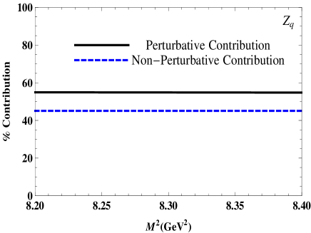
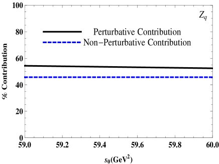
Figure 1: The perturbative and nonperturbative contributions to the sum rule as functions of $M^{2}$ at an average $s_{0}$ (left panel), and as functions of $s_{0}$ at an average $M^{2}$ (right panel).

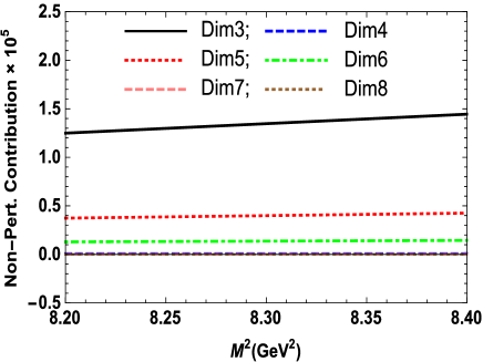
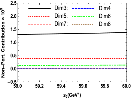
Figure 2: Contributions to the sum rule arising from the nonperturbative operators of different dimensions are shown as functions of the Borel parameter at an average value of $s_{0}$ (left panel), and as functions of the threshold parameter $s_{0}$ at an average $M^{2}$ (right panel).

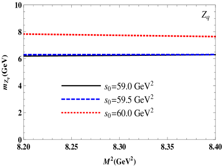
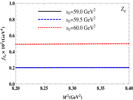
Figure 3: The mass (left panel) and meson-current coupling (right panel) as functions of the Borel parameter $M^{2}$ at fixed values of the continuum threshold $s_{0}$.

The sum rules contain the parameters, which are necessary for numerical computations: Their numerical values are collected in Table 1. The quark and gluon condensates are well known, therefore we utilize their standard values. The Table 1 contains also $B_{c}$, $\rho$ and $\phi$ mesons’ masses (see, Ref. Olive:2016xmw ) and decay constants, which will serve as input parameters when computing the strong couplings and decay widths. It is worth noting that for $f_{\rho}$, $\phi$ and $f_{B_{c}}$ we use the sum rule estimations from Refs. Ball:2007zt ; Baker:2013mwa .

The sum rules Eqs. (11) and (12) contain also two parameters $s_{0}$ and $M^{2}$, choices of which are decisive to extract reliable estimations for the quantities under question. The continuum threshold $s_{0}$ determines a boundary that dissects ground state contribution from ones due to excited resonances and continuum. It depends on the energy of the first excited state corresponding to the ground state hadron. The continuum threshold $s_{0}$ can also be found from analysis of the pole to total contribution ratio. The analysis done in the case of the tetraquark $Z_{q}$ allows us to fix a working interval for $s_{0}$ as

$$59\ \mathrm{GeV}^{2}\leq s_{0}\leq 60\ \mathrm{GeV}^{2}.$$ (13)

The Borel parameter $M^{2}$ has also to satisfy well-known requirements. Namely, convergence of OPE and exceeding of the perturbative contribution over the nonperturbative one fixes a lower bound of the allowed values of $M^{2}$. The upper limit of the Borel parameter is determined to achieve the largest possible pole contribution to the sum rule. These constraints lead to the following working window for $M^{2}$

$$8.2\ \mathrm{GeV}^{2}\leq M^{2}\leq 8.4\ \mathrm{GeV}^{2}.$$ (14)

In Figs. 1 and 2 we graphically demonstrate some stages in extracting of the working regions for these parameters. Thus, in Fig. 1 the perturbative and nonperturbative contributions to the sum rule in the chosen regions for $s_{0}$ and $M^{2}$ are depicted. The convergence of OPE can be seen by inspecting Fig. 2, where the effects of the operators of the different dimensions are plotted. By varying the parameters $s_{0}$ and $M^{2}$ within their working ranges we find, that the pole contribution to the mass sum rule amounts to $\sim 65\%$ of the result.

The final results for the mass and meson-current coupling of the $Z_{q}$ state are drawn in Fig. 3 and collected in Table 2. As is seen from Fig. 3, the quantities extracted from the sum rules demonstrate a mild dependence on $M^{2}$, whereas effects of $s_{0}$ on them are sizable. The uncertainties generated by the parameters $s_{0}$ and $M^{2}$ are main sources of errors, which are inherent part of sum rule computations and equal up to $30\%$ of the whole integral.

The mass and meson-current coupling of the $Z_{s}$ state can be obtained from the similar calculations, the difference being only in terms $\sim m_{s}$ kept in the spectral density, whereas in $Z_{q}$ calculations we set $m_{q}=0$. These modifications and also replacement $\mathcal{M}\Rightarrow m_{b}+m_{c}+2m_{s}$ in the integrals result in shifting of the working ranges of the parameters $s_{0}$ and $M^{2}$ towards slightly larger values, which now read

$$60\ \mathrm{GeV}^{2}\leq s_{0}\leq 61\ \mathrm{GeV}^{2},$$

$$8.4\ \mathrm{GeV}^{2}\leq M^{2}\leq 8.6\ \mathrm{GeV}^{2}.$$ (15)

Predictions for $m_{Z_{s}}$ and $f_{Z_{s}}$ obtained using $s_{0}$ and $M^{2}$ from Eq. (15) are also written down in Table 2.

Mass, m.-c. coupling	Results
$m_{Z_{q}}$	$(7.06\pm 0.74)~{}\mathrm{GeV}$
$f_{Z_{q}}$	$(0.33\pm 0.11)\cdot 10^{-2}~{}\mathrm{GeV}^{4}$
$m_{Z_{s}}$	$(7.30\pm 0.76)~{}\mathrm{GeV}$
$f_{Z_{s}}$	$(0.63\pm 0.19)10^{-2}~{}\mathrm{GeV}^{4}$

Table 2: The sum rule results for the masses and meson-current couplings of the axial-vector $Z_{q}$ and $Z_{s}$ states.

III $Z_{q}\rightarrow B_{c}\rho$ and $Z_{s}\rightarrow B_{c}\phi$ decays

In this section we investigate the strong decays of the exotic axial-vector $Z_{q(s)}$ states, and calculate widths of their main decay modes, which, in accordance with results of Sec. II, are kinematically allowed.

One can see, that the quantum numbers, quark content and mass of the $Z_{q}$ tetraquark make the process $Z_{q}\rightarrow B_{c}\rho$ its preferable decay mode. The $Z_{s}$ state may decay to $B_{c}$ and $\phi$ mesons. It is worth noting that, due to the $\rho-\omega$ and $\omega-\phi$ mixing, the processes $Z_{q}\rightarrow B_{c}\omega$ and $Z_{s}\rightarrow B_{c}\omega$ are also among their kinematically allowed decay channels. But because, for example, $\phi$ and $\omega$ mesons are almost pure $\overline{s}s$ and $\left(\overline{u}u+\overline{d}d\right)/\sqrt{2}$ states the $Z_{s}\rightarrow B_{c}\omega$ process is unessential provided the mass of $Z_{s}$ allows its decay to $\phi$ meson: Alternative channels with $\omega$ may play an important role in exploration of the tetraquark states containing $\bar{s}s$ pair, if their masses are not enough to create $\phi$ meson.

We are going to carry out a required analysis and write down all expressions necessary to find the $Z_{q}\rightarrow B_{c}\rho$ decay’s width. After rather trivial replacements in corresponding formulas and input parameters, the same calculations can easily be repeated for the $Z_{s}\rightarrow B_{c}\phi$ decay.

As first step we have to compute the coupling $g_{Z_{q}B_{c}\rho}$, which describes the strong interaction in the vertex $Z_{q}B_{c}\rho$, and can be extracted from the QCD sum rule. To this end, we explore the correlation function

$$\Pi_{\mu}(p,q)=i\int d^{4}xe^{ipx}\langle\rho(q)|\mathcal{T}\{J^{B_{c}}(x)J_{\mu}^{{\dagger}}(0)\}|0\rangle,$$ (16)

where $J^{B_{c}}(x)$ is the interpolating current of the $B_{c}$ meson: It is defined in the form

$$J^{B_{c}}(x)=i\overline{b}_{l}(x)\gamma_{5}c_{l}(x).$$ (17)

The correlation function in Eq. (16) is introduced in the form, which implies usage of the light-cone sum rule method. Indeed, $\Pi_{\mu}(p,q)$ will be computed employing QCD sum rule on the light-cone by using a technique of the soft-meson approximation.

In terms of the physical parameters of the involved particles and coupling $g_{Z_{q}B_{c}\rho}$ the function $\Pi_{\mu}(p,q)$ has a simple form and generates the phenomenological side of the sum rule. Namely,

$$\Pi_{\mu}^{\mathrm{Phys}}(p,q) = \frac{\langle 0|J^{B_{c}}|B_{c}\left(p\right)\rangle}{p^{2}-m_{B_{c}}^{2}}\langle B_{c}\left(p\right)\rho(q)|Z_{q}(p^{\prime})\rangle$$ (18)

$$\times\frac{\langle Z_{q}(p^{\prime})|J_{\mu}^{\dagger}|0\rangle}{p^{\prime 2}-m_{Z}^{2}}+\ldots,$$

where $p$, $q$ and $p^{\prime}=p+q$ are the momenta of $B_{c}$, $\rho$ and $Z_{q}$ particles, respectively. The term presented above is the contribution of the ground state: the dots stand for effects of the higher resonances and continuum states.

We introduce the $B_{c}$ meson matrix element

$$\langle 0|J^{B_{c}}|B_{c}\left(p\right)\rangle=\frac{f_{B_{c}}m_{B_{c}}^{2}}{m_{b}+m_{c}}$$

where $m_{B_{c}}$ and $f_{B_{c}}$ are the mass and decay constant of the $B_{c}$ meson, and also the matrix element corresponding to the vertex

$$\langle B_{c}\left(p\right)\rho(q)|Z_{q}(p^{\prime})\rangle = g_{Z_{q}B_{c}\rho}\left[\left(q\cdot\varepsilon^{\prime}\right)\left(p^{\prime}\cdot\varepsilon^{\ast}\right)\right.$$ (19)

$$\left.-\left(q\cdot p^{\prime}\right)\left(\varepsilon^{\ast}\cdot\varepsilon^{\prime}\right)\right].$$

Then the ground state term in the correlation function can be easily found, as:

$$\Pi_{\mu}^{\mathrm{Phys}}(p,q)=\frac{f_{B_{c}}f_{Z}m_{Z}m_{B_{c}}^{2}g_{Z_{q}B_{c}\rho}}{\left(p^{\prime 2}-m_{Z}^{2}\right)\left(p^{2}-m_{B_{c}}^{2}\right)(m_{b}+m_{c})}$$

$$\times\left(\frac{m_{Z}^{2}-m_{B_{c}}^{2}}{2}\varepsilon_{\mu}^{\ast}-p^{\prime}\cdot\varepsilon^{\ast}q_{\mu}\right)+\ldots.$$ (20)

Strong vertices of a tetraquark with two conventional mesons differ from vertices containing only ordinary mesons. The reason here is very simple: the tetraquark $Z_{q}$ is a state composed of four valence quarks, therefore the expansion of the non-local correlation function $\Pi_{\mu}(p,q)$ leads to the expression, which instead of distribution amplitudes of $\rho$ meson depends on its local matrix elements (of course, same arguments are valid for $Z_{s}$, as well). Then, the conservation of the four-momentum at the vertex $Z_{q}B_{c}\rho$ equals $q$ to zero. In other words, within the light-cone sum rule method the momentum of $\rho$ meson should be equal to zero in our case. In vertices of ordinary hadrons four-momenta of all involved particles can take nonzero values. The soft-meson approximation corresponds to a situation when $q=0$. Calculations of the same strong couplings within the full light-cone sum rule method and in the soft-meson approximation demonstrated that the difference between results extracted using these two approaches is numerically small (for detailed discussion, see Ref. Braun:1995 ).

In the soft limit $p=p^{\prime}$, only the term that survives in Eq. (20) is $\sim\varepsilon_{\mu}^{\ast}$. The invariant function $\Pi^{\mathrm{Phys}}(p^{2})$ corresponding to this structure depends on the variable $p^{2}$, and is given as

$$\Pi^{\mathrm{Phys}}(p^{2})=\frac{f_{B_{c}}f_{Z}m_{Z}m_{B_{c}}^{2}g_{Z_{s}B_{c}\eta}}{2\left(p^{2}-m^{2}\right)^{2}(m_{b}+m_{c})}$$

$$\times\left(m_{Z}^{2}-m_{B_{c}}^{2}\right)+\ldots,$$ (21)

where $m^{2}=\left(m_{Z}^{2}+m_{B_{c}}^{2}\right)/2.$

In the soft-meson approximation we additionally apply the operator

$$\left(1-M^{2}\frac{d}{dM^{2}}\right)M^{2}e^{m^{2}/M^{2}},$$ (22)

to both sides of the sum rule. The last operation is required to remove all unsuppressed contributions existing in the physical side of the sum rule in the soft-meson limit (see, Ref. Ioffe:1983ju ).

The second component of the sum rule, i.e. QCD expression for the correlation function $\Pi^{\mathrm{QCD}}_{\mu}(p,q)$ is calculated employing the quark propagators and shown below

$$\Pi_{\mu}^{\mathrm{QCD}}(p,q)=-i\int d^{4}xe^{ipx}\left\{\left[\gamma_{5}\widetilde{S}_{c}^{ib}(x){}\gamma_{5}\right.\right.$$

$$\left.\times\widetilde{S}_{b}^{bi}(-x){}\gamma_{\mu}\right]_{\alpha\beta}\langle\rho(q)|\overline{q}_{\alpha}^{a}q_{\beta}^{a}|0\rangle$$

$$\left.+\left[\gamma_{5}\widetilde{S}_{c}^{ib}(x)\gamma_{5}\widetilde{S}_{b}^{ai}(-x){}\gamma_{\mu}\right]_{\alpha\beta}\langle\rho(q)|\overline{s}_{\alpha}^{a}s_{\beta}^{b}|0\rangle\right\},$$ (23)

with $\alpha$ and $\beta$ being the spinor indices.

We continue our calculations by employing the expansion

$$\overline{q}_{\alpha}^{a}q_{\beta}^{b}\rightarrow\frac{1}{4}\Gamma_{\beta\alpha}^{j}\left(\overline{q}^{a}\Gamma^{j}q^{b}\right),$$ (24)

where $\Gamma^{j}=1,\ \gamma_{5},\ \gamma_{\mu},\ i\gamma_{5}\gamma_{\mu},\ \sigma_{\mu\nu}/\sqrt{2}$ is the full set of Dirac matrices, and carry out the color summation.

Prescriptions to perform summation over color indices, as well as procedures to calculate resulting integrals and extract the imaginary part of the correlation function $\Pi_{\mu}^{\mathrm{QCD}}(p,q)$ were numerously presented in our previous works Refs. Agaev:2016dev ; Agaev:2016ijz ; Agaev:2016lkl ; Agaev:2016urs . Therefore, here we skip further details, and provide the $\rho$ meson local matrix elements that in the soft limit contribute to the spectral density, as well as, final formulas for the spectral density $\rho_{c}(s)$.

Analysis demonstrates that in the soft limit only the matrix elements

$$\langle 0|\overline{q}\gamma_{\mu}q|\rho^{0}(p)\rangle=\frac{1}{\sqrt{2}}f_{\rho}m_{\rho}\varepsilon_{\mu},$$ (25)

and

$$\langle 0|\overline{q}g\widetilde{G}_{\mu\nu}\gamma_{\nu}\gamma_{5}q|\rho^{0}(p)\rangle=\frac{1}{\sqrt{2}}f_{\rho}m_{\rho}^{3}\zeta_{4\rho}\varepsilon_{\mu},$$ (26)

are involved into computations, where $q$ denotes one of the $u$ or $d$ quarks. The matrix elements depend on the $\rho$ meson mass $m_{\rho}$ and decay constant $f_{\rho}$. The twist-4 matrix element in Eq. (26), as a factor, contains also the parameter $\zeta_{4\rho}$. Its numerical value was extracted at the scale $\mu=1\ \mathrm{GeV}$ from the sum rule calculations in Ref. Ball:2007zt and equals to

$$\zeta_{4\rho}=0.07\pm 0.03.$$

The final expression of the spectral density has the form

$$\rho_{c}(s)=\frac{f_{\rho}m_{\rho}}{24\sqrt{2}}\left[F^{\mathrm{pert.}}(s)+F^{\mathrm{n.-pert.}}(s)\right].$$ (27)

Here $F^{\mathrm{pert.}}(s)$ is the perturbative contribution to $\rho_{c}(s)$

$$F^{\mathrm{pert.}}(s)=\frac{1}{\pi^{2}s^{2}}\left\{\left[s^{2}+s\left(m_{b}^{2}+6m_{b}m_{c}+m_{c}^{2}\right)\right.\right.$$

$$\left.\left.-2(m_{b}^{2}-m_{c}^{2})^{2}\right]\right\}\sqrt{\left(s+m_{b}^{2}-m_{c}^{2}\right)^{2}-4m_{b}^{2}s},$$ (28)

whereas by $F^{\mathrm{n.-pert.}}(s)$ we denote its nonperturbative component. The function $F^{\mathrm{n.-pert.}}(s)$ is the sum of the terms

$$F^{\mathrm{n.-pert.}}(s)=F_{G}^{\mathrm{n.-pert.}}(s)+\Big{\langle}\frac{\alpha_{s}G^{2}}{\pi}\Big{\rangle}\int_{0}^{1}f_{g_{s}^{2}G^{2}}(z,s)dz$$

$$+\Big{\langle}g_{s}^{3}G^{3}\Big{\rangle}\int_{0}^{1}f_{g_{s}^{3}G^{3}}(z,s)dz$$

$$+\Big{\langle}\frac{\alpha_{s}G^{2}}{\pi}\Big{\rangle}^{2}\int_{0}^{1}f_{(g_{s}^{2}G^{2})^{2}}(z,s)dz.$$ (29)

Here $F_{G}^{\mathrm{n.-pert.}}(s)$ appears from integration of the perturbative component of one heavy quark propagator with the term $\sim G$ from another one. It can be expressed using the matrix element given by Eq. (26) and has a rather simple form

$$F_{G}^{\mathrm{n.-pert.}}(s)=\frac{3m_{\rho}^{2}\zeta_{4\rho}}{2\pi^{2}s}\sqrt{\left(s+m_{b}^{2}-m_{c}^{2}\right)^{2}-4m_{b}^{2}s}.$$ (30)

The nonperturbative factors in front of the integrals, and subscripts of the functions clearly indicate the origin of the remaining terms. In fact, the functions $f_{g_{s}^{2}G^{2}}$, $f_{g_{s}^{3}G^{3}}$ are due to products of $\sim g_{s}^{2}G^{2}$ and $\sim g_{s}^{3}G^{3}$ terms with the perturbative component of another propagator, whereas $f_{(g_{s}^{2}G^{2})^{2}}$ comes from integrals obtained using $\sim g_{s}^{2}G^{2}$ components of $b$ and $c$ quarks’ propagators. These terms are four, six and eight dimensional nonperturbative contributions to the spectral density $\rho_{c}(s)$, respectively. Their explicit forms are presented below:

$$f_{g_{s}^{2}G^{2}}(z,s)=\frac{1}{12z^{2}(z-1)^{2}}\left\{54(1-z)z^{2}\delta(s-\Phi)+\left[8m_{b}^{2}(z-1)^{3}+z^{2}\left(27s(1-z)-8m_{b}^{2}z\right)\right.\right.$$

$$\left.\left.+2m_{b}m_{c}\left(4+15z+12z^{2}\right)\right]\delta^{(1)}(s-\Phi)-4s\left[m_{b}^{2}(1-z)^{3}+m_{b}m_{c}z(1-z)-m_{c}^{2}z^{3}\right]\delta^{(2)}(s-\Phi)\right\},$$ (31)

$$f_{g_{s}^{3}G^{3}}(z,s)=\frac{1}{15\cdot 2^{6}z^{5}(z-1)^{5}}\left\{-12z^{2}(z-1)^{2}\left[3m_{b}^{2}(z-1)^{5}+3m_{b}m_{c}((1-z)^{5}+z^{5})+z\left(-3m_{c}^{2}z^{4}\right.\right.\right.$$

$$\left.\left.+s\left(1-8z+25z^{2}-40z^{3}+33z^{4}-11z^{5}\right)\right)\right]\delta^{(2)}(s-\Phi)+2z(z-1)\left[m_{b}^{2}(z-1)^{5}\left(7m_{b}^{2}-4m_{b}m_{c}-9sz(2z-1)\right)\right.$$

$$\left.+2m_{b}m_{c}z^{2}\left(2m_{c}^{2}z^{3}-9s(z-1)^{2}(1-3z+3z^{2})\right)+z^{3}\left(-7m_{c}^{4}z^{2}+9sm_{c}^{2}z^{2}(1-3z+2z^{2})+2s^{2}(z-1)^{3}(2-7z+7z^{2})\right)\right]$$

$$\times\delta^{(3)}(s-\Phi)+\left[-2m_{b}^{5}m_{c}(z-1)^{5}+7m_{b}^{4}sz(z-1)^{6}-4m_{b}^{3}m_{c}sz^{2}(z-1)^{5}-6m_{b}^{2}s^{2}z^{3}(z-1)^{6}+2m_{b}m_{c}z^{4}\right.$$

$$\left.\left.\times\left(-3s^{2}(z-1)^{4}+m_{c}^{4}z+2m_{c}^{2}sz(z-1)^{2}\right)+s(z-1)z^{5}\left(s^{2}(z-1)^{4}-7m_{c}^{4}z+6m_{c}^{2}sz(z-1)^{2}\right)\right]\delta^{(4)}(s-\Phi)\right\},$$ (32)

$$f_{(g_{s}^{2}G^{2})^{2}}(z,s)=\frac{m_{b}m_{c}}{54z^{2}(z-1)^{2}}\left\{2\left[m_{b}m_{c}-s(1-3z+3z^{2})\right]\delta^{(4)}(s-\Phi)+s[m_{b}m_{c}+s(1-z)z]\delta^{(5)}(s-\Phi)\right\},$$ (33)

where,

$$\delta^{(n)}(s-\Phi)=\frac{d^{n}}{ds^{n}}\delta(s-\Phi),$$

with $\Phi$ being defined as

$$\Phi=\frac{m_{b}^{2}(1-z)+m_{c}^{2}z}{z(1-z)}.$$

The final sum rule to evaluate the strong coupling reads

$$g_{Z_{q}B_{c}\rho}=\frac{2(m_{b}+m_{c})}{f_{B_{c}}f_{Z}m_{Z}m_{B_{c}}^{2}(m_{Z}^{2}-m_{B_{c}}^{2})}\left(1-M^{2}\frac{d}{dM^{2}}\right)$$

$$\times M^{2}\int_{(m_{b}+m_{c})^{2}}^{s_{0}}dse^{(m^{2}-s)/M^{2}}\rho_{c}(s).$$ (34)

To calculate the width of the decay $Z_{q}\rightarrow B_{c}\rho$ we use the expression,

$$\Gamma\left(Z_{q}\rightarrow B_{c}\rho\right)=\frac{g_{Z_{q}B_{c}\rho}^{2}m_{\rho}^{2}}{24\pi}\lambda\left(m_{Z},\ m_{B_{c}},m_{\rho}\right)$$

$$\times\left[3+\frac{2\lambda^{2}\left(m_{Z_{q}},\ m_{B_{c}},m_{\rho}\right)}{m_{\rho}^{2}}\right],$$ (35)

where

$$\lambda(a,\ b,\ c)=\frac{\sqrt{a^{4}+b^{4}+c^{4}-2\left(a^{2}b^{2}+a^{2}c^{2}+b^{2}c^{2}\right)}}{2a}.$$

Parameters necessary for numerical calculations of the strong coupling $g_{Z_{q}B_{c}\rho}$ and $\Gamma\left(Z_{q}\rightarrow B_{c}\rho\right)$ are listed in Table 1.

Strong couplings, Widths	Predictions
$g_{Z_{q}B_{c}\rho}$	$(5.31\pm 1.25)$ $\mathrm{GeV}^{-1}$
$g_{Z_{s}B_{c}\phi}$	$(6.42\pm 1.52)$ $\mathrm{GeV}^{-1}$
$\Gamma(Z_{q}\to B_{c}\rho)$	$(80\pm 32)$ $\mathrm{MeV}$
$\Gamma(Z_{s}\to B_{c}\phi)$	$(168\pm 68)$ $\mathrm{MeV}$

Table 3: The strong couplings and decay widths of the $Z_{q}$ and $Z_{s}$ tetraquarks.

The investigation carried out in accordance with standard requirements of the sum rule calculations allows us to determine the ranges for $s_{0}$ and $M^{2}$. For example, the pole contribution to the sum rule amounts to $\sim 48-60\%$ of the total result, as is seen from Fig. 4. Other constraints, i.e. convergence of OPE, prevalence of the perturbative contribution have been checked, as well. Summing up the performed analysis we fix the interval for the continuum threshold $s_{0}$ as in the mass calculations (see, Eq. (13)), whereas for the Borel parameter we obtain

$$8\ \mathrm{GeV}^{2}\leq M^{2}\leq 9\ \mathrm{GeV}^{2},$$ (36)

which is wider than the corresponding window in the mass sum rule.

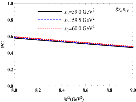
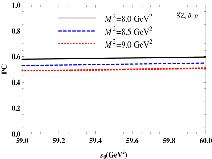
Figure 4: The pole contribution in the $g_{Z_{q}B_{c}\rho}$ coupling sum rule calculations as a function of the Borel parameter $M^{2}$ at fixed $s_{0}$ (left panel), and as a function of the threshold $s_{0}$ at fixed values of $M^{2}$ (right panel).

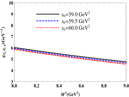
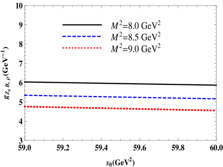
Figure 5: The strong coupling $g_{Z_{q}B_{c}\rho}$ as a function of the Borel parameter $M^{2}$ at fixed $s_{0}$ (left panel), and as a function of the threshold $s_{0}$ at fixed values of $M^{2}$ (right panel).

In Fig. 5 we provide our final results and depict the strong coupling $g_{Z_{q}B_{c}\rho}$ as the function of the Borel parameter (at fixed $s_{0}$) and as the function of the continuum threshold (at fixed $M^{2}$). The dependence of the strong coupling on these parameters has a traditional form, and systematic errors of the calculations are within reasonable limits.

The decay $Z_{s}\rightarrow B_{c}\phi$ can be considered in analogous manner: One only needs to write down in the relevant expressions the parameters of the $\phi$ meson. Thus, the matrix elements of the $\phi$ meson that take part in forming of the spectral density are

$$\langle 0|\overline{s}\gamma_{\mu}s|\phi(p)\rangle = f_{\phi}m_{\phi}\varepsilon_{\mu},$$

$$\langle 0|\overline{s}g\widetilde{G}_{\mu\nu}\gamma_{\nu}\gamma_{5}s|\phi(p)\rangle = f_{\phi}m_{\phi}^{3}\zeta_{4\phi}\varepsilon_{\mu},$$

where the twist-4 parameter

$$\zeta_{4\phi}=0.00\pm 0.02$$

was estimated and found compatible with zero in Ref. Ball:2007zt .

In calculations of the coupling $g_{Z_{s}B_{c}\phi}$ the working regions for the Borel parameter and continuum threshold are fixed in the form:

$$60\ \mathrm{GeV}^{2}\leq s_{0}\leq 61\ \mathrm{GeV}^{2},$$

$$8.2\ \mathrm{GeV}^{2}\leq M^{2}\leq 9.2\ \mathrm{GeV}^{2}.$$ (37)

Our results for the strong couplings and widths of the decay modes studied in this work are collected in Table 3.

IV Discussion and concluding remarks

In the present work we have calculated the parameters of the open charm-bottom axial-vector tetraquark states $Z_{q}$ and $Z_{s}$ within QCD sum rule method. Their masses and meson-current couplings have been obtained using the two-point sum rule method. In these calculations for $Z_{q}$ and $Z_{s}$ we have used the symmetric in color indices interpolating currents by assuming that they are ground states in corresponding tetraquark multiplets. Indeed, one can anticipate that $Z_{q}$ and $Z_{s}$ are the axial-vector components of the $1S$ diquark-antidiquark $[cq][\bar{b}\bar{q}]$ and $[cs][\bar{b}\bar{s}]$ multiplets, respectively.

During last years some progress was archived in investigation of the $[cq][\bar{c}\bar{q}]$ and $[cs][\bar{c}\bar{s}]$ multiplets, and classification of the observed hidden-charm tetraquarks as their possible members (see, Refs. Maiani:2014 ; Maiani:2016wlq ). Thus, within the ”type-II” model elaborated in these works, the authors not only identified the multiplet levels with discovered tetraquarks, but also estimated masses of the states, which had not yet been observed. This model is founded on some assumptions about a nature of inter-quark and inter-diquark interactions, and considers spin-spin interactions within diquarks as decisive source of splitting inside of the multiplet.

The information useful for our purposes is accumulated in the axial-vector sector of these multiplets. The axial-vector $J^{PC}=1^{++}$ particle in the ground-state $[cq][\bar{c}\bar{q}]$ multiplet was identified with the well-known $X(3872)$ resonance. The similar analysis carried out for the multiplet of $[cs][\bar{c}\bar{s}]$ states demonstrated that its $J^{PC}=1^{++}$ level may be considered as $X(4140)$. The mass difference of the axial-vector resonances belonging to $"q"$ and $"s"$ hidden-charm multiplets is

$$X(4140)-X(3872)\approx 270\,\mathrm{MeV}.$$ (38)

In the present work we have evaluated masses of the axial-vector states from the $[cq][\bar{b}\bar{q}]$ and $[cs][\bar{b}\bar{s}]$ multiplets. The mass shift between these multiplets

$$m_{Z_{s}}-m_{Z_{q}}\approx 240\,\mathrm{MeV},$$ (39)

is in nice agreement with Eq. (38).

Another question to be addressed here is connected with masses of excited states, which in sum rule calculations determine continuum threshold $s_{0}$. We have found that for $[cq][\bar{b}\bar{q}]$ and $[cs][\bar{b}\bar{s}]$ multiplets sum rule calculations fix the lower bounds of the parameter $s_{0}$ as $s_{0}=59\,\,\mathrm{GeV^{2}}$ and $s_{0}=60\,\,\mathrm{GeV^{2}}$, respectively. This means that sum rule has placed a first excited state to position $\sqrt{s}_{0}$. In order to estimate a gap between the excited and ground states we invoke $\sqrt{s}_{0}$ and central values of $Z_{q}$ and $Z_{s}$ masses. Then, it is not difficult to see, that for $[cq][\bar{b}\bar{q}]$ type tetraquarks, it equals to

$$\sqrt{s}_{0}\,\mathrm{GeV}-7.06\,\mathrm{GeV}\approx 0.62\,\mathrm{GeV},$$ (40)

whereas for the $[cs][\bar{b}\bar{s}]$ one gets

$$\sqrt{s}_{0}\,\mathrm{GeV}-7.30\,\mathrm{GeV}\approx 0.45\,\mathrm{GeV}.$$ (41)

The masses of $1S$ and $2S$ states with $J^{PC}=1^{+-}$ from the $[cq][\bar{c}\bar{q}^{\prime}]$ multiplet were calculated by means of the two-point sum rule method in Ref. Wang:2014vha . The ground-state level $1S$ was identified with the resonance $Z_{c}(3900)$, whereas the resonance $Z(4430)$ was included into a multiplet of the excited $2S$ states. If this assignment is correct, then the experimental data provides the mass difference between the ground and first radially excited states, which is equal to $530\,\mathrm{MeV}$. Results of the calculations led to predictions $M_{Z_{c}(3900)}=3.91^{+21}_{-17}\,\mathrm{GeV}$ and $M_{Z_{c}(4430)}=4.51^{+17}_{-09}\,\mathrm{GeV}$, and to the mass difference $\sim 600\,\mathrm{MeV}$.

The $1S$ and $2S$ multiplets of $[cs][\bar{c}\bar{s}]$ tetraquarks were explored in the context of the ”type-II” model in Ref. Maiani:2016wlq . For the axial-vector levels $J^{PC}=1^{++}$ named there as $X$ states, the $2S-1S$ gap is $4600\,\mathrm{MeV}-4140\,\mathrm{MeV}=460\,\mathrm{MeV}$, and for the particles $X^{(1)}$ and $X^{(2)}$ with the quantum numbers $J^{PC}=1^{+-}$ one gets $4600\,\mathrm{MeV}-4140\,\mathrm{MeV}=460\,\mathrm{MeV}$ and $4700\,\mathrm{MeV}-4274\,\mathrm{MeV}=426\,\mathrm{MeV}$, respectively. Comparison of these results with ones given by Eqs. (40) and (41) can be considered as confirmation of a self-consistent character of the performed analysis.

In the framework of QCD two-point sum rule approach masses of the open charm-bottom diquark-antidiquark states were previously calculated in Ref. Chen:2013aba . For masses of the axial-vector tetqaruarks $Z_{q}$ and $Z_{s}$ the authors found:

$$m_{Z_{q}}=7.10\pm 0.09\pm 0.06\pm 0.01\,\,\mathrm{GeV},$$ (42)

and

$$m_{Z_{s}}=7.11\pm 0.08\pm 0.05\pm 0.03\,\,\mathrm{GeV}.$$ (43)

These predictions were extracted by using the parameter $s_{0}=(55\pm 2)\,\,\mathrm{GeV}^{2}$ in calculations of $m_{Z_{q}}$ and $m_{Z_{s}}$, and $M^{2}=(7.9-8.2)\,\,\mathrm{GeV}^{2}$ and $M^{2}=(6.7-7.9)\,\,\mathrm{GeV}^{2}$ for $"q"$ and $"s"$ states, respectively. It is seen, that mass differences $m_{Z_{s}}-m_{Z_{q}}\approx 10\,\,\mathrm{MeV}$ and $\sqrt{s}_{0}-m_{Z_{q}}\approx\sqrt{s}_{0}-m_{Z_{s}}\approx 180\,\,\mathrm{MeV}$ can be neither included into $"q"-"s"$ mass-hierarchy scheme of the ground state tetraquarks nor accepted as giving correct mass shift between $1S$ and $2S$ multiplets. Our results for $m_{Z_{q}}$ and $m_{Z_{s}}$, if differences are ignored in chosen windows for the parameters $s_{0}$ and $M^{2}$, within theoretical errors may be considered as being in agreement with the predictions of Ref.  Chen:2013aba . But in our case the central value of $m_{Z_{s}}$ allows the decay process $Z_{s}\to B_{c}\phi$, whereas for $m_{Z_{s}}$ from Eq. (43) it remains among kinematically forbidden channels.

We have also calculated the widths of the $Z_{q}\to B_{c}\rho$ and $Z_{s}\to B_{c}\phi$ decays, which are new results of this work. Obtained predictions for $\Gamma(Z_{q}\to B_{c}\rho)$ and $\Gamma(Z_{s}\to B_{c}\phi)$ show that $Z_{q}$ may be considered as a narrow resonance, whereas $Z_{s}$ belongs to a class of wide tetraquark states.

Investigation of the open charm-bottom axial-vector tetraquarks performed in the present work within the diquark-antidiquark picture led to quite interesting predictions. Theoretical explorations of other members of the $[cq][\bar{b}\bar{q}]$ and $[cs][\bar{b}\bar{s}]$ tetraquark multiplets, as well as their experimental studies may shed light on the nature of multi-quark hadrons.

References

- (1) H. X. Chen, W. Chen, X. Liu and S. L. Zhu, Phys. Rept. 639, 1 (2016).
- (2) H. X. Chen, W. Chen, X. Liu, Y. R. Liu and S. L. Zhu, arXiv:1609.08928 [hep-ph].
- (3) A. Esposito, A. L. Guerrieri, F. Piccinini, A. Pilloni and A. D. Polosa, Int. J. Mod. Phys. A 30, 1530002 (2015).
- (4) C. A. Meyer and E. S. Swanson, Prog. Part. Nucl. Phys. 82, 21 (2015)
- (5) S.-K. Choi et al. [Belle Collaboration], Phys. Rev. Lett. 91, 262001 (2003).
- (6) D. Acosta et al. [CDF II Collaboration] Phys. Rev. Lett. 93, 072001 (2004).
- (7) V. M. Abazov et al. [D0 Collaboration], Phys. Rev. Lett. 93, 162002 (2004).
- (8) B. Aubert et al. [BaBar Collaboration], Phys. Rev. D 71, 071103 (2005).
- (9) K. Abe et al. [Belle Collaboration], BELLE-CONF-0540, hep-ex/0505037.
- (10) B. Aubert et al. [BaBar Collaboration], Phys. Rev. Lett. 102, 132001 (2009).
- (11) T. Barnes, S. Godfrey and E. S. Swanson, Phys. Rev. D 72, 054026 (2005).
- (12) I. V. Danilkin and Y. A. Simonov, Phys. Rev. Lett. 105, 102002 (2010).
- (13) F. E. Close and P. R. Page,
- (14) N. A. Tornqvist, Phys. Lett. B 590, 209 (2004).
- (15) C. M. Zanetti, M. Nielsen and R. D. Matheus, Phys. Lett. B 702, 359 (2011).
- (16) F. K. Guo, C. Hanhart, Y. S. Kalashnikova, U. G. Meißner and A. V. Nefediev, Phys. Lett. B 742, 394 (2015).
- (17) L. Maiani, F. Piccinini, A. D. Polosa and V. Riquer, Phys. Rev. D 71, 014028 (2005).
- (18) L. Maiani, A. D. Polosa and V. Riquer, Phys. Rev. Lett. 99, 182003 (2007),
- (19) F. S. Navarra and M. Nielsen, Phys. Lett. B 639, 272 (2006).
- (20) S. Dubnicka, A. Z. Dubnickova, M. A. Ivanov and J. G. Korner, Phys. Rev. D 81, 114007 (2010).
- (21) Z. G. Wang and T. Huang, Phys. Rev. D 89, 054019 (2014).
- (22) B. Aubert et al. [BaBar Collaboration], Phys. Rev. Lett. 90, 242001 (2003).
- (23) D. Besson et al. [CLEO Collaboration], Phys. Rev. D 68, 032002 (2003) Erratum: [Phys. Rev. D 75, 119908 (2007)].
- (24) V. M. Abazov et al. [D0 Collaboration], Phys. Rev. Lett. 117, 022003 (2016).
- (25) The D0 Collaboration, D0 Note 6488-CONF, (2016).
- (26) R. Aaij et al. [LHCb Collaboration], Phys. Rev. Lett. 117, 152003 (2016).
- (27) The CMS Collaboration, CMS PAS BPH-16-002, (2016).
- (28) J. R. Zhang and M. Q. Huang, Phys. Rev. D 80, 056004 (2009).
- (29) J. R. Zhang and M. Q. Huang, Commun. Theor. Phys. 54, 1075 (2010)
- (30) W. Chen, T. G. Steele and S. L. Zhu, Phys. Rev. D 89, 054037 (2014).
- (31) S. Zouzou, B. Silvestre-Brac, C. Gignoux and J. M. Richard, Z. Phys. C 30, 457 (1986).
- (32) B. Silvestre-Brac and C. Semay, Z. Phys. C 59, 457 (1993).
- (33) D. Ebert, R. N. Faustov, V. O. Galkin and W. Lucha, Phys. Rev. D 76, 114015 (2007).
- (34) Z. F. Sun, X. Liu, M. Nielsen and S. L. Zhu, Phys. Rev. D 85, 094008 (2012)
- (35) R. M. Albuquerque, X. Liu and M. Nielsen, Phys. Lett. B 718, 492 (2012)
- (36) S. S. Agaev, K. Azizi and H. Sundu, Phys. Rev. D 95, 034008 (2017).
- (37) M. A. Shifman, A. I. Vainshtein and V. I. Zhakharov, Nucl. Phys. B 147, 385 (1979).
- (38) V. M. Braun and A. V. Kolesnichenko, Phys. Lett. B 175, 485 (1986).
- (39) V. M. Braun and Y. M. Shabelski, Sov. J. Nucl. Phys. 50, 306 (1989) [Yad. Fiz. 50, 493 (1989)].
- (40) I. I. Balitsky, D. Diakonov and A. V. Yung, Phys. Lett. B 112, 71 (1982); Z. Phys. C 33, 265 (1986).
- (41) J. Govaerts, L. J. Reinders, H. R. Rubinstein and J. Weyers, Nucl. Phys. B 258, 215 (1985);J. Govaerts, L. J. Reinders and J. Weyers, Nucl. Phys. B 262, 575 (1985).
- (42) I. I. Balitsky, V. M. Braun, A. V. Kolesnichenko, Nucl. Phys. B 312, 509 (1989).
- (43) B. L. Ioffe and A. V. Smilga, Nucl. Phys. B 232, 109 (1984).
- (44) V. M. Belyaev, V. M. Braun, A. Khodjamirian and R. Rückl, Phys. Rev. D 51, 6177 (1995).
- (45) S. S. Agaev, K. Azizi and H. Sundu, Phys. Rev. D 93, 074002 (2016).
- (46) S. S. Agaev, K. Azizi and H. Sundu, Phys. Rev. D 93, 114007 (2016).
- (47) S. S. Agaev, K. Azizi and H. Sundu, Phys. Rev. D 93, 094006 (2016).
- (48) S. S. Agaev, K. Azizi and H. Sundu, Eur. Phys. J. Plus 131, 351 (2016).
- (49) L. J. Reinders, H. Rubinstein and S. Yazaki, Phys. Rept. 127, 1 (1985).
- (50) S. S. Agaev, K. Azizi and H. Sundu, Phys. Rev. D 93, 074024 (2016).
- (51) C. Patrignani, Chin. Phys. C 40, 100001 (2016).
- (52) P. Ball, V. M. Braun and A. Lenz, JHEP 0708, 090 (2007).
- (53) M. J. Baker, J. Bordes, C. A. Dominguez, J. Penarrocha and K. Schilcher, JHEP 1407, 032 (2014).
- (54) L. Maiani, F. Piccinini, A. D. Polosa and V. Riquer, Phys. Rev. D 89, 114010 (2014).
- (55) L. Maiani, A. D. Polosa and V. Riquer, Phys. Rev. D 94, 054026, (2016).
- (56) Z. G. Wang, Commun. Theor. Phys. 63, 325 (2015).