WU-HEP-17-03 KIAS-P17014 Brane-localized masses in magnetic compactifications

1 Introduction

The standard model (SM) of particle physics has been verified by the discovery of the final puzzle piece—i.e., the Higgs boson—in 2012 [1, 2]. It is well known that the SM can explain almost all of the phenomena around the electroweak scale ($\sim 100$ GeV) with great accuracy. However, extensions beyond the SM are required, due to several theoretical difficulties which appear inevitably in the SM, e.g., the flavor puzzle, the lack of a dark matter candidate, the gauge hierarchy problem, and so forth.

Among such extensions beyond the SM, extra dimensions have been studied from a phenomenological point of view. Indeed, the geometry of the compactified hidden directions determines phenomenological properties in the four-dimensional (4D) low-energy effective theory (LEET). For example, it is known that some extra-dimensional properties such as Kaluza-Klein (KK) wave functions reflect information on the extra-dimensional topologies. In particular, localization of the lowest wave function(s) among the KK-decomposed modes significantly affects the LEET obtained after dimensional reduction. Indeed, many phenomenological models accompanying localization of the KK-expanded modes have been proposed and investigated. For example, overlap integrations of KK wave functions are used to realize a huge hierarchy in Yukawa coupling constants [3], where differences in the degrees of overlapping lead to the hierarchy in the eigenvalues of the Yukawa matrix. Similarly, such an overlapping of KK wave functions can provide the Froggatt-Nielsen mass matrix textures [4], their Gaussian-extended version [5], and so on. For such a reason, model builders interested in extra dimensions are intrigued by the localization of particle profiles in extra directions as a way to realize a huge hierarchy in a natural way.

On the other hand, when we address orbifold compactifications, an interesting feature is found, which is useful for concrete model constructions: the existence of orbifold fixed point(s). Model builders have added desirable terms on the orbifold fixed points to derive necessary structures and/or to conquer problems that are more difficult in the bulk part of extra dimensions. For example, the authors of Ref. [6] pointed out that the Yukawa couplings can be introduced on the $S_{1}/Z_{2}$ orbifold fixed points, although Yukawa interactions are prohibited on the bulk of $S_{1}/Z_{2}$. There are other uses of fixed points. In some papers, model builders have introduced brane-localized mass term(s) on the fixed points in order to uplift dangerous massless (or very light) particles for consistent model constructions. In Refs. [7, 8], brane-localized mass terms on the fixed points of the toroidal orbifold $T^{2}/Z_{2}$ were investigated and it was declared that a massless zero mode can become massive via effects of the brane-localized mass.

Recently, several groups have eagerly studied systems on magnetized backgrounds based on toroidal extra dimensions and their orbifolded versions [9, 10, 11, 12, 13, 14, 15, 16, 17, 18, 19, 20]. This is because magnetic fluxes play important roles in constructing phenomenological models [23]. Indeed, the presence of magnetic fluxes leads to the multiplicity of the lowest KK modes, where such an emergence of the multiple lowest modes is considered as a spontaneous generation of a family replication in LEET. Also, specific configurations of the magnetic fluxes penetrating extra dimensions break supersymmetry, (see e.g., Ref. [5]).

In this paper, we examine the situation where the two phenomenology fascinating ideas—namely, a magnetized background and a mass term localized on an orbifold fixed point—are taken into account simultaneously. Our major motivation for focusing on this configuration is as follows. A possible problem in realizing family structures when using the magnetic fluxes is that extra massless modes emerge in some concrete models. Introducing brane-localized mass terms may help such situations by making some of the light particles decoupled, which can be expected. Also, after the perturbation by the insertion of mass terms on fixed points, particle profiles are changed through the rediagonalization of a perturbed KK mass matrix, where some part of the mass spectrum may be unchanged.

This paper is organized as follows. In Sec. 2, we briefly review the KK decompositions for the six-dimensional (6D) scalar and spinor fields on a magnetized two-dimensional torus, and show that the KK-expanding wave functions are described by the Jacobi theta function and the Hermite polynomials on the basic magnetic background. Then, we focus on the $Z_{2}$-orbifolded situation of a two-dimensional torus with magnetic fluxes, where important properties of the $Z_{2}$ eigenmodes are shown. In Sec. 3, we investigate effects on the KK mass spectra after taking care of effects from brane-localized mass(es), where the forms of eigenvalues and eigenvectors after the perturbation are investigated theoretically. Subsequently, in Sec. 4 we directly explore deformations of the profile of KK particles (in the correct mass eigenbases under the brane-localized mass terms) through numerical calculations. In Sec. 5, we comment on the cutoff dependence of the KK mass eigenvalues. Section 6 is devoted to a conclusion and discussion. In Appendix A, we summarize our notation for 6D gamma matrices. In Appendix B, we provide a discussion on the situation with multiple brane-localized mass terms.

2 Brief review of bulk wave functions

In this section, we briefly review the wave functions of KK modes on a magnetized background, based on Refs. [23, 24, 25, 15].

2.1 Flux background

We consider the two actions of the 6D gauge theory on the 4D Minkowski spacetime times two-dimensional torus $T^{2}$ with a 6D Weyl spinor ($\Psi$) or a 6D complex scalar ($\Phi$), e.g.,

$$S_{\rm Weyl} =\int d^{4}x\int_{T^{2}}d^{2}z\,\{i\bar{\Psi}\Gamma^{M}D_{M}\Psi\},$$ (1)

$$S_{\rm scalar} =\int d^{4}x\int_{T^{2}}d^{2}z\,\left\{-|D_{M}\Phi|^{2}\right\},$$ (2)

where the index $M$ runs over $\mu\,(=0,1,2,3),5,6$ and $\Gamma^{M}$ denotes the 6D gamma matrices (see Appendix A for details of our notation). $D_{M}\equiv\partial_{M}-iqA_{M}$ denotes a covariant derivative. Here, $q$ denotes a $U(1)$ charge. In the above action, we define a (dimensionless) complex coordinate $z\equiv(y_{5}+\tau y_{6})/2\pi R$ with two Cartesian coordinates $y_{5}$ and $y_{6}$ and $\tau\in\mathbb{C}$ to express two extra space directions. Also, $R$ denotes a compactification radius of $T^{2}$ and is associated with a compactification scale $M_{C}$, i.e., $M_{C}\sim 1/R$. In the complex coordinate, the toroidal periodic condition is expressed as $z\sim z+1\sim z+\tau$.

In the six-dimensional action, we assume that the vector potential $A_{M}$ possesses a (classical) nontrivial flux background $b=\int_{T^{2}}F$ with field strength $F=(ib/2{\rm Im}\,\tau)dz\wedge d\bar{z}$:

$$A^{(b)}(z)=\frac{b}{2{\rm Im}\,\tau}{\rm Im}\,\bar{z}dz.$$ (3)

The consistency condition under contractible loops, e.g., $z\to z+1\to z+1+\tau\to z+\tau\to z$, provides the Dirac charge quantization,

$$\frac{qb}{2\pi}=M\in\mathbb{Z}.$$ (4)

Indeed, the magnetic flux plays an important role in the context of higher-dimensional gauge theory. For example, it was found in Ref. [23] that the flux background can provide the multiplicity of KK-expanding wave functions and their localized profiles, as we will see below.

2.2 KK modes on $T^{2}$ with magnetic fluxes

Next, we briefly review KK-mode wave functions of 6D Weyl spinor and scalar fields, denoted by $\Psi$ and $\Phi$, on a magnetized $T^{2}$, based on Refs. [23, 25]. First, we decompose them as

$$\Psi(x^{\mu},z) =\sum_{n}\chi_{n}(x^{\mu})\otimes\psi_{n}(z),$$ (5)

$$\Phi(x^{\mu},z) =\sum_{n}\varphi_{n}(x^{\mu})\otimes\phi_{n}(z),$$ (6)

where the integer $n=0,1,2,\cdots$ discriminates values of KK levels. For later convenience, we adopt the above notation where a two-dimensional(2D) spinor $\psi_{n}$ carries a 2D chirality distinguished by $\pm$ as $\psi_{n}=(\psi_{+,n},\,\psi_{-,n})^{\text{T}}$. The KK modes of the spinor in Eq. (5) are designated as eigenstates of the covariant derivative $D\equiv\left[\partial_{\bar{z}}+\pi Mz/(2{\rm Im}\,\tau)\right]/(\pi R)$ with $\partial_{\bar{z}}=\pi R(\partial_{y_{5}}+\bar{\tau}\partial_{y_{6}})$ as

$$\begin{pmatrix}D^{\dagger}D&0\\ 0&DD^{\dagger}\end{pmatrix}\begin{pmatrix}\psi_{+,n}\\ \psi_{-,n}\end{pmatrix}=m_{n}^{2}\begin{pmatrix}\psi_{+,n}\\ \psi_{-,n}\end{pmatrix},$$ (7)

while those of the scalar in Eq. (6) are eigenstates of the Laplace operator $\Delta\equiv\{D^{\dagger},D\}/2$ as

$$\Delta\phi_{n}=m_{n}^{2}\phi_{n}.$$ (8)

For simplicity, we choose a simple complex structure parameter, i.e., $\tau=i$. Also, we focus on the case of positive magnetic fluxes $M>0$. Because it is straightforward to apply the following discussions to nontrivial values of $\tau$ and negative fluxes, we will not address such a case on this paper.

The form of the eigenstates of the KK modes is shown analytically by the Jacobi theta function and the Hermite polynomials. First, we focus on (massless) zero-mode wave functions for $\psi_{+,n}$. The zero-mode wave functions are multiply degenerate and given as

$$\psi^{j}_{+,0}(z)={{\cal N}}e^{\pi iMz{\rm Im}\,z}\,\vartheta\begin{bmatrix}j/M\\[3.0pt] 0\end{bmatrix}(Mz,Mi),$$ (9)

where the Jacobi theta function is defined by

$$\vartheta\begin{bmatrix}a\\[3.0pt] b\end{bmatrix}(\nu,\tau)=\sum_{\ell\in\mathbb{Z}}e^{\pi i(a+\ell)^{2}\tau+2\pi i(a+\ell)(\nu+b)},$$ (10)

where $a$ and $b$ are real parameters, and $\nu$ and $\tau$ take complex values with ${\rm Im}\,\tau>0$. In the above expression, the number of degenerate zero modes is determined by the magnitude of the magnetic fluxes, i.e., $j=0,1,...,M-1$ (with modulo $M$). The normalization constant is calculated as ${{\cal N}}=(2M/{\cal A}^{2})^{1/4}$, where the area of the torus ${\cal A}=(2\pi R)^{2}$, which is independent of $j$ on $T^{2}$. On the other hand, massive KK-mode wave functions are given as

$$\psi_{+,n}^{j}(z)=\frac{{{\cal N}}}{\sqrt{2^{n}n!}}e^{\pi iMz{\rm Im}\,z}\sum_{\ell\in\mathbb{Z}}e^{-\pi M(\frac{j}{M}+\ell)^{2}+2\pi iMz(\frac{j}{M}+\ell)}H_{n}\bigl{(}\sqrt{2\pi M}\left(\tfrac{j}{M}+\ell+{\rm Im}\,z\right)\bigr{)},$$ (11)

with the Hermite polynomials

$$H_{n}(x)=(-1)^{n}e^{x^{2}}\frac{d^{n}}{dx^{n}}e^{-x^{2}}{.}$$ (12)

We note that the form in Eq. (9) is a specific case ($n=0$) of that in Eq. (11). As shown in Refs. [23, 25], the squared KK mass eigenvalue is given as

$$m_{n}^{2}=\frac{4\pi M}{\cal A}n,$$ (13)

for $n=0,1,2,\cdots$, which is independent of the index $j$.

Next, we address the case of $\psi_{-,n}$. Indeed, since nonvanishing magnetic fluxes cause a chirality projection for massless zero modes of $\psi_{n}$, the zero modes $\psi_{-,0}$ are not normalizable for $M>0$. For $n\geq 1$, wave functions of the KK modes are similarly written as $\psi^{j}_{-,n}=D\psi^{j}_{+,n}/m_{n}$. Note that the multiplicity of $\psi^{j}_{-,n}$ is the same as that of $\psi^{j}_{+,n}$ when $n\geq 1$.

The case of the 6D scalar field is treated similarly to the case of the 6D spinor which we discussed. The set of wave functions of the scalar field is exactly the same as that of the spinor, i.e.,

$$\phi_{n}^{j}(z)=\frac{{{\cal N}}}{\sqrt{2^{n}n!}}e^{\pi iMz{\rm Im}\,z}\sum_{\ell\in\mathbb{Z}}e^{-\pi M(\frac{j}{M}+\ell)^{2}+2\pi iMz(\frac{j}{M}+\ell)}H_{n}\bigl{(}\sqrt{2\pi M}\left(\tfrac{j}{M}+\ell+{\rm Im}\,z\right)\bigr{)},$$ (14)

where $n\geq 0$ and $j=0,1,\cdots,M-1$ (with modulo $M$). An important difference between the scalar and spinor fields is found in their mass eigenvalues. The KK mass spectrum of the scalar is given as

$$m_{n}^{2}=\frac{2\pi M}{\cal A}(2n+1),$$ (15)

which implies that the lowest KK modes of the scalar are massive.

2.3 KK modes on $T^{2}/Z_{2}$ with magnetic fluxes

Now, we are ready to address the wave functions on $T^{2}/Z_{2}$ with fluxes. In addition to toroidal conditions on the fields, we introduce an additional identification in the 2D space. In general, for $N=2,3,4{,}$ and $6$, the $T^{2}/Z_{N}$ orbifold is defined by identifications under the twist,

$$z\sim e^{2\pi i/N}z.$$ (16)

It was concretely pointed out in Refs. [24, 15] that the magnetic fluxes can coexist with the twist identification, and also that some parts of the KK-expanded modes are projected out. Accordingly, the multiplicity of the KK modes is changed and hence magnetized toroidal orbifolds can be an interesting framework for phenomenological model building.

In this paper, we restrict ourselves to the $Z_{2}$ twisted orbifold as an illustration. Also, we assume that (discretized) Wilson line and Scherk-Schwarz twisting phases are all vanishing. Since an extension to the cases with such nonvanishing twisting phases can be done straightforwardly by means of the operator formalism [16], we do not address such generalized situations. Under the above twist identification, we construct the $Z_{2}$ eigenstates of the KK modes which should obey the boundary conditions around $z=0$:

$$\psi_{T^{2}/Z_{2}\,\pm,n}(-z) =\pm\eta\psi_{T^{2}/Z_{2}\,\pm,n}(z),$$ (17)

where $\eta$ denotes the $Z_{2}$ parity $\eta=\pm 1$.

It was pointed out in Refs. [24, 15] that the physical eigenstates $\psi_{T^{2}/Z_{2}\,\pm,n}$ on $T^{2}/Z_{2}$ are easily obtained as

$$\psi^{j}_{T^{2}/Z_{2}\,+,0}(z) =\frac{1}{\sqrt{2}}(\psi^{j}_{+,0}(z)+\eta\psi^{j}_{+,0}(-z))$$

$$=\frac{1}{\sqrt{2}}(\psi^{j}_{+,0}(z)+\eta\psi^{M-j}_{+,0}(z)),$$ (18)

where we used the important property $\psi^{j}_{+,0}(-z)=\psi^{M-j}_{+,0}(z)$. This expression is just a formal solution of the zero-mode equations in Eqs. (7) and (8). For an arbitrary number of quantized fluxes, the number of independent zero-mode wave functions is counted as shown in Table 2.

Next, normalizable wave functions of the excited KK modes ($n\geq 1$) are similarly written as

$$\psi^{j}_{T^{2}/Z_{2}\,\pm,n}(z)=\frac{1}{\sqrt{2}}(\psi^{j}_{\pm,{n}}(z)\pm\eta(-1)^{n}\psi^{M-j}_{\pm,{n}}(z)),$$ (19)

where we use a similar formula for the KK modes on $T^{2}$: $\psi^{j}_{\pm,n}(-z)=(-1)^{n}\psi^{M-j}_{\pm,n}(z)$. The eigen–wave functions in Eqs. (18) and (19) keep the same mass spectrum as those on $T^{2}$, i.e.,

$$\begin{pmatrix}D^{\dagger}D&0\\ 0&DD^{\dagger}\end{pmatrix}\begin{pmatrix}\psi_{T^{2}/Z_{2}\,+,n}\\ \psi_{T^{2}/Z_{2}\,-,n}\end{pmatrix}=m_{n}^{2}\begin{pmatrix}\psi_{T^{2}/Z_{2}\,+,n}\\ \psi_{T^{2}/Z_{2}\,-,n}\end{pmatrix},$$ (20)

$$m_{n}^{2}=\frac{4\pi M}{\cal A}n,$$ (21)

except for $\psi_{-,0}$, which has no consistent solution when $M>0$ on $T^{2}$. These expressions are also formal solutions and the number of independent physical modes is calculated. In Tabs. 2 and 2, the number of independent KK wave functions is shown. Here, we mention the ranges of the index $j$ after the $Z_{2}$ orbifolding. The index $j$ starts from zero or one in a $Z_{2}$-even or $Z_{2}$-odd case, respectively, since the $j=0$ component apparently vanishes in the latter case. Also, to avoid double counting, when the number of independent physical modes is $n_{\text{mode}}$, the first $n_{\text{mode}}$ values of $j$ are taken as individual degrees of freedom.

$M$	$0$	$1$	$2$	$3$	$4$	$5$	$6$	$7$	$8$	$9$	$2k$	$2k+1$
$\eta=+1$	$1$	$1$	$2$	$2$	$3$	$3$	$4$	$4$	$5$	$5$	$k+1$	$k+1$
$\eta=-1$	$0$	$0$	$0$	$1$	$1$	$2$	$2$	$3$	$3$	$4$	$k-1$	$k$

Table 1: The number of independent KK wave functions for even $n$ on $T^{2}/Z_{2}$ with fluxes. The general forms are valid for $M\geq 1$.

$M$	$0$	$1$	$2$	$3$	$4$	$5$	$6$	$7$	$8$	$9$	$2k$	$2k+1$
$\eta=+1$	$0$	$0$	$0$	$1$	$1$	$2$	$2$	$3$	$3$	$4$	$k-1$	$k$
$\eta=-1$	$1$	$1$	$2$	$2$	$3$	$3$	$4$	$4$	$5$	$5$	$k+1$	$k+1$

Table 2: The number of independent KK wave functions for odd $n$ on $T^{2}/Z_{2}$ with fluxes. The general forms are valid for $M\geq 1$.

Before closing this section, it is important to discuss the orthonormal condition for the physical eigenstates of the KK modes on $T^{2}/Z_{2}$. Let us consider an overlap integral of physical states on $T^{2}/Z_{2}$,

$$\int_{T^{2}}d^{2}z\,\psi^{j}_{T^{2}/Z_{2}\,\pm,n}\bigl{(}\psi^{j^{\prime}}_{T^{2}/Z_{2}\,\pm,n^{\prime}}\bigr{)}^{\dagger}=\delta_{n,n^{\prime}}\bigl{(}\delta_{j,j^{\prime}}+\eta(-1)^{n}\delta_{j+j^{\prime},M}\bigr{)},$$ (22)

where the Kronecker delta appearing in this relation should be interpreted as that with modulo $M$. It is easy to see that the second term on the right-hand side provides a nonzero contribution only for $j+j^{\prime}=M$, which is rephrased as $j=j^{\prime}=M/2~{}~{}({\rm mod}\,M/2)$ for $\eta=+1$. Thus, by redefining a normalization constant as

$${{\cal N}}=(2M/{\cal A}^{2})^{1/4}\implies{\cal N}_{j}=(2M/{\cal A}^{2})^{1/4}/\sqrt{1+\delta_{j,M/2}},$$ (23)

the wave functions are normalized and orthogonal to each other, such as

$$\int_{T^{2}}d^{2}z\,\psi^{j}_{T^{2}/Z_{2}\,\pm,n}\bigl{(}\psi^{j^{\prime}}_{T^{2}/Z_{2}\,\pm,n^{\prime}}\bigr{)}^{\dagger}=\delta_{n,n^{\prime}}\delta_{j,j^{\prime}}.$$ (24)

Now, the normalization constant $\mathcal{N}_{j}$ becomes dependent on $j$.

Being similar to the wave functions on $T^{2}$, the results for the spinor are applied to the scalar case as

$$\phi^{j}_{T^{2}/Z_{2},n}(z)=\frac{1}{\sqrt{2}}(\phi^{j}_{n}(z)+\eta(-1)^{n}\phi^{M-j}_{n}(z)).$$ (25)

Here, we immediately confirm the corresponding relations for the mass eigenvalues,

$$\Delta\phi^{j}_{T^{2}/Z_{2},n}(z)=m_{n}^{2}\phi^{j}_{T^{2}/Z_{2},n}(z),$$ (26)

$$m_{n}^{2}=\frac{2\pi M}{\cal A}(2n+1).$$ (27)

The multiplicity of the wave finctions is also the same as that of the spinor.

3 Brane-localized masses on a magnetized orbifold background

Before introducing brane-localized masses in magnetized extra dimensions, let us explain fixed points on toroidal orbifolds. As explained already, toroidal orbifolds $T^{2}/Z_{N}$ for $N=2,3,4,6$ are obtained by an identification of two-dimensional extra dimensions under the toroidal periodicities and the $Z_{N}$ rotation,

$$z\sim z+1\sim z+{\tau}\sim e^{2\pi i/N}z,$$ (28)

where we keep the complex structure parameter in the general form. An important factor in extra-dimensional model constructions is the presence of orbifold fixed points $z_{\rm fixed}$. For $T^{2}/Z_{2}$, there exist four fixed points $z_{\rm fixed}=0,1/2,\tau/2,(1+\tau)/2$, as shown in Fig. 1. For the other orbifolds, the fixed points are located at $z_{\rm fixed}=0,(2+\tau)/3,(1+2\tau)/3$ for $T^{2}/Z_{3}$, $z_{\rm fixed}=0,(1+\tau)/2$ for $T^{2}/Z_{4}$ and $z_{\rm fixed}=0$ for $T^{2}/Z_{6}$, respectively. Except for $T^{2}/Z_{2}$, the complex structure parameter should be discretized as $\tau=e^{2\pi i/N}$ due to consistency conditions of crystallography [26]. For later convenience, the fixed points of $T^{2}/Z_{2}$ are labeled as

$$z_{1}=0,\quad{z_{2}}=\frac{1}{2},\quad z_{3}=\frac{i}{2},\quad z_{4}=\frac{1+i}{2}.$$ (29)

We recall that all of the actual calculations are done with the simple choice of $\tau=i$.

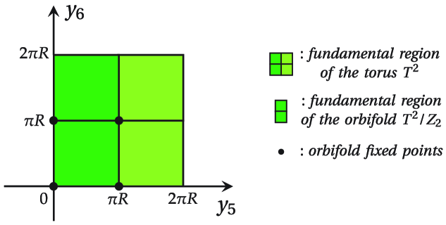
Figure 1: The fundamental region of the orbifold $T^{2}/Z_{2}$ and the four fixed points on it.

3.1 Scalar

We introduce a brane-localized mass at a fixed point corresponding to the origin of two extra directions, i.e., $z=z_{1}\,(=0)$. The Lagrangian for the complex 6D scalar field under consideration is given as

$${\cal L}=-|D_{M}\Phi(x^{\mu},z)|^{2}-h\,|\Phi(x^{\mu},z)|^{2}\delta^{2}({z-z_{1}}).$$ (30)

Here, the real dimensionless variable $h$ denotes the scalar mass localized at the fixed point, where the mass scale is provided by the radius $R$. Also, this Lagrangian straightforwardly provides the six-dimensional equation of motion,

$$D_{M}D^{M}\Phi-h\,\Phi\delta^{2}({z-z_{1}})=0.$$ (31)

By substituting the KK-expanded scalar (6) for Eq. (30), the effective Lagrangian after dimensional reduction is calculated as

$${\cal L}_{\rm eff} =-\sum_{n,j}(\partial_{\mu}\varphi_{n}^{j})^{\dagger}(\partial^{\mu}\varphi_{n}^{j})$$

$$\phantom{=\ }-\sum_{n,n^{\prime}}\sum_{j,j^{\prime}}(\varphi_{n}^{j})^{\dagger}\left(\int d^{2}z\,(D\phi^{j}_{T^{2}/Z_{2},n}(z))^{\dagger}\bigl{(}D\phi^{j^{\prime}}_{T^{2}/Z_{2},n^{\prime}}(z)\bigr{)}+h(\phi^{j}_{T^{2}/Z_{2},n}({z_{1}}))^{\dagger}\phi^{j^{\prime}}_{T^{2}/Z_{2},n^{\prime}}({z_{1}})\right)\varphi_{n^{\prime}}^{j^{\prime}}$$

$$\equiv{\cal L}_{\rm kin}-\sum_{n,n^{\prime}}\sum_{j,j^{\prime}}(\varphi_{n}^{j})^{\dagger}{\cal M}^{2}_{(n,j),(n^{\prime},j^{\prime})}\varphi_{n^{\prime}}^{j^{\prime}},$$ (32)

where $\mathcal{L}_{\text{kin}}$ represents the kinetic terms of KK scalar particles, which are canonically normalized. The explicit form of the KK mass matrix after the perturbation is given as

$${\cal M}^{2}_{(n,j),(n^{\prime},j^{\prime})} ={\frac{2\pi M}{\cal A}(2n+1)\delta_{n,n^{\prime}}\delta_{j,j^{\prime}}+h\,(\phi^{j}_{T^{2}/Z_{2},n}(z_{1}))^{\dagger}(\phi^{j^{\prime}}_{T^{2}/Z_{2},n^{\prime}}(z_{1}))}$$

$$={m_{0}^{2}}\,(2n+1)\delta_{n,n^{\prime}}\delta_{j,j^{\prime}}+2h\,(v_{n,j})^{\dagger}v_{n^{\prime},j^{\prime}}\quad$$ (33)

with $m_{0}^{2}=2\pi M/{\cal A}$, where we adopt the shorthand notation

$$v_{n,j} \equiv\frac{1}{\sqrt{2}}\phi^{j}_{T^{2}/Z_{2},n}({z_{1}})=\phi^{j}_{n}({z_{1}})$$

$$=\frac{{\cal N}_{j}}{\sqrt{{2^{n}n!}}}\sum_{\ell\in\mathbb{Z}}e^{-\pi M(\frac{j}{M}+\ell)^{2}}H_{n}\bigl{(}\sqrt{2\pi M}(\tfrac{j}{M}+\ell)\bigr{)}.$$ (34)

Here, we mention the sign of the parameter $h$. When $h$ is positive/negative, no/possible tachyonic modes appear in the spectrum.

An extension to the localized mass term at the other fixed points is straightforward; all we need to do is change $z_{1}$ to $z_{i}\,\,(i=2,3,4)$ in $v_{n,j}$. Here, we comment on the fourth fixed point $z_{4}$ and effects from the localized mass on it. Via direct calculations, we obtain

$$\phi^{j}_{T^{2}/Z_{2},n}(-z_{k})=(-1)^{M\delta_{k,4}}\,{\eta}\,\phi^{j}_{T^{2}/Z_{2},n}(z_{k})$$ (35)

for $k=1,2,3,4$. This implies that when $\eta=-1$ there is no effect, except for $k=4$ with odd $M$. In this paper, we restrict ourselves to the case of $\eta=+1$. Such brane-localized mass terms of the scalar field possibly affect physics at low energies. Hence, we are interested in the eigenvalues and eigenvectors of the perturbed mass matrix in Eq. (33). We note that the above relation is also derived from the pseudoperiodic boundary conditions on both $T^{2}$ and $T^{2}/Z_{2}$ (see, e.g., Ref. [15]),

$$\phi^{j}_{T^{2}\text{ or }T^{2}/Z_{2},n}(z+1)=e^{iq\chi_{1}(z)}\phi^{j}_{T^{2}\text{ or }T^{2}/Z_{2},n}(z),$$ (36)

$$\phi^{j}_{T^{2}\text{ or }T^{2}/Z_{2},n}(z+i)=e^{iq\chi_{i}(z)}\phi^{j}_{T^{2}\text{ or }T^{2}/Z_{2},n}(z),$$ (37)

$$\chi_{1}(z)=\frac{b}{2}\text{Im}(z),\quad\chi_{i}(z)=-\frac{b}{2}\text{Im}(iz),$$ (38)

by setting $z$ as $0$, $-1/2$, $-i/2$, or $-(1+i)/2$. We will diagonalize this KK mass matrix in the following.

First of all, we comment on the cutoff scale. Unfortunately, extra-dimensional models are nonrenormalizable, and hence they should be considered as a kind of LEET of a more fundamental theory, e.g., string theory at a scale below the cutoff scale $\Lambda$. In the following discussion, we define the cutoff scale as a certain level of the KK masses, i.e.,

$$m_{0}^{2}<m_{1}^{2}\,(=3m_{0}^{2})<...<{m^{2}_{n_{\text{max}}}}\equiv\Lambda^{2}<{m^{2}_{n_{\text{max}}+1}}<{\cdots},$$ (39)

where $\Lambda$ is related to the size of the perturbed KK mass matrix by turning on the brane-localized mass term.

Also, a few comments about the cutoff of theories in extra dimensions are in order. When the reference energy in the renormalization group evolution crosses the mass of KK particles, beta functions take contributions from the states. Cumulative spectra of KK particles, which are a generic structure of compact extra dimensions, lead to a rapid increase and decrease of effective 4D couplings immediately once the reference scale passes the lowest KK state (see, e.g., Ref. [27, 28, 29]). Therefore, in general the cutoff scale should be close to the typical size of KK particles. When the cutoff scale is not very far away from the electroweak scale, corrections via higher-dimensional operators are not suppressed. On the other hand, when the KK mass scale is far away from the electroweak scale, such contributions are subdued (though the cutoff scale is close to the typical scale of KK states). Hence, for an extra-dimensional theory with a sufficiently heavier KK mass scale compared with the scale of electroweak physics, the fact that the cutoff scale should be near the typical scale of KK particles does not seem to be problematic.

It is convenient to relabel the indices $(n^{(\prime)},j^{(\prime)})$ in the KK mass matrix in Eq. (33) in terms of a new label $\alpha$. We describe the degeneracy of the wave functions for even $n$ (odd $n$) by $d_{e}$ ($d_{o}$), which gives us the useful relation $M=d_{e}+d_{o}$. We can define a one-to-one labeling as shown in Table 4. For example, when $M=3$, an explicit correspondence between $\alpha$ and $(n,j)$ (up to the ninth mode) is shown in Table 4. In terms of this labeling, the KK mass matrix (“wavefunction vector”) is expressed as ${\cal M}^{2}_{(n,j),(n^{\prime},j^{\prime})}\to{\cal M}^{2}_{\alpha,\beta}$ ($v_{n,j}\to v_{\alpha}$), respectively. Also, by use of the information in Tables 2 and 2, the size of the mass matrix is easily estimated as

$${\alpha_{\text{max}}=\begin{cases}M\times(k-1)+d_{e}&\text{for }n_{\text{max}}=2(k-1),\\ M\times k&\text{for }n_{\text{max}}=2k-1,\end{cases}\qquad\left(k=1,2,3,\cdots\right),}$$ (40)

$\alpha$	$1$	$2$	…	$d_{e}$	$d_{e}+1$	$d_{e}+2$	…	$M$	$M+1$	$M+2$	…	$M+d_{e}$	…
$n$	$0$	$0$	…	$0$	$1$	$1$	…	$1$	$2$	$2$	…	$2$	…
$j$	$0$	$1$	…	$d_{e}-1$	$1$	$2$	…	$d_{o}$	$0$	$1$	…	$d_{e}-1$	…

Table 3: Relationships between $\alpha$ and $(n,j)$.

$\alpha$	$1$	$2$	$3$	$4$	$5$	$6$	$7$	$8$	$9$	…
$(n,j)$	$(0,0)$	$(0,1)$	$(1,1)$	$(2,0)$	$(2,1)$	$(3,1)$	$(4,0)$	$(4,1)$	$(5,1)$	…

Table 4: Relationships between $\alpha$ and $(n,j)$ for $M=3$.

Now, we are ready to analyze the perturbed KK mass matrix. As a first illustration, let us consider $M=3$ and $\Lambda=m_{1}$, where $d_{e}=2$, ${d_{o}}=1$, and $\alpha$ runs over $1,2,3$. The corresponding $3\times 3$ KK mass matrix is given as

$${\cal M}^{2}_{\alpha,\beta}=\begin{pmatrix}m_{0}^{2}+2h|v_{1}|^{2}&2hv_{1}^{\dagger}v_{2}&2hv_{1}^{\dagger}v_{3}\\ 2hv_{2}^{\dagger}v_{1}&m_{0}^{2}+2h|v_{2}|^{2}&2h{v_{2}^{\dagger}v_{3}}\\ 2hv_{3}^{\dagger}v_{1}&2hv_{3}^{\dagger}v_{2}&m_{1}^{2}+2h|v_{3}|^{2}\end{pmatrix},$$ (41)

and three eigenvalues can be analytically solved as

$$m_{0}^{2},\quad 2m_{0}^{2}+h(|v_{1}|^{2}+|v_{2}|^{2}+|v_{3}|^{2})\pm\sqrt{(m_{0}^{2}+h(|v_{1}|^{2}+|v_{2}|^{2}+|v_{3}|^{2}))^{2}-4hm_{0}^{2}(|v_{1}|^{2}+|v_{2}|^{2})},$$ (42)

where we used the relation $m_{1}^{2}=3m_{0}^{2}$. Here, the eigenvalue is unperturbed as $m_{0}^{2}$. By focusing the property $|v_{\alpha}R|^{2}\lesssim 1$, which is recognized by the correct normalization of the mode functions, the other eigenvalues are roughly estimated as $m_{0}^{2}(1+{\cal O}(h))$ and $m_{1}^{2}(1+{\cal O}(h))$. Thus, we find that one of the original lowest KK masses, i.e., $m_{0}^{2}$ appears after turning on the brane-localized mass.

When the cutoff scale is chosen as $\Lambda=m_{3}$, where $\alpha=1,2,...,6$, the corresponding eigenvalues are calculated in a similar manner as $m_{0}^{2}$, $m_{0}^{2}(1+{\cal O}(h))$, $m_{1}^{2}(1+{\cal O}(h))$, $m_{2}^{2}$, $m_{2}^{2}(1+{\cal O}(h))$, and $m_{3}^{2}(1+{\cal O}(h))$. We find that one of the second excited states is also unperturbed.

The above discussion can be extended to the generic magnitude of the magnetic flux and an arbitrary cutoff scale. The KK mass matrix with a brane-localized mass can be symbolically expressed as

$${\cal M}^{2}={{\rm diag}\,(\underbrace{m_{0}^{2},m_{0}^{2},...,m_{0}^{2}}_{d_{e}},\,\underbrace{m_{1}^{2},m_{1}^{2},...,m_{1}^{2}}_{d_{o}},\,\underbrace{m_{2}^{2},m_{2}^{2},...,m_{2}^{2}}_{d_{e}},\,\cdots)}+v^{\dagger}\otimes v,$$ (43)

where ${(v)_{\alpha}}=(v_{1},v_{2},...)$ denotes an $\alpha_{\text{max}}$ component complex vector. For $d_{e}\geq 2$, there always exists an eigenvector for the lowest mode ($n=0$),

$$(u_{{n=0}})_{\alpha}=(u_{1},u_{2},...,u_{d_{e}},0,0,\cdots),$$ (44)

which satisfies $v\cdot u_{{n=0}}=0$. In the above example ($M=3$), there exist $d_{e}-1$ linearly independent eigenvectors that satisfy $v\cdot u_{{n=0}}=0$ as

$$\left(u^{{(1)}}_{{n=0}}\right)_{\alpha} =(\underbrace{-v_{2},v_{1},0,0,...,0}_{d_{e}},\,0,0,\cdots),$$ (45)

$$\left(u^{{(2)}}_{{n=0}}\right)_{\alpha} =(\underbrace{0,-v_{3},v_{2},0,...,0}_{d_{e}},\,0,0,\cdots),$$ (46)

$$\vdots$$

$$\left(u^{{(d_{e}-1)}}_{{n=0}}\right)_{\alpha} =(\underbrace{0,0,...,0,-v_{d_{e}},v_{d_{e}-1}}_{d_{e}},\,0,0,\cdots),$$ (47)

where we cannot take another eigenvector that is linearly independent of all of $u^{(1)}_{{n=0}}$, $u^{(2)}_{{n=0}}$, …, $u^{(d_{e}-1)}_{{n=0}}$. This fact suggests that one of the lowest modes is uplifted by the perturbation after turning on the brane-localized mass. For any level of the degenerate mass eigenvalues before the perturbation, we find that such vectors provide the corresponding eigenvalue as

$${{\cal M}^{2}u_{n}=m_{n}^{2}u_{n}+v^{\dagger}(v\cdot u_{n})=m^{2}_{n}u_{n}}.$$ (48)

We would like to comment on the effects from multiple localized mass terms. For example, we turn on two localized masses $h_{1}|\Phi|^{2}$ and $h_{2}|\Phi|^{2}$ at $z=z_{1}$ and $z=z_{2}$, respectively. Here, the corresponding KK mass matrix is

$$\left({\cal M}^{2}\right)_{\alpha,\beta}=(2n+1)m_{0}^{2}\delta_{\alpha,\beta}+2h_{1}v^{(1){\dagger}}_{\alpha}v^{(1)}_{\beta}+2h_{2}v^{(2){\dagger}}_{\alpha}v^{(2)}_{\beta},$$ (49)

where we define

$$v^{(1)}_{\alpha} \equiv v^{(1)}_{n,j}=\phi^{j}_{n}(z_{1}),$$ (50)

$$v^{(2)}_{\alpha} \equiv v^{(2)}_{n,j}=\phi^{j}_{n}(z_{2}).$$ (51)

The degeneracies of the KK states via magnetic fluxes are degraded one by one as we place the brane-localized mass. We provide a detailed discussion on such cases in Appendix B.

Before closing this section, it is important to mention a 6D vector field, which is decomposed into a (4D) vector component ($A_{\mu}$) and two scalar components ($A_{5,\,6}$) from the four-dimensional point of view. The KK mass spectra of a vector field which feels magnetic fluxes on a flux background were analyzed in Ref. [25], which provided KK eigenvalues of the two corresponding 4D scalars of $\phi_{n,z}\equiv(A_{5}+iA_{6})/\sqrt{2}$ as

$$m_{n}^{2}=\frac{2\pi M}{\cal A}(2n-1),$$ (52)

and of $\phi_{n,\bar{z}}\equiv(A_{5}-iA_{6})/\sqrt{2}$ as

$$m_{n}^{2}=\frac{2\pi M}{\cal A}(2(n+1)+1),$$ (53)

where the spectrum of the vector field is equivalent to $\phi_{n,\bar{z}}$ through suitable gauge fixing. Here, we would pay attention to two points. One is that the equation of motion of the 6D scalar $\Phi$ takes a different form than those of $\phi_{n,z}$ and $\phi_{n,\bar{z}}$, which leads to the difference in the mass spectra. The other is that in the present Abelian case, the 6D vector field does not feel any magnetic flux. The situation where the 6D vector field couples to magnetic flux is realized in a non-Abelian gauge theory, which is a reasonable playground for unified theories.

From Eq. (52), we recognize a pathology of the emergence of the tachyonic state in $\phi_{n=0,z}$, which is a critical obstacle for constructing reasonable models. An ordinary remedy for conquering the difficulty is to address supersymmetrized theories, where if 4D $\mathcal{N}=1$ supersymmetry remains in the action (before taking into account the connection to the supersymmetry-breaking sector), such tachyonic states are stabilized (see, e.g., Refs. [23, 25]). On the other hand, issues discussed in this manuscript would provide another clue to circumventing the obstacle by uplifting the tachyonic mode via a brane-localized mass term for $\phi_{n,z}$.

When localized mass terms, e.g., $hA_{5}^{2}$ (and $hA_{6}^{2}$) are induced after non-Abelian gauge symmetry breaking (i.e., introducing fluxes and/or Wilson lines) the above discussion is relevant for analyzing the KK mass matrix of such kinds of scalars, in spite of the difference in the pattern of the KK masses.

3.2 Spinor

We express the 6D Weyl spinor as $\Psi=(\lambda_{+},\lambda_{-})^{\text{T}}$ in terms of four-component Weyl spinors $\lambda_{+}$ and $\lambda_{-}$. Then, its KK decomposition is given as

$$\lambda_{+}(x^{\mu},z)={\sum_{n,j}\chi_{+,n}^{j}(x^{\mu})\otimes\psi_{T^{2}/Z_{2}\,+,n}^{j}(z)},$$ (54)

$$\lambda_{-}(x^{\mu},z)={\sum_{n,j}\chi_{-,n}^{j}(x^{\mu})\otimes\psi_{T^{2}/Z_{2}\,-,n}^{j}(z)}.$$ (55)

The Lagrangian for the 6D Weyl spinor is given as

$${\cal L}=i\bar{\Psi}\Gamma^{M}D_{M}\Psi+(i\bar{\nu}\gamma^{\mu}\partial_{\mu}\nu-g(\bar{\nu}\lambda_{+}+{\rm{H}.c.}))\delta^{2}(z-z_{k}),$$ (56)

where $g$ is a massless parameter associated with the localized mass of the spinor. Note that the 6D Weyl spinor cannot possess a Dirac mass term such as $\bar{\Psi}\Psi$ [7]. Then, we add a four-dimensionally localized Weyl spinor field $\nu(x^{\mu})$ and introduce a localized mass term at a fixed point $z_{k}$.

In the following, we place the localized mass at a fixed point of $T^{2}/Z_{2}$ [see Eq. (29)]. It is easily found that $\lambda_{-}(x^{\mu},{z_{k}})=0$ ($\lambda_{+}(x^{\mu},{z_{k}})=0$) [${k}=1,2,3$] for $\eta=+1$ ($\eta=-1$), respectively. Hence, we cannot introduce such a mass for $\lambda_{-}$ at the three fixed points. Therefore, we focus on the case of $\eta=+1$, as in the previous section. It is straightforward to expect that we can similarly analyze the case of $\eta=-1$. Hereafter, we choose the 6D chirality of $\Psi$ as $-1$, which means that left-handed chiral modes are realized as zero modes of $\lambda_{+}$ (see Appendix A). The 4D chirality of $\nu$ is automatically determined to be right-handed.

The spinor Lagrangian in Eq. (56) provides the six-dimensional equations of motion,

$$i\gamma^{\mu}\partial_{\mu}\lambda_{+}+D^{\dagger}\lambda_{-}-g\nu\delta^{2}({z-z_{k}}) =0,$$ (57)

$$i\gamma^{\mu}\partial_{\mu}\lambda_{-}-D\lambda_{+} =0,$$ (58)

$${\left(i\gamma^{\mu}\partial_{\mu}\nu-g{\lambda_{+}}\right)}\delta^{2}(z-z_{k}) =0.$$ (59)

Removing $\lambda_{-}$ and $\nu$ from these equations leads to the (six-dimensional) equation of motion for $\lambda_{+}$,

$${\left(\partial_{\mu}\partial^{\mu}+D^{\dagger}D\right)}\lambda_{+}-{g^{2}}\lambda_{+}\delta^{2}({z-z_{k}})=0,$$ (60)

where the operator $D^{\dagger}D$ is equal to $\Delta-2\pi M/\mathcal{A}$, which indicates the mass difference in the fermion case and scalar case as shown in Eqs. (13) and (15) when $g=0$.

By plugging the KK decompositions (54) and (55) into Eq. (56), the effective Lagrangian under the cutoff scale is calculated as

$${\cal L}_{\rm eff} ={\cal L}_{\rm kin}-\sum_{{n,j\atop(n\not=0)}}\left(m_{n}{\bar{\chi}}^{j}_{+,n}{}_{L}\chi^{j}_{-,n}{}_{R}+g{\bar{\nu}}_{R}\chi_{+,0}^{j}{}_{L}\psi^{j}_{T^{2}/Z_{2}\,+,0}({z_{k}})+g{\bar{\nu}}_{R}\chi^{j}_{+,n}{}_{L}\psi^{j}_{T^{2}/Z_{2}\,+,n}({z_{k}})+{\rm{H}.c.}\right)$$

$$\equiv{\cal L}_{\rm kin}-\sum_{{n,j\atop(n\not=0)}}(\bar{\nu}_{R},\,{\bar{\chi}}_{-,n}^{j}{}_{R}){\cal M}\begin{pmatrix}{\chi}^{j}_{+,0}{}_{L}\\[3.0pt] {\chi}^{j}_{+,n}{}_{L}\end{pmatrix}+{\rm{H}.c.},$$ (61)

where $\mathcal{L}_{\text{kin}}$ contains kinetic terms and the corresponding 4D chiralities are explicitly shown for clarity. The perturbed KK mass matrix $\mathcal{M}$ under the brane-localized spinor mass term is symbolically expressed as

$${\cal M}=\begin{pmatrix}\sqrt{2}\,{g}\psi^{j}_{+,0}({z_{k}})&\sqrt{2}\,{g}\psi^{j}_{+,n}({z_{k}})\\[3.0pt] 0&m_{n}\end{pmatrix}.$$ (62)

Here, note that the index $n$ takes nonzero positive integer values in the above expressions, and also that we use the relation $\psi^{j}_{T^{2}/Z_{2}\,+,n}({z_{k}})=\sqrt{2}\psi^{j}_{+,0}({z_{k}})$. Here, the size of $\mathcal{M}$ is $(1+N_{\text{KK}})\times(d_{e}+N_{\text{KK}})$, where $N_{\text{KK}}$ represents the number of excited KK modes that appear up to the level designated by $n_{\text{max}}$. The relation is easily understood among $N_{\text{KK}}$ and $\alpha_{\text{max}}$ as defined in Eq. (40),

$${N_{\text{KK}}=\alpha_{\text{max}}-d_{e},}$$ (63)

because $d_{e}$ represents the number of zero modes.

Since the matrix $\mathcal{M}$ is asymmetric, it is convenient to consider the following two forms of products of the matrix

$$({\cal MM}^{\dagger})_{\alpha,\beta} ={(\Pi^{2}_{R})_{\alpha,\beta}+\sqrt{2}\,{g}(V^{\dagger}_{R}\Pi_{R})_{\alpha}\,\delta_{0,\beta}+\sqrt{2}\,{g}(\Pi_{R}V_{R})_{\beta}\,\delta_{0,\alpha}}$$

$$\quad{+2{g^{2}}\left[\sum_{j=0}^{d_{e}-1}|v_{0,j}|^{2}+\sum_{\rho=1}^{N_{\text{KK}}}|(V_{R})_{\rho}|^{2}\right]{\delta_{0,\alpha}\delta_{0,\beta}}\qquad(\alpha,\beta=0,1,\cdots,N_{\text{KK}})},$$ (64)

$$({\cal M}^{\dagger}{\cal M})_{\alpha,\beta} ={(\Pi^{2}_{L})_{\alpha,\beta}+\sqrt{2}\,{g}(V^{\dagger}_{R})_{\alpha}(V_{R})_{\beta}\qquad(\alpha,\beta=1,2,\cdots,\alpha_{\text{max}}{=N_{\text{KK}}+d_{e}})},$$ (65)

for the right- and left-handed Weyl spinors $(\nu_{R},{\chi}_{-,n}^{j}{}_{R})$ and $({\chi}^{j}_{+,0}{}_{L},{\chi}^{j}_{+,n}{}_{L})$, respectively. Here, we see that $\alpha=0$ corresponds to the 4D localized field $\nu_{R}$ in Eq. (64). The sizes of the matrices ${\cal MM}^{\dagger}$ and ${\cal M}^{\dagger}{\cal M}$ are $(1+N_{\text{KK}})\times(1+N_{\text{KK}})$ and $(d_{e}+N_{\text{KK}})\times(d_{e}+N_{\text{KK}})$, respectively. Also, we define the following symbols

$$(\Pi_{R})_{\alpha,\beta} \equiv{\rm diag}(0,\,\underbrace{m_{1},m_{1},...,m_{1}}_{d_{o}},\,\underbrace{m_{2},m_{2},...,m_{2}}_{d_{e}},\cdots),$$ (66)

$$(V_{R})_{\alpha} \equiv(0,\,\underbrace{v_{1,1},v_{1,2},...,v_{1,d_{o}}}_{d_{o}},\,\underbrace{v_{2,0},v_{2,1},...,v_{2,d_{e}-1}}_{d_{e}},\,\cdots)^{\text{T}},$$ (67)

$$(\Pi_{L})_{\alpha,\beta} \equiv{\rm diag}(\underbrace{0,0,...,0}_{d_{e}},\,\underbrace{m_{1},m_{1},...,m_{1}}_{d_{o}},\,\underbrace{m_{2},m_{2},...,m_{2}}_{d_{e}},\cdots),$$ (68)

$$(V_{L})_{\alpha} \equiv(\underbrace{v_{0,0},v_{0,1},...,v_{0,d_{e}-1}}_{d_{e}},\,\underbrace{v_{1,1},v_{1,2},...,v_{1,d_{o}}}_{d_{o}},\,\underbrace{v_{2,0},v_{2,1},...,v_{2,d_{e}-1}}_{d_{e}},\,\cdots)^{\text{T}},$$ (69)

with $v_{n,j}\equiv\psi^{j}_{+,n}({z_{k}})$.

In the spinor case, we recognize that the mass spectrum of the left-handed modes $\chi_{+,0}^{j}{}_{L}$ and $\chi_{+,n}^{j}{}_{L}$ is equivalent to that of the scalar because the mass matrix squared in Eq. (65) takes the same form as that in the scalar case.

On the other hand, we analyze the mass spectra of the 4D brane-localized field $\nu_{R}$ and the right-handed modes ${\chi}_{-,n}^{j}{}_{R}$. For a vector $(u)_{\alpha}\,\,(\alpha=0,1,\cdots,N_{\text{KK}})$, we calculate the product of $({\cal MM}^{\dagger})_{\alpha,\beta}$ and $u_{\alpha}$ as

$$\sum_{\beta=0}^{N_{\text{KK}}}({\cal MM}^{\dagger})_{\alpha,\beta}(u)_{\beta}=\begin{cases}\displaystyle\sqrt{2}\,{g}\sum_{\beta=1}^{N_{\text{KK}}}(\Pi_{R}V_{R})_{\beta}(u)_{\beta}+2{g^{2}}\left[\sum_{j=0}^{d_{e}-1}|v_{0,j}|^{2}+\sum_{{\rho}=1}^{N_{\text{KK}}}|(V_{R})_{\rho}|^{2}\right](u)_{0}&(\alpha=0),\\[5.0pt] \displaystyle\sum_{\beta=0}^{N_{\text{KK}}}(\Pi^{2}_{R})_{\alpha,\beta}(u)_{\beta}+\sqrt{2}\,{g}(V^{\dagger}_{R}\Pi_{R})_{\alpha}(u)_{0}&(\alpha\geq 1).\end{cases}$$ (70)

Equation (70) implies that $\nu_{R}$ is perturbed by the presence of the localized mass since the right-hand side for $\alpha=0$ may be nonvanishing in almost all cases. This is understood as follows. Since the right-handed spinors $\chi^{j}_{-,n}{}_{R}$ are originally massive around the compactification scale ($\sim 1/\sqrt{\cal A}$), we can determine whether $\nu_{R}$ is massless or massive only by investigating the determinant of ${\cal MM}^{\dagger}$. This is because the determinant of a matrix is equal to the product of its eigenvalues. If the determinant is nonzero, we can conclude that $\nu_{R}$ becomes massive.

Here, let us focus on a simple example for $M=3$ and $\Lambda=m_{2}$. For the right-handed fields $(\nu_{R},{\chi}_{-,1}^{0}{}_{R},{\chi}_{-,1}^{1}{}_{R},{\chi}_{-,2}^{1}{}_{R})$, the $4\times 4$ KK mass matrix squared ${\cal MM}^{\dagger}$ is symbolically written with the symbols $a$, $b$, $c$ and $d$ as

$${\cal MM}^{\dagger}=\begin{pmatrix}{2}\,{g^{2}}d&{\sqrt{2}}\,{g}a\,{m_{1}}&{\sqrt{2}}\,{g}b\,{m_{1}}&{\sqrt{2}}\,{g}c\,{m_{2}}\\ {\sqrt{2}}\,{g}a^{\dagger}{m_{1}}&{m_{1}^{2}}&0&0\\ {\sqrt{2}}\,{g}b^{\dagger}{m_{1}}&0&{m_{1}^{2}}&0\\ {\sqrt{2}}\,{g}c^{\dagger}{m_{2}}&0&0&{m_{2}^{2}}\end{pmatrix}.$$ (71)

Here, $g$ is a dimensionless coefficient in the localized mass term of the spinor field. The determinant of this matrix is calculated as

$${\det\left({\cal MM}^{\dagger}\right)=2{g^{2}}m_{1}^{4}m_{2}^{2}\left(d-|a|^{2}-|b|^{2}-|c|^{2}\right),}$$ (72)

where mass dimensions of the four symbols are two (for $d$) and one (for $a,b,c$). For a nonzero coefficient ($g\neq 0$), a miraculous cancellation should occur among the symbols $a,b,c$ and $d$ to realize $\det{\cal MM}^{\dagger}=0$, which suggests that $\nu_{R}$ is still massless after the localized-mass perturbation. Although we note that we could not find a concrete example where the cancellation happens, our conclusion is that $\nu_{R}$ gets a mass via the localized mass in almost any case. When $M$ and/or $\Lambda$ is arbitrary, configurations of nonzero components in the mass matrix squared $\mathcal{M}\mathcal{M}^{\dagger}$ look similar. Therefore, this kind of discussion is still valid.

The matrices ${\cal MM}^{\dagger}$ and $\mathcal{M}^{\dagger}\mathcal{M}$ contain $N_{\text{KK}}+1$ and $N_{\text{KK}}+d_{e}$ numbers of squared mass eigenvalues, respectively, where $N_{\text{KK}}$ values are common in both of the matrices. These modes mainly originate from the KK mass terms $\overline{\chi}^{j}_{-,nR}\chi^{j}_{+,nL}+\text{H.c.}$ which exist even before the perturbation.

4 Deformations of the KK wave functions

As discussed in Sec. 3, we found that at least one of the lowest KK masses remains after introducing one brane-localized mass term if the number of the lowest modes is greater than or equal to two. In this section, we investigate what happens on the corresponding KK wave function after the perturbation.

A physical sense of such deformations is a possible modulation of three-point effective interactions, i.e., Yukawa couplings in phenomenological models, which are characterized by the overlap integrals of three types of KK wavefunctions. The Yukawa couplings on $T^{2}/Z_{2}$ are expressed as

$$y_{{\alpha\beta\gamma}}\sim\int_{{T^{2}}}d^{2}z\,\psi_{T^{2}/Z_{2}}^{{\alpha}}(z)\psi_{T^{2}/Z_{2}}^{{\beta}}(z)(\phi_{T^{2}/Z_{2}}^{{\gamma}}(z))^{\dagger},$$ (73)

where $\alpha$, $\beta$ and $\gamma$ discriminate the physical eigenstates on magnetized $T^{2}/Z_{2}$ before the perturbation by turning on single or multiple brane-localized mass terms. For example, when we introduce a localized mass term for the 6D scalar field, the profiles of KK mode functions describing the lowest states would be changed as $\phi_{T^{2}/Z_{2}}^{\alpha}(z)\,\,({\alpha}={1,2,...,{d_{e}}})\to\phi^{{i_{\text{mass}}}}_{{T^{2}/Z_{2}}}(z)\,\,({i_{\text{mass}}}={1,2,...,{d_{e}}-1})$. Accordingly, the Yukawa couplings are expected to be changed as

$$\int_{{T^{2}}}d^{2}z\,\psi_{T^{2}/Z_{2}}^{{\alpha}}(z)\psi_{T^{2}/Z_{2}}^{{\beta}}(z)(\phi_{T^{2}/Z_{2}}^{{\gamma}}(z))^{\dagger}\to\int_{{T^{2}}}d^{2}z\,\psi_{T^{2}/Z_{2}}^{{\alpha}}(z)\psi_{T^{2}/Z_{2}}^{{\beta}}(z)(\phi_{{T^{2}/Z_{2}}}^{{i_{\text{mass}}}}(z))^{\dagger}.$$ (74)

It is also expected that the same holds for localized mass terms of the spinor. Although we do not analyze such Yukawa couplings in the presence of brane-localized masses in this paper, it is important to investigate the change of the lowest KK mode functions.

As an illustrative example, we consider a simple example in the scalar case for $M=3$ and $\Lambda=m_{1}=18\pi/{\cal A}$, and then $\alpha=1,2,3$ [corresponding to $(n,j)=(0,0),(0,1),(1,1)$]. Then, the KK mass matrix under consideration is the same as the expression in Eq. (41). For $h=0.5$, the eigenvalues (divided by $m_{0}$) of Eq. (41) are numerically obtained as

$${(m/m_{0})^{2}=1.00000,\ 1.08008,\ 3.05828},$$ (75)

and also the corresponding eigenvectors are given as

$${u^{(1)}}=(0.459701,-0.888074,0),\ {u^{(2)}=(-0.88755,-0.45943,0.0343449)},$$

$${u^{(3)}=(0.0305008,0.0157884,0.99941)}.$$ (76)

The corresponding wave functions unaffected/affected by the brane-localized mass are obtained by internal products of the above eigenvectors and the KK wave functions before the perturbation $\phi_{\alpha}\equiv(\phi^{0}_{T^{2}/Z_{2},0},\phi^{1}_{T^{2}/Z_{2},0},\phi^{1}_{T^{2}/Z_{2},1})$, i.e.,

$$\phi^{i_{\rm mass}}(z)\equiv\sum_{\alpha=1}^{3}\left(u^{(i_{\rm mass})}\right)_{\alpha}\phi_{\alpha}(z)\qquad\left(i_{\text{mass}}=1,\,2,\,3\right).$$ (77)

We show the probability densities $|\phi^{i_{\rm mass}}(z)|^{2}$ of the KK wave functions with mass eigenvalues that are unaffected/perturbed by the brane-localized mass at $z=z_{1}$ for $M=3$ in Fig. 2, where a red cross denotes a position with the brane-localized mass. Figure 2 tells that an unaffected mode ($i_{\rm mass}=1$) avoids the position with the localized mass, and also that the other affected modes ($i_{\rm mass}=2,3$) are localized at the position with the localized mass. The trend that unaffected modes avoid the position with the localized mass is also found in situations with multiple localized masses (see Fig. 3).

We provide another example with $M=4$ and $\Lambda=m_{1}$ ($\alpha=1,2,3,4$), and two brane-localized mass terms at the two fixed points $z=z_{1}$ and $z=z_{2}$. The sketches of wave function localizations are shown in Fig. 3. Here, we can see that two of the three lowest modes before the perturbation (see Table 2) are uplifted.

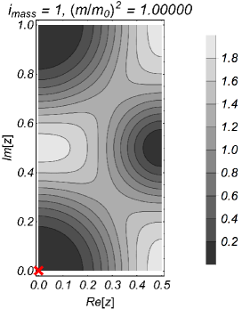
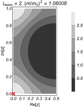
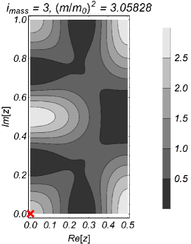
Figure 2: The probability densities $|\phi^{i_{\rm mass}}(z)|^{2}$ of the KK wave functions with mass eigenvalues that are unaffected ($i_{\text{mass}}=1$)/perturbed ($i_{\text{mass}}=2,\,3$) by the brane-localized mass at $z=z_{1}$ for $M=3$ and $h=0.5$. A red cross denotes a position with the brane-localized mass. The corresponding mass eigenvalues after the perturbation are also shown. The values of the ratio $(m/m_{0})^{2}$ before the perturbation are $1$, $1$, and $3$, respectively.

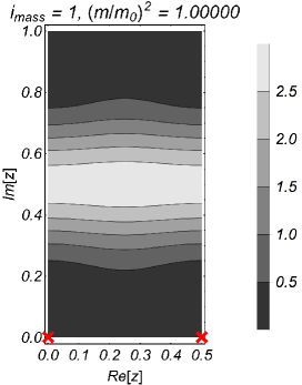
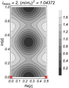
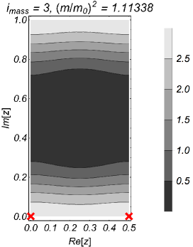
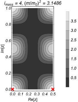
Figure 3: The probability densities $|\phi^{i_{\rm mass}}(z)|^{2}$ of the KK wave functions with mass eigenvalues that are unaffected ($i_{\text{mass}}=1$)/perturbed ($i_{\text{mass}}=2,\,3,\,4$) by the brane-localized mass terms at $z=z_{1}$ and $z=z_{2}$ for $M=4$ and $h=0.5$. The two red crosses in each panel denote the positions where the brane-localized mass terms are located. The corresponding mass eigenvalues after the perturbation are also shown. The values of the ratio $(m/m_{0})^{2}$ before the perturbation are $1$, $1$, $1$, and $3$, respectively.

5 Cutoff dependence of mass eigenvalues

Once we specify a cutoff scale $\Lambda$, we can write down the KK mass spectra with the brane-localized mass below $\Lambda$. As concretely addressed in the previous section, when $\eta=+1$ and $M\geq 2$, a part of the lowest modes of the KK mass spectrum in the scalar is unaffected by the presence of a single localized mass term, where the values of such unperturbed mass eigenstates are independent of the cutoff scale $\Lambda$. On the other hand, some mass eigenvalues are perturbed and get heavier by the effect of the localized mass term, where the degree of such deformations would depend on the cutoff scale. We suppose that $\Lambda=m_{n_{\rm max}}$ for a certain $n_{\rm max}$. Hereafter, we consider $n_{\rm max}$ instead of $\Lambda$.

As before, we focus on $M=3$. The two lowest modes without localized masses are doubly degenerate and their KK masses are ${m_{0}^{2}}=6\pi/{\cal A}$. After introducing a localized mass at $z=z_{1}$, one of the two lowest modes gets heavier and the perturbed mass is roughly estimated as ${m^{2}\sim m_{0}^{2}}(1+{\cal O}(h))$, assuming that $|v_{\alpha}R|^{2}\sim{{\cal O}(1)}$. For the maximum of the KK levels $n_{\rm max}$, the ratio $(m/m_{0})^{2}$ can be interpolated as

$${\left(\frac{m}{m_{0}}\right)^{2}}\simeq\alpha_{1}+\alpha_{2}\ln n_{\rm max}+\alpha_{3}\,n_{\rm max},$$ (78)

where $\alpha_{i}\,\,(i=1,2,3)$ are real constants. The cutoff scale dependence of the (squared) mass ratio $(m/m_{0})^{2}$ is shown in Fig. 4 (Fig. 5), where we set $h=0.5$ ($h=3.0$), respectively. Figures 4 and 5 tell us that the choic of cutoff scale does not drastically affect the mass ratio, and we can conclude that such a cutoff dependence is irrelevant from a model-building point of view [except for $h$ being as huge as $\gtrsim\mathcal{O}(10)$ and/or the compactification scale $\sim R^{-1}$ being as small as $\lesssim{\mathcal{O}(1)}\,\text{TeV}$]. We also find that the cutoff dependence looks similar and would be irrelevant for greater magnitudes of the fluxes. Also, we would like to comment on the testability of the mass correction via localized masses through high-energy experiments. When the coefficient of a localized mass $h$ is small, the cutoff dependence is negligible (as already explained) and it seems difficult to probe the effect by discovering several KK modes and measuring the mass differences among them. Thus, the mechanism has difficulties from the testability point of view. However, the main motivation of this research is to reveal the relationship between the presence of localized masses and the number of fluxes (corresponding to the number of unperturbed matter generations).

When we consider a high-scale extra-dimensional theory, the correction in KK states (before the mass perturbation) seems to be less important. Nevertheless, we can claim that the stability of the values of heavier states (compared with the electroweak scale) against the perturbation is a good feature of the present scenario.

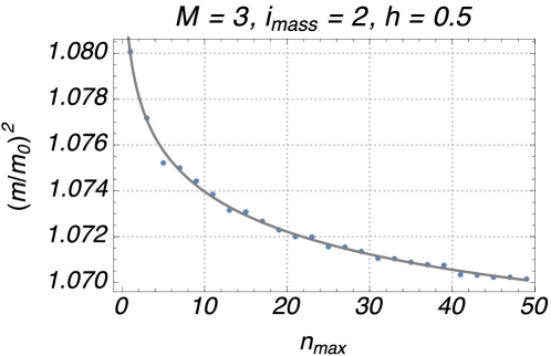
Figure 4: The cutoff scale dependence of the squared mass ratio $(m/m_{0})^{2}$ for a perturbed mode. Fitting parameters are chosen as $(\alpha_{1},\alpha_{2},\alpha_{3})={(1.07999,-0.00265445,9.10443\times 10^{-6})}$. Note that the ratio before the perturbation is $(m/m_{0})^{2}=1.$

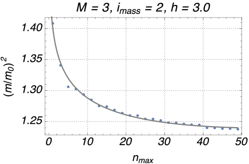
Figure 5: The cutoff scale dependence of the squared mass ratio $(m/m_{0})^{2}$ for a perturbed mode. Fitting parameters are chosen as $(\alpha_{1},\alpha_{2},\alpha_{3})={(1.39949,-0.0523681,0.0009029)}$. Note that the ratio before the perturbation is $(m/m_{0})^{2}=1.$

6 Conclusion

In this paper, we have considered effects on the KK mass spectra via the presence of brane-localized masses at fixed points of a toroidal orbifold $T^{2}/Z_{2}$ with magnetic fluxes. Under the presence of the magnetic fluxes on the toroidal and orbifold compactifications, the magnetic fluxes are quantized and become topological indices, and then the multiplicity of KK-decomposing wave functions appears in the low-energy effective theory.

We have added single or multiple brane-localized masses at the fixed points of $T^{2}/Z_{2}$ where some parts of the KK spectrum on $T^{2}$ are projected out by the orbifolding, while multiple degenerated modes still remain (if $M\geq 2$). By analyzing the effects of the localized masses using linear algebra, we have found that, at each KK level, one or more of the degenerate KK masses are perturbed, when single or multiple brane-localized mass terms are introduced. This discussion is valid for both of the six-dimensional scalar and spinor fields. In addition, we have also investigated deformation in wave functions through the localized mass terms and the cutoff dependence of the magnitude of modulations in the mass eigenvalues.

The mechanism which we have investigated in this paper is useful for phenomenologies on magnetized orbifolds, especially in constructing unified theories with a much heavier KK scale compared with the electroweak scale, for decoupling some light exotic particles away from the physics around the electroweak and TeV scales. An important point in the mechanism in 6D is that particle spectra do not seriously depend on the magnitude of the coefficients of brane-localized mass terms when the KK scale is sufficiently higher than the electroweak scale, while the number of fixed points where brane-localized mass terms are injected plays a significant role. Therefore, we can conclude that our mechanism is useful for removing unwanted exotic light modes from low-energy effective theories without relying on the details of theories in extra dimensions.

Applications to more generalized situations with nontrivial Scherk-Schwarz and Wilson line phases as well as general choices in the complex structure parameter $\tau$ look fruitful.

Appendix A Notation

In this appendix, we review our notation for 6D gamma matrices, which obey the Clifford algebra

$$\{\Gamma^{M},\Gamma^{N}\}=-2g^{MN},\qquad g^{MN}=\text{diag}(-1,+1,+1,+1,+1,+1).$$ (79)

Our choice for the set of 6D gamma matrices is as follows:

$$\Gamma^{\mu}=\begin{pmatrix}\gamma^{\mu}&0\\ 0&\gamma^{\mu}\end{pmatrix},\qquad\Gamma^{5}=\begin{pmatrix}0&i\gamma_{5}\\ i\gamma_{5}&0\end{pmatrix},\qquad\Gamma^{6}=\begin{pmatrix}0&\gamma_{5}\\ -\gamma_{5}&0\end{pmatrix},$$ (80)

where $\gamma_{5}$ describes the 4D chirality, which is defined as $\gamma_{5}=i\gamma^{0}\gamma^{1}\gamma^{2}\gamma^{3}$. The matrix denotes the 6D chirality and can be decomposed as

$$\Gamma^{7}=-\Gamma^{0}\Gamma^{1}\Gamma^{2}\Gamma^{3}\Gamma^{5}\Gamma^{6}=\begin{pmatrix}\gamma_{5}&0\\ 0&-\gamma_{5}\end{pmatrix}=\Gamma_{\text{4D chiral}}\,\Gamma_{\text{internal}}$$ (81)

with

$$\Gamma_{\text{4D chiral}}=\begin{pmatrix}\gamma_{5}&0\\ 0&\gamma_{5}\end{pmatrix},\qquad\Gamma_{\text{internal}}\equiv i\Gamma^{5}\Gamma^{6}=\begin{pmatrix}I_{4}&0\\ 0&-I_{4}\end{pmatrix}.$$ (82)

The matrix $\Gamma_{\text{internal}}$ describes eigenvalues of the internal chirality. The 6D chirality is calculated as the simple product of the 4D chirality and the internal chirality.

Appendix B Generic discussion in the scalar case

In the main sections, we mainly discussed the effects arising from the presence of a single brane-localized mass. In this appendix, we extend the discussion to multiple brane-localized mass terms and their effects on KK mass eigenvalues. The scalar case is addressed in the following discussion, where the method to treat the fermion case is straightforwardly recognized through the result for the scalar. The reason is that $\mathcal{M}^{2}$ for the scalar and $\mathcal{M}^{\dagger}\mathcal{M}$ for the fermion take the same form, as we pointed out in Sec. 3.2.

For example, we add another brane-localized mass to Eq. (43), and then obtain

$${\cal M}^{2}={\rm diag}\,(\underbrace{m_{0}^{2},m_{0}^{2},...,m_{0}^{2}}_{d_{e}},\,\underbrace{m_{1}^{2},m_{1}^{2},...,m_{1}^{2}}_{d_{o}},\,\underbrace{m_{2}^{2},m_{2}^{2},...,m_{2}^{2}}_{d_{e}},\cdots)+(v^{(1)})^{{\dagger}}\otimes v^{(1)}+(v^{(2)})^{{\dagger}}\otimes v^{(2)}.$$ (83)

Here, we do not specify two distinct positions with the localized masses and symbolically express $(v^{(1)})_{\alpha}=\phi_{\alpha}(z_{i})$ and $(v^{(2)})_{\alpha}=\phi_{\alpha}(z_{j})$ for $z_{i}\neq z_{j}$. In order to keep one of the original lowest eigenvalues as $m_{0}^{2}$ after diagonalizing the KK mass matrix, an eigenvector $(u)_{\alpha}$ which contains

$$(u)_{\alpha}=(u_{1},u_{2},...,u_{d_{e}},{0,0,\cdots})$$ (84)

should simultaneously satisfy

$$v^{(1)}\cdot u=0\ \iff\ v^{(1)}_{1}u_{1}+v^{(1)}_{2}u_{2}+...+v^{(1)}_{d_{e}}u_{d_{e}}=0,$$ (85)

$$v^{(2)}\cdot u=0\ \iff\ v^{(2)}_{1}u_{1}+v^{(2)}_{2}u_{2}+...+v^{(2)}_{d_{e}}u_{d_{e}}=0.$$ (86)

The relations in Eqs. (85) and (86) ensure that $(u)_{\alpha}$ is an eigenvector with the eigenvalue $m_{0}^{2}$,

$$\mathcal{M}^{2}\,u=m_{0}^{2}\,u+(v^{(1)})^{{\dagger}}\otimes\left(v^{(1)}\cdot u\right)+(v^{(2)})^{{\dagger}}\otimes\left(v^{(2)}\cdot u\right)=m_{0}^{2}\,u.$$ (87)

When we recognize that whether an eigenvector is normalized or not does not affect the number of linearly independent eigenvectors, we find that at least three nonzero components are required in $u$ as,

$$(u^{(1)})_{\alpha}=(u_{1}^{(1)},u_{2}^{(1)},u_{3}^{(1)},{0,0,}\cdots),$$ (88)

which obeys the simplified constraints,

$$v^{(1)}_{1}u^{(1)}_{1}+v^{(1)}_{2}u^{(1)}_{2}+v^{(1)}_{3}u^{(1)}_{3} =0,$$ (89)

$$v^{(2)}_{1}u^{(1)}_{1}+v^{(2)}_{2}u^{(1)}_{2}+{v^{(2)}_{3}}u^{(1)}_{3} =0.$$ (90)

When we take $u^{(1)}_{1}=1$, which is just a scaling, the corresponding values of $u^{(1)}_{2}$ and $u^{(1)}_{3}$ are fixed as

$$u^{(1)}_{2}=\frac{v^{(1)}_{3}v^{(2)}_{1}-v^{(1)}_{1}v^{(2)}_{3}}{-v^{(1)}_{3}v^{(2)}_{2}+v^{(1)}_{2}v^{(2)}_{3}},\qquad u^{(1)}_{3}=\frac{v^{(1)}_{2}v^{(2)}_{1}-v^{(1)}_{1}v^{(2)}_{2}}{v^{(1)}_{3}v^{(2)}_{2}-v^{(1)}_{2}v^{(2)}_{3}}.$$ (91)

Apparently, similar procedures can continue, e.g., for $(u^{(2)})_{\alpha}=(0,u_{2}^{(2)},u_{3}^{(2)},u_{4}^{(2)},{0,0,}\cdots)$. Now, we can conclude that the number of linearly independent eigenvectors under two brane-localized mass terms is $d_{e}-2$ (for even $n$) and $d_{o}-2$ (for odd $n$), respectively, unless anomalous situations arise, e.g., $-v^{(1)}_{3}v^{(2)}_{2}+v^{(1)}_{2}v^{(2)}_{3}=0$. In such exceptionally special cases, the number of linearly independent eigenvectors does not obey the above criterion.

Situations with brane-localized mass terms at three (four) fixed points are scrutinized in the same way, where $d_{e}-3$ ($d_{e}-4$) [for even $n$] and $d_{o}-3$ ($d_{o}-4$) [for odd $n$] independent physical modes remain unperturbed in the case without accidental cancellation in corresponding conditions.

References

- [1] ATLAS Collaboration, G. Aad et al., “Observation of a new particle in the search for the Standard Model Higgs boson with the ATLAS detector at the LHC,” Phys.Lett. B 716, 1 (2012) .
- [2] CMS Collaboration, S. Chatrchyan et al., “Observation of a new boson at a mass of 125 GeV with the CMS experiment at the LHC,” Phys.Lett. B716 (2012) 30–61, arXiv:1207.7235 [hep-ex].
- [3] N. Arkani-Hamed and M. Schmaltz, “Hierarchies without symmetries from extra dimensions,” Phys. Rev. D61 (2000) 033005, arXiv:hep-ph/9903417 [hep-ph].
- [4] T. Gherghetta and A. Pomarol, “Bulk fields and supersymmetry in a slice of AdS,” Nucl. Phys. B586 (2000) 141–162, arXiv:hep-ph/0003129 [hep-ph].
- [5] H. Abe, T. Kobayashi, K. Sumita, and Y. Tatsuta, “Gaussian Froggatt-Nielsen mechanism on magnetized orbifolds,” Phys.Rev. D90 no. 10, (2014) 105006, arXiv:1405.5012 [hep-ph].
- [6] L. J. Hall and Y. Nomura, “Gauge unification in higher dimensions,” Phys. Rev. D64 (2001) 055003, arXiv:hep-ph/0103125 [hep-ph].
- [7] E. Dudas, C. Grojean, and S. K. Vempati, “Classical running of neutrino masses from six dimensions,” arXiv:hep-ph/0511001 [hep-ph].
- [8] Y. Sakamura, “Spectrum in the presence of brane-localized mass on torus extra dimensions,” JHEP 10 (2016) 083, arXiv:1607.07152 [hep-th].
- [9] W. Buchmuller, M. Dierigl, F. Ruehle, and J. Schweizer, “Chiral fermions and anomaly cancellation on orbifolds with Wilson lines and flux,” Phys. Rev. D92 no. 10, (2015) 105031, arXiv:1506.05771 [hep-th].
- [10] W. Buchmuller, M. Dierigl, F. Ruehle, and J. Schweizer, “Split symmetries,” Phys. Lett. B750 (2015) 615–619, arXiv:1507.06819 [hep-th].
- [11] W. Buchmuller, M. Dierigl, F. Ruehle, and J. Schweizer, “de Sitter vacua from an anomalous gauge symmetry,” Phys. Rev. Lett. 116 no. 22, (2016) 221303, arXiv:1603.00654 [hep-th].
- [12] W. Buchmuller, M. Dierigl, F. Ruehle, and J. Schweizer, “de Sitter vacua and supersymmetry breaking in six-dimensional flux compactifications,” Phys. Rev. D94 no. 2, (2016) 025025, arXiv:1606.05653 [hep-th].
- [13] W. Buchmuller, M. Dierigl, E. Dudas, and J. Schweizer, “Effective field theory for magnetic compactifications,” arXiv:1611.03798 [hep-th].
- [14] W. Buchmuller and J. Schweizer, “Flavour mixings in flux compactifications,” arXiv:1701.06935 [hep-ph].
- [15] T.-H. Abe, Y. Fujimoto, T. Kobayashi, T. Miura, K. Nishiwaki, et al., “ twisted orbifold models with magnetic flux,” JHEP 1401 (2014) 065, arXiv:1309.4925 [hep-th].
- [16] T.-h. Abe, Y. Fujimoto, T. Kobayashi, T. Miura, K. Nishiwaki, et al., “Operator analysis of physical states on magnetized orbifolds,” arXiv:1409.5421 [hep-th].
- [17] T.-h. Abe, Y. Fujimoto, T. Kobayashi, T. Miura, K. Nishiwaki, M. Sakamoto, and Y. Tatsuta, “Classification of three-generation models on magnetized orbifolds,” Nucl. Phys. B894 (2015) 374–406, arXiv:1501.02787 [hep-ph].
- [18] Y. Fujimoto, T. Kobayashi, K. Nishiwaki, M. Sakamoto, and Y. Tatsuta, “Comprehensive Analysis of Yukawa Hierarchies on with Magnetic Fluxes,” arXiv:1605.00140 [hep-ph].
- [19] T. Kobayashi, K. Nishiwaki, and Y. Tatsuta, “CP-violating phase on magnetized toroidal orbifolds,” arXiv:1609.08608 [hep-th].
- [20] H. Abe, T. Kobayashi, K. Sumita, and Y. Tatsuta, “Supersymmetric models on magnetized orbifolds with flux-induced Fayet-Iliopoulos terms,” Phys. Rev. D95 no. 1, (2017) 015005, arXiv:1610.07730 [hep-ph].
- [21] Y. Fujimoto, T. Kobayashi, T. Miura, K. Nishiwaki, and M. Sakamoto, “Shifted orbifold models with magnetic flux,” Phys.Rev. D87 (2013) 086001, arXiv:1302.5768 [hep-th].
- [22] T. Higaki and Y. Tatsuta, “Inflation from periodic extra dimensions,” arXiv:1611.00808 [hep-th].
- [23] D. Cremades, L. Ibanez, and F. Marchesano, “Computing Yukawa couplings from magnetized extra dimensions,” JHEP 0405 (2004) 079, arXiv:hep-th/0404229 [hep-th].
- [24] H. Abe, T. Kobayashi, and H. Ohki, “Magnetized orbifold models,” JHEP 0809 (2008) 043, arXiv:0806.4748 [hep-th].
- [25] Y. Hamada and T. Kobayashi, “Massive Modes in Magnetized Brane Models,” Prog.Theor.Phys. 128 (2012) , 903–923, arXiv:1207.6867 [hep-th].
- [26] K.-S. Choi and J. E. Kim, “Quarks and leptons from orbifolded superstring,” Lect. Notes Phys. 696 (2006) 1–406.
- [27] K. R. Dienes, E. Dudas, and T. Gherghetta, “Extra space-time dimensions and unification,” Phys. Lett. B436 (1998) 55–65, arXiv:hep-ph/9803466 [hep-ph].
- [28] K. R. Dienes, E. Dudas, and T. Gherghetta, “Grand unification at intermediate mass scales through extra dimensions,” Nucl. Phys. B537 (1999) 47–108, arXiv:hep-ph/9806292 [hep-ph].
- [29] T. Kakuda, K. Nishiwaki, K.-y. Oda, and R. Watanabe, “Universal extra dimensions after Higgs discovery,” Phys. Rev. D88 (2013) 035007, arXiv:1305.1686 [hep-ph].
- [30] H. Abe, K.-S. Choi, T. Kobayashi, and H. Ohki, “Three generation magnetized orbifold models,” Nucl.Phys. B814 (2009) 265–292, arXiv:0812.3534 [hep-th].
- [31] L. E. Ibanez and A. M. Uranga, String theory and particle physics: An introduction to string phenomenology. Cambridge University Press, 2012.
- [32] R. Diener and C. P. Burgess, “Bulk Stabilization, the Extra-Dimensional Higgs Portal and Missing Energy in Higgs Events,” JHEP 05 (2013) 078, arXiv:1302.6486 [hep-ph].
- [33] R. Barceló, S. Mitra, and G. Moreau, “On a boundary-localized Higgs boson in 5D theories,” Eur. Phys. J. C75 no. 11, (2015) 527, arXiv:1408.1852 [hep-ph].