Suppression of maximal linear gluon polarization in angular asymmetries

Abstract

We perform a phenomenological analysis of the $\cos 2\phi$ azimuthal asymmetry in virtual photon plus jet production induced by the linear polarization of gluons in unpolarized $pA$ collisions. Although the linearly polarized gluon distribution becomes maximal at small $x$, TMD evolution leads to a Sudakov suppression of the asymmetry with increasing invariant mass of the $\gamma^{*}$-jet pair. Employing a small-$x$ model input distribution, the asymmetry is found to be strongly suppressed under TMD evolution, but still remains sufficiently large to be measurable in the typical kinematical region accessible at RHIC or LHC at moderate photon virtuality, whereas it is expected to be negligible in $Z/W$-jet pair production at LHC. We point out the optimal kinematics for RHIC and LHC studies, in order to expedite the first experimental studies of the linearly polarized gluon distribution through this process. We further argue that this is a particularly clean process to test the $k_{t}$-resummation formalism in the small-$x$ regime.

I Introduction

The linearly polarized gluon distribution has received growing attention from both the small $x$ physics and the spin physics community in recent years. It is the only polarization dependent gluon transverse momentum dependent distribution (TMD) inside an unpolarized nucleon or nucleus at leading power. The linearly polarized gluon distribution denoted as $h_{1}^{\perp g}$ was first introduced in Ref. Mulders:2000sh , and later was discussed in a model in Ref. Meissner:2007rx . From a different point of view, it was also considered in the context of $k_{t}$ resummation Nadolsky:2007ba ; Mantry:2009qz ; Catani:2010pd . The linearly polarized gluon distribution so far has not yet been studied experimentally. It has been proposed to probe $h_{1}^{\perp g}$ by measuring $\cos 2\phi$ azimuthal asymmetry for two particle production in various processes  Boer:2009nc ; Boer:2010zf ; Qiu:2011ai ; Pisano:2013cya . In all these cases, the maximal asymmetries allowed by the positivity bound constraint for the linearly polarized gluon distribution turn out to be sizable. These findings are quite promising concerning a future extraction of $h^{\perp g}_{1}$ at RHIC, LHC, or a future Electron-Ion Collider (EIC). It has also been noted that $h^{\perp g}_{1}$ affects the angular independent transverse momentum distribution of scalar or pseudoscalar particles, such as the Higgs boson Boer:2011kf ; Sun:2011iw ; Wang:2012xs ; Boer:2013fca ; Catani:2013tia ; Boer:2014tka ; Echevarria:2015uaa or charmonium and bottomonium states Boer:2012bt ; Ma:2012hh ; Dunnen:2014eta ; Zhang:2014vmh ; Ma:2015vpt at LHC.

Theoretical studies of the linearly polarized gluon distribution indicate that it can be quite sizable compared to the unpolarized gluon distribution. In the DGLAP formalism its small-$x$ asymptotic behavior is the same as the unpolarized gluon distribution, implying that grows equally rapidly towards small $x$. In the McLerran-Venugopalan (MV) model McLerran:1993ni that describes gluon saturation at small $x$, it has been found Metz:2011wb that the linearly polarized gluon distribution inside a large nucleus (or nucleon) reaches its maximal value allowed by the positivity constraint for transverse momenta above the saturation scale $Q_{s}$. At low transverse momentum, the gauge link structure of the gluon TMDs becomes relevant, which is intimately connected to the process considered. For the Weizsäcker-Williams (WW) type $h^{\perp g}_{1}$ containing a staple-like gauge link, the gluon linear polarization is suppressed in the dense medium region, while for the dipole type $h^{\perp g}_{1}$ where the gauge link is a closed Wilson loop, it saturates the positivity bound Metz:2011wb . It is further shown in Ref. Dominguez:2011br that the small-$x$ evolution of the dipole type polarized gluon TMD and the normal unpolarized gluon TMD is governed by the same nonlinear evolution (BK) equation. In contrast, the WW type $h^{\perp g}_{1}$ does not rise as rapidly as the WW type unpolarized gluon TMD does towards small $x$ region. The phenomenological implications of the large gluon linear polarization inside a large nucleus have been explored in Refs. Metz:2011wb ; Dominguez:2011br ; Schafer:2012yx ; Liou:2012xy ; Akcakaya:2012si ; Dumitru:2015gaa ; Dumitru:2016jku . The process under consideration in the present paper probes the dipole type TMDs, for which the linear gluon polarization is expected to become maximal at small $x$.

To reliably extract small-$x$ gluon TMDs in high energy scattering, it is of great importance to first establish TMD factorization. As a leading power approximation, TMD factorization is usually expected to hold at moderate to large $x$ Collins:1981uk . At small $x$, however, higher twist contributions are equally important as the leading twist contribution because of the high gluon density. In order to arrive at an effective TMD factorization at small $x$, one first has to calculate the complete hard scattering cross section in the Color Glass Condensate (CGC) framework, which is expressed as the convolution of hard part and Wilson lines. The next step is to extrapolate the full CGC result to the correlation limit where the gluon transverse momentum is much smaller than the hard scale(s) in the process. One can then justify the use of TMD factorization at small $x$, by reducing the complete CGC result to the cross section formula derived in TMD factorization. Such an effective TMD factorization has been established in various high energy scattering processes in $eA$ and $pA$ collisions at large $N_{c}$ Dominguez:2010xd ; Dominguez:2011wm . This has been extended to finite $N_{c}$ and polarization dependent cases for heavy quark production in $pA$ collisions in Ref. Akcakaya:2012si , as well as to other channels for two particle production in $pA$ collisions Kotko:2015ura ; vanHameren:2016ftb . At this point, we emphasize that with the help of the effective TMD factorization that is derived from the CGC approach, the phenomenological analysis of the relevant physical observables can be greatly simplified in a certain kinematical region.

In this paper, we study the $\cos 2\phi$ azimuthal asymmetry for virtual photon-jet production in the forward region in $pA$ collisions, i.e., $p+A\rightarrow\gamma^{*}+q+X$. Here, the azimuthal angle $\phi$ refers to the angle between the transverse momentum of the $\gamma^{*}$-$q$ pair ($k_{\perp}$) and that of the virtual photon or the jet ($P_{\perp}$) in the back-to-back correlation limit ($k_{\perp}\ll P_{\perp}$). From a theoretical point of view, this is the cleanest and simplest process to access the dipole type linearly polarized gluon distribution. The back-to-back correlation limit is essential here, because only in this limit one finds a full match between the CGC result and the effective TMD factorization Metz:2011wb ; Dominguez:2011br . We will present some technical details in the next section showing how to extrapolate the CGC result to the correlation limit. However, this is not yet the complete story. Due to the fact that there exists two well separated scales $k_{\perp}^{2}$ and $P_{\perp}^{2}$ in the process under consideration, improving the perturbative calculation in a systemic way requires to resum to all orders the large logarithms $\alpha_{s}\ln^{2}P_{\perp}^{2}/k_{\perp}^{2}$ that show up in higher order corrections. It has been shown in Ref. Mueller:2012uf ; Mueller:2013wwa that such resummation can be done consistently within the CSS formalism in the saturation regime. As a result, the standard double logarithm Sudakov form factor emerges in the effective TMD factorization formula, which leads to the suppression of the asymmetry as shown below. In addition, more recent work Zhou:2016tfe indicates that the single logarithm $\alpha_{s}\ln P_{\perp}^{2}/k_{\perp}^{2}$ also can be consistently resummed in the small-$x$ formalism at least in the dilute limit. Both the double and single logarithms are included in our phenomenological analysis of the azimuthal asymmetry following the standard CSS formalism. We note that another formulation of the small-$x$ Sudakov resummation exists in the literature Balitsky:2015qba , but relating the two approaches will not be attempted here.

For completeness it should be mentioned that the linearly polarized gluon distribution is not the only spin-dependent gluon distribution that is relevant at small $x$. It was found in a sequence of papers Schafer:2013opa ; Zhou:2013gsa ; Boer:2015pni ; Szymanowski:2016mbq that the Sivers gluon distribution of the dipole type is not suppressed by a full power of $x$ with respect to the unpolarized gluon TMD towards small $x$, whereas the WW type one is. Furthermore, it has been shown in Refs. Hatta:2016dxp ; Hagiwara:2016kam ; Zhou:2016rnt ; Iancu:2017fzn that the polarization dependent five-dimensional generalized TMD inside a large nucleus could be sizable. In addition, several spin-dependent gluon TMDs inside a spin-1 target that could persist in the small-$x$ limit are identified in Ref. Boer:2016xqr . It would be very interesting to test these theoretical expectations at RHIC, LHC or a future EIC.

The paper is structured as follows. In the next section, we describe the general theoretical framework, including justifying the use of effective TMD factorization from a CGC expression, the discussion of the associated factorization properties, and incorporating the Sudakov suppression effect. In Sec. III, we present the numerical results for the azimuthal asymmetry in the various kinematical regions potentially accessible at RHIC and LHC. A summary of our findings and conclusions is presented in Sec. IV.

II Theoretical setup

The virtual photon-jet production in the forward region in $pA$ collision is dominated by the partonic process,

$$q(x_{p}\bar{P})+g(xP+k_{\perp})\rightarrow\gamma^{*}(p_{1})+q(p_{2}),$$ (1)

where $xP+k_{\perp}$ is understood as the total momentum transfer through multiple gluon exchange when a quark from proton scattering off the gluon background inside a large nucleus. Typically one computes the cross section for this process using a hybrid approach Gelis:2002ki in which the dense target nucleus is treated as a CGC, while on the side of dilute projectile proton one uses the ordinary integrated parton distribution functions (PDFs). Although a general proof of this method is still lacking, from a practical point of view such a hybrid approach is very useful and we will employ it here. Problematic contributions causing a violation of (generalized) TMD factorization Rogers:2010dm are absent in this formalism. This is because one still can employ the Ward identity argument to decouple longitudinal gluon attachments from the proton side like in collinear factorization. Put differently, the factorization breaking terms are suppressed by powers of $\Lambda_{\text{QCD}}^{2}/Q_{s}^{2}$ in the semi-hard region where the imbalance transverse momentum of the virtual photon-jet system is of the order of the saturation scale $Q_{s}$. For more detailed arguments why the factorization breaking effects can be avoided in the semi-hard region, we refer readers to Refs. Akcakaya:2012si ; Schafer:2014zea ; Schafer:2014xpa ; Zhou:2015ima .

It is straightforward to obtain the production amplitude in this hybrid approach Gelis:2002ki ,

$${\cal M}=H(k_{\perp})\left[U(k_{\perp})-(2\pi)^{2}\delta^{2}(k_{\perp})\right],$$ (2)

with $H(k_{\perp})$ given by,

$$H(k_{\perp})=\bar{u}(p_{2})\left[(ie)\varepsilon\!\!\!/i\frac{x_{p}\bar{P}\!\!\!\!/+xP\!\!\!\!/+k_{\perp}\!\!\!\!\!\!/}{(x_{p}\bar{P}+xP+k_{\perp})^{2}+i\epsilon}p\!\!\!/+p\!\!\!/i\frac{x_{p}\bar{P}\!\!\!\!/-p_{1}\!\!\!\!\!/}{(x_{p}\bar{P}-p_{1})^{2}+i\epsilon}(ie)\varepsilon\!\!\!/\right]u(x_{p}\bar{P}),$$ (3)

where $\varepsilon^{\mu}$ is the polarization vector of the produced virtual photon. The Wilson line $U(k_{\perp})$ is defined as,

$$U(k_{\perp})=\int d^{2}x_{\perp}e^{ik_{\perp}\cdot x_{\perp}}{\cal P}e^{ig\int_{-\infty}^{+\infty}dx^{-}A^{+}(x^{-},x_{\perp})\cdot t}.$$ (4)

The above expresses that in the small $x$ limit, the incoming quark from the proton interacts coherently with the nucleus as a whole. These interactions are summarized into Wilson lines which stretch from minus infinity to plus infinity. The next step is to extrapolate this CGC result to the correlation limit either in coordinate space Dominguez:2010xd ; Dominguez:2011wm ; Dominguez:2011br or in momentum space Metz:2011wb ; Akcakaya:2012si . Here we choose the latter and introduce the two momenta $P_{\perp}=(p_{1\perp}-p_{2\perp})/2$ and $k_{\perp}=p_{1\perp}+p_{2\perp}$. In the correlation limit, one has $|P_{\perp}|\simeq|p_{1\perp}|\simeq|p_{2\perp}|\gg|k_{\perp}|=|p_{1\perp}+p_{2\perp}|$. The azimuthal angle between $k_{\perp}$ and $P_{\perp}$ will be denoted by $\phi$. In the correlation limit, the additional hard scale $P_{\perp}^{2}$ ensures that the hard scattering takes place locally where only a single gluon exchange from the nucleus takes part in the interaction. Multiple exchanges are power suppressed. This corresponds to a Taylor expansion of the hard part,

$$H(k_{\perp})=H(k_{\perp}=0)+\left.\frac{\partial H(k_{\perp})}{\partial k_{\perp}^{i}}\right|_{k_{\perp}=0}k_{\perp}^{i}+...,$$ (5)

where the first term does not contribute and the neglected terms are suppressed by powers of $|k_{\perp}|/|p_{2\perp}|$. The cross section is then calculated by squaring the amplitude,

$$d\sigma\propto\left.\frac{\partial H(k_{\perp})}{\partial k_{\perp}^{i}}\right|_{k_{\perp}=0}\left.\frac{\partial H^{*}(k_{\perp})}{\partial k_{\perp}^{j}}\right|_{k_{\perp}=0}\int d^{2}x_{\perp}d^{2}y_{\perp}k_{\perp}^{i}k_{\perp}^{j}\ e^{i(x_{\perp}-y_{\perp})\cdot k_{\perp}}\left\langle{\rm Tr}\left[U^{\dagger}(y_{\perp})U(x_{\perp})\right]\right\rangle.$$ (6)

Using the formula,

$$\partial^{i}U(x_{\perp})=-ig\int_{-\infty}^{\infty}dx^{-}U[-\infty,x^{-},x_{\perp}]\partial^{i}A^{+}(x^{-},x_{\perp})U[x^{-},+\infty,x_{\perp}]\ ,$$ (7)

one can identify the soft part as the gluon TMD matrix element after partial integration. Effectively it means that in the correlation limit the incoming quark no longer interacts coherently with the nucleus throughout the process, but that the leading power effect of the interactions with the classical gluonic state are restricted to before and after the hard scattering. The net effect is an $SU(3)$ color rotation of the incoming quark and the outgoing quark-virtual photon system that is encoded in the gauge links of the TMD. We parameterize the gluon TMD matrix element as,

$$\int d^{2}x_{\perp}d^{2}y_{\perp}\ e^{i(x_{\perp}-y_{\perp})\cdot k_{\perp}}\langle{\rm Tr}\left[\partial^{i}U^{\dagger}(y_{\perp})\partial^{i}U(x_{\perp})\right]\rangle\propto\frac{\delta_{\perp}^{ij}}{2}\,xf_{1}^{g}(x,k_{\perp})+\bigg{(}\frac{k_{\perp}^{i}k_{\perp}^{j}}{k_{\perp}^{2}}-\frac{1}{2}\delta_{\perp}^{ij}\bigg{)}xh^{\perp g}_{1}(x,k_{\perp})\,,$$ (8)

where $f_{1}^{g}(x,k_{\perp})$ is the regular unpolarized gluon TMD. Note that the convention for $h_{1}^{\perp g}$ used here differs from Mulders:2000sh by a factor $k^{2}_{\perp}/2M_{p}^{2}$, such that positivity bound reads $|h_{1}^{\perp g}(x,k_{\perp})|\leq f_{1}^{g}(x,k_{\perp})$. By contracting the hard part with the tensor $\frac{\delta_{\perp}^{ij}}{2}$, one obtains the azimuthal independent cross section, while contracting the hard part with the tensor $\bigg{(}\frac{k_{\perp}^{i}k_{\perp}^{j}}{k_{\perp}^{2}}-\frac{1}{2}\delta_{\perp}^{ij}\bigg{)}$ produces a $\cos 2\phi$ modulation. Collecting all these ingredients, we eventually arrive at the cross section formula Metz:2011wb ,

$$\frac{d\sigma^{pA\to\gamma^{*}qX}}{dP.S} = \sum_{q}x_{p}f_{1}^{q}(x_{p})\Big{\{}xf^{g}_{1}(x,k_{\perp})H_{\text{Born}}+\text{cos}(2\phi)\,xh^{\perp g}_{1}(x,k_{\perp})H_{\text{Born}}^{\text{cos}(2\phi)}\Big{\}},$$ (9)

where $f_{1}^{q}(x_{p})$ is the quark collinear PDF of the proton and the hard coefficients are given by,

$$H_{\text{Born}} = \frac{\alpha_{s}\alpha_{em}e^{2}_{q}(1-z)z^{2}}{N_{c}}\left[\frac{1+(1-z)^{2}}{\left(P_{\perp}^{2}+(1-z)Q^{2}\right)^{2}}-\frac{2Q^{2}P^{2}_{\perp}z^{2}(1-z)}{\left(P_{\perp}^{2}+(1-z)Q^{2}\right)^{4}}\right]$$

$$H_{\text{Born}}^{\text{cos}(2\phi)} = \frac{\alpha_{s}\alpha_{em}e^{2}_{q}(1-z)z^{2}}{N_{c}}\frac{-2Q^{2}P^{2}_{\perp}z^{2}(1-z)}{\left(P_{\perp}^{2}+(1-z)Q^{2}\right)^{4}}$$

which is in full agreement with that derived from TMD factorization Metz:2011wb .

In the above formula, the phase space factor is defined as $dP.S=dy_{q}dy_{\gamma^{*}}d^{2}P_{\perp}d^{2}k_{\perp}$, where $y_{q}$ and $y_{\gamma^{*}}$ are the rapidities of the produced quark and the virtual photon respectively. $Q^{2}$ and $z$ are the virtual photon invariant mass and the longitudinal momentum fraction of the incoming quark carried by the virtual photon, respectively.

The next step is to resum the large logarithm $\ln P_{\perp}^{2}/k_{\perp}^{2}$ that arises from higher order corrections. An explicit one-loop calculation of the scalar particle production has shown that the $k_{t}$ resummation can be consistently done using the standard CSS formalism within the CGC effective theory framework Mueller:2012uf . It has been further demonstrated in Ref. Mueller:2013wwa that the double leading logarithm terms can be resummed into a Sudakov form factor for photon-jet production in the unpolarized case. More evidence that the conventional $k_{t}$ resummation procedure in general is compatible with the small-$x$ formalism has been found in Ref. Zhou:2016tfe , implying that both the double leading logarithm and single leading logarithm can be resummed into the Sudakov form factor for the unpolarized case as well as the polarized case by means of the Collins-Soper evolution equation.

To facilitate resumming the large $k_{t}$ logarithm, one should Fourier transform the cross section formula to $b_{\perp}$ space and insert the Sudakov form factor following the standard CSS formalism, leading to

$$\frac{d\sigma^{pA\to\gamma^{*}qX}}{dP.S} = \sum_{q}\int d^{2}b_{\perp}~{}e^{ik_{\perp}\cdot b_{\perp}}~{}x_{p}f_{1}^{q}(x_{p},\mu_{b}^{2})e^{-S\left(\mu_{b}^{2},P_{\perp}^{2}\right)}$$ (10)

$$\times \Big{\{}xf^{g}_{1}(x,b_{\perp}^{2},\mu_{b}^{2})~{}H_{\text{Born}}+xh^{\perp g}_{1}(x,b_{\perp}^{2},\mu_{b}^{2})\left[2(\hat{b}_{\perp}\cdot\hat{P}_{\perp})^{2}-1\right]H_{\text{Born}}^{\text{cos}(2\phi)}\Big{\}},$$

where $\mu_{b}=2e^{-\gamma_{E}}/|b_{\perp}|$, $\hat{b}_{\perp}=b_{\perp}/|b_{\perp}|$ and $\hat{P}_{\perp}=P_{\perp}/|P_{\perp}|$ are unit vectors. The unpolarized and polarized gluon TMDs in $b_{\perp}$ space are given by,

$$xf^{g}_{1}(x,b_{\perp}^{2},\mu_{b}^{2}) = \int\frac{d^{2}{k}_{\perp}}{(2\pi)^{2}}~{}e^{i{k}_{\perp}\cdot{b}_{\perp}}xf_{1}^{g}(x,k_{\perp},\mu_{b}^{2}),$$ (11)

$$xh^{\perp g}_{1}(x,b_{\perp}^{2},\mu_{b}^{2}) = -\int\frac{d|k_{\perp}|}{2\pi}J_{2}(|b_{\perp}||k_{\perp}|)~{}xh^{\perp g}_{1}(x,k_{\perp},\mu_{b}^{2}),$$ (12)

where the standard $\zeta$ parameter is chosen identical to the renormalization scale $\mu_{b}$ and not shown here. At tree level the Sudakov factor is zero, in which case one recovers Eq. (9) after Fourier transforming back to $k_{\perp}$ space. At one-loop order, the perturbative Sudakov form factor (valid for sufficiently small $b_{\perp}$) takes the form,

$$S(\mu_{b}^{2},P_{\perp}^{2})=\int_{\mu_{b}}^{|P_{\perp}|}\frac{d\mu}{\mu}\alpha_{s}(\mu)\left(\frac{C_{F}+C_{A}}{\pi}\ln\frac{P_{\perp}^{2}}{\mu^{2}}-\frac{C_{F}}{\pi}\frac{3}{2}-\frac{C_{A}}{\pi}\frac{11-2n_{f}/C_{A}}{6}\right),$$ (13)

where the $C_{F}$ part receives a contribution from a gluon radiated off the quark line, while the $C_{A}$ part is generated from the Collins-Soper type small-$x$ gluon TMD evolution. We will discuss the nonperturbative Sudakov factor in the next section.

To avoid having to deal with a three scale problem, we restrict to the kinematical region where $Q^{2}$ is of the order of $P_{\perp}^{2}$. This happens to be the optimal region to probe $h^{\perp g}_{1}$ as suggested by our numerical estimation.

III numerical results

To evolve the gluon TMDs to a higher scale, one has to first determine the gluon TMDs at an initial scale. It is common to compute the gluon distributions in the MV model and use them as the initial condition for small $x$ evolution. At RHIC energy, the typical longitudinal momentum fraction carried by gluon probed in the process under consideration is around $x\sim 0.01$, which we consider to be sufficiently small to apply a small-$x$ input distribution. Because of the limited $x$ range probed at RHIC, we do not include small-$x$ evolution. At LHC this may become relevant though.

We will use the MV model results as the initial input for the Collins-Soper type evolution. In the MV model, the dipole type unpolarized and linearly polarized gluon TMDs are identical Metz:2011wb ,

$$xh^{\perp g}_{1}(x,k_{\perp})=xf^{g}_{1}(x,k_{\perp})=\frac{k^{2}_{\perp}N_{c}}{2\pi^{2}\alpha_{s}}S_{\perp}\int\frac{d^{2}{b}_{\perp}}{(2\pi)^{2}}~{}e^{-i{k}_{\perp}\cdot{b}_{\perp}}e^{-\frac{b_{\perp}^{2}Q_{s}^{2}}{4}}$$ (14)

where $S_{\perp}$ denotes the transverse area of a large nucleus. To facilitate numerical estimation, we reexpress it as Mueller:1999wm ,

$$xf^{g}_{1}(x,k_{\perp})=\frac{k_{\perp}^{2}A~{}xf_{1,p}^{g}(x)}{Q^{2}_{s}}\int\frac{d^{2}{b}_{\perp}}{(2\pi)^{2}}~{}e^{-i{k}_{\perp}\cdot{b}_{\perp}}e^{-\frac{b_{\perp}^{2}Q_{s}^{2}}{4}}$$ (15)

with $f_{1,p}^{g}(x)$ being the standard gluon PDF in a nucleon, for which we will employ the MSTW 2008 LO PDF set. Substituting Eq. (15) to Eq. (11) and Eq. (12), one obtains,

$$xf^{g}_{1}(x,b_{\perp}^{2},\mu^{2}\equiv Q_{s}^{2}) = Axf_{1,p}^{g}(x,\mu^{2}\equiv Q_{s}^{2})\frac{1}{(2\pi)^{2}}\left(1-\frac{Q_{s}^{2}b_{\perp}^{2}}{4}\right)e^{-\frac{Q_{s}^{2}b^{2}_{\perp}}{4}}$$ (16)

$$xh^{\perp g}_{1}(x,b_{\perp}^{2},\mu^{2}\equiv Q_{s}^{2}) = -Axf_{1,p}^{g}(x,\mu^{2}\equiv Q_{s}^{2})\frac{1}{(2\pi)^{2}}\frac{Q_{s}^{2}b_{\perp}^{2}}{4}e^{-\frac{Q_{s}^{2}b^{2}_{\perp}}{4}}$$ (17)

In arriving at the above formulas, we have neglected the dependence of $Q_{s}^{2}$ on $b_{\perp}^{2}$ that is usually considered as a good approximation at low $k_{\perp}$, although it leads to an incorrect perturbative tail at high transverse momentum Dominguez:2011wm . In the current case, the correct power law tail automatically develops after taking into account TMD evolution. It should be also pointed out that the renormalization scale and the parameter $\zeta$ have been chosen to be $Q_{s}^{2}$, at which scale the MV model expressions are assumed to hold.

Before computing the asymmetry, it would be interesting to first investigate how the linearly gluon polarization is affected by TMD evolution. By solving the Collins-Soper equation, the unpolarized and polarized gluon TMDs at the scales $P_{\perp}^{2}$ read,

$$xf_{1}^{g}(x,k_{\perp},\mu^{2}=P_{\perp}^{2}) = \int d|b_{\perp}|~{}|b_{\perp}|~{}2\pi J_{0}(|k_{\perp}||b_{\perp}|)~{}e^{-S_{A}(\mu_{b}^{2},P_{\perp}^{2})}~{}xf_{1}^{g}(x,b_{\perp}^{2},\mu_{b}^{2}),$$ (18)

$$xh_{1}^{\perp g}(x,k_{\perp},\mu^{2}=P_{\perp}^{2}) = -\int d|b_{\perp}|~{}|b_{\perp}|~{}2\pi J_{2}(|k_{\perp}||b_{\perp}|)~{}e^{-S_{A}(\mu_{b}^{2},P_{\perp}^{2})}~{}xh_{1}^{\perp g}(x,b_{\perp}^{2},\mu_{b}^{2}),$$ (19)

and similar expressions holds at the scale $Q_{s}^{2}$ after replacing $P_{\perp}^{2}$ by $Q_{s}^{2}$. For the expressions at $Q_{s}^{2}$ we will then use the MV model expressions. The gluonic part of the perturbative Sudakov factor $S_{A}(\mu_{b}^{2},P_{\perp}^{2})$ at one-loop order takes the form,

$$S_{A}(\mu_{b}^{2},P_{\perp}^{2})=\frac{C_{A}}{2\pi}\int^{P_{\perp}^{2}}_{\mu_{b}^{2}}\frac{d\mu^{2}}{\mu^{2}}\alpha_{s}(\mu)\left[\ln\frac{P_{\perp}^{2}}{\mu^{2}}-\frac{11-2n_{f}/C_{A}}{6}\right],$$ (20)

Using the above relations, it follows that

$$xf_{1}^{g}(x,k_{\perp},\mu^{2}=P_{\perp}^{2}) = \int d|b_{\perp}|~{}|b_{\perp}|~{}2\pi J_{0}(|k_{\perp}||b_{\perp}|)~{}e^{-S_{A}(\mu_{b}^{2},P_{\perp}^{2})+S_{A}(\mu_{b}^{2},Q_{s}^{2})}~{}xf_{1}^{g}(x,b_{\perp}^{2},\mu^{2}=Q_{s}^{2}),$$ (21)

$$xh_{1}^{\perp g}(x,k_{\perp},\mu^{2}=P_{\perp}^{2}) = -\int d|b_{\perp}|~{}|b_{\perp}|~{}2\pi J_{2}(|k_{\perp}||b_{\perp}|)~{}e^{-S_{A}(\mu_{b}^{2},P_{\perp}^{2})+S_{A}(\mu_{b}^{2},Q_{s}^{2})}~{}xh_{1}^{\perp g}(x,b_{\perp}^{2},\mu^{2}=Q_{s}^{2}),$$ (22)

where the Sudakov factor $-S_{A}(\mu_{b}^{2},P_{\perp}^{2})+S_{A}(\mu_{b}^{2},Q_{s}^{2})$ is the same as that used for TMD evolution from a fixed scale Boer:2013zca . Note that this is not simply $S_{A}(P_{\perp}^{2},Q_{s}^{2})$, due to the double log nature of the expressions.

The above expressions for the Sudakov factor are valid in the perturbative region of small $b_{\perp}$. Since we are mostly interested in the semi-hard region $|k_{\perp}|\sim Q_{s}$ where the contributions from large $b_{\perp}$ could be important when performing Fourier transform, following the standard treatment, we introduce a non-perturbative Sudakov factor, for both $\mu^{2}=P_{\perp}^{2}$ and $\mu^{2}=Q_{s}^{2}$:

$$-S_{A}(\mu_{b}^{2},\mu^{2})\rightarrow-S_{A}(\mu_{b*}^{2},\mu^{2})-S^{NP}(b_{\perp}^{2},\mu^{2})$$ (23)

where $\mu_{b*}^{2}$ is defined as $\mu_{b*}^{2}=4e^{-2\gamma_{E}}/b_{\perp*}^{2}$, with $b_{\perp*}$ given by

$$b_{\perp*}=\frac{b_{\perp}}{\sqrt{1+b_{\perp}^{2}/b^{2}_{\max}}}\leq b_{\max}$$ (24)

and the parametrization for the non-perturbative Sudakov factor will be taken (based on Aybat:2011zv ) as

$$S_{A,q}^{NP}(b_{\perp}^{2},\mu^{2})=S_{A,g}^{NP}(b_{\perp}^{2},\mu^{2})\frac{C_{F}}{C_{A}}=\frac{1}{2}\left(g_{1}+g_{2}\ln\frac{\mu}{2Q_{0}}+2g_{1}g_{3}\ln\frac{10xx_{0}}{x_{0}+x}\right)b_{\perp}^{2},$$ (25)

with $b_{\max}=1.5\,\text{GeV}^{-1},~{}g_{1}=0.201\,\text{GeV}^{2},~{}g_{2}=0.184\,\text{GeV}^{2},~{}g_{3}=-0.129,~{}x_{0}=0.009,~{}Q_{0}=1.6\,\text{GeV}$. To smoothly match to large transverse momentum region, we also regulate the very small $b_{\perp}$ behavior of the Sudakov factor by the replacement of $\mu_{b}$ by Boer:2014tka ; Boer:2015uqa ; Collins:2016hqq

$$\mu_{b}^{\prime}(\mu^{2})=\frac{1}{\sqrt{b^{2}_{\perp}/(4e^{-2\gamma_{E}})+1/\mu^{2}}}.$$ (26)

In our numerical estimation, we used the one-loop running coupling constant $\alpha_{s}$, with $n_{f}=3$ and $\Lambda_{\text{QCD}}=216~{}\text{MeV}$. The saturation scale is further fixed using the GBW model GolecBiernat:1998js ,

$$Q^{2}_{s}(x)=(1\ \text{GeV})^{2}A^{1/3}\left(\frac{x_{0}}{x}\right)^{0.3}~{}~{}~{}\text{ with}~{}~{}x_{0}=3\times 10^{-4}$$ (27)

where the atomic number $A$ is chosen to be $A=197$ for RHIC, but $A=208$ for LHC hardly makes a difference. It results in $Q_{s}^{2}\sim 2\,\text{GeV}^{2}$ for RHIC in the kinematical regions under consideration.

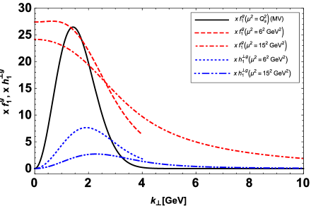
Figure 1: The unpolarized and linearly polarized gluon TMDs as function of $k_{\perp}$ at different scales, at $x$=0.01, using the MV model as input.

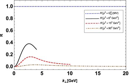
Figure 2: The ratio $R=h_{1}^{\perp g}/f_{1}^{g}$ as function of $k_{\perp}$, at $x=0.01$ for $\mu=6$, 15 and 90 GeV.

With these ingredients, we are ready to perform the numerical study of the evolved gluon TMDs including both unpolarized and linearly polarized gluons. We evolve the gluon TMDs from the saturation scale where the MV results are used as the initial input up to the scales $\mu^{2}=(6\,\text{GeV})^{2}$ and $\mu^{2}=(15\ \text{GeV})^{2}$. As can be seen from Fig. 1, the shape of the unpolarized gluon TMD at low $k_{\perp}$ is significantly changed by evolution. One further observes that the linearly polarized gluon distribution evolves very fast and is suppressed with increasing energy. Since the azimuthal asymmetry induced by the linearly polarized gluon distribution is proportional to the ratio $R=h_{1}^{\perp g}/f_{1}^{g}$, it is instructive to plot this ratio as function of $k_{\perp}$ at different scales in Fig. 2. The dotted blue line represents the ratio computed from the MV model, which is identical to 1 at any value of $k_{\perp}$. That simple relation between the unpolarized gluon TMD and the linearly polarized gluon TMD still holds after taking into account small $x$ evolution Dominguez:2011br , whereas it significantly deviates from it after energy evolution as shown in Fig. 2. The ratio initially grows with increasing $k_{\perp}$ until it reaches a maximal value at a transverse momentum of about two times the saturation scale and then decreases at high transverse momentum. In the typical kinematical region accessible at RHIC, the maximal value of the ratio is slightly less than $0.4$. We also plot a curve for the ratio at the scale $\mu^{2}=(90\,\text{GeV})^{2}$ because it is relevant for studying $\cos 2\phi$ asymmetry for $Z$-jet pair production in $pp$ or $pA$ collisions at LHC. Judging from this curve for $R$, we conclude that it is rather challenging to measure the mentioned azimuthal asymmetry at LHC in this process (and likely in $W$-jet pair production as well). Needless to say, $\gamma^{*}$-jet pair production at lower $\gamma^{*}$ virtuality should be feasible at LHC. There the $x$ values typically are much smaller, but $Q_{s}^{2}$ is only about a factor of 2 larger than at RHIC, requiring $P_{\perp}$ to be larger than say 10 GeV, allowing it to still be selected far below $M_{Z}$. We will also show some results for LHC below.

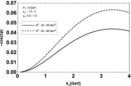
Figure 3: Estimates of the azimuthal asymmetry as function of $k_{\perp}$, calculated at $P_{\perp}=6\ \text{GeV}$, for the different $Q^{2}$ ranges at the center mass energy $\sqrt{s}$=200 GeV. The quark and virtual photon rapidities are integrated over the regions $y_{q}$[1.5, 2] and $y_{\gamma^{*}}$[0.5, 1.5].

The numerical results for the computed azimuthal asymmetry in the different kinematical regions are presented in Figs. 3-5. Here, the azimuthal asymmetry, i.e., the average value of $\text{cos}(2\phi)$, is defined as,

$$\langle\text{cos}(2\phi)\rangle=\frac{\int\frac{d\sigma}{dP.S}d\phi~{}\text{cos}(2\phi)}{\int\frac{d\sigma}{dP.S}d\phi}.$$ (28)

As explained in the above, to avoid dealing with the three scales problem, we choose $Q^{2}$ to be the order of $P_{\perp}^{2}$ which sets the hard scale $\mu^{2}=P_{\perp}^{2}$ when performing energy evolution. We found that the most optimistic rapidity ranges for measuring this azimuthal asymmetry at RHIC energy ($\sqrt{s}$=200 GeV) are $y_{\gamma^{*}}$[1.5, 2], $y_{q}$[0.5, 1.5]. In these rapidity ranges, Fig. 3 shows the asymmetry as function of $k_{\perp}$ for two different $Q^{2}$ ranges at $P_{\perp}=6\ \text{GeV}$. The asymmetry reach a maximal value of 6% for $Q^{2}$[55, 80] around $k_{\perp}=3\ \text{GeV}$. Note that the corresponding longitudinal momentum fraction of the gluon $x$ is in the region [0.008, 0.03] where the MV model results are only borderline justified at best. At LHC the situation is better in this respect, but here we just aim to illustrate the effect of TMD evolution on an observable that in principle probes the linear polarization distribution that becomes maximal at small $x$. Sudakov suppression shows that the observable asymmetry is far from maximal.

For the same rapidity regions, we also plot the asymmetry as function of $P_{\perp}$ with $Q^{2}$ chosen to be $Q^{2}=P_{\perp}^{2}$ and $Q^{2}=\frac{1}{2}P_{\perp}^{2}$, with $k_{\perp}=2.5\text{GeV}$. One sees that there is a relatively mild dependence of the asymmetry on $P_{\perp}$. Fig. 5 shows that the asymmetry grows with increasing virtual photon rapidity. However, a virtual photon rapidity larger than 2 is not reachable at RHIC energy for the kinematical region under consideration. Finally, the asymmetry at LHC energy plotted in Fig. 6 is similar but about a factor 2-3 smaller than that at RHIC.

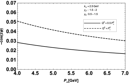
Figure 4: Estimates of the azimuthal asymmetry as function of $P_{\perp}$ with $Q^{2}=P_{\perp}^{2}$ and $Q^{2}=0.5P_{\perp}^{2}$, at $k_{\perp}=2.5\ \text{GeV}$ and $\sqrt{s}$=200 GeV. The quark and virtual photon rapidities are integrated over the regions $y_{q}$[1.5, 2] and $y_{\gamma^{*}}$[0.5, 1.5].

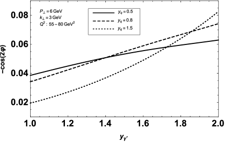
Figure 5: The azimuthal asymmetry evaluated at $k_{\perp}=3\,\text{GeV}$, $P_{\perp}=6\,\text{GeV}$, $\sqrt{s}$=200 GeV, and for the different quark rapidities $y_{q}=0.5,\ 0.8,\ 1.5$, respectively. $Q^{2}$ is integrated over the region [55, 80] $\text{GeV}^{2}$

.

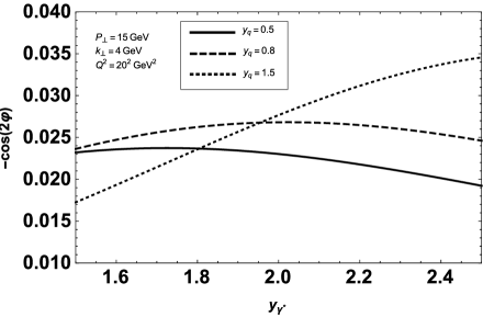
Figure 6: The azimuthal asymmetry evaluated at $k_{\perp}=4\,\text{GeV}$, $P_{\perp}=15\,\text{GeV}$, $Q=20\ \text{GeV}$, $\sqrt{s}$=5.02 TeV and for the different quark rapidities $y_{q}=0.5,\ 0.8,\ 1.5$, respectively.

IV Summary

At small $x$ the linearly polarized gluon TMD is expected to be comparable in size to the unpolarized gluon TMD, reflecting that the Color Glass Condensate can be highly polarized. In the MV model, the linearly polarized gluon TMD saturates the positivity bound for the dipole case, which means that it is in fact identical to the unpolarized gluon TMD. This relation persists under small-$x$ evolution. Such a large effect is very promising for its experimental investigation, especially since the linearly polarized gluon TMD has not been studied experimentally thus far. From a theoretical point of view, the cleanest channel to probe the dipole type linearly polarized gluon TMD is the $\cos 2\phi$ azimuthal asymmetry in virtual photon-jet pair production in $pA$ collisions, which can be studied at RHIC and LHC.

Despite that there is no reason to expect the asymmetry to be small at small $x$, given the maximal size of the linearly polarized gluon TMD, we find that the effect of the linear gluon polarization is strongly suppressed due to TMD evolution effects. In this paper, we have presented numerical estimations of the ratio between the linearly polarized gluon TMD and the unpolarized gluon TMD and of the azimuthal asymmetry taking into account TMD evolution. The ratio after evolution peaks at a transverse momentum on the order of the saturation scale, where its maximal value for instance at scale $\mu^{2}=36\ \text{GeV}^{2}$ is about 0.4 and at $\mu^{2}=M_{Z}^{2}$ only on the few percent level. Despite that the linear gluon TMD enters just once in the $\cos 2\phi$ asymmetry, the Sudakov suppression of the asymmetry is much stronger than the ratio of TMDs would suggest. For the typical kinematic regions accessible at RHIC, the maximal size of the azimuthal asymmetry is found to be around 7%. For such values experimental measurements at RHIC would still seem feasible though. We note that these values do depend on the input distributions we have chosen, but nevertheless we expect these results to give a realistic reflection of the amount of Sudakov suppression for this observable. The situation for LHC is slightly worse, with 2-3% asymmetries, but employing the small-$x$ model as a starting point is more justified in this case. We have also found that the azimuthal asymmetry in jet-$Z/W$ production at LHC is almost completely washed out by the Collins-Soper evolution effect.

In conclusion, the experimental study of this asymmetry at RHIC seems the most promising option and, despite the strong Sudakov suppression, may allow to test the $k_{t}$-resummation formalism in the small-$x$ regime and the theoretical expectation that the Color Glass Condensate state is in fact polarized.

- (1) P. J. Mulders and J. Rodrigues, Phys. Rev. D 63, 094021 (2001) [arXiv:hep-ph/0009343].
- (2) S. Meissner, A. Metz and K. Goeke, Phys. Rev. D 76, 034002 (2007) [arXiv:hep-ph/0703176].
- (3) P. M. Nadolsky, C. Balazs, E. L. Berger and C. -P. Yuan, Phys. Rev. D76, 013008 (2007) [arXiv:hep-ph/0702003].
- (4) S. Mantry and F. Petriello, Phys. Rev. D81, 093007 (2010) [arXiv:0911.4135 [hep-ph]]; and references therein.
- (5) S. Catani and M. Grazzini, Nucl. Phys. B845, 297-323 (2011) [arXiv:1011.3918 [hep-ph]].
- (6) D. Boer, P. J. Mulders and C. Pisano, Phys. Rev. D 80, 094017 (2009) [arXiv:0909.4652 [hep-ph]].
- (7) D. Boer, S. J. Brodsky, P. J. Mulders and C. Pisano, Phys. Rev. Lett. 106, 132001 (2011) [arXiv:1011.4225 [hep-ph]].
- (8) J. -W. Qiu, M. Schlegel and W. Vogelsang, Phys. Rev. Lett. 107, 062001 (2011) [arXiv:1103.3861 [hep-ph]].
- (9) C. Pisano, D. Boer, S. J. Brodsky, M. G. A. Buffing and P. J. Mulders, JHEP 1310, 024 (2013) [arXiv:1307.3417 [hep-ph]].
- (10) P. Sun, B. -W. Xiao and F. Yuan, Phys. Rev. D84, 094005 (2011) [arXiv:1109.1354 [hep-ph]].
- (11) D. Boer, W. J. den Dunnen, C. Pisano, M. Schlegel and W. Vogelsang, Phys. Rev. Lett. 108, 032002 (2012) [arXiv:1109.1444 [hep-ph]].
- (12) J. Wang, C. S. Li, Z. Li, C. P. Yuan and H. T. Li, Phys. Rev. D 86, 094026 (2012) [arXiv:1205.4311 [hep-ph]].
- (13) D. Boer, W. J. den Dunnen, C. Pisano and M. Schlegel, Phys. Rev. Lett. 111, no. 3, 032002 (2013) [arXiv:1304.2654 [hep-ph]].
- (14) S. Catani, L. Cieri, D. de Florian, G. Ferrera and M. Grazzini, Nucl. Phys. B 881, 414 (2014) [arXiv:1311.1654 [hep-ph]].
- (15) D. Boer and W. J. den Dunnen, Nucl. Phys. B 886, 421 (2014) [arXiv:1404.6753 [hep-ph]].
- (16) M. G. Echevarria, T. Kasemets, P. J. Mulders and C. Pisano, JHEP 1507, 158 (2015) [arXiv:1502.05354 [hep-ph]].
- (17) D. Boer and C. Pisano, Phys. Rev. D 86, 094007 (2012) [arXiv:1208.3642 [hep-ph]].
- (18) J. P. Ma, J. X. Wang and S. Zhao, Phys. Rev. D 88, no. 1, 014027 (2013) [arXiv:1211.7144 [hep-ph]].
- (19) W. J. den Dunnen, J. P. Lansberg, C. Pisano and M. Schlegel, Phys. Rev. Lett. 112, 212001 (2014) [arXiv:1401.7611 [hep-ph]].
- (20) G. P. Zhang, Phys. Rev. D 90, no. 9, 094011 (2014) [arXiv:1406.5476 [hep-ph]].
- (21) J. P. Ma and C. Wang, Phys. Rev. D 93, no. 1, 014025 (2016) [arXiv:1509.04421 [hep-ph]].
- (22) L. D. McLerran and R. Venugopalan, Phys. Rev. D 49, 2233 (1994) [arXiv:hep-ph/9309289]; Phys. Rev. D 49, 3352 (1994) [arXiv:hep-ph/9311205].
- (23) A. Metz and J. Zhou, Phys. Rev. D 84, 051503 (2011) [arXiv:1105.1991 [hep-ph]].
- (24) F. Dominguez, J. W. Qiu, B. W. Xiao and F. Yuan, Phys. Rev. D 85, 045003 (2012) [arXiv:1109.6293 [hep-ph]].
- (25) A. Schäfer and J. Zhou, Phys. Rev. D 85, 114004 (2012) [arXiv:1203.1534 [hep-ph]].
- (26) T. Liou, arXiv:1206.6123 [hep-ph].
- (27) E. Akcakaya, A. Schäfer and J. Zhou, Phys. Rev. D 87, no. 5, 054010 (2013) [arXiv:1208.4965 [hep-ph]].
- (28) A. Dumitru, T. Lappi and V. Skokov, Phys. Rev. Lett. 115, no. 25, 252301 (2015) [arXiv:1508.04438 [hep-ph]].
- (29) A. Dumitru and V. Skokov, Phys. Rev. D 94, no. 1, 014030 (2016) [arXiv:1605.02739 [hep-ph]].
- (30) J. C. Collins and D. E. Soper, Nucl. Phys. B 193, 381 (1981) [Erratum-ibid. B 213, 545 (1983)]; Nucl. Phys. B 194, 445 (1982). J. C. Collins, D. E. Soper and G. Sterman, Nucl. Phys. B 250, 199 (1985).
- (31) F. Dominguez, B. W. Xiao and F. Yuan, Phys. Rev. Lett. 106, 022301 (2011) [arXiv:1009.2141 [hep-ph]].
- (32) F. Dominguez, C. Marquet, B. W. Xiao and F. Yuan, Phys. Rev. D 83, 105005 (2011) [arXiv:1101.0715 [hep-ph]].
- (33) P. Kotko, K. Kutak, C. Marquet, E. Petreska, S. Sapeta and A. van Hameren, JHEP 1509, 106 (2015) [arXiv:1503.03421 [hep-ph]].
- (34) A. van Hameren, P. Kotko, K. Kutak, C. Marquet, E. Petreska and S. Sapeta, JHEP 1612, 034 (2016) [arXiv:1607.03121 [hep-ph]].
- (35) A. H. Mueller, B. W. Xiao and F. Yuan, Phys. Rev. Lett. 110, no. 8, 082301 (2013) [arXiv:1210.5792 [hep-ph]].
- (36) A. H. Mueller, B. W. Xiao and F. Yuan, Phys. Rev. D 88, no. 11, 114010 (2013) [arXiv:1308.2993 [hep-ph]].
- (37) J. Zhou, JHEP 1606, 151 (2016) [arXiv:1603.07426 [hep-ph]].
- (38) I. Balitsky and A. Tarasov, JHEP 1510, 017 (2015) [arXiv:1505.02151 [hep-ph]].
- (39) A. Schäfer and J. Zhou, arXiv:1308.4961 [hep-ph].
- (40) J. Zhou, Phys. Rev. D 89, no. 7, 074050 (2014) [arXiv:1308.5912 [hep-ph]].
- (41) D. Boer, M. G. Echevarria, P. Mulders and J. Zhou, Phys. Rev. Lett. 116, no. 12, 122001 (2016) [arXiv:1511.03485 [hep-ph]].
- (42) L. Szymanowski and J. Zhou, Phys. Lett. B 760, 249 (2016) [arXiv:1604.03207 [hep-ph]].
- (43) Y. Hatta, B. W. Xiao and F. Yuan, Phys. Rev. Lett. 116, no. 20, 202301 (2016) [arXiv:1601.01585 [hep-ph]].
- (44) Y. Hagiwara, Y. Hatta and T. Ueda, Phys. Rev. D 94, no. 9, 094036 (2016) [arXiv:1609.05773 [hep-ph]].
- (45) J. Zhou, Phys. Rev. D 94, no. 11, 114017 (2016) [arXiv:1611.02397 [hep-ph]].
- (46) E. Iancu and A. H. Rezaeian, arXiv:1702.03943 [hep-ph].
- (47) D. Boer, S. Cotogno, T. van Daal, P. J. Mulders, A. Signori and Y. J. Zhou, JHEP 1610, 013 (2016) [arXiv:1607.01654 [hep-ph]].
- (48) F. Gelis and J. Jalilian-Marian, Phys. Rev. D 66, 014021 (2002) [hep-ph/0205037].
- (49) T. C. Rogers and P. J. Mulders, Phys. Rev. D 81, 094006 (2010) [arXiv:1001.2977 [hep-ph]].
- (50) A. Schäfer and J. Zhou, Phys. Rev. D 90, no. 3, 034016 (2014) [arXiv:1404.5809 [hep-ph]].
- (51) A. Schäfer and J. Zhou, Phys. Rev. D 90, no. 9, 094012 (2014) [arXiv:1406.3198 [hep-ph]].
- (52) J. Zhou, Phys. Rev. D 92, no. 1, 014034 (2015) [arXiv:1502.02457 [hep-ph]].
- (53) A. H. Mueller, Nucl. Phys. B 558, 285 (1999) [hep-ph/9904404].
- (54) D. Boer, Nucl. Phys. B 874, 217 (2013) [arXiv:1304.5387 [hep-ph]].
- (55) S. M. Aybat and T. C. Rogers, Phys. Rev. D 83, 114042 (2011) [arXiv:1101.5057 [hep-ph]].
- (56) D. Boer, PoS QCDEV 2015, 023 (2015) [arXiv:1510.05915 [hep-ph]].
- (57) J. Collins, L. Gamberg, A. Prokudin, T. C. Rogers, N. Sato and B. Wang, Phys. Rev. D 94, no. 3, 034014 (2016) [arXiv:1605.00671 [hep-ph]].
- (58) K. J. Golec-Biernat and M. Wüsthoff, Phys. Rev. D 59, 014017 (1998) [hep-ph/9807513].