Three-Particle Correlations
in Liquid and Amorphous Aluminium

Abstract

Analysis of three-particle correlations is performed on the basis of simulation data of atomic dynamics in liquid and amorphous aluminium. A three-particle correlation function is introduced to characterize the relative positions of various three particles — the so-called triplets. Various configurations of triplets are found by calculation of pair and three-particle correlation functions. It was found that in the case of liquid aluminium with temperatures $1000\,$K, $1500\,$K, and $2000\,$K the three-particle correlations are more pronounced within the spatial scales, comparable with a size of the second coordination sphere. In the case of amorphous aluminium with temperatures $50\,$K, $100\,$K, and $150\,$K these correlations in the mutual arrangement of three particles are manifested up to spatial scales, which are comparable with a size of the third coordination sphere. Temporal evolution of three-particle correlations is analyzed by using a time-dependent three-particle correlation function, for which an integro-differential equation of type of the generalized Langevin equation is output with help of projection operators technique. A solution of this equation by means of mode-coupling theory is compared with our simulation results. It was found that this solution correctly reproduces the behavior of the time-dependent three-particle correlation functions for liquid and amorphous aluminium.

1 Introduction

At present time the main attention is paid to study the structure of condensed systems, which are in equilibrium or in metastable states [1, 2, 3, 4]. Often, the traditional experimental methods of structural analysis do not allow to correctly identify the presence of some structures in bulk systems due to their small sizes, either low concentrations in the system, or due to relatively short lifetimes. Usually, information about the structure of condensed systems is extracted by using microscopic methods or by methods of X-ray and neutron diffraction. Here, the static structure factor determined from the experimental data is critical quantity, which is related with the pair distribution function, $g(r)$ [2, 4]. At the same time, the pair distribution function $g(r)$ can be determined on the basis of atomic/molecular dynamics simulations, and then it can be compared with experimental data.

In addition, the three-particle correlations has an essential impact for different processes in condensed systems. Thus, an account for three-particle correlations is required to explain the dynamic heterogeneity in liquids [5, 6], to describe of transport properties in chemical reactions [4, 7], to study the structural heterogeneity of materials at mechanical deformations [8, 9], to detect the nuclei of on ordered phase (i.e. crystalline, quasicrystalline) [10, 11], to describe the amorphization of liquids at rapid cooling [2, 4, 12]. Direct evaluation of three-particle correlations by means of experimental measurements is extremely difficult problem [4, 13, 14]. Here, the special methods must be adopted to extract such information [4, 15, 16]. On the other hand, detailed information about the three-particle correlations can be obtained on the basis of atomic/molecular dynamics simulations data. Note that early studies of the three-particle correlations were focused mainly on simple liquids such as the Lennard-Jones fluid, the hard spheres system, and the colloidal systems [4, 17, 18, 19, 20]. In some recent studies, on the basis of data of the molecular dynamics simulation the three-particle correlations were estimated in such systems as carbon nanotubes, electrolytes, metallic melts and alloys [2, 21, 22]. In these studies, the information about three-particle correlations is usually extracted from the time evolution of two and more parameters characterized the positions and trajectories of the particles relative each other.

In the present work, the original method of three-particle structural analysis and evaluation of time-dependent three-particle correlations is proposed, where the arbitrary trajectories of motion of the various three particles (that will be denoted as triplets) are considered. The method allows one to identify the presence of ordered crystalline and “stable” disordered structures, which are difficult to be detected by conventional methods of structural analysis (for example, such as the Voronoi’s tessellation method [23], the Delaunay’s triangulation method [24], the bond-orientational order parameters [3]). The applicability of this method will be demonstrated for the case of the liquid and amorphous aluminium.

2 Simulation Details

We performed the atomic dynamics simulation of liquid and amorphous aluminium. The system contains $N=864$ atoms, located into a cubic simulation cell with periodic boundary conditions in all directions. The interatomic forces are calculated through EAM-potential [25, 26]. The velocities and coordinates of atoms are determined through the integrating Newton’s equations of motion by using Velocity-Verlet algorithm with the time-step $\Delta t=1\,$fs.

Initially, a crystalline sample with fcc lattice and numerical density $\rho=1.23\,\sigma^{-3}$ (or mass density $2300\,$kg/m³) was prepared, where $\sigma=2.86\,$Å is the effective diameter of the aluminium atom. Further, the system was melted to the temperatures $T=1000\,$K, $1500\,$K, and $2000\,$K. The amorphous samples were generated through the fast cooling with the rate $10^{12}\,$K/c of a melt at the temperature $2000\,$K to the temperatures $T=50\,$K, $100\,$K, and $150\,$K (the melting temperature is $T_{m}\simeq 934\,$K). The simulations were performed in NpT-ensemble at constant pressure $p=1\,$atm.

3 Methods

3.1 Three-particle correlation function

Let us consider a system, consisting of $N$ classical particles with same masses $m$, which are located into the simulation cubic cell with a volume $V$. From the geometric point of view, locations of any three particles generate a triangle (i.e. triplet). This triplet is characterized by the area, $S$. Then, the area of $i$th triplet, $S_{i}$, at time $t$ (here $i\in\{1,2,...,N_{T}\}$, $N_{T}$ is the number of all possible triplets in the system) is defined by

$$S_{i}(t)=\left\{l_{i}(t)\cdot[l_{i}(t)-r_{i}^{(12)}(t)]\cdot[l_{i}(t)-r_{i}^{(23)}(t)]\cdot[l_{i}(t)-r_{i}^{(31)}(t)]\right\}^{1/2}.$$ (1)

Here, $l_{i}(t)=[r_{i}^{(12)}(t)+r_{i}^{(23)}(t)+r_{i}^{(31)}(t)]/2$ is the semiperimeter of $i$th triplet; $r_{i}^{(12)}$, $r_{i}^{(23)}$, and $r_{i}^{(31)}$ are the distances between the vertices of $i$th triplet with conditional labels $1$, $2$, and $3$. It follows from Eq.(1) that the area of $i$th triplet, $S_{i}$, takes positive values and values closed to zero. Different triplets can be correlated to the same values $S_{i}$, and the triplets are independent from each other (i.e. have no common vertices) or interconnected (i.e. one or two vertices are mutual). To estimate the quantity $S_{i}$ one vertex of triplet is considered as central (i.e. fixed), relative to which the positions of the other vertices must be defined [see Fig.1].

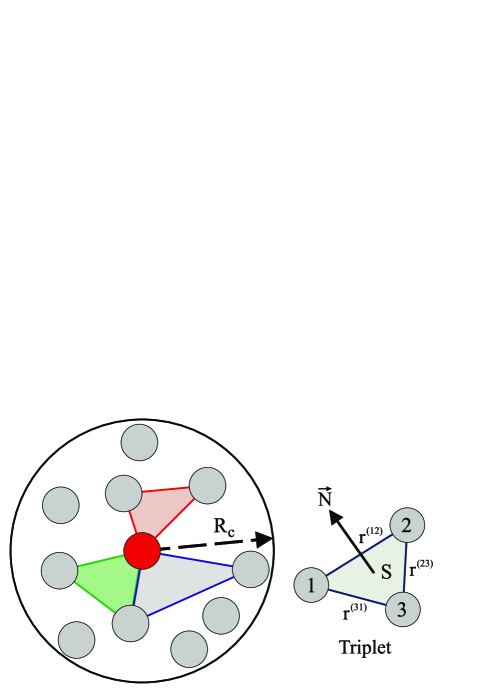
Figure 1: (Color online) Schematic illustration demonstrated the triplets with single and general vertices as well as single triangle with a some area $S$, where the vertices with labels $1$, $2$, and $3$ are presented.

To determine the probability of emergence of the triplets with the area $S$, the three-particle correlation function is introduced

$$g(S)=\frac{1}{N_{T}}\sum_{i=1}^{N_{T}}\delta(S-S_{i}).$$ (2)

Here, the number of the all triplets in the system with $N$ particles is defined by

$$N_{T}=\frac{N(N-1)(N-2)}{6}.$$ (3)

It follows from Eq.(3) that for a system with $N=500$ particles the number of triplets $N_{T}$ is more than $20\,000\,000$. It demonstrates that treatment of simulation results requires significant computing resources. Therefore, at realization of the three-particle structural analysis we can restrict our attention to consider a spherical region with a fixed radius $R_{c}$ in the center of which the main (i.e. fixed) particle of triplet is located. The optimal value of radius $R_{c}$ corresponds to the distance at which the pair correlation function $g(r)$ of considered system ceases to oscillate.

3.2 Dynamics of three-particle correlations

In a system with $N$ particles the coordinates $\vec{q}$ and impulses $\vec{p}$ form a $6N$-dimensional phase space. The time evolution of the system will be defined by the Hamiltonian $H(\vec{q},\vec{p})$, which can be written through the canonical Liouville equation of motion as follows [27]:

$$\frac{dA(t)}{dt}=\{H(\vec{q},\vec{p}),\,A(t)\}=\sum_{i=1}^{N}\left(\frac{\partial H(\vec{q},\vec{p})}{\partial p_{i}}\frac{\partial A(t)}{\partial q_{i}}-\frac{\partial H(\vec{q},\vec{p})}{\partial q_{i}}\frac{\partial A(t)}{\partial p_{i}}\right)$$ (4)

or

$$\frac{dA(t)}{dt}=iLA(t),$$ (5)

where $L$ is the Liouville operator, $\{...\}$ is the Poisson brackets, $A$ is the dynamic variable that obtained from results of simulation. By means of the technique of Zwanzig-Mori’s projection operators

$$\Pi_{0}=\frac{A_{0}(0)\big{\rangle}\big{\langle}A_{0}^{*}(0)}{\left\langle\left|A_{0}(0)\right|^{2}\right\rangle},\,\,P_{0}=1-\Pi_{0},$$ (6)

one obtains from Eq.(5) the following non-Markovian equation [27, 28, 29, 30]:

$$\frac{dF(t)}{dt}=-\Omega_{1}^{2}\int_{0}^{t}M_{1}(\tau)F(t-\tau)d\tau,$$ (7)

where

$$F(t)=\frac{\langle A_{0}^{*}(0)A_{0}(t)\rangle}{\langle|A_{0}(0)|^{2}\rangle}$$ (8)

is the time correlation function;

$$M_{1}(\tau)=\frac{\langle A_{1}^{*}(0)e^{iL_{22}^{0}\tau}A_{1}(0)\rangle}{\langle|A_{1}(t)|^{2}\rangle}$$ (9)

is the first order memory function;

$$\Omega_{1}^{2}=\frac{\langle|A_{1}(0)|^{2}\rangle}{\langle|A_{0}(0)|^{2}\rangle}$$ (10)

is the first-order frequency parameter, and

$$A_{1}(t)=iLA_{0}(t)$$ (11)

is the next dynamics variable. By considering that the Liouville equation for dynamic variable $A_{1}(t)$

$$\frac{dA_{1}(t)}{dt}=iL_{22}^{0}A_{1}(t),$$ (12)

the kinetic integro-differential equation can be obtained for the first-order memory function as follows [27]:

$$\frac{dM_{1}(t)}{dt}=-\Omega_{2}^{2}\int_{0}^{t}M_{2}(\tau)M_{1}(t-\tau)d\tau.$$ (13)

Similarly, a chain of equations can be constructed as

$$\frac{dM_{n-1}(t)}{dt}=-\Omega_{n}^{2}\int_{0}^{t}M_{n}(\tau)M_{n-1}(t-\tau)d\tau,\,n=1,\,2,\,3,...$$ (14)

Here, the $n$th order frequency parameter will be determined as follows [27, 31]:

$$\Omega_{n}^{2}=\frac{\langle|A_{n}(0)|^{2}\rangle}{\langle|A_{n-1}(0)|^{2}\rangle}.$$ (15)

Using the Laplace transformation, $\widetilde{M}_{n}(s)=\int_{0}^{\infty}e^{-st}M_{n}(t)dt$ (where $s=i\omega$), the chain of equations (14) can be rewritten as a continued fraction [27]

$$\widetilde{F}(s)=\frac{1}{\displaystyle s+\frac{\Omega_{1}^{2}}{\displaystyle s+\frac{\Omega_{2}^{2}}{\displaystyle s+\ldots}}}.$$ (16)

From Eq.(14) one obtains [27, 31]

$$\ddot{F}(k,t)+\Omega_{1}^{2}(k)F(k,t)+\Omega_{2}^{2}(k)\int_{0}^{t}M_{2}(k,t-\tau)\dot{F}(k,\tau)d\tau=0,$$ (17)

where $k=|\vec{k}|$ is the wave number [2, 28]. By using the key condition of the mode-coupling theory [27, 31]

$$\Omega_{2}^{2}(k)M_{2}(k,t)=\varphi(k)\delta(t)+\Omega_{1}^{2}(k)\left[\upsilon_{1}F(k,t)+\upsilon_{2}F(k,t)^{p}\right],$$ (18)

the Eq.(17) can be rewritten in the form

$$\ddot{F}(k,t)+\Omega_{1}^{2}(k)F(k,t)+\varphi(k)\dot{F}(k,t)\delta(t)+$$

$$+\Omega_{1}^{2}(k)\int_{0}^{t}\left[\upsilon_{1}F(k,t-\tau)+\upsilon_{2}F(k,t-\tau)^{p}\right]\dot{F}(k,\tau)d\tau=0.$$ (19)

Here, $\Omega_{1}(k)$ and $\varphi(k)$ are the frequency parameters, $\delta(t)$ is the Dirac’s delta function, $\upsilon_{1}\geq 0$, $\upsilon_{2}\geq 0$ ($\upsilon_{1}+\upsilon_{2}\neq 0$) are the weight of the corresponding contributions, the parameter $p>1$ can be fractional. The exact solution of Eq.(19) will be defined through the frequency parameters $\Omega_{1}(k)$, $\varphi(k)$ as well as through the characteristics $\upsilon_{1}$, $\upsilon_{2}$, and $p$ [32].

A numerical solution of integro-differential Eq.(19) can be found from [32]:

$$z_{n}+\Omega_{1}^{2}x_{n}+\Omega_{1}^{2}\tau\sum_{i=0}^{n}\left[\upsilon_{1}x_{i}+\upsilon_{2}x_{i}^{p}\right]z_{n-i}=0,$$ (20)

$$y_{n+1}=y_{n}+\tau z_{n},$$ (21)

$$x_{n+1}=x_{n}+\tau y_{n+1}.$$ (22)

Let us take the quantity

$$\vec{s}_{j}(t)=\frac{\mu_{j}S_{j}(t)\vec{N}_{j}}{\sigma},\,\,j=1,2,...,N_{T}$$ (23)

as a dynamical variable. If the value $A_{0}=\vec{s}_{j}(t)$ is taken as initial dynamical variable [see Eq.(6)], then the time correlation function will be defined as

$$F_{T}(k,t)=\frac{1}{N_{T}}\sum_{j=1}^{N_{T}}\exp\left[-i\vec{k}(\vec{s}_{j}(t)-\vec{s}_{j}(0))\right],$$ (24)

and $x_{n}=F_{T}(k,t)$, $y_{n}=\dot{F}_{T}(k,t)$, $z_{n}=\ddot{F}_{T}(k,t)$, where $\tau=0.01\,$fs, while initial conditions in Eq.(20) are $F_{T}(k,t=0)=1$ and $\dot{F}_{T}(k,t=0)=0$ [32]. Here, $S_{j}(t)$ is the area of $j$th triplet at time $t$, $\vec{N}_{j}=n_{j1}\vec{e_{x}}+n_{j2}\vec{e_{y}}+n_{j3}\vec{e_{z}}$ is the vector of normal to the plane of this triangle [see illustration in Fig.1], $\mu_{j}=\pm[n_{j1}^{2}+n_{j2}^{2}+n_{j3}^{2}]^{-1/2}$ is the normalization constant determined by a sign of parameter $n_{j4}$ from equation of the plane $n_{j1}x+n_{j2}y+n_{j3}z+n_{j4}=0$, which connects of vertices of $j$th triplet. At $n_{j4}>0$ we have a value $\mu_{j}<0$, otherwise we have a value $\mu_{j}>0$.

4 Results and Discussions

4.1 Behavior of single triplet

The time dependent area of a triplet is evaluated at different temperatures. Thus, in Fig.2 (top panel) it is shown the time-dependent area of a triplet $S(t)$ in liquid aluminium at temperature $1000\,$K. It can be seen that the quantity $S(t)$ takes the values in the range $0.25\,$nm${}^{2}<S<1\,$nm². The evolution of $S(t)$ in the case of liquid aluminium is characterized by the high-frequency fluctuations of a relatively small amplitude, which are originated due to collective motion of atoms. The low-frequency fluctuations with a relatively large amplitude define a main trend of $S(t)$, and they defined by transition to the diffusive motion of particles, when an atom or several atoms leave a nearest environment.

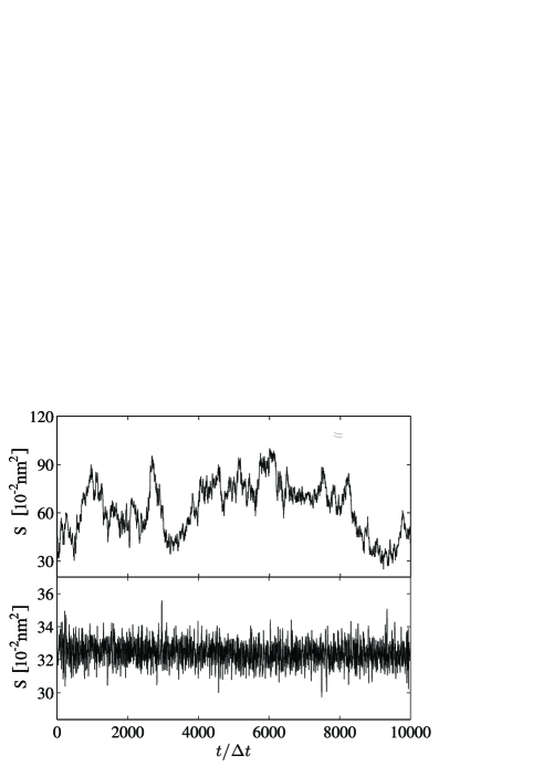
Figure 2: Time-dependent area of a triplet in atomic dynamics of aluminium. Top panel: liquid aluminium at the temperature $1000$ K. Bottom panel: amorphous aluminium at the temperature $100$ K.

Fig.2 (bottom panel) represents the time-dependent area of a triplet in amorphous aluminium at temperature $T=100\,$K. Contrasted to the liquid, the diffusive regime of $S(t)$ is not observed, that is due to extremely low mobility of atoms. The fluctuations with relatively small amplitude are seen; wherein the area $S(t)$ takes the values within a narrow range $0.29\,$nm${}^{2}<S<0.36\,$nm². These fluctuations is caused by vibrations of atoms in a surrounded of “neighbors”.

4.2 Features of three-particle correlations

The distribution function $g(S)$ was computed by Eq.(2) for the liquid and amorphous systems, and those triplets were considered, only which located within a sphere of the radius $R_{c}=3\,\sigma$. Also, the pair distribution function was determined as follows [2, 33, 34]:

$$g(r)=\frac{V}{4\pi r^{2}N}\sum_{i=1}^{N}\left\langle\frac{\Delta n_{i}(r)}{\Delta r}\right\rangle,$$ (25)

where $\Delta n_{i}(r)$ is the probability to find the pair of the atoms separated by the distance $r$. For convenience, the distances between the atoms we will measure in the units of $\sigma$ and the area of triplet in the units of $\sigma^{2}$ (here, $\sigma=2.86\,$Å).

Fig.3 shows the curves $g(S)$ and $g(r)$ for liquid aluminium at temperatures $1000\,$K, $1500\,$K, and $2000\,$K. As seen the pair distribution function $g(r)$ of liquid aluminium has oscillations and contains the maxima at distances $r=r_{m1}^{(L)}$, $r_{m2}^{(L)}$, $r_{m3}^{(L)}$, and $r_{m4}^{(L)}$, which characterize the correlation lengths. The estimated inter-particle distances $r=r_{m1}^{(L)}$, $r_{m2}^{(L)}$, $r_{m3}^{(L)}$, and $r_{m4}^{(L)}$ are given in Table 1. The undistinguished maximum at $r\simeq r_{m4}^{(L)}$ is indication that the pair correlations are practically absent at large distances. For the reason that both the functions $g(S)$ and $g(r)$ correspond to the same system, it is quite reasonable to assume that the maxima in function $g(S)$, located at $S=S_{m1}^{(L)}$ and $S_{m2}^{(L)}$, are associated with the triplets, in which the distances between pairs of atoms correspond to correlation lengths $r_{m1}^{(L)}$, $r_{m2}^{(L)}$, $r_{m3}^{(L)}$, and $r_{m4}^{(L)}$. Then, the different possible configurations of three atoms can be selected, where the atoms that form these triplets are remote to the distances $r=r_{m1}^{(L)}$, $r_{m2}^{(L)}$, $r_{m3}^{(L)}$, and $r_{m4}^{(L)}$. As a result of such selection, five different widespread configurations appear in liquid aluminium, which are depicted in Fig.4 with labels CL1, CL2,…, CL5.

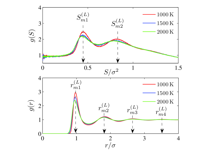
Figure 3: (Color online) Three-particle correlation function $g(S)$ (top panel) and pair distribution function $g(r)$ (bottom panel), obtained for liquid aluminium at temperatures $1000$ K, $1500$ K, and $2000$ K. The positions of main maxima of the functions $g(S)$ and $g(r)$ are indicated by arrows.

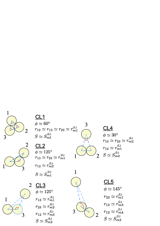
Figure 4: (Color online) Triplets which appear in liquid aluminium and correspond to the main maxima of the functions $g(S)$ and $g(r)$. The circles mark the atoms. The lines mark the distances $r_{12}$, $r_{23}$, and $r_{13}$ between the atoms. Here, $\phi$ is the angle between two straight lines, which connect the vertices of the triangle.

From analysis of simulation data, it follows that the triplets with configurations CL1 and CL2, which correspond to the maximum at $S_{m1}^{(L)}$ in the function $g(S)$ that also give impact to the main maxima of the function $g(r)$ at $r_{m1}^{(L)}$ and $r_{m2}^{(L)}$. In this case, a mutual arrangement of three atoms covers a spatial scale, which are comparable with size of the first and second coordination spheres. Also, the presence of triplets with configurations CL1 and CL2 is observed in other model liquids [4]. So, Zahn et al. observed the triplets with inter-particle distances $r\simeq 1.0\,\sigma$ and $r\simeq 1.9\,\sigma$ (i.e. with configurations similar to CL1 and CL2, where $r=r_{m1}^{(L)}\simeq 0.96\,\sigma$ and $r_{m2}^{(L)}\simeq 1.82\,\sigma$) in two-dimensional colloidal liquid, where three-particle correlation functions were calculated from particle configurations (see Fig.2 and Fig.4 in Ref.[4]). The triplets CL3, CL4, and CL5 that correspond to the maximum of function $g(S)$ at $S_{m2}^{(L)}$, are usually involved to formation of maxima of the function $g(r)$ at $r_{m3}^{(L)}$ and $r_{m4}^{(L)}$. Remarkable that the structure of the system can be restored by connecting the different configurations CL1, CL2, CL3, CL4, and CL5.

Fig.5 represents the functions $g(S)$ and $g(r)$ for amorphous system at temperatures $50\,$K, $100\,$K, and $150\,$K. Five pronounced maxima are detected for $g(S)$, and eight maxima are most pronounced for the function $g(r)$. As seen from Fig.5 (top panel), the function $g(S)$ contain the maxima at $S=S_{m1}^{(A)}$, $S_{m2}^{(A)}$, $S_{m5}^{(A)}$, as $S_{m3}^{(A)}$ and $S_{m4}^{(A)}$, which are not observed for liquid system. The estimated inter-particle distances, which correspond to positions of maxima of the functions $g(S)$ and $g(r)$, are given in Table 2.

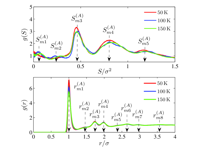
Figure 5: (Color online) Three-particle correlation function $g(S)$ (top panel) and pair distribution function $g(r)$ (bottom panel), obtained for amorphous aluminium at temperatures $50\,$K, $100\,$K, and $150\,$K.

In the case of amorphous aluminium, various triplets are detected, where twelve configurations can be chosen as widespread, which depicted in Fig.6 with labels CA1, CA2,…, CA12. Wherein, the most of the configurations except of CA1, CA3, and CA4 cover the spatial scale, which exceeds the size of the second coordination sphere. The presence of maxima at small areas $S$ (for example, the maxima at $S=S_{m1}^{(A)}$ and $S_{m2}^{(A)}$), which correspond to CA1 and CA2, can be indication of structural ordering, as well as evidence of the presence of quasi-ordered structures. At the same time, the configurations CA1 and CA2 together with CA3 and CA4 generate the main maximum of the function $g(r)$ at the distance $r=r_{m1}^{(A)}$. The formation of triples CA5, CA6,…, CA9, that correspond to the maxima of function $g(S)$ at $S=S_{m3}^{(A)}$ and $S_{m4}^{(A)}$, leads to splitting of second maximum of the function $g(r)$. The configurations CA2, CA4, and CA11 participate to formation of the maximum of $g(r)$ at $r=r_{m2}^{(A)}$, and give impact to the maxima of the three-particle correlation function $g(S)$ at $S=S_{m2}^{(A)}$, $S_{m3}^{(A)}$, and $S_{m5}^{(A)}$. The presence of maximum in the function $g(S)$ at $S=S_{m5}^{(A)}$ is due to the triplets CA10, CA11,…, CA12, the number of which is negligible.

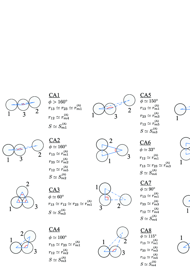
Figure 6: (Color online) Configurations of triplets in the amorphous aluminium, which involve in the formation of the main maxima of the functions $g(S)$ and $g(r)$.

The configurations CL1, CL2,…, CL5 and CA1, CA2,…, CA12 appear because the atoms that form these triplets are surrounded by neighbors, which slow down their motion – so-called cage effect. According to effective neighborhood model proposed by Vorselaars et al., the cage effect occurs in liquids and glasses, where the particles are trapped in a local energy minimum [6]. Namely, a single particle at motion jumps from one cage to another cage (i.e. from one local energy minimum to another local energy minimum) [6]. In the case of aluminium atoms with configurations, which are depicted in Fig.4 and Fig.6, the jumps between different cages lead to transitions between various triplets. Usually, these transitions occur between triplets with similar configurations, for example, between CL1 and CL2, between CL3 and CL4 in the case of liquid aluminium as well as between CA1 and CA2, between CA3 and CA4, between CA6 and CA10, between CA7 and CA8 in the case of amorphous aluminium. Unlike liquid, in the amorphous system the transitions between the triplets of different configurations occur very slowly, where the jumps of atoms between different cages occur for a long time due to the high viscosity.

4.3 Time-dependent three-particle correlations

The analysis of the time-dependent three-particle correlations is also done by means of the time correlation function $F_{T}(k,t)$, defined by Eq.(24). As an example, the function $F_{T}(k,t)$ obtained for liquid and amorphous aluminium at different temperatures is presented in Fig.7. The calculations were performed at fixed value of the wave number $k=4.6\,$Å^-1. We note that the behavior of the function $F_{T}(k,t)$ is similar to behavior of incoherent scattering function $F(k,t)$ [35]. The function $F_{T}(k,t)$ demonstrates the fast decay to zero in the case of liquid system, that is caused with attenuation of three-particle correlations. The rate of attenuation is expected to be correlated with the structural relaxation time. In the case of amorphous aluminium at temperatures $50\,$K, $100\,$K, and $150\,$K, the function $F_{T}(k,t)$ is characterized by more complex shape.

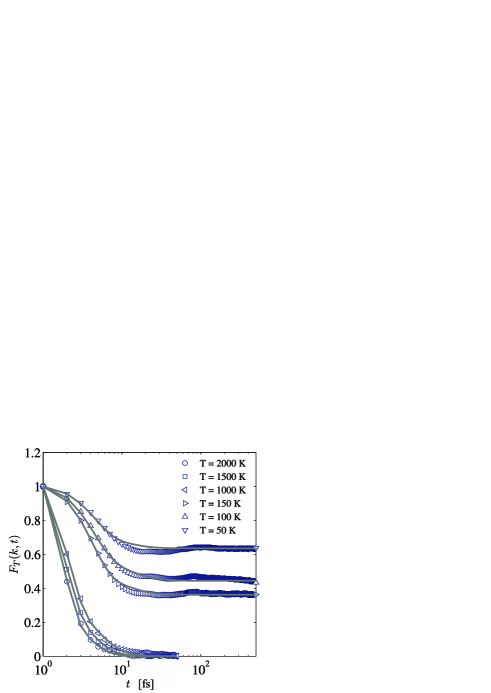
Figure 7: (Color online) Three-particle correlation function $F_{T}(k,t)$ obtained for aluminium at various temperatures and at wave number $k=4.6$ Å^-1. The solid lines mark the theoretical results; symbols depict results of simulations.

On the other hand, the function $F_{T}(k,t)$ was computed by Eq.(19) on the basis of simulation results at $k=4.6\,$Å^-1 and the temperatures $T=50\,$K, $100\,$K, $150\,$K, $1000\,$K, $1500\,$K, and $2000\,$K. Then, the Eq.(19) was solved numerically according to scheme (20)–(24), while the parameters $\upsilon_{1}$, $\upsilon_{2}$, $\Omega_{1}^{2}$, $p$ were taken as adjustable. The values of the parameters are given in Table 3. As can be seen from Fig.7, the theory with Eq.(19) reproduces the behavior of function $F_{T}(k,t)$ at all considered temperatures. Further, for the case of amorphous system, the theory allows one to reproduce the emergence of plateau in function $F_{T}(k,t)$. The frequency parameter, $\Omega_{1}^{2}$, takes the relatively small values $3.3\times 10^{25}\,$s${}^{-2}\leq\Omega_{1}^{2}\leq 9.8\times 10^{25}\,$s^-2 for amorphous system and large values $64\times 10^{25}\,$s${}^{-2}\leq\Omega_{1}^{2}\leq 130\times 10^{25}\,$s^-2 for liquid system. Here, the increase of the parameter $\Omega_{1}^{2}$ with temperature can be due to increase of transition rate between triplets of various configurations.

5 Conclusion

In the present work, the analysis of the three-particle correlations in many-particle systems is suggested. By atomic dynamics simulation of liquid and amorphous aluminium, the applicability of the proposed method of three-particle structural analysis is demonstrated to identify the structures, which are generated by various triplets. By applying the calculation of the pair and three-particle distribution functions, the triplets of various configurations are found. It has been shown that these triplets, which are formed due to particle correlations can cover the spatial scales, which are comparable with sizes of the second and third coordination spheres. On the other hand, it was found that the time evolution of the three-particle correlations in liquid and amorphous aluminium can be recovered from transition between triplets of various configurations. Then, it is shown that the time-dependent three-particle correlations in these systems are reproducible by the integro-differential equation (19). Here, an agreement between theoretical results and our atomic dynamics simulation data is observed.

Tables

Table 1: Inter-particle distances $r_{m1}^{(L)}$, $r_{m2}^{(L)}$, $r_{m3}^{(L)}$, and $r_{m4}^{(L)}$ (in units $\sigma$), as well as the areas $S_{m1}^{(L)}$ and $S_{m2}^{(L)}$ (in units $\sigma^{2}$), which correspond to positions of the main maxima of the functions $g(r)$ and $g(S)$ in the case of liquid aluminium. The errors in the values are estimated to be less than $5$%.

$T,\,$K	$r_{m1}^{(L)}$	$r_{m2}^{(L)}$	$r_{m3}^{(L)}$	$r_{m4}^{(L)}$	$S_{m1}^{(L)}$	$S_{m2}^{(L)}$
$1000$	$0.969$	$1.841$	$2.661$	$3.535$	$0.45$	$0.823$
$1500$	$0.962$	$1.822$	$2.654$	$3.532$	$0.44$	$0.803$
$2000$	$0.955$	$1.815$	$2.647$	$3.528$	$0.43$	$0.797$

Table 2: Inter-particle distances $r_{m1}^{(A)},\,r_{m2}^{(A)},...,\,r_{m8}^{(A)}$ (in units $\sigma$) and the areas $S_{m1}^{(A)},\,S_{m2}^{(A)},...,\,S_{m5}^{(A)}$ (in units $\sigma^{2}$), which correspond to positions of the main maxima of the functions $g(r)$ and $g(S)$ in the case of amorphous aluminium. The errors in the values are estimated to be less than $8$%.

$T,\,$K	$r_{m1}^{(A)}$	$r_{m2}^{(A)}$	$r_{m3}^{(A)}$	$r_{m4}^{(A)}$	$r_{m5}^{(A)}$	$r_{m6}^{(A)}$	$r_{m7}^{(A)}$	$r_{m8}^{(A)}$
$50$	$1.0$	$1.472$	$1.731$	$1.983$	$2.381$	$2.657$	$2.962$	$3.612$
$100$	$1.0$	$1.465$	$1.738$	$1.982$	$2.379$	$2.654$	$2.961$	$3.609$
$150$	$1.0$	$1.455$	$1.734$	$1.982$	$2.378$	$2.651$	$2.958$	$3.605$
$T,\,$K	$S_{m1}^{(A)}$	$S_{m2}^{(A)}$	$S_{m3}^{(A)}$	$S_{m4}^{(A)}$	$S_{m5}^{(A)}$
$50$	$0.02$	–	$0.455$	$0.804$	$1.17$
$100$	$0.06$	$0.24$	$0.471$	$0.811$	$1.23$
$150$	$0.08$	$0.28$	$0.458$	$0.851$	$1.19$

Table 3: Numerical values of the parameters $\upsilon_{1}$, $\upsilon_{2}$, $\Omega_{1}^{2}$, and $p$ of the integro-differential Eq.(19) obtained from fit of numerical solution of Eq.(19) to simulation results.

$T,\,$K	$\upsilon_{1}$	$\upsilon_{2}$	$\Omega_{1}^{2}$, $\times 10^{25}\,$s-2	$p$
$50$	$1.531$	$13.43$	$3.3$	$1.62$
$100$	$1.232$	$9.334$	$6.5$	$1.52$
$150$	$0.934$	$8.415$	$9.8$	$1.45$
$1000$	$0.815$	$1.873$	$64$	$2.32$
$1500$	$0.795$	$1.721$	$98$	$2.0$
$2000$	$0.713$	$1.634$	$130$	$1.96$

References

- [1] D. Kashchiev, Nucleation: Basic Theory with Applications, Butterworth-Heinemann, Oxford, 2000.
- [2] N.H. March, M.P. Tosi, Atomic dynamics in liquids, Dover, New-York, 1991.
- [3] P. Steinhardt, D. Nelson, and M. Ronchetti, Bond-orientational order in liquids and glasses, Phys. Rev. B. 28 (1983) 784-805. https://doi.org/10.1103/PhysRevB.28.784
- [4] K. Zahn, G. Maret, C. Ruß, H.H. von Grunberg, Three-Particle Correlations in Simple Liquids, Phys. Rev. Lett. 91 (2003) 115502 1-4. https://doi.org/10.1103/PhysRevLett.91.115502
- [5] M.M. Hurley, P. Harrowell, NonGaussian behavior and the dynamical complexity of particle motion in a dense two dimensional liquid, J. Chem. Phys. 105 (1996) 10521-10526. http://dx.doi.org/10.1063/1.472941
- [6] B. Vorselaars, A.V. Lyulin, K. Karatasos, M.A.J. Michels, Non-Gaussian nature of glassy dynamics by cage to cage motion, Phys. Rev. E. 75 (2007) 011504 1-6. https://doi.org/10.1103/PhysRevE.75.011504
- [7] T. Lazaridis, Solvent Reorganization Energy and Entropy in Hydrophobic Hydration, J. Phys. Chem. B. 104 (2000) 4964-4979. http://pubs.acs.org/doi/pdf/10.1021/jp994261a
- [8] H. Wang, M. P. Lettinga, and J. K. G. Dhont, Microstructure of a near-critical colloidal dispersion under stationary shear flow, J. Phys. Condens. Matter. 14 (2002) 7599-7615. http://dx.doi.org/10.1088/0953-8984/14/33/304
- [9] A.V. Mokshin, B.N. Galimzyanov, J.-L. Barrat, Extension of classical nucleation theory for uniformly sheared systems, Phys. Rev. E. 87 (2013) 062307 1-5. https://doi.org/10.1103/PhysRevE.87.062307
- [10] M. Dzugutov, Formation of a Dodecagonal Quasicrystalline Phase in a Simple Monatomic Liquid, Phys. Rev. Lett. 70 (1993) 2924-2927. https://doi.org/10.1103/PhysRevLett.70.2924
- [11] J.P.K. Doye, D.J. Wales, Polytetrahedral Clusters, Phys. Rev. Lett. 86 (2001) 5719-5722. https://doi.org/10.1103/PhysRevLett.86.5719
- [12] M. Tokuyama, Similarities in diversely different glass-forming systems, Physica A. 378 (2007) 157-166. http://dx.doi.org/10.1016/j.physa.2006.12.047
- [13] O.S. Vaulina, O.F. Petrov, V.E. Fortov, A.V. Chernyshev, A.V. Gavrikov, and O.A. Shakhova, Three-Particle Correlations in Nonideal Dusty Plasma, Phys. Rev. Lett. 93 (2004) 035004 1-4. https://doi.org/10.1103/PhysRevLett.93.035004
- [14] G.L. Ma, Y.G. Ma, S. Zhang, X.Z. Cai, J.H. Chen, Z.J. He, H.Z. Huang, J.L. Long, W.Q. Shen, X.H. Shi, C. Zhong, J.X. Zuo, Three-particle correlations from parton cascades in Au + Au collisions, Phys. Lett. B. 647 (2007) 122-127. http://dx.doi.org/10.1016/j.physletb.2007.02.008
- [15] P.A. Egelstaff, D.I. Page, and C.R.T. Heard, Experimental Study of the Triplet Correlation Function for simple liquids, Phys. Lett. A. 30 (1969) 376-377. http://dx.doi.org/10.1088/0022-3719/4/12/002
- [16] W. Montfrooij, L.A. de Graaf, P.J. van der Bosch, A.K. Soper, and W.S. Howells, Density and temperature dependence of the structure factor of dense fluid helium, J. Phys. Condens. Matter. 3 (1991) 4089-4096. http://dx.doi.org/10.1088/0953-8984/3/22/018
- [17] B.J. Alder, Triplet Correlations in Hard Spheres, Phys. Rev. Lett. 12 (1964) 317-319. https://doi.org/10.1103/PhysRevLett.12.317
- [18] S. Gupta, J.M. Haile, and W.A. Steele, Use of Computer Simulation to Determine the Triplet Distribution Function in Dense Fluids, Chem. Phys. 72 (1982) 425-440. http://dx.doi.org/10.1016/0301-0104(82)85138-0
- [19] W.J. McNeil, W.G. Madden, A.D.J. Haymet, and S.A. Rice, Triplet correlation functions in the LennardJones fluid: Tests against molecular dynamics simulations, J. Chem. Phys. 78 (1983) 388-398. http://dx.doi.org/10.1063/1.444514
- [20] P. Attard, G. Stell, Three-particle correlations in a hard-sphere fluid, Chem. Phys. Lett. 189 (1992) 128-132. http://dx.doi.org/10.1016/0009-2614(92)85110-V
- [21] T. Gaskell, An improved description of three-particle correlations in liquids and a modified Born-Green equation, J. Phys. C: Solid State Phys. 21 (1988) 1-6. http://dx.doi.org/10.1088/0022-3719/21/1/003
- [22] T. Deilmann, M. Druppel, M. Rohlfing, Three-particle correlation from a Many-Body Perspective: Trions in a Carbon Nanotube, Phys. Rev. Lett. 116 (2016) 196804 1-6. https://doi.org/10.1103/PhysRevLett.116.196804
- [23] N.N. Medvedev, The Voronoi-Delaunay method for non-crystalline structures, Siberian Branch of RAS, Novosibirsk, 2000.
- [24] D. Lee, B. Schachter, Two Algorithms for Constructing a Delaunay Triangulation, Int. Jour. Comp. and Inf. Sc. 9 (1980) 219-242. http://link.springer.com/article/10.1007/BF00977785
- [25] F. Ercolessi, J.B. Adams, Interatomic Potentials from First-Principles Calculations: The Force-Matching Method, Europhys. Lett. 26 (1994) 583-588. http://dx.doi.org/10.1209/0295-5075/26/8/005
- [26] J.M. Winey, A. Kubota, Y.M. Gupta, A thermodynamic approach to determine accurate potentials for molecular dynamics simulations: thermoelastic response of aluminum, Modelling Simul. Mater. Sci. Eng. 17 (2009) 055004 1-14. http://dx.doi.org/10.1088/0965-0393/17/5/055004
- [27] A.V. Mokshin, A.V. Chvanova and R.M. Khusnutdinoff, Mode-Coupling Approximation in Fractional-Power Generalization: Particle Dynamics in Supercooled Liquids and Glasses, Theor. Math. Phys. 171 (2012) 541-552. http://link.springer.com/article/10.1007/s11232-012-0052-3
- [28] R. Zwanzig, Nonequilibrium statistical mechanics, Oxford Univ. Press, Oxford, 2001.
- [29] R.M. Yulmetyev, A.V. Mokshin, P.Hänggi, Universal approach to overcoming nonstationarity, unsteadiness and non-Markovity of stochastic processes in complex systems, Physica A. 345 (2005) 303-325. http://dx.doi.org/10.1016/j.physa.2004.07.001
- [30] R. Yulmetyev, R. Khusnutdinoff, T. Tezel, Y. Iravul, B. Tuzel, P. Hänggi, The study of dynamic singularities of seismic signals by the generalized Langevin equation, Physica A. 388 (2009) 3629-3635. http://dx.doi.org/10.1016/j.physa.2009.05.010
- [31] A.V. Mokshin, Self-Consistent Approach to the Description of Relaxation Processes in Classical Multiparticle Systems, Theor. Math. Phys. 183 (2015) 449-477. http://link.springer.com/article/10.1007/s11232-015-0274-2
- [32] R.M. Khusnutdinoff, A.V. Mokshin, Local Structural Order and Single-Particle Dynamics in Metallic Glass, Bulletin of the RAS: Physics. 74 (2010) 640-643. http://link.springer.com/article/10.3103/S1062873810050163
- [33] P.H. Poole, C. Donati, S.C. Glotzer, Spatial correlations of particle displacements in a glass-forming liquid, Physica A. 261 (1998) 51–59. http://dx.doi.org/10.1016/S0378-4371(98)00376-8
- [34] R.M. Khusnutdinoff, A.V. Mokshin, Vibrational features of water at the low-density/high-density liquid structural transformations, Physica A. 391 (2012) 2842-2847. http://dx.doi.org/10.1016/j.physa.2011.12.037
- [35] J.P. Hansen, I. R. McDonald, Theory of Simple Liquids, Academic Press, London, 2006.