A theorem about two-body decay and its application for a doubly-charged boson $H^{\pm\pm}$ going to $\tau^{\pm}\tau^{\pm}$

Abstract

In a general decay chain $A\to B_{1}B_{2}\to C_{1}C_{2}\ldots$, we prove that the angular correlation function $I(\theta_{1},\theta_{2},\phi_{+})$ in the decay of $B_{1,2}$ is irrelevant to the polarization of the mother particle $A$ at production. This guarantees that we can use these angular distributions to determine the spin-parity nature of $A$ without knowing its production details. As an example, we investigate the decay of a potential doubly-charged boson $H^{\pm\pm}$ going to same-sign $\tau$ lepton pair.

I introduction

After the discovery of the higgs boson $h(125)$ higgs_atlas ; higgs_cms , we are more and more interested in searching for high-mass particles, such as doubly-charged higgs bosons hpp_atlas1 ; hpp_atlas2 ; hpp_cms , denoted by $H^{\pm\pm}$. Once we observe any unknown particle, it is crucial to determine its spin-parity ($J^{P}$) nature to discriminate different theoretic models. A good means is to study the angular distributions in a decay chain where the unknown particle is involved nelson1 ; nelson2 ; nelson3 ; spin_qi ; spin_mi . For the Standard Model (SM) higgs, its spin-parity nature can be probed in the decay modes $h(125)\to W^{+}W^{-}/ZZ/\tau^{+}\tau^{-}$ JP_atlas1 ; JP_atlas2 ; JP_atlas3 ; JP_cms1 ; JP_cms2 . The validity of this method relies on that the correlation of the decay planes of $W/Z/\tau$ does not depend upon the polarization of $h(125)$ at production. This is proved in a general case in this paper. As an example, we also investigate the decay $H^{++}\to\tau^{+}\tau^{+}$, where the spin-statistic relation provides more interesting constraints as the final state is two identical fermions.

II Proof of the theorem

Let us consider a general decay chain $A\to B_{1}B_{2}$ with $B_{1}\to C_{1}X_{1}$ and $B_{2}\to C_{2}X_{2}$, where $B_{1}$ and $B_{2}$ can be different particles and $C_{1}X_{1}$ and $C_{2}X_{2}$ can be different decay modes even if $B_{1}$ and $B_{2}$ are identical particles. Here we prove a theorem, which states that the angular correlation function $I(\theta_{1},\theta_{2},\phi_{+})$ (defined in Eq. 9) in the decay of the daughter particles $B_{1,2}$ is independent upon the polarization of the mother particle $A$. Let $\phi_{+}$ denote the angle between two decay planes $B_{i}\to C_{i}X_{i}$ ($i=1,2$). Therefore, we can measure the $\phi_{+}$ distribution to determine the spin-parity nature of the mother particle $A$ without knowing its production details .

Before calculating the amplitude, we introduce the definition of the coordinate system to describe the decay chain as illustrated in Fig. 1. For the decay $A\to B_{1}B_{2}$, we take the flight direction of $A$ as the $+z$ axis (if it is still, we take its spin direction as the $+z$ direction), denoted by $\hat{z}(A)$. $\theta$ and $\phi$ are the polar angle and azimuthal angle of $B_{1}$ in the center-of-mass (c.m.) frame of $A$. For the decay $B_{1}\to C_{1}X_{1}$, we take the flight direction of $B_{1}$ in the c.m. frame of $A$ as the $+z$ axis, denoted by $\hat{z}(B_{1})$ and the direction of $\hat{z}(A)\times\hat{z}(B_{1})$ as the $+y$ axis, denoted by $\hat{y}(B_{1})$. The $+x$ axis in this decay system is then defined as $\hat{y}(B_{1})\times\hat{z}(B_{1})$. $\theta_{1}$ and $\phi_{1}$ are the polar angle and azimuthal angle of $C_{1}$ in the c.m. frame of $B_{1}$. The same set of definitions holds for the decay $B_{2}\to C_{2}X_{2}$. $\phi_{+}$ is defined in Eq. 1. It represents the angle between the two decay planes of $B_{i}\to C_{i}X_{i}$ ($i=1,2$). Here $\phi_{1}$, $\phi_{2}$ and $\phi_{+}$ are constrained in the range $[0,2\pi)$.

$$\phi_{+}\equiv\left\{\begin{array}[]{ll}\phi_{1}+\phi_{2}\>,&\text{if}\>\phi_{1}+\phi_{2}<2\pi\\ \phi_{1}+\phi_{2}-2\pi\>,&\text{if}\>\phi_{1}+\phi_{2}>2\pi\\ \end{array}\right.$$ (1)

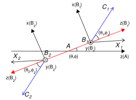
FIG. 1: The definition of the coordinate system in the decay chain $A\to B_{1}B_{2}$ with $B_{1}\to C_{1}X_{1}$ and $B_{2}\to C_{2}X_{2}$. The horizontal arrow represents the flight direction of the mother particle $A$. The red arrows represent the flight directions of $B_{1,2}$ in the rest frame of $A$. The blue arrows represent the flight directions of $C_{1,2}$ in the rest frame of $B_{1,2}$ respectively. $\phi_{+}$ defined in Eq. 1 thus represents the angle between the decay plane of $B_{1}$ and that of $B_{2}$.

According to the helicity formalism developed by Jacob and Wick JacobWick , the amplitude is

$$\mathcal{A} =\sum_{\lambda_{1},\lambda_{2}}F_{\lambda_{1}\lambda_{2}}^{J}D_{M,\lambda_{1}-\lambda_{2}}^{J*}(\Omega)\times G_{\rho_{1}\sigma_{1}}^{j_{1}}D_{\lambda_{1},\rho_{1}-\sigma_{1}}^{j_{1}*}(\Omega_{1})$$ (2)

$$\times G_{\rho_{2}\sigma_{2}}^{j_{2}}D_{\lambda_{2},\rho_{2}-\sigma_{2}}^{j_{2}*}(\Omega_{2})\>.$$

Here the spin of $A$, $B_{1}$ and $B_{2}$ is $J$, $j_{1}$ and $j_{2}$ respectively. $M$ is the third spin-component of $A$. The indices $\lambda_{1,2}$, $\rho_{1,2}$ and $\sigma_{1,2}$ denote the helicity of $B_{1,2}$, $C_{1,2}$ and $X_{1,2}$ respectively. $D_{mn}^{J}(\Omega)\equiv D_{mn}^{J}(\phi,\theta,0)=e^{-im\phi}d_{mn}^{J}(\theta)$ and $D_{mn}^{J}$ ($d_{mn}^{J}$) is the Wigner $D$ ($d$) function. $F_{\lambda_{1}\lambda_{2}}^{J}$ is the helicity amplitude for $A\to B_{1}B_{2}$ and defined as

$$F_{\lambda_{1}\lambda_{2}}^{J}\equiv\langle JM;\lambda_{1},\lambda_{2}|\mathcal{M}|JM\rangle\>,$$ (3)

with $\mathcal{M}$ being the transition matrix derived from the $S$ matrix. It is worthwhile to note that $F_{\lambda_{1}\lambda_{2}}^{J}$ does not rely on $M$ because $\mathcal{M}$ is rotation-invariant. Similarly, $G_{\rho_{i}\sigma_{i}}^{j_{i}}$ is the helicity amplitude for $B_{i}\to C_{i}X_{i}$ ($i=1,2$).

Taking the absolute square of $\mathcal{A}$ and summing over all possible initial and final states, the differential cross section can be written as

$$\frac{d\sigma}{d\Omega d\Omega_{1}d\Omega_{2}}\propto\sum_{M,\lambda_{1},\lambda_{1}^{\prime},\lambda_{2},\lambda_{2}^{\prime}}F_{\lambda_{1}\lambda_{2}}^{J}F_{\lambda_{1}^{\prime}\lambda_{2}^{\prime}}^{J*}e^{i((\lambda_{1}-\lambda_{1}^{\prime})\phi_{1}+(\lambda_{2}-\lambda_{2}^{\prime})\phi_{2})}$$

$$\times d_{M,\lambda_{1}-\lambda_{2}}^{J}(\theta)d_{M,\lambda_{1}^{\prime}-\lambda_{2}^{\prime}}^{J}(\theta)f_{\lambda_{1}\lambda_{1}^{\prime};\lambda_{2}\lambda_{2}^{\prime}}^{j_{1},j_{2}}(\theta_{1},\theta_{2})\>,$$ (4)

with

$$f_{\lambda_{1}\lambda_{1}^{\prime};\lambda_{2}\lambda_{2}^{\prime}}^{j_{1},j_{2}}(\theta_{1},\theta_{2})$$

$$\equiv \sum_{\rho_{1},\sigma_{1},\rho_{2},\sigma_{2}}|G_{\rho_{1}\sigma_{1}}^{j_{1}}|^{2}|G_{\rho_{2}\sigma_{2}}^{j_{2}}|^{2}d_{\lambda_{1},\rho_{1}-\sigma_{1}}^{j_{1}}(\theta_{1})d_{\lambda_{1}^{\prime},\rho_{1}-\sigma_{1}}^{j_{1}}(\theta_{1})$$ (5)

$$\times d_{\lambda_{2},\rho_{2}-\sigma_{2}}^{j_{2}}(\theta_{2})d_{\lambda_{2}^{\prime},\rho_{2}-\sigma_{2}}^{j_{2}}(\theta_{2})\>.$$

Here the summation on $M$ is over the polarization state of $A$ at production. If we do not know the detailed production information, the summation cannot be performed.

Defining $\delta\lambda^{(\prime)}\equiv\lambda_{1}^{(\prime)}-\lambda_{2}^{(\prime)}$, the exponential term in Eq. 4 is equivalent to $e^{i[(\lambda_{1}-\lambda_{1}^{\prime})\phi_{+}-(\delta\lambda-\delta\lambda^{\prime})\phi_{2}]}$. Performing the integration on $\phi_{2}$ and using the definition of $\phi_{+}$, we have (keeping only the terms related with $\phi_{2}$)

$$\int_{0}^{2\pi}d\phi_{2}e^{i((\lambda_{1}-\lambda_{1}^{\prime})\phi_{1}+(\lambda_{2}-\lambda_{2}^{\prime})\phi_{2})}$$

$$= \int_{0}^{\phi_{+}}d\phi_{2}e^{i[(\lambda_{1}-\lambda_{1}^{\prime})\phi_{+}-(\delta\lambda-\delta\lambda^{\prime})\phi_{2}]}$$ (6)

$$+\int_{\phi_{+}}^{2\pi}d\phi_{2}e^{i[(\lambda_{1}-\lambda_{1}^{\prime})(\phi_{+}+2\pi)-(\delta\lambda-\delta\lambda^{\prime})\phi_{2}]}\>.$$

Noting that $(\lambda_{1}-\lambda_{1}^{\prime})$, $\delta\lambda$ and $\delta\lambda^{\prime}$ are integers, the integration gives the requirement $\delta\lambda=\delta\lambda^{\prime}$. Then the differential cross section in terms of $\lambda_{1}^{(\prime)}$, $\delta\lambda^{(\prime)}$ and $\phi_{+}$ is

$$\sum_{\lambda_{1},\lambda_{1}^{\prime},\delta\lambda}F_{\lambda_{1},\lambda_{1}-\delta\lambda}^{J}F_{\lambda_{1}^{\prime},\lambda_{1}^{\prime}-\delta\lambda}^{J*}e^{i(\lambda_{1}-\lambda_{1}^{\prime})\phi_{+}}$$

$$\times\sum_{M}d_{M,\delta\lambda}^{J}(\theta)^{2}f_{\lambda_{1}\lambda_{1}^{\prime};\lambda_{1}-\delta\lambda,\lambda_{1}^{\prime}-\delta\lambda}^{j_{1},j_{2}}(\theta_{1},\theta_{2})\>.$$ (7)

According to the orthogonality relations of the Wigner $D$ functions, we obtain

$$\int d_{mn}^{J}(\theta)^{2}d\cos\theta=\frac{2}{2J+1}\>,$$ (8)

which is independent upon the indices $m,n$. Using this property, we find that integration over $\theta$ of the terms related with $M$ in Eq. 7 only provides a constant factor $\sum_{M}\frac{2}{2J+2}$, which is irrelevant to the normalized angular distributions in the $B_{1,2}$ decays. So we finalize the proof of this theorem in Eq. 9.

$$I(\theta_{1},\theta_{2},\phi_{+})\equiv\frac{1}{\sigma}\frac{d\sigma}{d\cos\theta_{1}d\cos\theta_{2}d\phi_{+}}$$

$$\propto\sum_{\lambda_{1},\lambda_{1}^{\prime},\delta\lambda}F_{\lambda_{1},\lambda_{1}-\delta\lambda}^{J}F_{\lambda_{1}^{\prime},\lambda_{1}^{\prime}-\delta\lambda}^{J*}$$

$$\times e^{i(\lambda_{1}-\lambda_{1}^{\prime})\phi_{+}}f_{\lambda_{1}\lambda_{1}^{\prime};\lambda_{1}-\delta\lambda,\lambda_{1}^{\prime}-\delta\lambda}^{j_{1},j_{2}}(\theta_{1},\theta_{2})\>.$$ (9)

Experimentally, we are interested in the $\phi_{+}$ distribution, which can be used to measure the spin-parity nature of $A$. We integrate out $\theta_{1}$ and $\theta_{2}$ and rewrite $F_{mn}^{J}\equiv R_{mn}^{J}e^{i\varphi_{mn}^{J}}$, where $R_{mn}^{J}$ and $\varphi_{mn}^{J}$ are real. The $\phi_{+}$ distribution turns out to be

$$\frac{d\sigma}{\sigma d\phi_{+}}\propto\sum_{\lambda_{1},\delta\lambda}{R_{\lambda_{1},\lambda_{1}-\delta\lambda}^{J}}^{2}F_{\lambda_{1}\lambda_{1};\lambda_{1}-\delta\lambda,\lambda_{1}-\delta\lambda}^{j_{1},j_{2}}$$

$$+\sum_{\lambda_{1}\neq\lambda_{1}^{\prime}}\sum_{\delta\lambda}R_{\lambda_{1},\lambda_{1}-\delta\lambda}^{J}R_{\lambda_{1}^{\prime},\lambda_{1}^{\prime}-\delta\lambda}^{J}F_{\lambda_{1}\lambda_{1}^{\prime};\lambda_{1}-\delta\lambda,\lambda_{1}^{\prime}-\delta\lambda}^{j_{1},j_{2}}$$

$$\times\cos[(\lambda_{1}-\lambda_{1}^{\prime})\phi_{+}+(\varphi_{\lambda_{1},\lambda_{1}-\delta\lambda}^{J}-\varphi_{\lambda_{1}^{\prime},\lambda_{1}^{\prime}-\delta\lambda}^{J})]\>,\leavevmode\nobreak\$$ (10)

with

$$F_{\lambda_{1}\lambda_{1}^{\prime};\lambda_{2},\lambda_{2}^{\prime}}^{j_{1},j_{2}}\equiv\int f_{\lambda_{1}\lambda_{1}^{\prime};\lambda_{2},\lambda_{2}^{\prime}}^{j_{1},j_{2}}(\theta_{1},\theta_{2})d\cos\theta_{1}d\cos\theta_{2}\>.$$ (11)

Here the second term in Eq. 10 is obtained using the fact that the summation is invariant with the exchange $\lambda_{1}\leftrightarrow\lambda_{1}^{\prime}$.

If the parity is conserved in the decay $A\to B_{1}B_{2}$ (namely, $\mathcal{P}^{-1}\mathcal{M}\mathcal{P}=\mathcal{M}$ with $\mathcal{P}$ being the parity operator), we have

$$R_{mn}^{J}=P_{A}P_{B_{1}}P_{B_{2}}(-1)^{J-j_{1}-j_{2}}R_{-m,-n}^{J}\>,$$

$$\varphi_{mn}^{J}=\varphi_{-m,-n}^{J}\>,$$ (12)

where $P_{A/B_{1}/B_{2}}$ is the parity of $A/B_{1}/B_{2}$ and the factor $-1$ is absorbed in $R_{mn}^{J}$ (namely, we require $0\leq\varphi_{mn}^{J}<\pi$). Noting that the second summation in Eq. 10 is invariant with the index exchange $(\lambda_{1},\lambda_{1}^{\prime},\delta\lambda)\leftrightarrow(-\lambda_{1},-\lambda_{1}^{\prime},-\delta\lambda)$, thus we have

$$\sum_{\lambda_{1}\neq\lambda_{1}^{\prime}}\sum_{\delta\lambda}\cdots=\frac{1}{2}\sum_{\lambda_{1}\neq\lambda_{1}^{\prime}}\sum_{\delta\lambda}\cdots+\frac{1}{2}\sum_{-\lambda_{1}\neq-\lambda_{1}^{\prime}}\sum_{-\delta\lambda}\cdots\>.$$ (13)

Using the symmetry relation in Eq. 12, this summation turns out to be

$$\frac{1}{2}\sum_{\lambda_{1}\neq\lambda_{1}^{\prime}}\sum_{\delta\lambda}R_{\lambda_{1},\lambda_{1}-\delta\lambda}^{J}R_{\lambda_{1}^{\prime},\lambda_{1}^{\prime}-\delta\lambda}^{J}\times\left\{F_{\lambda_{1}\lambda_{1}^{\prime};\lambda_{1}-\delta\lambda,\lambda_{1}^{\prime}-\delta\lambda}^{j_{1},j_{2}}\right.$$

$$\times\cos[(\lambda_{1}-\lambda_{1}^{\prime})\phi_{+}+(\varphi_{\lambda_{1},\lambda_{1}-\delta\lambda}^{J}-\varphi_{\lambda_{1}^{\prime},\lambda_{1}^{\prime}-\delta\lambda}^{J})]$$

$$+F_{-\lambda_{1},-\lambda_{1}^{\prime};-\lambda_{1}+\delta\lambda,-\lambda_{1}^{\prime}+\delta\lambda}^{j_{1},j_{2}}$$

$$\left.\times\cos[(\lambda_{1}-\lambda_{1}^{\prime})\phi_{+}-(\varphi_{\lambda_{1},\lambda_{1}-\delta\lambda}^{J}-\varphi_{\lambda_{1}^{\prime},\lambda_{1}^{\prime}-\delta\lambda}^{J})]\right\}\>.$$ (14)

Focusing on the expressions of Eq. 11 and Eq. 5, we are able to show that

$$F_{\lambda_{1}\lambda_{1}^{\prime};\lambda_{1}-\delta\lambda,\lambda_{1}^{\prime}-\delta\lambda}^{j_{1},j_{2}}=F_{-\lambda_{1},-\lambda_{1}^{\prime};-\lambda_{1}+\delta\lambda,-\lambda_{1}^{\prime}+\delta\lambda}^{j_{1},j_{2}}\>,$$ (15)

using the following property of the Wigner $d$ function

$$d_{mn}^{j}(\pi-\theta)=(-1)^{j-n}d_{-m,n}^{j}(\theta)\>.$$ (16)

With Eq. II and Eq. 15, Eq. 10 can be simplified as

$$\frac{d\sigma}{\sigma d\phi_{+}}\propto\sum_{\lambda_{1},\delta\lambda}{R_{\lambda_{1},\lambda_{1}-\delta\lambda}^{J}}^{2}F_{\lambda_{1}\lambda_{1};\lambda_{1}-\delta\lambda,\lambda_{1}-\delta\lambda}^{j_{1}j_{2}}$$

$$+\sum_{\lambda_{1}\neq\lambda_{1}^{\prime}}\sum_{\delta\lambda}R_{\lambda_{1},\lambda_{1}-\delta\lambda}^{J}R_{\lambda_{1}^{\prime},\lambda_{1}^{\prime}-\delta\lambda}^{J}F_{\lambda_{1}\lambda_{1}^{\prime};\lambda_{1}-\delta\lambda,\lambda_{1}^{\prime}-\delta\lambda}^{j_{1}j_{2}}$$

$$\times\cos(\varphi_{\lambda_{1},\lambda_{1}-\delta\lambda}^{J}-\varphi_{\lambda_{1}^{\prime},\lambda_{1}^{\prime}-\delta\lambda}^{J})\cos[(\lambda_{1}-\lambda_{1}^{\prime})\phi_{+}]\>,\leavevmode\nobreak\$$ (17)

This expression is actually the Fourier series for a $2\pi$-periodic even function. Comparing Eq. 10 and Eq. 17, we can see that the terms which are odd with respective to $\phi_{+}$ are forbidden due to parity conservation in the decay $A\to B_{1}B_{2}$.

Now we consider the special case that $B_{1}$ and $B_{2}$ are identical particles and $B_{1,2}$ decay to the same final state, for example, we will study a doubly charged boson decay $H^{++}\to\tau^{+}\tau^{+}\to\pi^{+}\pi^{+}\bar{\nu}_{\tau}\bar{\nu}_{\tau}$. For identical particles, the state with the spin $J$ and the third component $M$ is

$$|JM;\lambda_{1}\lambda_{2}\rangle_{S}=|JM;\lambda_{1}\lambda_{2}\rangle+(-1)^{J}|JM;\lambda_{2}\lambda_{1}\rangle\>,$$ (18)

which satisfies the spin-statistics relation. Here the normalization factor is omitted. The helicity amplitude $F_{\lambda_{1}\lambda_{2}}^{J}=_{S}\langle JM;\lambda_{1}\lambda_{2}|\mathcal{M}|JM\rangle$ has the symmetry$F_{\lambda_{1}\lambda_{2}}^{J}=(-1)^{J}F_{\lambda_{2}\lambda_{1}}^{J}$. This symmetry relation will further constrain the helicity states, namely, the indices $\lambda_{1}$, $\lambda_{1}^{\prime}$ and $\delta\lambda$ in the summation in Eq. 9, 10 and  17.

III Study of $H^{++}\to\tau^{+}\tau^{+}\to\pi^{+}\pi^{+}\bar{\nu}_{\tau}\bar{\nu}_{\tau}$

Ref. ZpZZ is an example of the application of this theorem. It studies the decay $Z^{\prime}\to ZZ\to l^{+}l^{-}l^{+}l^{-}$, where $B_{1,2}$ are identical bosons. Here we consider the decay chain $H^{++}\to\tau^{+}\tau^{+}\to\pi^{+}\pi^{+}\bar{\nu}_{\tau}\bar{\nu}_{\tau}$. For two spin-$\frac{1}{2}$ identical fermions, we write down all states explicitly. The helicity index $\lambda=+\frac{1}{2}$ ($\frac{-1}{2}$) is denoted by $R$ ($L$).

$$|JM;LL\rangle_{S}= (1+(-1)^{J})|JM;LL\rangle$$ (19)

$$\mathcal{P}|JM;LL\rangle_{S}=-|JM;RR\rangle_{S}$$

$$|JM;RR\rangle_{S}= (1+(-1)^{J})|JM;RR\rangle$$ (20)

$$\mathcal{P}|JM;RR\rangle_{S}=-|JM;LL\rangle_{S}$$

$$|JM;LR\rangle_{S}= |JM;LR\rangle+(-1)^{J}|JM;RL\rangle$$ (21)

$$\mathcal{P}|JM;LR\rangle_{S}=-|JM;LR\rangle_{S}$$

The third state is already a parity eigenstate. The first two states can be combined to have a definite parity.

$$(1+(-1)^{J})(|JM;LL\rangle\pm|JM;RR\rangle)\>,\quad P=\mp 1$$ (22)

In addition, the angular momentum conservation requires $|\lambda_{1}-\lambda_{2}|\leq J$. Now we can give the selection rules, which are summarized in Table 1. We can see that the states with odd spin and even parity are forbidden. For comparison, the selection rules for a neutral particle decaying to spin-$\frac{1}{2}$ fermion anti-fermion pair are summarized in Table 2.

In future electron-electron colliders, $H^{--}$ may be produced in the process $e^{-}e^{-}\to H^{--}$. However, the reaction rate for a spin-1 $H^{--}$ will be highly suppressed because the vector coupling requires that both electrons have the same handness while the only allowed state is $|LR\rangle-|RL\rangle$. Similarly, the production rate for a scalar $H^{--}$ is also highly suppressed. This is called “helicity suppression”.

TABLE 1: Selection rules for a particle decaying to two spin-$\frac{1}{2}$ identical fermions.

Parity	$J=0$	$J=2,4,6,\ldots$	$J=1,3,5,\ldots$
even	$|LL\rangle-|RR\rangle$	$|LL\rangle-|RR\rangle$	forbidden
odd	$|LL\rangle+|RR\rangle$	$|LL\rangle+|RR\rangle$	$|LR\rangle-|RL\rangle$
		$|LR\rangle+|RL\rangle$

TABLE 2: Selection rules for a particle decaying to spin-$\frac{1}{2}$ fermion anti-fermion pair.

Parity	$J=0$	$J=2,4,6,\ldots$	$J=1,3,5,\ldots$
even	$|LL\rangle+|RR\rangle$	$|LL\rangle+|RR\rangle$	$|LL\rangle-|RR\rangle$
		$|LR\rangle+|RL\rangle$	$|LR\rangle-|RL\rangle$
odd	$|LL\rangle-|RR\rangle$	$|LL\rangle-|RR\rangle$	$|LL\rangle+|RR\rangle$
		$|LR\rangle-|RL\rangle$	$|LR\rangle+|RL\rangle$

Replacing $A$, $B_{1,2}$ and $C_{1,2}$ by $H^{++}$, $\tau^{+}$ and $\pi^{+}$ respectively in Eq. 2, the amplitude is

$$\mathcal{A}= G_{0\frac{1}{2}}^{\frac{1}{2}}G_{0\frac{1}{2}}^{\frac{1}{2}}e^{iM\phi}\left[F_{RR}^{J}d_{M0}^{J}(\theta)e^{i(\frac{1}{2}\phi_{1}+\frac{1}{2}\phi_{2})}\sin\frac{\theta_{1}}{2}\sin\frac{\theta_{2}}{2}\right.$$ (23)

$$+\left.F_{LL}^{J}d_{M0}^{J}(\theta)e^{-i(\frac{1}{2}\phi_{1}+\frac{1}{2}\phi_{2})}\cos\frac{\theta_{1}}{2}\cos\frac{\theta_{2}}{2}\right.$$

$$-\left.F_{LR}^{J}d_{M,-1}^{J}(\theta)e^{i(-\frac{1}{2}\phi_{1}+\frac{1}{2}\phi_{2})}\cos\frac{\theta_{1}}{2}\sin\frac{\theta_{2}}{2}\right.$$

$$-\left.F_{RL}^{J}d_{M,1}^{J}(\theta)e^{i(\frac{1}{2}\phi_{1}-\frac{1}{2}\phi_{2})}\sin\frac{\theta_{1}}{2}\cos\frac{\theta_{2}}{2}\right]\>.$$

Here we have only one decay helicity amplitude, $G_{0\frac{1}{2}}^{\frac{1}{2}}$, for the $\tau^{+}$ decay. This is because $\pi^{+}$ is a pseudo-scalar and $\bar{\nu}_{\tau}$ is right-handed. The angular correlation function is

$$I(\theta_{1},\theta_{2},\phi_{+})\propto 1+\cos\theta_{1}\cos\theta_{2}\>,\quad\text{for odd }J$$

$$I(\theta_{1},\theta_{2},\phi_{+})\propto 1+a_{J}^{2}+(1-a_{J}^{2})\cos\theta_{1}\cos\theta_{2}$$ (24)

$$-P_{H}\sin\theta_{1}\sin\theta_{2}\cos\phi_{+}\>,\quad\text{for even }J\quad\quad$$

Here for even $J$, $a_{J}$ is defined as $a_{J}\equiv|F_{LR}^{J}|/|F_{RR}^{J}|$. $P_{H}$ is the parity of $H^{++}$. We can see that the polarization information of $H^{++}$ does not appear in the angular distributions. The $\phi_{+}$ distribution is

$$\frac{d\sigma}{\sigma d\phi_{+}}\propto\left\{\begin{array}[]{ll}1&\text{for odd }J\\ 1-P_{H}\frac{\pi^{2}}{16}\frac{1}{1+a_{J}^{2}}\cos\phi_{+}&\text{for even }J\\ \end{array}\right.\>.$$

The $\phi_{+}$ distributions for different $J^{P}$s are shown in Fig. 2, where $a_{J}=1$ is assumed for illustration.

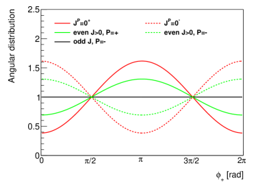
FIG. 2: The $\phi_{+}$ distributions for different $J^{P}$s. The black line represents odd $J$. The red solid (dashed) curve represents $J^{P}=0^{+}(0^{-})$. The green solid (dashed) curve represents even $J>0$ with even (odd) parity assuming $a_{J}=1$.

Here are a few conclusions.

1. The $\phi_{+}$ distribution is uniform for odd $J$.

2. For $J=0$, the helicity amplitudes $F_{LR}^{J}$ and $F_{RL}^{J}$ are forbidden due to angular momentum conservation. Thus $a_{J}=0$ and the $\phi_{+}$ distribution becomes

   $$\frac{d\sigma}{\sigma d\phi_{+}}\propto 1-P_{H}\frac{\pi^{2}}{16}\cos\phi_{+}\>,$$ (25)

   which is the same as that in the decay $h(125)\to\tau^{+}\tau^{-}\to\pi^{+}\pi^{-}\nu_{\tau}\bar{\nu}_{\tau}$.

3. For nonzero even $J$, the $\phi_{+}$ distribution depends upon $J$ through the amplitude ratio $a_{J}$.

Experimentally, it is difficult to reconstruct the $\tau$ lepton information due to the invisible neutrinos MMC ; mtt_xlg . But we are able to obtain the decay plane angle $\phi_{+}$ in some ways (see a most recent review Ref. BBK and references therein). The so-called impact parameter method ImpactParameter is suitable for the decay $\tau^{+}\to\pi^{+}\bar{\nu}_{\tau}$ studied here. It requires that final $\pi^{+}$s have significant impact parameters, which condition can be satisfied at high-energy colliders such as the Large Hadron Collider (LHC).

IV Conclusions

In summary, for a general decay chain $A\to B_{1}B_{2}\to C_{1}C_{2}\ldots$, we have proved that the angular correlation function $I(\theta_{1},\theta_{2},\phi_{+})$ in the decay of the daughter particles $B_{1,2}$ is independent upon the polarization of the mother particle $A$ at production. It guarantees that the spin-parity nature of the mother particle $A$ can be determined by measuring the angular correlation of the two decay planes $B_{i}\to C_{i}\ldots$ ($i=1,2$) without knowing its production details. This theorem has a simple form if the parity is conserved in the decay $A\to B_{1}B_{2}$. Taking a potential doubly-charged particle decay $H^{++}\to\tau^{+}\tau^{+}$ as example, we present the selection rules for various spin-parity combinations. It is found that this decay is forbidden for the $H^{++}$ with odd spin and even parity. Furthermore, we show that the angle between the two $\tau$ decay plans is an effective observable to determine the spin-parity nature of $H^{++}$.

V Acknowledgement

Li-Gang Xia would like to thank Fang Dai for many helpful discussions. The author is also indebted to Yuan-Ning Gao for enlightening discussions. This work is supported by the General Financial Grant from the China Postdoctoral Science Foundation (Grant No. 2015M581062).

References

(1) G. Aad et al., ATLAS Collaboration, Phys. Lett. B 716, 1 (2012).
(2) S. Chatrchyan et al., CMS Collaboration, Phys. Lett. B 716, 30 (2012).
(3) G. Aad et al., ATLAS Collaboration, JHEP 1503, 041 (2015).
(4) G. Aad et al., ATLAS Collaboration, Eur. Phys. J. C, 72, 2244 (2012).
(5) S. Chatrchyan et al., CMS Collaboration, Eur.Phys.J.C, 72, 2189 (2012).
(6) J. R. Dell’Aquila and C. A. Nelson, Phys. Rev. D 33, 80 (1986).
(7) J. R. Dell’Aquila and C. A. Nelson, Phys. Rev. D 33, 93 (1986).
(8) J. R. Dell’Aquila and C. A. Nelson, Phys. Rev. D 33, 101 (1986).
(9) M. R. Buckley, H. Murayama, W. Klemm, and V. Rentala, Phys. Rev. D 78, 014028 (2008).
(10) F. Boudjema and R. K. Singh, JHEP 0907, 028 (2009).
(11) G. Aad et al., ATLAS Collaboration, Eur. Phys. J. C, 75, 476 (2015), Eur. Phys. J. C, 76, 152 (2016).
(12)
G. Aad et al., ATLAS Collaboration, Eur. Phys. J. C, 75, 231 (2015).
(13)
G. Aad et al., ATLAS Collaboration, Phys. Lett. B, 726, 120 (2013).
(14)
V. Khachatryan et al., CMS Collaboration, Phys. Rev. D 92, 012004 (2012).
(15)
S. Chatrchyan et al., CMS Collaboration, Phys. Rev. Lett. 110, 081803 (2013).
(16)
M. Jacob and G.C. Wick, Annals Phys. 281, 774-799 (2000).
(17) W.-Y.
Keung, I. Low, and J. Shu, Phys. Rev. Lett. 101, 091802 (2008).
(18) A. Elagin, P. Murat, A.
Pranko, and A. Safonov, Nucl. Instrum. Meth. A 654, 481 (2011).
(19) Li-Gang Xia, Chin. Phys. C 40, 113003 (2016).
(20) S. Berge, W. Bernreuther, and S. Kirchner, Phys. Rev. D 92, 096012 (2015).
(21) S. Berge and W. Bernreuther, Phys. Lett. B 671, 470 (2009).