GMC Collisions as Triggers of Star Formation. III.
Density and Magnetically Regulated Star Formation

Abstract

We study giant molecular cloud (GMC) collisions and their ability to trigger star cluster formation. We further develop our three dimensional magnetized, turbulent, colliding GMC simulations by implementing star formation sub-grid models. Two such models are explored: (1) “Density-Regulated,” i.e., fixed efficiency per free-fall time above a set density threshold; (2) “Magnetically- Regulated,” i.e., fixed efficiency per free-fall time in regions that are magnetically supercritical. Variations of parameters associated with these models are also explored. In the non-colliding simulations, the overall level of star formation is sensitive to model parameter choices that relate to effective density thresholds. In the GMC collision simulations, the final star formation rates and efficiencies are relatively independent of these parameters. Between non-colliding and colliding cases, we compare the morphologies of the resulting star clusters, properties of star-forming gas, time evolution of the star formation rate (SFR), spatial clustering of the stars, and resulting kinematics of the stars in comparison to the natal gas. We find that typical collisions, by creating larger amounts of dense gas, trigger earlier and enhanced star formation, resulting in 10 times higher SFRs and efficiencies. The star clusters formed from GMC collisions show greater spatial sub-structure and more disturbed kinematics.

1 Introduction

Most stars are thought to form in clusters within giant molecular clouds (GMCs). GMCs have typical hydrogen number densities of $n_{\rm H}=100\>{\rm cm^{-3}}$, diameters of $\sim$tens of parsecs, masses of up to $10^{6}\>M_{\odot}$, and average temperatures of $\sim 10-30\>{\rm K}$. Dense clumps within GMCs, potentially traced as, e.g., Infrared Dark Clouds (IRDCs), are recognized as being the likely precursors to star clusters (e.g. Rathborne et al., 2006; Tan et al., 2014; Butler & Tan, 2009, 2012). IRDCs have such high mass surface densities ($\Sigma\gtrsim 0.1~{}{\rm g\>cm^{-2}}$) that they are dark at mid-IR ($\sim 10~{}{\rm\mu m}$) and even far-IR ($\sim 70~{}{\rm\mu m}$) (e.g., Lim & Tan, 2014). Their low temperatures ($10-20$K) (see, e.g., Pillai et al., 2006; Wang et al., 2008; Sakai et al., 2008; Chira et al., 2013), high volume densities ($n_{\rm H}>10^{5}~{}{\rm cm^{-3}}$), relatively compact sizes ($\sim$few pc), and masses ($\sim 10^{2}-10^{5}~{}M_{\odot}$) indicate that they have the potential to be the precursors to most of the observed mass range of star clusters known in the Galaxy. The initial and early stages of star cluster formation can also be traced by dust continuum emission (e.g., Ginsburg et al., 2012) and by samples based on emission of dense gas tracers (e.g., Ma et al., 2013). Surveys of young embedded stars also can probe the structure (e.g., Jaehnig et al., 2015), age distribution (e.g., Da Rio et al., 2014) and kinematics of young clusters (e.g., Foster et al., 2015; Cottaar et al., 2015).

Currently, the dominant processes that induce the collapse and fragmentation of GMCs into star-forming clumps are poorly understood. Various theoretical models include regulation by turbulence (e.g., Krumholz & McKee, 2005), regulation by magnetic fields (e.g., Van Loo et al., 2015), triggering by stellar feedback (e.g., supernova; Inutsuka et al., 2015), triggering by converging atomic flows (e.g., Heitsch et al., 2009), and triggering via converging molecular flows, i.e., GMC-GMC collisions (e.g., Scoville et al., 1986; Tan, 2000).

Semi-analytic models (Tan, 2000) and numerical simulations (Tasker & Tan, 2009; Fujimoto et al., 2014; Dobbs et al., 2015) of global galactic disks have shown that GMCs collide relatively frequently due to the approximately 2D geometry of a thin disk and interaction rates driven by differential rotation of galactic orbits. The average timescale between GMC collisions was found to be about 20% of a local orbital period within a flat rotation curve disk (Tasker & Tan, 2009) (see also Fujimoto et al., 2014; Dobbs et al., 2015). A growing number of numerical studies have also shown that collisions between molecular clouds can provide conditions favorable for massive star and star cluster formation (see e.g., Habe & Ohta, 1992; Klein & Woods, 1998; Anathpindika, 2009; Takahira et al., 2014; Haworth et al., 2015a, b; Balfour et al., 2015). We note that in general comparison of the results between the simulations of different groups is complicated by the use of different initial conditions, different numerical methods and different included physics.

Our approach here is to systematically build-up realism for our GMC collision simulations by including additional physics step by step that allows an understanding of the relative importance of different input assumptions. Wu et al. (2015, hereafter Paper I) and Wu et al. (2017, hereafter Paper II) developed a numerical study of GMC-GMC collisions, focusing on understanding the physical mechanisms as well as using them to predict observational diagnostics. Comparing magnetized, supersonically turbulent GMCs in colliding and non-colliding cases over a wide parameter space and investigating a varied array of potential observational signatures, they found that a number of indicators suggest similarities between the colliding scenarios to observed GMCs and IRDCs. Further, dynamical virial analysis suggested that dense ¹³CO-defined structures created through GMC collisions were more likely to collapse and form massive star clusters when compared with more quiescently evolving structures.

The next stage in our work is the crucial transition from collapsing clumps into star clusters. Properties of the stars that form, along with their dynamical evolution shortly thereafter, may provide insight into the dominant star formation mechanisms. The goal of this study is to answer the question: do realistic models of GMC collisions create star clusters that closely match the properties of observed young star-forming regions? We approach this question by further building upon our previous numerical framework of GMCs through the development of star formation sub-grid models, one of which is a novel magnetically-regulated model. We combine our existing gas-focused observational diagnostic methods with additional information from the population of star particles. Thus, we hope to provide insight to the star formation process by analyzing the evolution of IRDC-type structures into young star clusters.

Section 2 describes our numerical setup and the various star formation models. We then present our results in Section 3, which include: gas and star cluster morphologies (§3.1), properties of star-forming gas (§3.2), global star formation rates (SFRs) and efficiencies (§3.3), spatial clustering (§3.4), and star particle kinematics (§3.5). In Section 4 we discuss our conclusions.

2 Numerical Model

2.1 Initial Conditions

We further develop the numerical framework described in Paper II and introduce two star formation routines. Our GMCs are identical to those initialized in Paper II, which are motivated by observed GMC properties. The clouds are self-gravitating, supersonically turbulent, and magnetized. They are initialized with identical densities and offset by an impact parameter. The clouds are embedded in an ambient medium of ten times lower density (i.e., an atomic cold neutral medium, CNM), which for the colliding case, is converging along with the GMCs. The initial simulation properties are summarized in Table 1.

The simulation domain is $(128\>{\rm pc})^{3}$ and contains two neighboring GMCs. The GMCs are initially uniform spheres, with Hydrogen number densities of $n_{\rm H,GMC}=100\>{\rm cm^{-3}}$ and radii $R_{\rm GMC}=20.0$ pc. This gives each GMC a mass $M_{\rm GMC}=9.3\times 10^{4}\>M_{\odot}$. The ambient gas represents the atomic cold neutral medium (CNM) and has a density of $n_{\rm H,0}=10\>{\rm cm^{-3}}$. The centers of the GMCs are offset by $2R_{\rm GMC}$ in the collision axis ($x$), 0 in the $y$-axis, and $b=0.5R_{\rm GMC}$ in the $z$-axis.

To approximate the density and velocity structures observed in GMCs, our clouds are initialized with a supersonic turbulent velocity field which is random, purely solenoidal, and follows the $v_{k}^{2}\propto k^{-4}$ relation, where $k=\pi/d$ is the wavenumber for an eddy diameter $d$. Conventionally, the “$k$-mode” is normalized to the simulation box length. The gas within the GMC is initialized with Mach number $\mathcal{M}_{s}\equiv\sigma/c_{s}=23$ (for $T=15$ K conditions), of order virial. We set our fiducial $k$-modes to be $\left\{2,...,20\right\}$, where each mode within this range is excited. This is representative of the large-scale turbulent velocities (small $k$) spanning from the GMC diameters down to a small enough minimum scale (large $k$), which is numerically resolved, but expected to cascade to smaller scales. We do not drive turbulence, instead letting it decay within a few dynamical times. Note also that turbulence is initialized only within the initial volume of the GMCs while we leave the ambient medium non-turbulent. Note also the GMC collision will also drive turbulence in the clouds in that case.

A large-scale uniform magnetic field of strength $10\>{\rm\mu G}$ is initialized throughout the box at an angle $\theta=60^{\circ}$ with respect to the collision ($x$-) axis. This choice of $|\bm{B}|$ is motivated by the Zeeman measurements of typical GMC field strengths, summarized by Crutcher (2012).

In the fiducial colliding case, the bulk flows (including both the ambient gas and the GMCs) have a relative velocity of $v_{\rm rel}=10\>{\rm km\>s^{-1}}$. In the non-colliding case, there is no bulk velocity flow.

The simulations are run for $5\>{\rm Myr}$ to investigate the onset of star formation. Note that this is $1\>{\rm Myr}$ longer than the simulations described in Paper II, which focused on gas properties of the pre-star-forming clump. Note also that the freefall time given the initial uniform density GMCs is $t_{\rm ff}=(3\pi/[32G\rho])^{1/2}\simeq 4.35$ Myr. However, the values of $t_{\rm ff}$ for the denser substructures created by turbulence and by the collision are much shorter. Star formation is expected to occur in both non-colliding and colliding cases, with the detailed properties of resulting star clusters acting as the key point of our investigation.

Table 1: Initial Simulation Properties

				GMC		Ambient
$n_{\rm H}$		(${\rm cm}^{-3}$)		100		10
$R$		(${\rm pc}$)		20		…
$M$		($M_{\odot}$)		$9.3\times 10^{4}$		…
$T$		(K)		15		150
$t_{\rm ff}$		(Myr)		4.35		…
$c_{\rm s}$		(km/s)		0.23		0.72
$v_{A}$		(km/s)		1.84		5.83
$v_{\rm vir}$		(km/s)		4.9		…
$\sigma$		(km/s)		5.2		…
$\mathcal{M}_{\rm s}$		…		23		…
$\mathcal{M}_{A}$		…		2.82		…
$k$-mode		($k_{1},k_{2}$)		(2,20)		…
$v_{\rm bulk}$		(km/s)		$\pm 5$		$\pm 5$
$B$		(${\rm\mu G}$)		10		10
$\lambda$		…		4.3		1.5
$\beta$		…		0.015		0.015

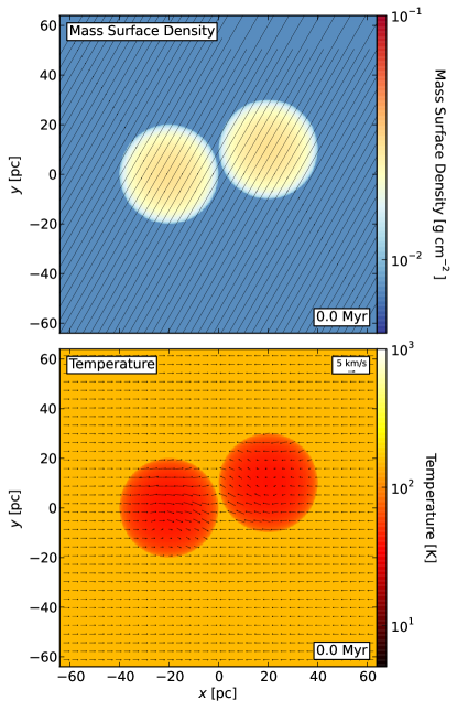
Figure 1: Initial conditions. Top panel: Mass surface density, shown together with magnetic field structure (gray lines). Bottom panel: Mass-weighted temperature, shown together with the velocity field (black vectors). The colliding case is shown. GMCs 1 (left) and 2 (right) have identical dimensions with an initial separation of their centers of $2R_{\rm GMC}$ in the x-direction and 0 in the z-direction. In the y-direction, they are offset by an impact parameter $b=0.5R_{\rm GMC}$.

2.2 Numerical Code

Our models are run using Enzo, a magnetohydrodynamics (MHD) adaptive mesh refinement (AMR) code (Bryan et al., 2014). We use the Dedner-MHD method, which solves the solves the MHD equations using the Harten-Lax-van Leer with Discontinuities (HLLD) method and a piecewise linear reconstruction method (PLM). The time is evolved using the MUSCL 2nd-order Runge-Kutta method. The $\nabla\cdot\bf{B}=0$ solenoidal constraint of the magnetic field is maintained via a hyperbolic divergence cleaning method (Dedner et al., 2002; Wang & Abel, 2008).

The simulation domain is realized with a top level root grid of $128^{3}$ with 3 additional levels of AMR. Our models thus have an effective resolution of $1024^{3}$, with a minimum grid cell size of 0.125 pc. We refine solely on the local Jeans length, setting a necessary requirement of resolving by 8 cells, i.e., higher than the 4 cells typically used to avoid artificial fragmentation (Truelove et al., 1997)). Our higher resolution leads to larger volumes of the GMCs being better resolved and thus generally better resolution of, e.g., shocks (see also Few et al., 2016). We note that the Jeans criterion assumes purely thermal support. The gas in our simulations also has some magnetic support, so its effective “magneto-Jeans length” will be significantly larger than the thermal Jeans length in directions perpendicular to the magnetic field.

Due to the relatively high bulk velocities and potentially strong magnetic fields, we require the use of the “dual energy formalism” (Bryan et al., 2014) , which separately solves the internal energy equation as well as the total energy equation, ensuring accurate calculation of pressures and temperatures in these conditions. If the ratio of thermal to total energy is less than 0.001, then the temperature is calculated from the internal pressure. Otherwise, the total energy is used.

Additionally, we employ the “Alfvén limiter” (described in Paper II) to avoid exceedingly small timesteps set by Alfvén waves. This acts by choosing a maximum Alfvén velocity, $v_{A,{\rm max}}=B/\sqrt{4\pi\rho_{\rm min}}=1\times 10^{7}\>{\rm cm\>s^{-1}}$, and setting a density floor that is determined by the magnetic field. This predominantly affects only small pockets of very low-density gas with which we are less interested, and thus the dynamical results are deemed unaffected by this limiter.

2.3 Thermal Processes

We assume a constant mean particle mass ($\mu=2.33\>m_{\rm H}$) throughout the simulation domain for simplicity, as our focus is on the dense molecular gas of GMCs. We also choose a constant adiabatic index $\gamma=5/3$. Note that this essentially ignores certain excitation modes of $\rm H_{2}$ that may be relevant (i.e., shocks), but it is still the most appropriate single-valued choice of $\gamma$, given our focus on the dynamics of cold $\rm H_{2}$. Also, we assume $n_{\rm He}=0.1n_{\rm H}$, giving a mass per H of $2.34\times 10^{-24}\>{\rm g}$.

The PDR-based heating and cooling functions developed in Paper I are again used in these simulations. The assumptions are: (1) FUV radiation field of $G_{0}=4$ (i.e., appropriate conditions for the inner Galaxy, e.g., at Galactocentric distances of $\sim 4$ kpc) and (2) a background cosmic ray ionization rate of $\zeta=1.0\times 10^{-16}\>{\rm s^{-1}}$. The heating/cooling functions trace the atomic to molecular transition and recreate a multi-phase ISM. They span density and temperature ranges of $10^{-3}\leq n_{\rm H}/{\rm cm^{-3}}\leq 10^{6}$ (extended to $10^{1}0~{}{\rm cm^{-3}}$ via extrapolation) and $2.7\leq T/{\rm K}\leq 10^{7}$, respectively.

We use the Grackle external chemistry and cooling library (Smith et al., 2016) to incorporate our heating/cooling functions in tabular form into Enzo, modifying the energy equation.

In order to avoid numerical instabilities related to the heating/cooling processes, we limit the timestep on each AMR level to a factor of 0.2 the minimum cooling time. Additionally, we set a hard floor for the minimum cooling timestep of $625~{}{\rm yrs}$.

Table 2: Simulation Runs with Star Formation Sub-Grid Models

Name	Star Formation	$v_{\rm rel}$	Cell Size	$n_{\rm H,sf}$	$t_{\rm ff}$	$m_{\rm gas,min}$	$m_{\rm\star,min}$	$c_{1}$
	Model	(${\rm km\>s^{-1}}$)	(pc)	(cm-3)	(yr)	($M_{\odot}$)	($M_{\odot}$)
d-0.5-nocol	dens. reg.	0	0.125	$0.5\times 10^{6}$	$6.2\times 10^{4}$	32	10	-
d-1-nocol	dens. reg.	0	0.125	$1.0\times 10^{6}$	$4.4\times 10^{4}$	63	10	-
d-2-nocol	dens. reg.	0	0.125	$2.0\times 10^{6}$	$3.1\times 10^{4}$	126	10	-
B-0.5-nocol	mag. reg.	0	0.125	$3.55\times 10^{5}$	$7.3\times 10^{4}$	20	10	0.063
B-1-nocol	mag. reg.	0	0.125	$3.55\times 10^{5}$	$7.3\times 10^{4}$	20	10	0.126
B-2-nocol	mag. reg.	0	0.125	$3.55\times 10^{5}$	$7.3\times 10^{4}$	20	10	0.252
B-1-1M-nocol	mag. reg.	0	0.125	$3.55\times 10^{4}$	$2.3\times 10^{5}$	2	1	0.126
d-0.5-col	dens. reg.	10	0.125	$0.5\times 10^{6}$	$6.2\times 10^{4}$	32	10	-
d-1-col	dens. reg.	10	0.125	$1.0\times 10^{6}$	$4.4\times 10^{4}$	63	10	-
d-2-col	dens. reg.	10	0.125	$2.0\times 10^{6}$	$3.1\times 10^{4}$	126	10	-
B-0.5-col	mag. reg.	10	0.125	$3.55\times 10^{5}$	$7.3\times 10^{4}$	20	10	0.063
B-1-col	mag. reg.	10	0.125	$3.55\times 10^{5}$	$7.3\times 10^{4}$	20	10	0.126
B-2-col	mag. reg.	10	0.125	$3.55\times 10^{5}$	$7.3\times 10^{4}$	20	10	0.252
B-1-1M-col	mag. reg.	10	0.125	$3.55\times 10^{4}$	$2.3\times 10^{5}$	2	1	0.126

2.4 Star Formation

We utilize the particle machinery of Enzo to model star formation. Specifically, star particles (i.e., collisionless, point particles with mass $m_{\star}$) form within a simulation cell if certain local criteria are met. Two star formation routines are developed: (1) density-regulated star formation; (2) magnetically-regulated star formation.

2.4.1 Density-regulated star formation

Our first star formation routine is a “density-regulated” model, based on that of Van Loo et al. (2013) (see also Butler et al., 2015). Stars are formed within a cell only if they have been refined to the finest level of resolution and the density exceeds a particular threshold value, $n_{\rm H,sf}$. The fiducial star formation density threshold is chosen to be $n_{\rm H,sf}=10^{6}~{}{\rm cm^{-3}}$, which is set partly based on observed densities of pre-stellar cores (e.g., Kong et al., 2017). We will consider variation of this parameter by a factor of two to higher and lower values. The temperature in the cell is also required to be $<3000$ K, to avoid star formation in dense, shock-heated regions, but we will see that this constraint is not of practical concern for the simulations presented here. Note that there is no requirement for gravitational boundedness of gas in the cell. Nor is there a requirement for net convergence of gas flow to the cell. These choices are motivated by the fact such conditions are not well resolved on the local scales associated with an individual cell. In addition, we expect that processes such as turbulence and diffusion of magnetic flux that are occurring on sub-grid scales (or scales near the grid scale that are not well resolved) will regulate star formation, e.g., creating local conditions that are gravitationally unstable, perhaps via converging flows. With these points in mind, this star formation sub-grid model using a density threshold is thus designed to be as simple as possible, enabling us to gain a clear understanding of how the results depend on its input parameters.

In cells meeting the above conditions, star particles are then produced so that the SFR is, on average, equal to that expected if there is a fixed star formation efficiency per local free-fall time, $\epsilon_{\rm ff}$, where the local free-fall time, $t_{\rm ff}$, is expressed as

$$t_{\rm ff} = \left(\frac{3\pi}{32G\rho}\right)^{1/2}$$ (1)

$$= 4.4\times 10^{4}n_{\rm H,6}^{-1/2}\>{\rm yr},$$ (2)

i.e., the value for collapse of a uniform density sphere, where $n_{\rm H,6}\equiv n_{\rm H}/10^{6}\>{\rm cm^{-3}}$. We adopt a fiducial choice of $\epsilon_{\rm ff}=0.02$, motivated by observations of GMCs, their star-forming clumps and stellar populations in embedded clusters, which suggest fairly low and density-independent values of $\epsilon_{\rm ff}$ (see, e.g., Zuckerman & Evans, 1974; Krumholz & Tan, 2007; Da Rio et al., 2014). Thus the SFR is

$$\dot{m}_{\star} = \epsilon_{\rm ff}\frac{m_{\rm gas}}{t_{\rm ff}}$$ (3)

$$= 2.9\times 10^{-5}\left(\frac{\epsilon_{\rm ff}}{0.02}\right)\left(\frac{\Delta x}{0.125\>{\rm pc}}\right)^{3}n_{\rm H,6}^{3/2}\>M_{\odot}\>{\rm yr}^{-1},$$ (4)

where we have normalized to the minimum cell size, $\Delta x$, relevant for the simulations in this paper.

The timesteps in the simulation are typically quite short, i.e., much less than the signal crossing time of a cell, i.e., $\ll 1.2\times 10^{5}\>$yr for a signal speed of 1 $\rm km\>s^{-1}$. Thus the average mass of stars that are expected to be created in a given cell in a given simulation timestep is often very small, i.e., $<1\>M_{\odot}$.

To enable both a practical computation that does not involve too many star particles, but also with the eventual aim of producing star particles with masses that are characteristic of observed stellar masses, the star formation sub-grid model also involves a parameter of a minimum star particle mass, $m_{\rm\star,min}$. For the density-regulated models we consider here, we set $m_{\rm\star,min}=10\>M_{\odot}$. Thus in this case the star particles represent small (sub-)clusters of stars, since the mean stellar mass is $\lesssim 1\>M_{\odot}$ for realistic stellar initial mass functions (e.g., Parravano et al., 2011) (see also discussion of star particle dynamics in §2.4.3). With this value of $m_{\rm\star,min}$ we are almost always in a regime in which the mass of stars to be created in a given timestep is smaller than $m_{\rm\star,min}$ and so the decision to form a star particle or not needs to be implemented probabilistically, i.e., the “stochastic star formation” regime. In this case, the star particle is formed with probability $\dot{m}_{\star}\Delta t/m_{\rm\star,min}$, where $\Delta t$ is the simulation timestep. If on the other hand $\dot{m}_{\star}\Delta t>m_{\rm\star,min}$ (which can occur in certain circumstances), then the star particle is simply created with this mass.

Another factor affecting the choice of $m_{\rm\star,min}$ is the desire not to change the gas mass in a cell by too large a fraction when the star particle is created, i.e., to avoid too large changes in density, pressure, etc. In general we set an upper limit of this fraction of 0.5. In the fiducial case a cell of size 0.125 pc at the star formation threshold density contains a minimum gas mass of $m_{\rm gas,min}=63\>M_{\odot}$, so this fraction is $\lesssim 0.17$ for these models ($\lesssim 0.34$ for the lower threshold density case).

Overall there are three density (“d”)-regulated runs (i.e., three choices of threshold density) for each of the noncolliding (“nocol”) and colliding (“col”) simulation set-ups. The parameters of these star formation models and simulations are listed in Table 2.

2.4.2 Magnetically-regulated star formation

We introduce a new “magnetically-regulated” star formation model that takes into account magnetic criticality, i.e., star formation is only allowed to proceed if a cell has a mass to flux ratio that is greater than a certain value. If the cell is magnetically “supercritical” by this criterion, then it forms stars at a fixed efficiency per local free-fall time, $\epsilon_{\rm ff}$, where we will adopt the same value of 0.02 that was used in the density-regulated models. Thus this magnetic criticality condition acts to replace the density-threshold criterion of §2.4.1. However, as we discuss below, the choice of $m_{\rm\star,min}$ also introduces an effective minimum density for star formation in this model also.

To assess the mass-to-flux ratio criterion, as an approximation, we treat each grid cell individually and calculate the dimensionless mass-to-flux ratio

$$\mu_{\rm cell}=\frac{\rho\Delta x\sqrt{G}}{Bc_{1}},$$ (5)

where $\rho$ is the density within a cell of length $\Delta x$, $G$ is the gravitational constant, $B$ is the strength of the magnetic field within the cell, and $c_{1}$ comes from defining the critical mass-to-flux ratio as

$$\left(\frac{M}{\Phi}\right)_{\rm crit}=\frac{c_{1}}{\sqrt{G}}$$ (6)

and is ultimately dependent of the geometry of the system. For an infinite disk, the value is $c_{1}=1/(2\pi)$ (Nakano & Nakamura, 1978); for an isolated cloud it is roughly $1/\sqrt{63}\sim 0.126$ (Mouschovias & Spitzer, 1976). We will consider variations of $c_{1}$ of a factor of two to higher and lower values. These and other parameters of the magnetically (“B”)-regulated star formation models are also listed in Table 2. We note that although the true mass-to-flux ratio depends on the geometry of the entire flux tube and cannot be completely confined to a localized quantity, this only acts as a first-order correction.

If a cell is magnetically subcritical (i.e., $\mu_{\rm cell}<1$), the magnetic pressure is deemed strong enough to withstand gravitational contraction, preventing any stars from forming within that cell. For those cells that are magnetically supercritical (i.e., $\mu_{\rm cell}>1$), then star formation may be allowed to occur. However the two other criteria introduced in §2.4.1, i.e., the cell is resolved at the finest refinement level and $T<3000$ K, also must be satisfied. In addition, we also limit the fraction of gas mass in a cell that is turned into stars at a single timestep to be $<0.5$. Given the minimum star particle mass, $m_{\rm\star,min}$, this imposes an “effective density threshold” for the magnetically-regulated star formation model. For this reason, we will investigate magnetically-regulated models with $m_{\rm\star,min}=10\>M_{\odot}$ (as in the density-regulated models), but also with $m_{\rm\star,min}=1\>M_{\odot}$. These choices correspond to effective minimum threshold densities of $n_{\rm H,sf}=3.55\times 10^{5}\>{\rm cm^{-3}}$ for $m_{\star,{\rm min}}=10\>M_{\odot}$ and $n_{\rm H,sf}=3.55\times 10^{4}\>{\rm cm^{-3}}$ for $m_{\star,{\rm min}}=1\>M_{\odot}$.

If all the above conditions are satisfied, then the star formation process is allowed to occur at fixed efficiency per local free-fall time, as described in §2.4.1. We will see that the magnetically-regulated models with $m_{\star,{\rm min}}=1\>M_{\odot}$ can form significant numbers of star particles out of the stochastic regime, but these masses should not be interpreted as being a realistic assessment of the stellar initial mass function, since their values depend on the size of the simulation timestep.

Overall there are four magnetically (“B”)-regulated runs (i.e., three choices of mass-to-flux threshold for $m_{\star,{\rm min}}=10\>M_{\odot}$ and one run with $m_{\star,{\rm min}}=1\>M_{\odot}$ at the fiducial mass-to-flux threshold) for each of the noncolliding (“nocol”) and colliding (“col”) simulation set-ups. The parameters of these star formation models and simulations are also listed in Table 2.

2.4.3 Star particle and star cluster dynamics

Once the star formation criteria are met, mass is removed from the cell and placed into a point-like star particle. These evolve as a collisionless N-body system. However, these are not treated as accreting sink particles, so they do not gain additional mass from the gas, which we expect to be realistic due to the action of stellar winds from the young stars. The particles still interact with the gas gravitationally via a cloud-in-cell (CIC) algorithm which maps the particle positions onto the grid. This limits the closest distances between star particles to the grid resolution, ultimately resulting in softer mutual gravitational interactions. As a result, small scale, i.e., internal, star cluster dynamics is not expected to be well-modeled. However, the early stages and larger scales of the spatial and kinematic distribution of the stars, should be more accurately followed.

Note also that our ability to follow the true internal dynamics of the formed star clusters is limited by the fact that we do not fully allow for the presence of a range of stellar masses, including both low-mass and high-mass stars, or the presence of binary or higher order multiple star systems. However, since our ability to accurately follow the dynamical evolution of the star cluster is mostly limited by the fact that gravitational forces are not well resolved below the grid scale of the simulation, our focus is mostly on the global distribution of stars in the simulations and the large scale spatial and kinematic distributions of the stars in the clusters, e.g., low order spatial mode asymmetries.

The current modeling also does not include feedback from the formed star particles. A goal of a future paper is to include protostellar outflow momentum feedback in these models, but at the moment the star formation that results should be considered a baseline estimate in the limit of zero feedback.

3 Results

We perform analysis of each the simulations, comparing and contrasting star formation models as well as non-colliding vs. colliding cases. In particular, we discuss: morphology of the clouds and clusters (§3.1); properties of star-forming gas (§3.2); global star formation rates (§3.3); spatial clustering of stars (§3.4); and star vs. gas kinematics (§3.5).

3.1 Cloud and Cluster Morphologies

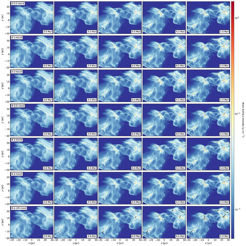
Figure 2: Time evolution of mass surface density, viewed along the $z$-axis, for all non-colliding cases with star formation. The top three rows display the density-regulated SF runs, while the bottom four rows display the magnetically-regulated SF runs, with labels given in the left column. Snapshots at 3.0, 3.5, 4.0, 4.5, and 5.0 Myr (left to right) are shown. Star particles are overplotted as black points.

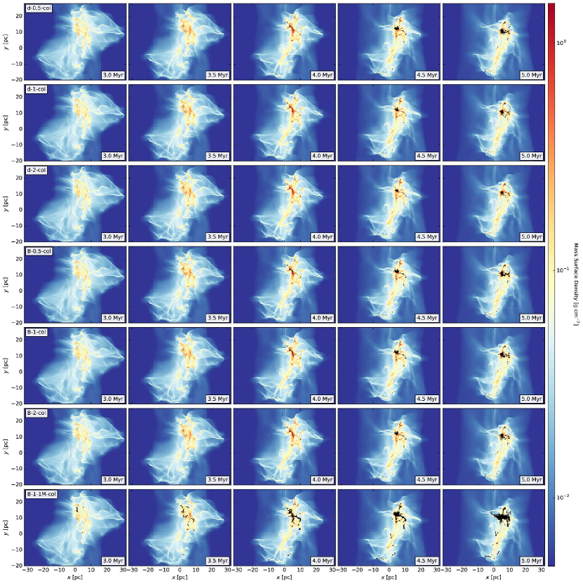
Figure 3: Time evolution of mass surface density, viewed along the $z$-axis, i.e., perpendicular to the collision axis, for all colliding cases with star formation. The top three rows display the density-regulated SF runs, while the bottom four rows display the magnetically-regulated SF runs, with labels given in the left column. Snapshots at 3.0, 3.5, 4.0, 4.5, and 5.0 Myr are shown (left to right). Star particles are overplotted as black points.

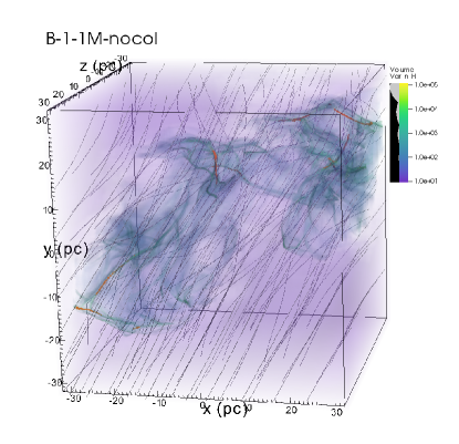
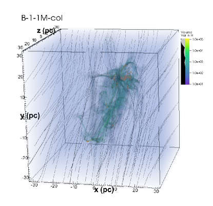
Figure 4: 3D volume rendering of gas density shown together with magnetic field structure (streamlines) and star particles (orange points). Outputs at $t=5.0~{}{\rm Myr}$ are shown for the non-colliding (left) and colliding (right) models using the $m_{\rm\star,min}=1\>M_{\odot}$ magnetically regulated star formation routine. The transfer function is shown along with $n_{\rm H}$.

The morphology of the gas and the stars are shown in Figure 2 for the non-colliding clouds and Figure 3 for the colliding clouds. In the non-colliding cases, the gas evolution is essentially identical, where turbulent velocities and self-gravity create a network of relatively slowly growing filaments with increasing differentiation in mass surface density. Evolution is relatively passive and quiescent. In general, the onset of star formation takes place near $4.5\>{\rm Myr}$ for the $m_{\star,{\rm min}}=10~{}M_{\odot}$ cases and $3.5\>{\rm Myr}$ for the $m_{\star,{\rm min}}=1~{}M_{\odot}$ case.

Both density-regulated and magnetically-regulated models result in pockets of localized star formation concentrated at density peaks within filamentary structures. The slightly more populated network of filaments in the northeast region forms a higher number of (small) star clusters, but overall, star formation is scattered sparsely throughout both GMCs and remains relatively spatially isolated. The magnetically-regulated models form clusters with a higher degree of elongation, i.e., following the axes of the natal filaments. There is also slightly more widespread star formation activity compared with the density regulated case. By $t=5.0~{}{\rm Myr}$, approximately 5-8 clusters have formed in the density-regulated cases, with the higher critical density models forming fewer clusters, whereas 10-12 separate clusters have formed in the magnetically-regulated cases.

Differences are more pronounced in the $m_{\star,{\rm min}}=1~{}M_{\odot}$ case, as stars form in elongated clusters along the filaments instead of the more localized spherical clusters as in the density regulated case or the slightly eccentric clusters as in the $m_{\star,{\rm min}}=10~{}M_{\odot}$ magnetically regulated cases.

However, one needs to bear in mind that the magnetically-regulated models also involve an effective minimum density threshold as an additional requirement for star formation. This threshold density depends on the minimum star particle mass that is allowed in the model via the requirement that no more than 50% of the cell’s gas mass can be converted to a star particle (see §2.4.2). These effective threshold densities are $n_{\rm H,\star min}=3.55\times 10^{5}\>{\rm cm^{-3}}$ for $m_{\star,{\rm min}}=10~{}M_{\odot}$ and $n_{\rm H,\star min}=3.55\times 10^{4}\>{\rm cm^{-3}}$ for $m_{\star,{\rm min}}=1~{}M_{\odot}$. Thus the variation in $m_{\star,{\rm min}}$ is a way of investigating how varying this effective density threshold influences the resulting stellar population. Recall that for star-forming gas, the star formation activity in lower density regions is suppressed because the rate scales inversely with the local free-fall time, i.e., SFR $=\epsilon_{\rm ff}m_{\rm cell}/t_{\rm ff}\propto n_{\rm H}^{3/2}$. Thus the overall SFR in these magnetically-regulated models will depend on both the probability distribution function (PDF) of densities of the gas above the effective threshold density that achieves the magnetic criticality condition. In the simple density-regulated models, the SFR will simply depend on the PDF of densities above the threshold density.

Considering now the GMC collision cases (Figure 3), we see that they produce a much more active and dynamic environment that leads to creation of much denser gas structures (see also Paper II). At the interface of the colliding flows, a primary high-density filamentary structure is formed. This relatively compact, sheet-like structure lies predominantly in the plane perpendicular to the collision axis, with smaller filaments extending outward in various directions. Mass surface densities of $\sim 1~{}{\rm g\>cm^{-3}}$ are reached much sooner compared to the non-colliding case. This results in earlier and more rapid star formation, generally beginning near $3.0$ to $3.5\>{\rm Myr}$ for the $m_{\star,{\rm min}}=10~{}M_{\odot}$ cases and earlier than $3.0\>{\rm Myr}$ for the $m_{\star,{\rm min}}=1~{}M_{\odot}$ case of magnetically-regulated star formation.

In all such cases, the clusters form in the central colliding region, at the peaks of filaments located in the primary filamentary network. These sites often correspond with overdense clumps located at filament junctions, potentially pointing toward star formation triggered by filament-filament interactions on the smaller scale. By $t=4.5~{}{\rm Myr}$, the individual star clusters have grown and merged into one dominant star cluster located near $(x,y)=(5{\rm~{}pc},10{\rm~{}pc})$, while stars continue to form from dense clumps scattered throughout the post-shock colliding region. This large cluster appears to contain multiple populations of smaller star clusters that have merged together through a combination of gravitational attraction and initial velocity inherited from the natal gas of the collision. The spatially separated clusters from earlier times have grown in population and are moving toward the main cluster, while a few smaller clusters are continuing to form along the still-colliding dense filamentary gas. By $t=5.0$ Myr, the main cluster (which has grown to a few thousand stars in the $m_{\star,{\rm min}}=10~{}M_{\odot}$ case and a factor of 10 higher in the $1~{}M_{\odot}$ case) is co-located with the majority of the dense gas, as more star clusters form in the vicinity. There exists a small population of individual stars that form in relative isolation and/or are dynamically ejected from the denser regions.

The factor of two variations in $n_{\rm H,sf}$ do not greatly alter the overall cluster morphology. However, there are small differences in total cluster number as well as cluster size corresponding to the density threshold, with increasing thresholds leading to reduced star and cluster formation. The magnetically-regulated models exhibit slightly earlier star formation, initializing just prior to $t=3.0$ Myr in each case, and a higher number of clusters formed, which culminates in a larger central cluster at late times compared with the density-regulated models. Within these models, increasing values of $c_{1}$ result in reduced star formation overall, though the locations where star formation is centered do not change.

The B-1-1M-col model initiates star formation the earliest, with a primary central cluster and 5-8 smaller clusters already formed by $t=3.0~{}{\rm Myr}$. Stars form in elongated structures directly corresponding to the dense gas filaments similar, on small scales, to that of the B-1-1M-nocol model. By $t=4.0~{}{\rm Myr}$, stars are present throughout the primary filament, still generally following the filamentary structure of the gas, with smaller clusters forming elsewhere throughout the colliding region. By $t=5.0~{}{\rm Myr}$, the primary central cluster has grown directly as well as from gravitational interactions with the nearby clusters. Outlying clusters have continued to increase in size and number.

Within dense filaments, the B-field is generally aligned perpendicular to the filament axis (see Paper II). Qualitatively, the mass-to-flux is expected to be highest at the density peaks, locally, but is expected to decrease when the entire flux tube is taken into account due to the lower-density environment surrounding the filaments. We note also that although these are ideal MHD simulations, some numerical diffusion of flux is expected to occur that may influence the star formation activity. The effects of modeling non-ideal MHD processes will be explored in a future paper in this series.

Figure 4 shows the combined 3D structure of the gas density, magnetic field geometry, and star particles. The B-1-1M-nocol and B-1-1M-col models are compared at the same time, $t=5.0~{}{\rm Myr}$, revealing the denser and more compact structure created in the GMC collision. These figures show the contrasting global morphology of the gas and stellar structure. Detailed analysis of various aspects of these properties is performed in subsequent sections.

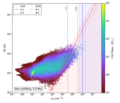
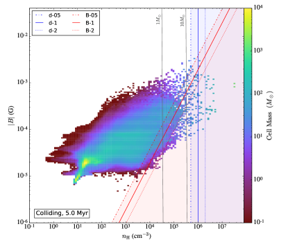
Figure 5: Phaseplots in $n_{\rm H}$ vs. $B$ space of the non-colliding (left panel) and colliding (right panel) cases at 5 Myr for non-star-forming models. The blue lines represent the star formation density threshold $n_{\rm H,sf}$ for the various critical densities in the density-regulated star formation routine. The blue-shaded region represents the regime in which star particles would form from these methods. The red lines represent the various mass-to-flux thresholds for the magnetically-regulated star formation routine, with the red-shaded region showing conditions needed for star particle formation. The black lines show the effective minimum densities due to the 50% mass limitation for two values of $m_{\rm\star,min}$.

The different star formation models can be directly compared via $|B|$ vs. ${n_{\rm H}}$ phaseplots (Figure 5). The critical thresholds for each model are plotted over phaseplots in respective non-colliding and colliding runs without star formation (i.e., fiducial runs from Paper II extended to $t=5.0~{}{\rm Myr}$). In this manner, the total mass along with various properties of the gas affected by each star formation model can be estimated. The colliding case forms regions of overall higher density and magnetization, both enhanced by approximately an order of magnitude. At a given density, gas in the colliding case generally contains stronger field strengths due to the nature of the compressive flows. The star formation thresholds for both the density-regulated and magnetically-regulated star formation routines are overplotted as blue and red lines, respectively.

The density-regulated star formation regime affects a greater total gas mass in the colliding case. As the critical density threshold decreases, the number of affected cells in both scenarios increases, leading to increased star formation regardless of magnetic field strength.

As the threshold for mass-to-flux ratio is lowered, a similar pattern of increasing star formation occurs. Key differences from the density-regulated models become apparent as star formation is now allowed to occur in regimes of low density, super-critical gas and is inhibited in high-density, sub-critical gas. Overall, the various models primarily create stars from the same gas, though narrow regimes exist in which stars form exclusively within certain routines. As discussed above, in these magnetically-regulated models, the effective minimum density thresholds for star formation provide an additional bound. In the $m_{\star,{\rm min}}=10~{}M_{\odot}$ models, much of the gas in the colliding cases–and even more so in the non-colliding cases–is limited by this effective density threshold. The $1~{}M_{\odot}$ cases allow star formation from a larger amount of locally super-critical gas. However, we will see below that the overall mass of stars formed by 5 Myr in the colliding case depends only weakly on this choice.

3.2 Properties of Star-forming Gas

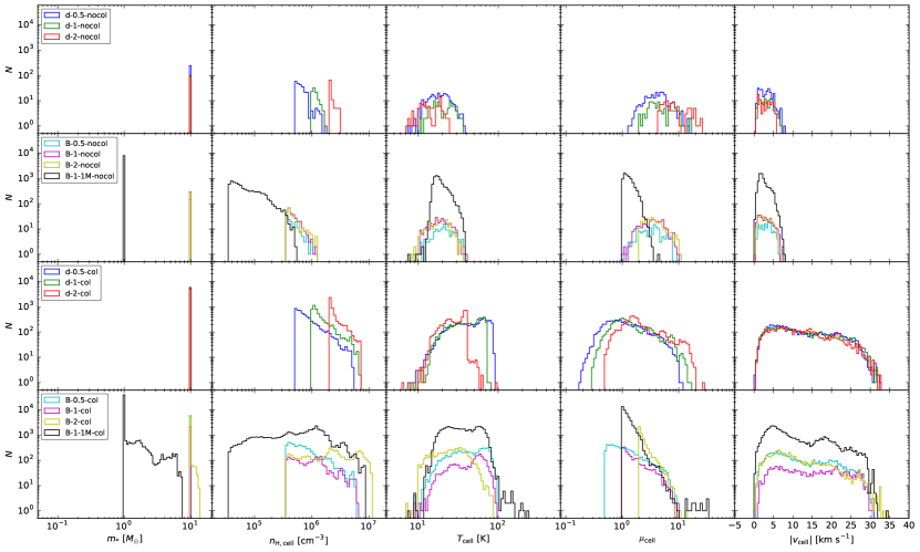
Figure 6: Masses of young stars and properties of star-forming gas cells. Histograms of (left to right) stellar mass, number density of the cells that form stars, gas temperature of such cells, normalized mass-to-flux ratio of such cells and velocity magnitude of such cells are shown for the non-colliding (top two rows) and colliding (bottom two rows) cases. The thresholds for critical densities and effective minimum densities can be seen as cutoffs for the density-regulated and magnetically-regulated star formation models, respectively. The critical mass-to-flux values can also be seen for the magnetically-regulated models.

We examine the masses of young stars and properties of their progenitor gas cells, just before a star particle is created. Figure 6 displays the cumulative histograms over 5 Myr of the stellar masses and key properties of the star-forming gas.

For the non-colliding cases, the stars form strictly at their threshold masses, indicating purely stochastic star formation is occurring. The density-regulated models form approximately 100-250 stars each, with higher critical density thresholds resulting in fewer stars. The distributions of cell densities peak at the thresholds of 0.5, 1, and $2\times 10^{6}\>{\rm cm^{-3}}$ for the respective models and extend above the cutoffs by factors of a few. Gas temperatures range from 6 to 40 K, averaging approximately 10 to 20 K with higher density thresholds resulting in slightly lower temperatures. The local normalized mass-to-flux ratio of the star-forming cells in these models is supercritical by factors of few for d-0.5-nocol to few tens for d-2-nocol. The velocities of these cells are generally a few ${\rm km~{}s^{-1}}$, consistent with values expected from decaying turbulence in the self-gravitating GMCs.

The magnetically-regulated non-colliding models exhibit slightly higher numbers of stars (few hundred for the $m_{\star,{\rm min}}=10~{}M_{\odot}$ models). Across these three models, distributions for density have peaks at the cutoff of $\sim 3\times 10^{5}\>{\rm cm^{-3}}$, temperatures primarily near 20 K (slightly above equilibrium), $\mu_{\rm cell}$ near 3-5 (slightly supercritical), and $|v|$ near 2 ${\rm km\>s^{-1}}$ (supersonic but consistent with decay of the initial turbulence). There exist slight trends of increasing density and decreasing temperature as the thresholds for $\mu_{\rm cell}$ increase between models. For the $m_{\star,{\rm min}}=1~{}M_{\odot}$ model, approximately 20 times more star particles are created. The distribution of cell densities also exhibit a cutoff at the effective minimum density of $\sim 3\times 10^{4}\>{\rm cm^{-3}}$ in this model, with the spread of densities reaching up to a factor of 20 higher. The temperature and velocity distributions exhibit similar peaks and spreads as their higher minimum stellar mass counterparts. However, the cells generally have a lower $\mu_{\rm cell}$ near 1 (magnetically critical) when stars are formed. This suggests that the condition for criticality is reached before the cell density grows to a point at which it can produce more massive stars in a given timestep and so stays in the stochastic limit.

The colliding models with density-regulated star formation produce $\sim 6\times 10^{3}$ stars, over 20 times the number formed from the non-colliding models over the same time period. The density distributions are similar to the non-colliding cases, peaking at the cutoffs, but exhibit an increased spread with cells reaching densities higher by factors of a few. The gas temperatures are also higher, averaging near 30-40 K but with a few cells reaching $\sim 90~{}{\rm K}$. Temperatures are generally lower for the higher-density cutoff models, but all peak at temperatures higher than equilibrium, likely due to shocks produced throughout the primary colliding region. The collision also produces high-density gas at a wide range of $\mu_{\rm cell}$, ranging from a few times subcritical up to $\sim 20$ times supercritical. The distributions peak near the value for magnetic criticality, with lower higher-density cutoff models corresponding with higher values of $\mu_{\rm cell}$. Cell velocity distributions are nearly identical, peaking near 10-20 ${\rm km\>s^{-1}}$.

For the magnetically-regulated colliding models with $m_{\star,{\rm min}}=10~{}M_{\odot}$, a similar star particle count is seen, exceeding their respective non-colliding models by factors of 10 to 20. The B-2-col model also forms some stars outside of the stochastic regime, as masses of $\sim{\rm 12-13}M_{\odot}$ are created. It is important to recall that the expected mass of the star particle to be created depends on the local SFR in the cell, i.e., on $\epsilon_{\rm ff}$ and the cell density, but also on the timestep of the simulation. Thus the presence and mass distribution of these higher mass star particles should not be over-interpreted. The presence of stars outside the stochastic regime simply indicates that some very high density, high SFR cells are present, and this is confirmed in the plots showing the density distributions, with some densities up to $n_{\rm H}=10^{7}~{}{\rm cm^{-3}}$. We note that star-forming cells can also have higher temperatures near 30 to 40 K, perhaps indicating creation of the dense gas in shocks, but recall that the star formation sub-grid model does not assess the degree of gravitational instability in the gas. The star-forming cells show a concentration of gas at the minimum magnetic criticality cutoff. They also exhibit generally higher velocities indicating strong turbulence and/or bulk motion associated with the GMCs.

The B-1-1M-col model has the greatest total number of stars formed, i.e., $\sim 5\times 10^{4}$ and forms a range of stellar masses up to $\sim 7~{}M_{\odot}$ (but again this mass function should not be expected to be compared to a real IMF, rather being simply the way the model ensures the total mass of stars formed is correct given the model parameters). Cell number densities range from $\sim 3\times 10^{4}$ to $\sim 9\times 10^{6}\>{\rm cm^{-3}}$. Temperatures are near 40 K and $\mu_{\rm cell}$ reaches a few tens but increases in cell number towards the critical value cutoff of 1. Velocities exhibit a similar trend as the $10~{}M_{\odot}$ models, showing high levels of turbulence, bulk motion, and/or infall to the primary cluster.

3.3 Star Formation Rates and Efficiencies

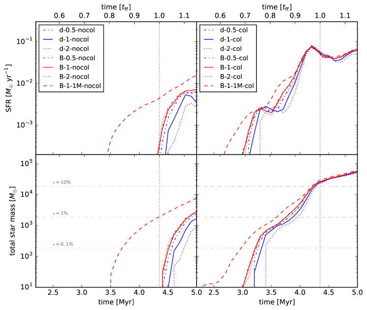
Figure 7: Top row: The star formation rates over time. The non-colliding cases are shown in the left column, while the colliding models are in the right column. Desity-regulated star formation models are traced with blue lines; magnetically-regulated models with red lines. The vertical dotted line shows the time after 1 free-fall time of the initial GMCs (see top axis). Bottom row: The total mass of stars formed versus time. The total star formation efficiency, shown for $\epsilon$=0.1%, 1%, and 10%, is normalized relative to the total initial mass within the two GMCs ($1.86\times 10^{5}\>M_{\odot}$).

The star formation rate (SFR) and overall star formation efficiency (SFE) of molecular clouds are important quantities that help determine the global galactic star formation process. The time evolution of these quantities for both non-colliding and colliding cases, for each star formation model, is shown in Figure 7.

The SFR is calculated as the time derivative of the total mass of the star particles. The efficiencies are determined by normalizing the total stellar mass by the combined gas mass of the two original GMCs. The evolution of these quantities is measured in simulation time, as well as relative to the freefall time of the initial GMC density ($t_{\rm ff}=4.35$ Myr).

In the non-colliding density-regulated cases, star formation initiates shortly after $1t_{\rm ff}$, i.e., at approximately $t=4.4$ Myr. The higher-cutoff density models form stars at slightly later times corresponding to when the critical density is achieved. At a given time, SFR and SFE vary by factors of a few between models. Over the course of the next 0.5 Myr (until simulation completion), the SFRs increase to $\sim(3-6)\times 10^{-3}\>M_{\odot}\>{\rm yr^{-1}}$ and then generally level off. Total stellar masses of $\sim 9\times 10^{2}-3\times 10^{3}\>M_{\odot}$ are created, corresponding to $\epsilon\approx 1\%$ by $1.15~{}t_{\rm ff}$.

For the magnetically-regulated cases with $m_{\rm\star,min}=10\>M_{\odot}$, star formation also starts after $1t_{\rm ff}$, and evolves in a similar manner as the density-regulated models except with slightly higher SFRs and efficiencies. The differences between these models is also much smaller, as the three $10~{}M_{\odot}$ magnetically-regulated models reach about $6\times 10^{-3}\>M_{\odot}\>{\rm yr^{-1}}$ by $1.1~{}t_{\rm ff}$ and then level off. The SFEs also reach and slightly exceed 1% by the simulation end time. The B-1-1M-nocol case exhibits the most dissimilar behavior of the non-colliding models, initiating star formation approximately 1 Myr earlier and reaching $4\times 10^{-3}\>M_{\odot}\>{\rm yr^{-1}}$ and $\epsilon=1\%$ by $1t_{\rm ff}$. By 5 Myr, the SFR and SFR are approximately 2-3 times greater than the other magnetically-regulated models.

The above trends are mostly likely caused by the fact that all these star formation models have effective density thresholds that need to be met to allow star formation to proceed, even the magnetically-regulated models (see §2.4.2). These thresholds decrease monotonically as we consider the density-regulated models, then the B-(0.5,1,2)-nocol models, and then the B-1-1M-nocol model. The simulations are in a regime in which the total SFR and eventual total SFE are set mostly by the fraction of gas in the GMCs that can meet these density threshold criteria. For the particular $B$-field strengths in these simulations (i.e., 10$\>{\rm\mu G}$), the choice of the magnetic threshold parameter does not play a significant role in setting the SFR.

The colliding cases produce much higher SFRs and SFEs during their evolution. The density-regulated models begin forming stars at a rapid pace shortly after $t=3.2$ Myr, with higher density thresholds slightly delaying the onset of star formation. There is some oscillation in the growth of the SFRs, but overall it increases from onset until $t_{\rm ff}$ near $0.08~{}M_{\odot}\>{\rm yr^{-1}}$ and then levels off through the culmination of the simulations. Star formation efficiencies reach 1% by 3.7 to 4 Myr and more than 20% by $t_{\rm ff}$. While the early behavior differs slightly in time between the density-regulated models, they appear to converge at later times.

The $m_{\rm\star,min}=10\>M_{\odot}$ magnetically-regulated colliding cases show very similar results to each other throughout the whole evolution, which indicates that the SFR is not limited by the mass-to-flux thresholds in this simulation set-up. Indeed, these models also converge with the density-regulated models by about 4 Myr. B-1-1M-col starts forming stars at the earliest times, but it also shows convergence in SFR by about 4 Myr. These results indicate that the SFR is in fact not limited by the density threshold criteria either. In the GMC-GMC collision the SFRs appear to be set by the creation of structures that can place gas at densities greater than any of the threshold densities, after which, even with $\epsilon_{\rm ff}=0.02$, it is turned quite efficiently into stars.

It is important to note that stellar feedback has not yet been included in our star formation models. Our current treatment may be a good approximation for initial SFRs, but mechanisms such as protostellar outflows that become important during formation, and ionization, winds and radiation pressure from massive stars soon after, will likely result in reduced SFRs.

3.4 Spatial Clustering

We investigate various quantitative metrics for spatial structure of the star clusters formed in our simulations. Global star and gas properties of the primary clusters are measured and the angular dispersion parameter (ADP) and minimum spanning tree (MST) methods are used to analyze cluster substructure. The ADP is sensitive to angular substructure at chosen radii, while the MST determines the degree of overall centrally concentrated clustering.

In order to define the primary cluster within a given model, we use the Density-based spatial clustering of applications with noise (DBSCAN) algorithm (Ester et al., 1996). This density-based clustering algorithm is applied to our projected star particle data and the median particle position of the highest population cluster is used as our initial cluster center. A circular aperture with initial radius of 0.4 pc is centered at this point, and a new center is determined by finding the center of mass using stars included only within this aperture. This process is repeated with aperture radii iteratively decreasing by factors of two, down to length scales of 0.1 pc. The ADP is found for the primary cluster using each of these defined centers, while the MST is found for the entire domain.

3.4.1 Global structure of primary cluster

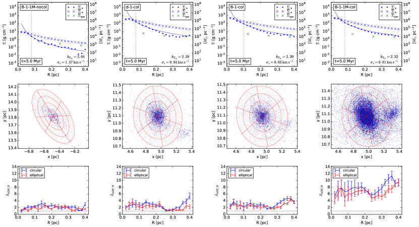
Figure 8: Top row: Mass surface densities as a function of radius for stars ($\Sigma_{\star}$) and gas ($\Sigma_{\rm gas}$) composing the primary clusters in various models at $t=5.0$ Myr. From left to right the models shown are B-1-1M-nocol, d-1-col, B-1-col and B-1-1M-col. Blue circles indicate $\Sigma_{\star}$ calculated locally in each circular annulus, while blue crosses show the enclosed average quantity, $\overline{\Sigma}_{*}$. A power law fit to $\Sigma_{\star}$ is shown as the blue line and the resulting exponent $k_{\Sigma_{\star}}$ is displayed. The black dotted line denotes the position of the stellar half-mass radius, $R_{1/2}$. The green crosses indicate the average enclosed gas mass, $\overline{\Sigma}_{\rm gas}$. The 1-D velocity dispersion of the stars, $\sigma_{z,1/2}$, is calculated for the cluster defined by the half-mass radius. Middle row: Visualization of the primary clusters. The star particles are shown as blue points, while the elliptical annuli and sectors used to calculate the angular dispersion parameter, $\delta_{\rm ADP,N}$, are overlaid in gray. Note that, for clarity, circular annuli that are used in calculating both the cluster profiles (top row) and for one version of the $\delta_{\rm ADP,N}$, are not displayed. Each sector is outlined in red, while the annuli are shown as gray ellipses with every fifth annulus highlighted in red. Bottom row: $\delta_{\rm ADP,6}$ vs. radius from the chosen cluster center. The values are calculated using both circular and elliptical annuli and averaged over twenty $3^{\circ}$ rotations of orientation of the 6-sector pattern. The error bars depict the standard error of the mean. A purely random azimuthal distribution of particles is indicated by the dotted line at $\delta_{\rm ADP,6}=1$.

We measure global structural properties of the primary star clusters created in the simulations. Figure 8 shows results for these clusters that have formed by $t=5~{}{\rm Myr}$ in four models: B-1-1M-nocol, d-1-col, B-1-col, and B-1-1M-col. Due to relatively sparse particle density, the clusters in the non-colliding $m_{\rm\star,min}=10\>M_{\odot}$ models were not included in this analysis. Also note that while elliptical annuli are displayed (see ADP discussion in Section 3.4.2), global properties for cluster structure are calculated using circular annuli.

The top row of Figure 8 shows the mass surface density of stars locally within each annulus, $\Sigma_{\star}$, the enclosed average mass surface density of stars, $\overline{\Sigma}_{\star}$, and the enclosed average mass surface density of the gas, $\overline{\Sigma}_{\rm gas}$. For the non-colliding case, $\overline{\Sigma}_{\star}$ ranges from about $10^{3}$ to $5\times 10^{4}~{}{\rm M_{\odot}\>pc^{-2}}$, whereas the colliding cases form clusters with approximately $10^{5}$ to $10^{6}~{}{\rm M_{\odot}\>pc^{-2}}$. It can be seen that $\Sigma_{\star}$ falls off quickly, reaching $\sim 10^{2}$ and $\sim 10^{4}~{}{\rm M_{\odot}\>pc^{-2}}$ by $R=0.4~{}{\rm pc}$ for non-colliding and colliding cases, respectively. We find best fit power law profiles of the form:

$$\Sigma_{*}(R)=A\left(\frac{R}{0.2~{}{\rm pc}}\right)^{-k_{\Sigma_{*}}},$$ (7)

where $A$ is a normalization factor, $R$ is the distance from cluster center, and $k_{\Sigma_{\star}}$ is the power law exponent. $k_{\Sigma_{\star}}$ is found to be $\sim 2.3$ to 2.6 for these primary clusters.

We denote a half-mass radius, $R_{1/2}$, as the radius within which half of the total mass of the cluster out to $R=0.4~{}{\rm pc}$ is contained. Within our chosen clusters, $R_{1/2}\simeq 0.08$-0.1 pc. Within $R_{1/2}$, the total enclosed stellar masses are $4.0\times 10^{2}\>M_{\odot}$, $2.3\times 10^{4}\>M_{\odot}$, $2.3\times 10^{4}\>M_{\odot}$, and $2.2\times 10^{4}\>M_{\odot}$ for models B-1-1M-v00, d-1-v10, B-1-v10, and B-1-1M-v10, respectively. This shows that the properties of the primary cluster in the colliding simulations are not much affected by the choice of star formation subgrid model. Within $R_{1/2}$, the averaged stellar mass surface density is $\overline{\Sigma}_{*,1/2}=2.1\times 10^{4}\>{\rm M_{\odot}~{}pc^{-2}}$ ($4.4\>{\rm g~{}cm^{-2}}$) for the non-colliding case and $1.1\times 10^{6}\>{\rm M_{\odot}~{}pc^{-2}}$ ($2.28\times 10^{2}\>{\rm g~{}cm^{-2}}$), $8.0\times 10^{5}\>{\rm M_{\odot}~{}pc^{-2}}$ ($1.7\times 10^{2}\>{\rm g~{}cm^{-2}}$), and $1.06\times 10^{6}~{}{\rm M_{\odot}\>pc^{-2}}$ ($2.22\times 10^{2}\>{\rm g~{}cm^{-2}}$) for the respective colliding GMC models. The respective gas masses are $53\>M_{\odot}$, $5.7\times 10^{2}\>M_{\odot}$, $7.7\times 10^{2}\>M_{\odot}$, and $4.5\times 10^{2}\>M_{\odot}$. Note that the $\sim 0.1~{}{\rm pc}$ scales are barely resolved in our simulation, so only the average enclosed gas masses are measured. At this stage, the cluster in the non-colliding case has $\Sigma_{\rm\star}<\overline{\Sigma}_{\rm gas}$. The colliding cases all have $\Sigma_{\rm\star}>\overline{\Sigma}_{\rm gas}$.

We compare these cluster properties with those of observed young clusters (see, e.g., Figure 1 of Tan et al., 2014). The cluster formed in the non-colliding simulation B-1-1M-v00 that has $\overline{\Sigma}_{\star}\simeq 2\times 10^{4}~{}M_{\odot}\>{\rm pc^{-2}}$ ($4.4\>{\rm g~{}cm^{-2}}$) is much denser than any known young cluster of comparable mass (i.e., with $M_{*,1/2}\lesssim 1000\>M_{\odot}$). The colliding simulations produce more massive clusters and these are also seen to have much higher mass surface densities (by more than a factor of ten) at their half-mass scale than the densest known Galactic clusters, such as the Arches or Westerlund 1. We note that stellar feedback is not currently included within our simulations and expect the implementation of protostellar outflow feedback, planned in a future paper, to result in a reduction of $\overline{\Sigma}_{\star}$.

The 1-D velocity dispersion, $\sigma_{z,1/2}$, is calculated for the stars seen to be within projected radii of $R_{1/2}$. The cluster formed in the non-colliding case has $\sigma_{z,1/2}=1.57\>{\rm km\>s^{-1}}$, while those formed from GMC collisions have much higher values of 9.94, 9.83, and $8.81\>{\rm km\>s^{-1}}$, respectively for these clusters shown in Figure 8 (left to right). More detailed kinematic analysis is performed in Section 3.5.

The dynamical state of the clusters is investigated via calculation of the virial ratio,

$$Q_{i}=-\frac{T_{\star}}{\Omega} = \frac{3\sigma^{2}R}{2GM_{\star}},$$ (8)

where $T_{\star}$ and $\Omega$ are the total kinetic and gravitational potential energies of the stars, respectively. For a given radius $R$, $M_{\star}$ is the total enclosed stellar mass and $\sigma$ is the 1-D velocity dispersion of the enclosed particles. Values of $Q_{i}<1$ indicate a bound cluster, while $Q_{i}=0.5$ represents a state of virial equilibrium.

We find virial ratios at $R_{1/2}$ of 0.34, 0.24, 0.29, and 0.19 for the primary clusters from the simulations B-1-1M-v00, d-1-v10, B-1-v10, and B-1-1M-v10, respectively. These are all sub-virial, with collisions forming more tightly bound clusters at this stage in their evolution. However, as noted in §2.4.3, due to $R_{1/2}$ approaching the grid scale, gravitational forces are not well resolved and thus accurate dynamical evolution of the cluster is limited. When the virial ratio is calculated at better-resolved scales of $R=0.4~{}{\rm pc}$, we find increased values of 0.44, 0.38, 0.36, and 0.33 for the same clusters, respectively.

3.4.2 Angular Dispersion Parameter

The angular dispersion parameter (ADP), $\delta_{\rm ADP,N}(R)$ (Da Rio et al., 2014), is a technique for quantifing the degree of substructure of a stellar distribution, especially designed for application to centrally-concentrated star clusters. It is similar to the azimuthal asymmetry parameter (AAP) developed by (Gutermuth et al., 2005). In its simplest form, this technique divides the distribution spatially into equal-area circular sectors and compares the dispersion of the number counts contained within each region. Further division using concentric annuli allows study of this substructure as a function of radius. In order to account for a global elongation or eccentricity of the cluster, best-fitted elliptical annuli can be used. We will adopt this as our fiducial method. To obtain the best-fit ellipse shape and orientation, a linear fit to the stars projected in the central 0.2 pc of the cluster is used to set the position angle, $\theta_{e}$ of the semi-major axis, $a$. Then the dispersion in position in directions parallel and perpendicular to $\theta_{e}$ are calculated to derive the eccentricity. For results in a given annulus of semi-major axis, $a$, we display them at a radius, $R$, for which the circular area would be equal to that of the ellipse.

For a given annulus divided into a total of $N$ equal sectors, each $i$th sector contains $n_{i}$ stars. The ADP is defined as:

$$\delta_{\rm ADP,N}=\sqrt{\frac{1}{(N-1)\overline{n}}\sum\limits_{i=1}^{N}(n_{i}-\overline{n})^{2}}=\sqrt{\frac{\sigma^{2}}{\sigma^{2}_{\rm Poisson}}},$$ (9)

where $\sigma$ is the standard deviation of the $n_{i}$ values, $\overline{n}$ is the average of the number of stars per sector in the given annulus, and $\sigma_{\rm Poisson}$ is the standard deviation expected from a Poisson distribution. Thus, values of $\delta_{\rm ADP,N}\simeq 1$ indicate nearly random distributions of sources, azimuthally.

ADP analysis was performed using 20 equally-spaced concentric annuli out to a maximum radius of 0.4 pc with $N=6$ equally-divided sectors. $\delta_{\rm ADP,6}$ is computed for twenty orientations of the sector pattern at every $3^{\circ}$ angular rotation, and the final value is averaged. Both circular and elliptical annuli are used to calculate $\delta_{\rm ADP,6}$, using the same previously determined cluster center.

The star cluster formed in the non-colliding model, which has a relatively low number of stars and thus larger Poisson errors, has $\delta_{\rm ADP,6}\simeq$ 1.5 - 2.5 for circular annuli and $\simeq 1$ - 2 for elliptical annuli. In both cases, $\delta_{\rm ADP,6}$ peaks near $R=0.15~{}{\rm pc}$.

The primary clusters from the colliding models have similar morphologies, especially the density-regulated and magnetically-regulated $m_{\rm\star,min}=10~{}M_{\odot}$ cases. In the B-1-1M-col model, there exists a denser population of lower mass stars and the location of the subcluster $R=0.4~{}{\rm pc}$ is at a slightly different position. This slight deviation may be attributed to the earlier onset of star formation from lower density gas.

The circular and elliptical $\delta_{\rm ADP,6}$ values are similar, although again the latter is slightly smaller in size. For the clusters in the d-1-col and B-1-col simulations, $\delta_{\rm ADP,6}\simeq 2$-3, while the B-1-1M-col model has overall higher values of $\delta_{\rm ADP,6}\simeq 6$-7. The radial behavior of the clusters from the three colliding models is similar as well, in that the cluster has moderate values of $\delta_{\rm ADP,6}$ out to $R\approx 0.2~{}{\rm pc}$. These decrease at the outskirts of the defined cluster, then increase relatively sharply out to $R\approx 0.4~{}{\rm pc}$ upon the presence of the subcluster.

Da Rio et al. (2014) carried out a similar ADP analysis of the Orion Nebula Cluster (ONC). They found $\delta_{\rm ADP,N}$ with $N=4,6,9$ rises from below 1 in the very center of the ONC to reach fairly constant values of about 1.5 to 2.5 from 0.1 pc to about 1.3 pc. Accounting for ellipticity in the annuli brings these values of $\delta_{\rm ADP,N}$ down to about 1 to 1.5, with some variations near 2. Da Rio et al. concluded the projected spatial distribution of young, embedded stars in the ONC is relatively smooth, which may be evidence for dynamical processing if the cluster is older than a few orbit crossing times.

The primary cluster formed in the B-1-1M-nocol model returns similar values of $\delta_{\rm ADP,6}$ as the ONC, while the $m_{\rm\star,min}=10~{}M_{\odot}$ colliding models return slightly higher values. The B-1-1M-col case has much higher $\delta_{\rm ADP,6}$, which may be attributed to its much larger number of stars ($\sim 10$ times higher) resulting in smaller Poisson errors. As discussed in §2.4.3, we caution that the simulation code is not able to resolve small scale gravitational interactions between stars, potentially affecting the outcome of this metric. Still, we expect future application of this technique to better resolved clusters, including models where final stellar concentrations are reduced by including local feedback, will provide useful comparisons with observed young, embedded clusters to help test different formation scenarios.

3.4.3 Minimum spanning tree

Another method of studying the hierarchical structure of stellar distributions is through the use of the minimal spanning tree (MST). The MST (developed for astrophysical applications by Barrow et al., 1985) is a technique borrowed from graph theory in which all of the vertices of a connected, undirected graph are joined such that the total weighting for the graph edges is minimized. In the case of star clusters, the projected euclidean distances between the individual stars acts as the edge weight.

To study the hierarchical structure of a collection of stars, Cartwright & Whitworth (2004) introduced a dimensionless parameter, $Q$, which can distinguish and quantify between smooth radial clustering (i.e., more centrally concentrated) vs. multi-scale type clustering (i.e., more substructure). Specifically,

$$Q=\frac{\overline{s}}{\overline{m}}.$$ (10)

The numerator is the normalized correlation length

$$\overline{s}=\frac{\overline{d}}{R_{\rm cluster}},$$ (11)

where $\overline{d}$ is the mean pairwise separation distance between the stars and $R_{\rm cluster}$ is the overall cluster radius, calculated as the distance from the mean position of all stars to the farthest star. The denominator is the normalized mean edge length

$$\overline{m}=\sum_{i=1}^{N_{\star}-1}\frac{e_{i}}{\sqrt{(N_{\star}A)(N_{\star}-1)}},$$ (12)

where $N_{\star}-1$ is the total number of edges, $e_{i}$ is the length of each edge, and $A=\pi R_{\rm cluster}^{2}$ is the cluster area.

Table 3: Parameters of Observed Clusters

Cluster		$Q$		$\overline{s}$		$\overline{m}$
Taurus		0.47		0.55		0.26
IC2391		0.66		0.74		0.49
Chameleon		0.67		0.63		0.42
$\rho$ Ophiuchus		0.85		0.53		0.45
IC348		0.98		0.49		0.48

The threshold of $Q_{0}=0.785$ determines a quantitative threshold of either smooth radial clustering ($Q>Q_{0}$) or multi-scale clustering ($Q<Q_{0}$). Table 3 lists $Q$, $\overline{s}$, and $\overline{m}$ for various observed clusters (see, e.g., Cartwright & Whitworth, 2004).

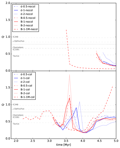
Figure 9: Minimum spanning tree $Q$ parameter vs. time. The evolution of $Q$ is shown for each non-colliding (top) and colliding (bottom) model, as denoted. The values of $Q$ are averaged over the three cardinal lines of sight, $x$, $y$, and $z$. The dotted black line denotes the threshold of $Q_{0}=0.785$, denoting smooth radial ($Q>Q_{0}$) vs multi-scale ($Q<Q_{0}$) clustering. The gray dashed lines show values of $Q$-parameters of various observed star clusters from Table 3.

We track the evolution of $Q$ throughout our simulations (see Figure 9). In the $m_{\rm\star,min}=10\>M_{\odot}$ non-colliding cases, clustering begins with $Q\approx 0.5$, at the low end of observed clusters (e.g., Taurus), and continues to decrease monotonically. For B-1-1M-nocol, an initially much higher $Q$ is seen, but this quickly decreases to values even lower than the other cases. This general behavior can be understood as the formation of an initial cluster (more tightly concentrated in the $m_{\rm\star,min}=1\>M_{\odot}$ case). However, the overall stellar distribution soon appears very dispersed as other independent clusters form throughout the GMCs.

The colliding cases exhibit very different behavior. The density-regulated cases begin with similar $Q$ parameter values and initially decrease from 0.5 to 0.25. However, beginning near 3.4 Myr, they experience a sharp increase in $Q$, reaching between 0.8 and 1.2, corresponding with the high end of observed clusters (e.g., $\rho$ Ophiuchus and IC348). The higher-density cutoff models reach higher maximum $Q$ values and peak at later times. After this peak, the $Q$ values drop to fairly multi-scale-type clustering, but then rise again toward 0.5 to 0.7 in the final 0.5 Myr. The $m_{\rm\star,min}=10\>M_{\odot}$ magnetically-regulated cases have similar qualitative behavior, with the $Q$ peak occurring earlier in time, near 3.6 Myr and reaching very large values, surpassing centrally clustered observations. However, $Q$ also drops down to $\sim 0.25$ but again equalizes to values near 0.6. These can be understood as the initial formation of a moderately distributed star cluster which quickly becomes very centrally dominated as a result of new star formation in the compressed gas due to the collision that forms a primary cluster. However, the colliding region soon produces other clusters separated from the primary star cluster, thus decreasing $Q$. Then, beginning from $t\approx 4.0$ Myr, the gas and stars continue to coalesce, growing in size, number of stars, and central concentration. The primary cluster grows and accumulates more of the surrounding clusters, leading to the growth into a slightly multi-scale distribution overall. The B-1-1M-col model begins near $Q=0.6$ and experiences a lower peak near 0.8 before dropping off to 0.25. The final rise of $Q$ is concurrent with the other colliding models, but instead of settling near 0.6, $Q$ continues to rise until the end of the simulation $t=5.0$ Myr, reaching a very high central clustering value of 1.5.

When comparing the results from our non-colliding vs. colliding simulations, clusters formed by GMC collisions spend a much greater fraction of the initial 5 Myr evolution with $Q$ parameters within the range of observed clusters. While this result should not be overinterpreted, as clusters produced in the non-colliding cases may evolve into more centrally peaked distributions at beyond 5 Myr, a much stronger clustering of stars naturally arises from colliding gas, and this behavior is quantitatively realized in our simulations.

3.5 Gas and Star Kinematics

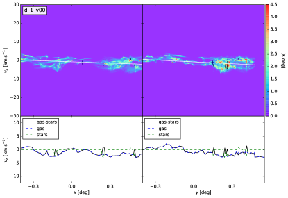
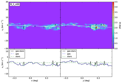
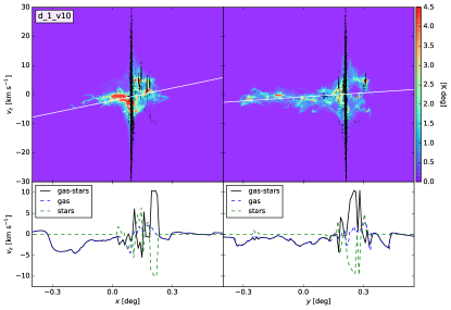
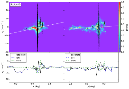
Figure 10: Position-velocity diagrams for selected non-colliding (top row) and colliding (bottom row) simulations for the density-regulated (left column) and magnetically-regulated (right column) star formation routines. Each model is shown at $t=5.0\>{\rm Myr}$ along the $z$ line of sight. The colormap depicts synthetic ¹³CO($J$=1-0) line intensities from the gas through velocity bins of $\Delta v=0.212\>{\rm km\>s^{-1}}$. The star particles are overplotted as black points. The gray cross indicates the position of the center of mass and the solid white line shows the intensity-weighted linear velocity gradient ($dv_{\rm los}/ds$) across each cloud. Below each respective position-velocity diagram are plots of the mean gas velocity, mean star velocity, and their difference. Positional bins of $0.5~{}{\rm pc}$ (i.e., $9.5\times 10^{-3}~{}{\rm deg}$ for an adopted system distance of 3 kpc) are used.

The relationship between the kinematics of young stars and their surrounding gas has been studied in order to gain insight into the formation and early evolution of young, embedded stellar populations. For example, using data from the INfrared Spectra of Young Nebulous Clusters (IN-SYNC) survey (Cottaar et al., 2014), which achieves radial velocity accuracies of about 0.3 $\rm km\>s^{-1}$, Foster et al. (2015) have studied the kinematic properties of young stars in NGC 1333, while Cottaar et al. (2015) have carried out a similar analysis of IC 348. Da Rio et al. (2017) (see also Hacar et al., 2016; Stutz & Gould, 2016) analyzed similar data for the ONC and its extended southern filament, including comparison to gas tracers such as ¹³CO. Our simulations allow a similar investigation of the kinematic properties of both ¹³CO-defined gas and the young stars under various star formation scenarios.

Our gas structures are defined using synthetic ¹³CO($J$=1-0) emission, based on the same observational assumptions as Paper II (i.e., GMCs are at a distance $d$=3 kpc, the optically thin limit applies, and we bin with a spectral resolution of $0.212~{}{\rm km\>s^{-1}}$). Figure 10 shows position-velocity diagrams for non-colliding and colliding cases for density and magnetically-regulated star formation models (such analysis methods have also been carried out in the simulations of Duarte-Cabral et al., 2011; Dobbs et al., 2015; Butler et al., 2015; Haworth et al., 2015a). The mean gas velocity, mean stellar velocity, and difference in these means as functions of position are also shown as profiles plotted below their respective colormaps. Mean values are taken using positional bins of 0.5 pc (i.e., $9.5\times 10^{-3}~{}{\rm deg}$).

The non-colliding cases show widely dispersed gas over the positional space, with clumpy morphology in ¹³CO($J$=1-0). The velocity $v_{z}$ is fairly low, staying within $\pm 5~{}{\rm km\>s^{-1}}$. The gas velocity gradient is relatively shallow, following the general structure of the clouds. The gas and stellar kinematics in the density-regulated and magnetically-regulated star formation models are similar, with more star clusters present in the B-1-v00 model. The star clusters can be seen localized in positional space with a small scatter in velocity space. Generally, the stars are positioned in the vicinity of other high-intensity ¹³CO clumps.

The colliding cases show very different behavior in position-velocity space. The gas is much more localized spatially in $x$, the direction of the colliding flows. The structure is more concentrated in the $y$-direction as well due to the higher central gravitational potential formed. The average ¹³CO-weighted velocity gradient is much steeper in $x$ for the colliding cases, but relatively similar in magnitude to the non-colliding cases in the $y$ line of sight. Larger clumps with higher intensities of ¹³CO gas are seen in the colliding cases, with a dense network of filamentary structures present. Additionally, the gas velocity dispersion is much greater, with portions reaching velocity dispersions of $\pm 20~{}{\rm km\>s^{-1}}$. Gas and stellar kinematic morphologies are also similar among the different star formation models. The central star cluster is seen to have a very large velocity dispersion, with the primary clusters in d-1-col and B-1-col models found in § 3.4.1 to have $\sigma_{z,1/2}=9.94$ and $9.83~{}{\rm km\>s^{-1}}$, respectively. Separate, smaller clusters can also be seen with their own stellar populations near high-intensity clumps of gas.

Table 4: Gas and Star Kinematics

Case	LoS	$\frac{dv_{\rm los}}{ds}$	$\sigma_{\rm gas}$	$\sigma_{*}$	$\overline{v}_{\rm gas}$	$\overline{v}_{*}$	$\Delta\overline{v}$
		($\rm{km\>s^{-1}\>pc^{-1}}$)	($\rm{km\>s^{-1}}$)	($\rm{km\>s^{-1}}$)	($\rm{km\>s^{-1}}$)	($\rm{km\>s^{-1}}$)	($\rm{km\>s^{-1}}$)
d-1-v00	$x$	0.096	1.810	1.700	1.024	0.705	0.319
	$y$	0.017	1.271	1.179	-0.124	-0.657	0.533
	$z$	0.077	2.107	1.882	-1.189	-1.358	0.169
	RMS	0.072	1.763	1.615	0.909	0.961	0.372
B-1-v00	$x$	0.096	1.810	1.777	1.022	0.554	0.467
	$y$	0.017	1.275	1.349	-0.124	-0.343	0.220
	$z$	0.079	2.110	2.055	-1.188	-1.450	0.261
	RMS	0.072	1.766	1.751	0.908	0.918	0.334
d-1-v10	$x$	0.194	4.087	8.301	-0.305	0.810	-1.115
	$y$	0.278	4.428	10.427	0.566	-1.344	1.909
	$z$	0.287	4.093	10.683	-0.583	-1.226	0.643
	RMS	0.256	4.206	9.862	0.501	1.150	1.330
B-1-v10	$x$	0.194	4.059	8.307	-0.324	0.881	-1.206
	$y$	0.288	4.408	9.989	0.567	-1.377	1.944
	$z$	0.293	4.104	10.170	-0.590	-1.171	0.582
	RMS	0.262	4.193	9.526	0.508	1.161	1.363

From the position-velocity information, we calculate velocity gradients of the gas ($\frac{dv_{\rm los}}{ds}$), the velocity dispersion of the gas ($\sigma_{\rm gas}$), the velocity dispersion of the stars ($\sigma_{\rm*}$), the ¹³CO-weighted average velocities of the gas ($\overline{v}_{\rm gas}$), the mass-weighted average velocities of the stars ($\overline{v}_{*}$), and the velocity offset between the two ($\Delta\overline{v}$). Table 4 summarizes these properties for the four models as viewed from $x$, $y$, and $z$ lines of sight, as well as their RMS values.

We note that the average $\sigma_{*}$ values (9.86 and 9.53 ${\rm km\>s^{-1}}$) in the whole domain are only slightly lower than those of the primary cluster (9.94 and 9.83 ${\rm km\>s^{-1}}$). In these cases, the central cluster contains the majority of the stars and thus dominates the overall distribution.

Within the non-colliding cases, both the gas and stellar kinematics agree fairly closely between different star formation models. The velocity gradients are larger in the $x$ and $y$ directions due to asymmetries from the impact parameter. A RMS value of $0.072~{}\rm{km\>s^{-1}\>pc^{-1}}$ is recorded. The dispersion of the gas and stars are similar in both models, with $\sigma_{\rm gas,RMS}\approx 1.76~{}\rm{km\>s^{-1}}$ and $\sigma_{\rm*,RMS}\approx 1.68~{}\rm{km\>s^{-1}}$. The mean velocities of the gas and stars are also similar, with $\overline{v}_{\rm gas,RMS}\approx 0.91~{}\rm{km\>s^{-1}}$ and $\overline{v}_{\rm*,RMS}\approx 0.94~{}\rm{km\>s^{-1}}$. The stellar velocities in the density-regulated model have slightly lower dispersions, but higher mean values. Overall, the velocity offset between the gas and the stars for the non-colliding models is approximately $0.35~{}\rm{km\>s^{-1}}$.

For the colliding cases, the density-regulated and magnetically-regulated star formation models exhibit similar kinematic properties of the gas and stars. On average, $\frac{dv_{\rm los}}{ds}=0.26~{}\rm{km\>s^{-1}\>pc^{-1}}$, $\sigma_{\rm gas,RMS}=4.14~{}\rm{km\>s^{-1}}$, $\sigma_{\rm*,RMS}=9.70~{}\rm{km\>s^{-1}}$, $\overline{v}_{\rm gas,RMS}=0.50~{}\rm{km\>s^{-1}}$, $\overline{v}_{\rm*,RMS}=1.16~{}\rm{km\>s^{-1}}$, and $\Delta\overline{v}=1.35~{}\rm{km\>s^{-1}}$. Relative to non-colliding clouds, the collision induces a much larger velocity gradient ($\sim$3-4 times greater), a larger velocity dispersion in the gas ($\sim$2 times greater), and a much larger stellar velocity dispersion ($\sim$5 times greater).

As functions of position, the mean velocities of gas, stars, and their offsets, are compared. Offsets exist in both non-colliding and colliding cases, becoming most apparent in close proximity to star clusters. For the non-colliding case, these differences are relatively small, at a few ${\rm km\>s^{-1}}$. However, the colliding case contains regions in which the offsets exceed $5~{}{\rm km\>s^{-1}}$. Averaged over position space, colliding GMCs result in velocity offsets a factor of $\sim$4 times higher than non-colliding GMCs. This parameter may be an indicator for determining the dynamical formation history of young star clusters, as results from collisions show more disturbance kinematically.

We make a first, simple comparison with the results of the IN-SYNC survey of the ONC and surroundings (Da Rio et al., 2017). This survey found offsets between gas and star velocities of approximately $\Delta v_{r}\sim-0.5$ km/s, but up to $-1.0$ to $-1.5$ km/s in some regions. The magnitude of such offsets are in general consistent with those seen in both the non-colliding and colliding models, especially considering variations associated with the particular line of sight. Given that the observational data for Orion is just a single example of a star-forming region, viewed on a particular sight line, it is difficult to draw definitive conclusions about whether the gas and star kinematics favor one scenario over another. Larger numbers of star-forming regions need to be studied with similar methods. In addition, other metrics, such as the comparison of low and high density gas tracers (e.g., Henshaw et al., 2013, 2014), need to be examined, which on the simulation side requires extension of the astrochemical modeling to include species such as $\rm N_{2}H^{+}$.

4 Discussion and Conclusions

We have implemented two classes of star formation sub-grid routines into the MHD code Enzo that we are using to study GMC collisions: a density-regulated model based on a threshold density and a new magnetically-regulated model based on a threshold mass-to-flux ratio. Varying key parameters for each star formation routine, we explored the large-scale morphology, properties of star-forming gas, global star formation rates and efficiencies over time, spatial clustering of the stars, and gas and stellar kinematics. For each model, we investigated scenarios of non-colliding and colliding GMCs.

The non-colliding cases evolved in a relatively quiescent manner, driven by the initial turbulence and interplay of self-gravity and magnetic fields. Star clusters formed only in the very late stages of the simulations, from overdense clumps located within filaments and dispersed throughout the GMC complex. Generally, these clusters contained hundreds of solar masses each and grew at a relatively slow rate. Star clusters in the density-regulated star formation routines were smaller and more isolated. The clusters formed in the magnetically-regulated models exhibited slightly more elongated morphologies. For this simulation set up, the level of star formation activity appears to be regulated by the effective density threshold that is used in each of these models, with the mass-to-flux criterion not having a large influence.

During collisions between GMCs, stars formed earlier and in larger clusters, from high-density gas produced in the primary filamentary colliding region. While star formation rates level off by the completion of the simulations, extrapolation of future behavior is unclear. Nevertheless, by $t=5~{}{\rm Myr}$, individual clusters have grown and merged to form one large, dominant cluster with a total stellar mass of $5\times 10^{4}~{}M_{\odot}$. For this particular set-up, the final overall level of star formation is relatively independent of all the explored star formation sub-grid models. Star formation appears to be limited by the ability of the collision to direct mass into high density regions, which then eventually form stars with high overall efficiency.

Just prior to star formation, both density and magnetically regulated star formation result in fairly similar gas properties of parent cells. However, colliding cases experience relatively wider ranges of densities, temperatures, $\mu_{\rm cell}$, and velocity magnitude. Higher mean values for density and temperature are found, while gas is more magnetically subcritical and turbulent.

The primary star clusters formed in the various models were analyzed and found to have much higher surface densities at their half-mass scale than any observed cluster. We expect the future inclusion of stellar feedback will reduce these surface densities. The angular dispersion parameter (ADP) analysis was carried out on the primary clusters in the simulations. ADP values are generally greater than those see in the ONC, which may indicate the ONC is dynamically older than the simulated clusters. The MST $Q$ parameter was also used to investigate the global spatial distribution properties of the star, with non-colliding cases resulting in overall highly multi-scaled clustering due to the scattered formation of independent clusters. Colliding GMCs produce clusters with $Q$ parameters that vary between those expected of multi-scale and centrally clustered distributions.

Kinematically, our colliding GMC cases produce velocity gradients 3-4 times greater than those of the non-colliding cases. The velocity dispersions also differ, with the gas in the colliding clouds having approximately twice the velocity dispersion. Stellar velocity dispersions in the simulations are dominated by the potentials of the primary clusters that form, with this leading to much greater dispersions in the colliding case. We find that the colliding cases produce typically 4 times larger offsets between the mean gas and mean star velocities compared to the non-colliding case.

Finally, we remind the reader of several important caveats. The young stars do not inject feedback, especially protostellar outflow feedback, into the surrounding gas. Internal star cluster dynamics are not well followed because of gravitational softening at the grid scale ($\sim 0.1$ pc) and because the star particles lack realistic mass and multiplicity distributions. Still the conditions that are simulated here may provide boundary conditions for more detailed models that are able to follow full $N$-body evolution of the clusters (e.g., Farias et al., 2017). Finally, in the context of GMC collisions, a wide range of cloud (e.g., degree of initial magnetization) and collision (e.g., velocities; impact parameters) parameters remain to be explored with these models. These items will be addressed in subsequent papers in this series.

References

- Anathpindika (2009) Anathpindika, S. 2009, A&A, 504, 437
- Balfour et al. (2015) Balfour, S. K., Whitworth, A. P., Hubber, D. A., & Jaffa, S. E. 2015, MNRAS, 453, 2471
- Barrow et al. (1985) Barrow, J. D., Bhavsar, S. P., & Sonoda, D. H. 1985, MNRAS, 216, 17
- Bryan et al. (2014) Bryan, G. L., Norman, M. L., O’Shea, B. W., et al. 2014, ApJS, 211, 19
- Butler & Tan (2009) Butler, M. J., & Tan, J. C. 2009, ApJ, 696, 484
- Butler & Tan (2012) —. 2012, ApJ, 754, 5
- Butler et al. (2015) Butler, M. J., Tan, J. C., & Van Loo, S. 2015, ApJ, 805, 1
- Cartwright & Whitworth (2004) Cartwright, A., & Whitworth, A. P. 2004, MNRAS, 348, 589
- Chira et al. (2013) Chira, R.-A., Beuther, H., Linz, H., et al. 2013, A&A, 552, A40
- Cottaar et al. (2014) Cottaar, M., Covey, K. R., Meyer, M. R., et al. 2014, ApJ, 794, 125
- Cottaar et al. (2015) Cottaar, M., Covey, K. R., Foster, J. B., et al. 2015, ApJ, 807, 27
- Crutcher (2012) Crutcher, R. M. 2012, ARA&A, 50, 29
- Da Rio et al. (2014) Da Rio, N., Tan, J. C., & Jaehnig, K. 2014, ApJ, 795, 55
- Da Rio et al. (2017) Da Rio, N., Tan, J. C., Covey, K. R., et al. 2017, ArXiv e-prints, arXiv:1702.04113
- Dedner et al. (2002) Dedner, A., Kemm, F., Kröner, D., et al. 2002, Journal of Computational Physics, 175, 645
- Dobbs et al. (2015) Dobbs, C. L., Pringle, J. E., & Duarte-Cabral, A. 2015, MNRAS, 446, 3608
- Duarte-Cabral et al. (2011) Duarte-Cabral, A., Dobbs, C. L., Peretto, N., & Fuller, G. A. 2011, A&A, 528, A50
- Ester et al. (1996) Ester, M., Kriegel, H., Sander, J., & Xu, X. 1996, in (AAAI Press), 226–231
- Farias et al. (2017) Farias, J. P., Tan, J. C., & Chatterjee, S. 2017, ArXiv e-prints, arXiv:1701.00701
- Few et al. (2016) Few, C. G., Dobbs, C., Pettitt, A., & Konstandin, L. 2016, MNRAS, 460, 4382
- Foster et al. (2015) Foster, J. B., Cottaar, M., Covey, K. R., et al. 2015, ApJ, 799, 136
- Fujimoto et al. (2014) Fujimoto, Y., Tasker, E. J., & Habe, A. 2014, MNRAS, 445, L65
- Ginsburg et al. (2012) Ginsburg, A., Bressert, E., Bally, J., & Battersby, C. 2012, ApJ, 758, L29
- Gutermuth et al. (2005) Gutermuth, R. A., Megeath, S. T., Pipher, J. L., et al. 2005, ApJ, 632, 397
- Habe & Ohta (1992) Habe, A., & Ohta, K. 1992, PASJ, 44, 203
- Hacar et al. (2016) Hacar, A., Alves, J., Forbrich, J., et al. 2016, A&A, 589, A80
- Haworth et al. (2015a) Haworth, T. J., Shima, K., Tasker, E. J., et al. 2015a, MNRAS, 454, 1634
- Haworth et al. (2015b) Haworth, T. J., Tasker, E. J., Fukui, Y., et al. 2015b, MNRAS, 450, 10
- Heitsch et al. (2009) Heitsch, F., Stone, J. M., & Hartmann, L. W. 2009, ApJ, 695, 248
- Henshaw et al. (2014) Henshaw, J. D., Caselli, P., Fontani, F., Jiménez-Serra, I., & Tan, J. C. 2014, MNRAS, 440, 2860
- Henshaw et al. (2013) Henshaw, J. D., Caselli, P., Fontani, F., et al. 2013, MNRAS, 428, 3425
- Inutsuka et al. (2015) Inutsuka, S.-i., Inoue, T., Iwasaki, K., & Hosokawa, T. 2015, A&A, 580, A49
- Jaehnig et al. (2015) Jaehnig, K. O., Da Rio, N., & Tan, J. C. 2015, ApJ, 798, 126
- Klein & Woods (1998) Klein, R. I., & Woods, D. T. 1998, ApJ, 497, 777
- Kong et al. (2017) Kong, S., Tan, J. C., Caselli, P., et al. 2017, ArXiv e-prints, arXiv:1701.05953
- Krumholz & McKee (2005) Krumholz, M. R., & McKee, C. F. 2005, ApJ, 630, 250
- Krumholz & Tan (2007) Krumholz, M. R., & Tan, J. C. 2007, ApJ, 654, 304
- Lim & Tan (2014) Lim, W., & Tan, J. C. 2014, ApJ, 780, L29
- Ma et al. (2013) Ma, B., Tan, J. C., & Barnes, P. J. 2013, ApJ, 779, 79
- Mouschovias & Spitzer (1976) Mouschovias, T. C., & Spitzer, Jr., L. 1976, ApJ, 210, 326
- Nakano & Nakamura (1978) Nakano, T., & Nakamura, T. 1978, PASJ, 30, 671
- Parravano et al. (2011) Parravano, A., McKee, C. F., & Hollenbach, D. J. 2011, ApJ, 726, 27
- Pillai et al. (2006) Pillai, T., Wyrowski, F., Carey, S. J., & Menten, K. M. 2006, A&A, 450, 569
- Rathborne et al. (2006) Rathborne, J. M., Jackson, J. M., & Simon, R. 2006, ApJ, 641, 389
- Sakai et al. (2008) Sakai, T., Sakai, N., Kamegai, K., et al. 2008, ApJ, 678, 1049
- Scoville et al. (1986) Scoville, N. Z., Sanders, D. B., & Clemens, D. P. 1986, ApJ, 310, L77
- Smith et al. (2016) Smith, B. D., Bryan, G. L., Glover, S. C. O., et al. 2016, ArXiv e-prints, arXiv:1610.09591
- Stutz & Gould (2016) Stutz, A. M., & Gould, A. 2016, A&A, 590, A2
- Takahira et al. (2014) Takahira, K., Tasker, E. J., & Habe, A. 2014, ApJ, 792, 63
- Tan (2000) Tan, J. C. 2000, ApJ, 536, 173
- Tan et al. (2014) Tan, J. C., Beltrán, M. T., Caselli, P., et al. 2014, Protostars and Planets VI, 149
- Tasker & Tan (2009) Tasker, E. J., & Tan, J. C. 2009, ApJ, 700, 358
- Truelove et al. (1997) Truelove, J. K., Klein, R. I., McKee, C. F., et al. 1997, ApJ, 489, L179
- Turk et al. (2011) Turk, M. J., Smith, B. D., Oishi, J. S., et al. 2011, ApJS, 192, 9
- Van Loo et al. (2013) Van Loo, S., Butler, M. J., & Tan, J. C. 2013, ApJ, 764, 36
- Van Loo et al. (2015) Van Loo, S., Tan, J. C., & Falle, S. A. E. G. 2015, ApJ, 800, L11
- Wang & Abel (2008) Wang, P., & Abel, T. 2008, ApJ, 672, 752
- Wang et al. (2008) Wang, Y., Zhang, Q., Pillai, T., Wyrowski, F., & Wu, Y. 2008, ApJ, 672, L33
- Wu et al. (2017) Wu, B., Tan, J. C., Nakamura, F., et al. 2017, ApJ, 835, 137
- Wu et al. (2015) Wu, B., Van Loo, S., Tan, J. C., & Bruderer, S. 2015, ApJ, 811, 56
- Zuckerman & Evans (1974) Zuckerman, B., & Evans, II, N. J. 1974, ApJ, 192, L149