On the free path length distribution for linear motion in an $n$-dimensional box

Abstract

We consider the distribution of free path lengths, or the distance between consecutive bounces of random particles, in an $n$-dimensional rectangular box. If each particle travels a distance $R$, then, as $R\to\infty$ the free path lengths coincides with the distribution of the length of the intersection of a random line with the box (for a natural ensemble of random lines) and we give an explicit formula (piecewise real analytic) for the probability density function in dimension two and three.

In dimension two we also consider a closely related model where each particle is allowed to bounce $N$ times, as $N\to\infty$, and give an explicit (again piecewise real analytic) formula for its probability density function.

Further, in both models we can recover the side lengths of the box from the location of the discontinuities of the probability density functions.

1 Introduction

We consider billiard dynamics on a rectangular domain, i.e., point shaped “balls” moving with linear motion with specular reflections at the boundary, and similarly for rectangular box shaped domains in three dimensions. We wish to determine the distribution of free path lengths of ensembles of trajectories defined by selecting a starting point and direction at random.

The question seems quite natural and interesting on its own, but we mention that it originated from the study of electromagnetic fields in “reverberation chambers” under the assumption of highly directional antennas [9]. Briefly, the connection is as follows (we refer to the forthcoming paper [5] for more details): given an ideal highly directional antenna and a highly transient signal, then the wave pulse dynamics is essentially the same as a point shaped billiard ball traveling inside a chamber, with specular reflection at the boundary. Signal loss is dominated by (linear) “spreading” of the electromagnetic field and by absorption occurring at each interaction (“bounce”) with the walls. The first simple model we use in this paper neglects absorption effects, and models signal loss from spreading by simply terminating the motion of the ball after it has travelled a certain large distance. The second model only takes into account signal loss from absorption, and completely neglects spreading; here the motion is terminated after the ball has bounced a certain number of times.

We remark that the distribution of free path lengths is very well studied in the context of the Lorentz gas — here a point particle interacts with hard spherical obstacles, either placed randomly, or regularly on Euclidean lattices; recently quasicrystal configurations have also been studied (cf. [4, 2, 15, 7, 3, 11, 13, 16, 10].)

Let $R>0$ be large and let a rectangular $n$-dimensional box $K\subseteq{\mathbb{R}}^{n}$ be given, where $n\geq 2$. We send off a large number $M>0$ of particles, each with a random initial position $p^{(i)}\in K$ chosen with respect to a given probability measure $\mu$ on $K$, and each with a uniformly random initial direction $v^{(i)}\in\mathbb{S}^{n-1}=\{x\in{\mathbb{R}}^{n}:\mathopen{}\mathclose{{}\left\|x}\right\|=1\}$, $i=1,\ldots,M$, for a total distance $R$ each. Each particle travels along straight lines, changing direction precisely when it hits the boundary of the box, where it reflects specularly. We record the distance travelled between each pair of consecutive bounces for each particle. (Note in particular that we obtain more bounce lengths from some particles than from others.) Let $X_{M,R}$ be the uniformly distributed random variable on this finite set of bounce lengths of all the particles. More precisely, a random sample of $X_{M,R}$ is obtained as follows: first take a random i.i.d.  sample of points (with respect to the measure $\mu$) $p^{(1)},\ldots,p^{(M)}\in K$, and a random sample of directions $v^{(1)},\ldots,v^{(M)}\in\mathbb{S}^{n-1}$ (with respect to the uniform measure). Each pair $(p^{(i)},v^{(i)})$ then defines a trajectory $T^{i}$ of length $R$, and each such trajectory gives rise to a finite multiset $B^{i}$ of lengths between consecutive bounces. Finally, with $B=\operatorname*{{\bigcup}}_{i=1}^{M}B^{i}$ denoting the (multiset) union of bounce length multisets $B^{1},\ldots,B^{M}$, we select an element of $B$ with the uniform distribution. (That is, with $1_{B}$ denoting the integer valued set indicator function for $B$, and $B^{\prime}=\{x:1_{B}(x)\geq 1\}$ we select the element $b\in B^{\prime}$ with probability $1_{B}(b)/\sum_{x\in B^{\prime}}1_{B}(x)$.)

We are interested in the distribution of $X_{M,R}$ for large $M$ and $R$, and this turns out to be closely related to a model arising from integral geometry. Namely, let $\mathop{d\ell}$ denote the unique (up to a constant) translation- and rotation-invariant measure on the set of directed lines $\ell$ in ${\mathbb{R}}^{n}$, and consider the restriction of this measure to the set of directed lines $\ell$ intersecting $K$, normalized such that it becomes a probability measure. Denote by $X$ the random variable $X\mathrel{\mathop{:}}=\operatorname{length}(\ell\cap K)$ where $\ell$ is chosen at random using this measure.

Theorem 1.

For any dimension $n\geq 2$, and for any distribution $\mu$ on the starting points, the random variable $X_{M,R}$ converges in distribution to the random variable $X$, as we take $R\to\infty$ followed by taking $M\to\infty$, or vice versa.

The mean free path length has a quite simple geometric interpretation. We have

$$\mathbb{E}\mathopen{}\mathclose{{}\left[X}\right]=2\pi\dfrac{|\mathbb{S}^{n-1}|}{|\mathbb{S}^{n}|}\dfrac{\operatorname{Vol}(K)}{\operatorname{Area}(K)}=2\sqrt{\pi}\cdot\dfrac{\Gamma(\frac{n+1}{2})}{\Gamma(\frac{n}{2})}\dfrac{\operatorname{Vol}(K)}{\operatorname{Area}(K)}$$ (2)

where $\operatorname{Area}(K)$ is the $(n-1)$-dimensional surface area of the box $K$, $\operatorname{Vol}(K)$ is the volume of the box $K$, $\Gamma$ is the gamma function, and where $|\mathbb{S}^{n-1}|=2\pi^{n/2}/\Gamma(n/2)$ is the $(n-1)$-dimensional surface area of the sphere $\mathbb{S}^{n-1}\subseteq{\mathbb{R}}^{n}$. The formula in (2) has been proven in a more general setting earlier (see e.g. formula (2.4) in [6]); for further details, see Section 1.1. For the convenience of the reader we give a short proof of formula (2) in our setting in Section 2.2.

Throughout the paper, we will write $\operatorname{pdf}_{Z}$ and $\operatorname{cdf}_{Z}$ for the probability density function and the cumulative distribution function of $Z$, respectively, for random variables $Z$. We next give explicit formulas for the probability density function of $X$ in dimensions two and three.

Theorem 3.

For a box of dimension $n=2$ with side-lengths $a\leq b$, the probability density function of $X$ is given by

$$\operatorname{pdf}_{X}(t)=\frac{1}{a+b}\cdot\begin{cases}1,&\text{if }t<a,b\\ \dfrac{a^{2}b}{t^{2}\sqrt{t^{2}-a^{2}}},&\text{if }a<t<b\\ -1+\dfrac{1}{t^{2}}\mathopen{}\mathclose{{}\left(\dfrac{a^{2}b}{\sqrt{t^{2}-a^{2}}}+\dfrac{ab^{2}}{\sqrt{t^{2}-b^{2}}}}\right),&\text{if }a,b<t.\end{cases}$$ (4)

for $0<t<\sqrt{a^{2}+b^{2}}$.

Remark 5.

We note that the probability density function in Theorem 3 is analytic on all open subintervals of $(0,\sqrt{a^{2}+b^{2}})$ not containing $a$ or $b.$ Moreover, it is constant on the interval $(0,\min(a,b))$ and has singularities of type $(t-a)^{-1/2}$ and $(t-b)^{-1/2}$ just to the right of $a$ and $b$, respectively. See Figure 1 for more details. For an explanation of these singularities, see Remark 134.

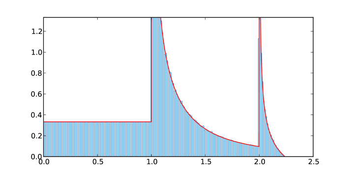
Figure 1: Simulation (blue histogram) vs explicit probability density function (red line) given by Theorem 3 for $(a,b)=(1,2)$. (Simulation used $10^{5}$ particles, each starting at the origin with a uniformly random direction, going for a total distance $1000$ each.) The plot is cutoff at $y=1.3$ since $\operatorname{pdf}_{X}(t)$ tends to infinity as $t\to 1^{+}$ and $t\to 2^{+}$.

Theorem 6.

For a box of dimension $n=3$ with side-lengths $a,b,c$, the probability density function of $X$ is given by

$$\operatorname{pdf}_{X}(t)=\dfrac{F(a,b,c,t)+F(b,c,a,t)+F(c,a,b,t)}{3\pi t^{3}(ab+ac+bc)}$$ (7)

where $F$ is the piecewise-defined function given by

$$F(a,b,c,t)=t^{3}(8a-3t)$$ (8)

for $0<t<a$, and by

$$F(a,b,c,t)=\mathopen{}\mathclose{{}\left(6t^{4}-a^{4}+6\pi a^{2}bc}\right)-4(b+c)\sqrt{\mathopen{}\mathclose{{}\left|t^{2}-a^{2}}\right|}(a^{2}+2t^{2})$$ (9)

for $a<t<\sqrt{a^{2}+b^{2}}$, and by

$$F(a,b,c,t)=6\pi a^{2}bc+b^{4}-3t^{4}-6a^{2}b^{2}+$$ (10)

$$\sqrt{\mathopen{}\mathclose{{}\left|t^{2}-a^{2}-b^{2}}\right|}4c\mathopen{}\mathclose{{}\left(a^{2}+b^{2}+2t^{2}}\right)+$$ (11)

$$+4a\sqrt{\mathopen{}\mathclose{{}\left|t^{2}-b^{2}}\right|}(b^{2}+2t^{2})-12a^{2}bc\cdot\arctan\mathopen{}\mathclose{{}\left(\dfrac{\sqrt{\mathopen{}\mathclose{{}\left|t^{2}-a^{2}-b^{2}}\right|}}{b}}\right)+$$ (12)

$$-4c\sqrt{\mathopen{}\mathclose{{}\left|t^{2}-a^{2}}\right|}(a^{2}+2t^{2})-12ab^{2}c\cdot\arctan\mathopen{}\mathclose{{}\left(\frac{\sqrt{\mathopen{}\mathclose{{}\left|t^{2}-a^{2}-b^{2}}\right|}}{a}}\right)$$ (13)

for $\sqrt{a^{2}+b^{2}}<t<\sqrt{a^{2}+b^{2}+c^{2}}.$

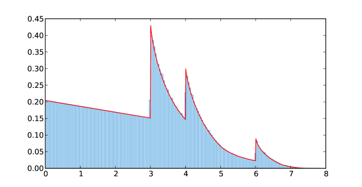
Figure 2: Simulation (blue histogram) vs explicit probability density function (red line) given by Theorem 6 for $(a,b,c)=(3,4,6)$. (Simulation used $10^{5}$ particles, each starting at the origin with a uniformly random direction, going for a total distance $1000$ each.) The fact that $\operatorname{pdf}_{X}(t)$ is not smooth at $t=5$ is barely noticeable.

Remark 14.

We note that the probability density function in Theorem 6 is analytic on all open subintervals of $(0,\sqrt{a^{2}+b^{2}+c^{2}})$ not containing any of the points

$$a,b,c,\sqrt{a^{2}+b^{2}},\sqrt{a^{2}+c^{2}},\sqrt{b^{2}+c^{2}}.$$ (15)

Moreover, it is linear on the interval $(0,\min(a,b,c))$ and has positive jump discontinuities at the points $a,b,c$. At the points $\{\sqrt{a^{2}+b^{2}},\sqrt{a^{2}+c^{2}},\sqrt{b^{2}+c^{2}}\}\setminus\{a,b,c\}$, it is continuous and differentiable.

Note that the probability distribution $X_{M,R}$ gives a larger “weight” to some particles than others, since some particles get more bounces than others for the same distance $R$. One could also consider a similar problem where we send off each particle for a certain number $N>0$ of bounces, and then consider the limit as $M\to\infty$ followed by taking the limit $N\to\infty$, where $M$ is the number of particles. This would give each particle the same “weight”. Denote the finite version of this distribution by $Y_{M,N}$ and its limit distribution as $M\to\infty$ and then $N\to\infty$ by $Y$. With regard to the previous discussion about signal loss, we call the limit distribution $X$ of $X_{M,R}$ the spreading model and we call the limit distribution of $Y_{M,N}$ the absorption model. Determining the probability density function of the absorption model appears to be the more difficult problem, and we give a formula only in dimension two:

Theorem 16.

For a box of dimension $n=2$ with side-lengths $a\leq b$, the random variable $Y_{M,N}$ converges in distribution to the random variable $Y$, as we take $M\to\infty$ followed by taking $N\to\infty$, where the probability density function $\operatorname{pdf}_{Y}(t)$ is given by

$$\frac{2}{\pi}\Bigg{(}\frac{2(a+b)}{\mathopen{}\mathclose{{}\left(a^{2}+b^{2}}\right)}-\frac{2ab}{\mathopen{}\mathclose{{}\left(a^{2}+b^{2}}\right)^{3/2}}\mathopen{}\mathclose{{}\left(\tanh^{-1}\mathopen{}\mathclose{{}\left(\frac{a}{\sqrt{a^{2}+b^{2}}}}\right)+\tanh^{-1}\mathopen{}\mathclose{{}\left(\frac{b}{\sqrt{a^{2}+b^{2}}}}\right)}\right)\Bigg{)}$$ (17)

for $0<t<a,b$, and by

$$\frac{2}{\pi}\Bigg{(}\frac{a\mathopen{}\mathclose{{}\left(b-\sqrt{t^{2}-a^{2}}}\right)}{t(b+\sqrt{t^{2}-a^{2}})\sqrt{t^{2}-a^{2}}}+\frac{2ab+2at-2a\sqrt{t^{2}-a^{2}}}{t\mathopen{}\mathclose{{}\left(a^{2}+b^{2}}\right)}+$$ (18)

$$\frac{2ab\mathopen{}\mathclose{{}\left(-\tanh^{-1}\mathopen{}\mathclose{{}\left(\frac{t}{\sqrt{a^{2}+b^{2}}}}\right)+\tanh^{-1}\mathopen{}\mathclose{{}\left(\frac{\sqrt{t^{2}-a^{2}}\sqrt{a^{2}+b^{2}}}{tb}}\right)-\tanh^{-1}\mathopen{}\mathclose{{}\left(\frac{b}{\sqrt{a^{2}+b^{2}}}}\right)}\right)}{\mathopen{}\mathclose{{}\left(a^{2}+b^{2}}\right)^{3/2}}\Bigg{)}$$ (19)

for $a<t<b$, and by

$$\frac{2}{\pi}\Bigg{(}\frac{a(b-\sqrt{t^{2}-a^{2}})}{t(b+\sqrt{t^{2}-a^{2}})\sqrt{t^{2}-a^{2}}}+\frac{b(a-\sqrt{t^{2}-b^{2}})}{t(a+\sqrt{t^{2}-b^{2}})\sqrt{t^{2}-b^{2}}}+2\frac{2ab-a\sqrt{t^{2}-a^{2}}-b\sqrt{t^{2}-b^{2}}}{t\mathopen{}\mathclose{{}\left(a^{2}+b^{2}}\right)}+$$ (20)

$$\frac{2ab\mathopen{}\mathclose{{}\left(-2\tanh^{-1}\mathopen{}\mathclose{{}\left(\frac{t}{\sqrt{a^{2}+b^{2}}}}\right)+\tanh^{-1}\mathopen{}\mathclose{{}\left(\frac{\sqrt{t^{2}-a^{2}}\sqrt{a^{2}+b^{2}}}{tb}}\right)+\tanh^{-1}\mathopen{}\mathclose{{}\left(\frac{\sqrt{t^{2}-b^{2}}\sqrt{a^{2}+b^{2}}}{ta}}\right)}\right)}{\mathopen{}\mathclose{{}\left(a^{2}+b^{2}}\right)^{3/2}}\Bigg{)}$$ (21)

for $a,b<t<\sqrt{a^{2}+b^{2}}$.

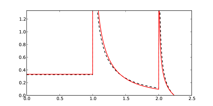
Figure 3: Probability density function for spreading model $X$ (red line) from Theorem 3 vs absorption model (black dashed line) from Theorem 16, for $(a,b)=(1,2)$.

See Figure 3 for a comparison between the probability density functions for the two different models in dimension $2$.

Remark 22.

It is not a priori obvious that the two limit distributions should differ, and it is natural to ask how much, if at all, they differ. We start by remarking that the expression for $\operatorname{pdf}_{Y}(t)$ does not simplify into the expression for $\operatorname{pdf}_{X}(t)$; indeed, for $(a,b)=(1,2)$ we have $\operatorname{pdf}_{X}(t)=1/3$ but $\operatorname{pdf}_{Y}(t)\approx 0.32553$ on the interval $(0,1)$. For very skew boxes, with $a=1$ and $b\to\infty$, it is straightforward to show that

$$\frac{\operatorname{pdf}_{Y}(b/2)}{\operatorname{pdf}_{X}(b/2)}\to\infty$$ (23)

as $b\to\infty$.

1.1 Discussion

Given a closed convex subset $C\subset{\mathbb{R}}^{n}$ with nonempty interior it is possible to define a natural probability measure on the set of lines in ${\mathbb{R}}^{n}$ that have nonempty intersection with $C$. The expected length of the intersection of a random line is then, up to a constant that only depends on $n$, given by $\operatorname{Vol}(C)/\operatorname{Area}(C)$; this is known as Santalo’s formula in the integral geometry and geometric probability literature (cf. [14, Ch. 3]).

A billiard flow on a manifold $M$ with boundary $\partial M$ gives rise to a billiard map (roughly speaking, the phase space $\Omega$ is then the collection of inward facing unit vectors $v$ at each point $x\in\partial M$). Given $(x,v)\in\Omega$ we define the associated free path as the distance the billiard particle, starting at $x$ in the direction $v$, covers before colliding with $\partial M$ again. As the billiard map carries a natural probability measure $\nu$ we can view the free path as a random variable, and the mean free path is then just its expected value. Remarkably, the mean free path (again up to a constant that only depends on the dimension) is then given by $\operatorname{Vol}(M)/\operatorname{Vol}(\partial M)$ — even for non-convex billiards. This was deduced in the seventies at the Moscow seminar on dynamical systems directed by Sinai and Alekseev but was never published and hence rederived by a number of researchers. For further details and an interesting historical survey, see Chernov’s paper [6, Sec. 2].

In spirit our methods are closely related to the ones used by Barra-Gaspard [1] in their study of the level spacing distribution for quantum graphs, and this turns out to be given by the distribution of return times to a hypersurface of section of a linear flow on a torus. In particular, for graphs with a finite number of disconnected bonds of incommensurable lengths, the hypersurface of section is the “walls” of the torus, and the level spacings of the quantum graph is exactly the same same as the free path length distribution in our setting when all particles have the same starting velocity. (In particular, compare the numerator in (37) for $v$ fixed with [1, Equation (49)].)

In [12], Marklof and Strömbergsson used the results by Barra-Gaspard to determine the gap distribution of the sequence of fractional parts of $\{\log_{b}n\}_{n\in{\mathbb{Z}}^{+}}$. The gap distribution depends on whether $b$ is trancendental, rational or algebraic; quite remarkably the density function $P(s)$ for these gaps share a number of qualitative features with the density function $\operatorname{pdf}_{X}(s)$ for free paths in our setting. Namely, the density functions both have compact support and are smooth apart from a finite number of jump discontinuities. Further, in some cases the density function is constant for $s$ small; compare Figure 1 (here $d=2$) with [12, Figure 4] (here $b=\sqrt{10}$). However, there are some important differences: for $P(s)$, left and right limits exist at the jump discontinuities, whereas for $d=2$, the right limit of $\operatorname{pdf}_{X}(s)$ is $+\infty$ at the jumps (cf. Figure 1.) Further, despite appearences, $P(s)$ is not linear near $s=0$ (cf. [12, Figure 1] corresponding to $b=e$) whereas for $d=3$, $\operatorname{pdf}_{X}(s)$ is indeed linear near $s=0$ (cf. Figure 2).

1.2 Acknowledgements

We would like to thank Z. Rudnick for some very helpful discussions, especially for suggesting the connection with integral geometry. We also thank J. Marklof for bringing references [1, 12] to our attention.

S.H. was partially supported by a grant from the Swedish Research Council (621-2011-5498). P.K. was partially supported by grants from the Göran Gustafsson Foundation for Research in Natural Sciences and Medicine, and the Swedish Research Council (621-2011-5498).

2 Proof of Theorem 1

In this section, we prove Theorem 1. For notational simplicity, we give the proof in dimension three; the general proof for $n\geq 2$ dimensions is analogous.

Given a particle with initial position $p$ and initial direction $v$, let $N_{R,p,v}$ be the number of bounce lengths we get from that particle as it has travelled a total distance $R>0$, and let $N_{R,p,v}(t)$ be the number of such bounce lengths of length at most $t\geq 0$. The uniform probability distribution on the set of bounce lengths of $M$ particles with initial positions $p^{(1)},\ldots,p^{(M)}$ and initial directions $v^{(1)},\ldots,v^{(M)}$ has the cumulative distribution function

$$\operatorname{cdf}_{X_{M,R}}(t)=\dfrac{\sum_{i=1}^{M}N_{R,p^{(i)},v^{(i)}}(t)}{\sum_{i=1}^{M}N_{R,p^{(i)},v^{(i)}}}=\dfrac{\frac{1}{M}\sum_{i=1}^{M}\dfrac{N_{R,p^{(i)},v^{(i)}}}{R}\dfrac{N_{R,p^{(i)},v^{(i)}}(t)}{N_{R,p^{(i)},v^{(i)}}}}{\frac{1}{M}\sum_{i=1}^{M}\dfrac{N_{R,p^{(i)},v^{(i)}}}{R}}.$$ (24)

(Note that the denominator is uniformly bounded from below, which follows from equation (27) below.) By the strong law of large numbers, the function (24) converges almost surely to

$$\dfrac{\int_{K}\int_{\mathbb{S}^{2}}\dfrac{N_{R,p,v}}{R}\dfrac{N_{R,p,v}(t)}{N_{R,p,v}}\mathop{dS}(v)\mathop{d\mu}(p)}{\int_{K}\int_{\mathbb{S}^{2}}\dfrac{N_{R,p,v}}{R}\mathop{dS}(v)\mathop{d\mu}(p)}$$ (25)

as $M\to\infty$, where $d\mu$ is the probability measure with which we choose the starting points, and $\mathop{dS}$ is the surface area measure on the sphere $\mathbb{S}^{2}$. By symmetry, we may restrict the inner integrals to $\mathbb{S}^{2}_{+}\mathrel{\mathop{:}}=\{(v_{x},v_{y},v_{z})\in\mathbb{S}^{2}:v_{x},v_{y},v_{z}>0\}$. We now look at the limit of (25) as $R\to\infty$, and we note that since the integrands are uniformly bounded, we may move the limit inside the integrals by the Lebesgue dominated convergence theorem. Fix one of the integrands, and denote it by $f(R,p,v,t)$. We will show that its limit $g(p,v,t)\mathrel{\mathop{:}}=\lim_{R\to\infty}f(R,p,v,t)$ exists for all $t$ and all directions $v\in\mathbb{S}^{2}$. Moreover, if $p^{(i)}$ and $v^{(i)}$ denote random variables corresponding to an initial position and an initial direction, respectively, as above, then

$$h(p^{(i)},v^{(i)},t):=\lim_{R\to\infty}\dfrac{N_{R,p^{(i)},v^{(i)}}}{R}\dfrac{N_{R,p^{(i)},v^{(i)}}(t)}{N_{R,p^{(i)},v^{(i)}}}$$ (26)

is a random variable with finite variance (and similarly for the terms in the denominator of (24); in particular recall it is uniformly bounded from below), and thus the strong law of large numbers gives that the limit of (24) as $R\to\infty$, and then $M\to\infty$ almost surely equals (25). This shows that $\lim_{M\to\infty}\lim_{R\to\infty}\operatorname{cdf}_{X_{M,R}}(t)$ exists almost surely and is equal to $\lim_{R\to\infty}\lim_{M\to\infty}\operatorname{cdf}_{X_{M,R}}(t)$.

Consider a particle with initial position $p$ and initial direction $v=(v_{x},v_{y},v_{z})\in\mathbb{S}^{2}_{+}$. By “unfolding” its motion with specular reflections on the walls of the box to the motion along a straight line in ${\mathbb{R}}^{n}$ — see Figure 4 for a 2D illustration — we see that the particle’s set of bounce lengths is identical to the set of path lengths between consecutive intersections of the straight line segment $\{p+tv:0\leq t\leq R\}$ with any of the planes $x=na,y=nb,z=nc$, $n\in{\mathbb{Z}}$. Thus we see that

$$N_{R,p,v}=R\frac{v_{x}}{a}+R\frac{v_{y}}{b}+R\frac{v_{z}}{c}+{O}(1)$$ (27)

for large $R$, and therefore

$$\dfrac{N_{R,p,v}}{R}\to\frac{v_{x}}{a}+\frac{v_{y}}{b}+\frac{v_{z}}{c}$$ (28)

as $R\to\infty$.

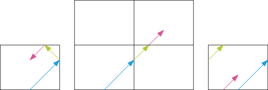
Figure 4: From left to right: Unfolding a motion with specular reflection in a 2D box to a motion the plane and then projecting back to the box.

Now project the line $\{p+tv:0\leq t\leq R\}$ to the torus ${\mathbb{R}}^{3}/\Lambda$ where $\Lambda=\{(n_{1}a,n_{2}b,n_{3}c):n_{1},n_{2},n_{3}\in{\mathbb{Z}}\}$ and let us identify the torus with the box $K$; see Figure 4. Each bounce length corresponds to a line segment which starts in one of the three planes $x=0$, $y=0$ or $z=0$ and runs in the direction $v$ to one of the three planes $x=a,y=b$ or $z=c$. There are $R\frac{v_{z}}{c}+{O}(1)$ line segments which start from the plane $z=0$, and thus the probability that a line segment starts from the plane $z=0$ is

$$\dfrac{\frac{v_{z}}{c}}{\frac{v_{x}}{a}+\frac{v_{y}}{b}+\frac{v_{z}}{c}}$$ (29)

as $R\to\infty$. By the ergodicity of the linear flow on tori (for almost all directions), the starting points of these line segments become uniformly distributed on the rectangle $[0,a]\times[0,b]\times\{0\}$ for almost all $v\in\mathbb{S}^{2}_{+}$ as $R\to\infty$; from here we will assume that $v$ is such a direction, and we will ignore the measure zero set of directions for which we do not have ergodicity. Consider one of these line segments and denote its length by $T$ and its starting point by $(x_{0},y_{0},0)$. For an arbitrary parameter $t\geq 0$, we have $T\leq t$ if and only if $tv_{x}\geq a-x_{0}$ or $tv_{y}\geq b-y_{0}$ or $tv_{x}\geq c$; the starting points $(x_{0},y_{0})\in[0,a]\times[0,b]$ which satisfy this are precisely those outside the rectangle $[0,a-tv_{x}]\times[0,b-tv_{y}]$ assuming that $tv_{z}\leq c$ and otherwise it is the whole rectangle $[0,a]\times[0,b]$. The area of that region is

$$ab-(a-tv_{x})(b-tv_{y})$$ (30)

if $a\geq tv_{x},b\geq tv_{y},c\geq tv_{z}$ and otherwise it is $ab$. Since the starting points $(x_{0},y_{0})$ are uniformly distributed in the rectangle $[0,a]\times[0,b]$ as $R\to\infty$, it follows that the probability that $T\leq t$ is

$$1-\dfrac{(a-tv_{x})(b-tv_{y})}{ab}\chi(a\geq tv_{x},b\geq tv_{y},c\geq tv_{z}),$$ (31)

where $\chi(P)$ is the indicator function which is $1$ whenever the condition $P$ is true, and $0$ otherwise. We get analogous expressions for the case when a line segment starts in the plane $x=0$ or $y=0$ instead. Thus the proportion of all line segments with length at most $t$ as $R\to\infty$ is

$$\lim_{R\to\infty}\dfrac{N_{R,p,v}(t)}{N_{R,p,v}} =\dfrac{\frac{v_{x}}{a}}{\frac{v_{x}}{a}+\frac{v_{y}}{b}+\frac{v_{z}}{c}}\mathopen{}\mathclose{{}\left(1-\dfrac{(b-tv_{y})(c-tv_{z})}{bc}\chi(a\geq tv_{x},b\geq tv_{y},c\geq tv_{z})}\right)+$$ (32)

$$\phantom{=.}\dfrac{\frac{v_{y}}{b}}{\frac{v_{x}}{a}+\frac{v_{y}}{b}+\frac{v_{z}}{c}}\mathopen{}\mathclose{{}\left(1-\dfrac{(a-tv_{x})(c-tv_{z})}{ac}\chi(a\geq tv_{x},b\geq tv_{y},c\geq tv_{z})}\right)+$$ (33)

$$\phantom{=.}\dfrac{\frac{v_{z}}{c}}{\frac{v_{x}}{a}+\frac{v_{y}}{b}+\frac{v_{z}}{c}}\mathopen{}\mathclose{{}\left(1-\dfrac{(a-tv_{x})(b-tv_{y})}{ab}\chi(a\geq tv_{x},b\geq tv_{y},c\geq tv_{z})}\right)$$ (34)

which can be written

$$1-\dfrac{\chi(a\geq tv_{x},b\geq tv_{y},c\geq tv_{z})}{abc(\frac{v_{x}}{a}+\frac{v_{y}}{b}+\frac{v_{z}}{c})}\times\\ \times\bigg{(}v_{x}(b-tv_{y})(c-tv_{z})+v_{y}(a-tv_{x})(c-tv_{z})+v_{z}(a-tv_{x})(b-tv_{y})\bigg{)}.$$ (35)

Recognizing that both integrands (28) and (35) are independent of the position $p$, we see that the limit of (25) as $R\to\infty$ may be written as

$$\lim_{R\to\infty}\lim_{M\to\infty}\operatorname{cdf}_{X_{M,R}}(t)=1-\dfrac{1}{\int_{\mathbb{S}^{2}_{+}}(v_{x}bc+av_{y}c+abv_{z})\mathop{dS}(v)}\times\\ \times\int_{\begin{subarray}{c}v\in\mathbb{S}^{2}_{+}\\ v_{x}\leq a/t\\ v_{y}\leq b/t\\ v_{z}\leq c/t\end{subarray}}((abv_{z}+av_{y}c+v_{x}bc)-2t(av_{y}v_{z}+v_{x}bv_{z}+v_{x}v_{y}c)+3t^{2}v_{x}v_{y}v_{z})\mathop{dS}(v)$$ (36)

for all $t>0$. The corresponding formula in $n$ dimensions is given by

$$\lim_{R\to\infty}\lim_{M\to\infty}\operatorname{cdf}_{X_{M,R}}(t)=1-\dfrac{\displaystyle\int_{\begin{subarray}{c}v\in\mathbb{S}^{n-1}_{+}\\ v_{i}\leq a_{i}/t\\ \text{ for }i=1,\ldots,n\end{subarray}}\mathopen{}\mathclose{{}\left(\sum_{i=1}^{n}v_{i}\prod_{j\neq i}(a_{i}-tv_{j})}\right)\mathop{dS}(v)}{\displaystyle\mathopen{}\mathclose{{}\left(\prod_{i=1}^{n}a_{i}}\right)\int_{\mathbb{S}^{n-1}_{+}}\mathopen{}\mathclose{{}\left(\sum_{i=1}^{n}\frac{v_{i}}{a_{i}}}\right)\mathop{dS}(v)}$$ (37)

for all $t>0$, where the side-lengths of the box $K$ are $a_{1},\ldots,a_{n}$ and $\mathop{dS}$ is the surface area measure on $\mathbb{S}^{n-1}_{+}\cap[0,\infty)^{n}$. (The denominator can be given explicitly by using Lemma 147 below.)

We have thus proved that the random variable $X_{M,R}$ converges in distribution to a random variable with probability density function given by (37) as we take $M\to\infty$ followed by taking $R\to\infty$, or alternatively, first taking $R\to\infty$ followed by taking $M\to\infty$. It remains to prove that this distribution agrees with the distribution of the random variable $X$ defined in the introduction.

2.1 Integral geometry

We start by recalling some standard facts from integral geometry (cf. [14, 8].) The set of directed straight lines $\ell$ in ${\mathbb{R}}^{3}$ can be parametrized by pairs $(v,q)$ where $v\in\mathbb{S}^{2}$ is a unit vector pointing in the same direction as $\ell$ and $q\in v^{\bot}$ is the unique point in $\ell$ which intersects the plane through the origin which is orthogonal to $v$. The unique translation- and rotation-invariant measure (up to a constant) on the set of directed straight lines in ${\mathbb{R}}^{3}$ is $\mathop{d\ell}\mathrel{\mathop{:}}=\mathop{dA}(q)\mathop{dS}(v)$ where $\mathop{dA}$ is the surface measure on the plane through the origin orthogonal to $v\in\mathbb{S}^{2}$, and $\mathop{dS}$ is the surface area measure on $\mathbb{S}^{2}$.

Consider the set $L_{a,b,c}$ of directed straight lines in ${\mathbb{R}}^{3}$ which intersect the box $K$. Now, since $abv_{z}+av_{y}c+v_{x}bc$ is the area of the projection of the box $K$ onto the plane $v^{\bot}$ for $v\in\mathbb{S}^{2}_{+}$, it follows that the total measure of $L_{a,b,c}$ with respect to $\mathop{d\ell}$ is

$$C_{a,b,c}\mathrel{\mathop{:}}=8\int_{\mathbb{S}^{2}_{+}}(abv_{z}+av_{y}c+v_{x}bc)\mathop{dS}(v)=2\pi(ab+ac+bc)$$ (38)

where we used symmetry, and the integral may be evaluated by switching to spherical coordinates. It follows that $\mathop{d\ell}/C_{a,b,c}$ is a probability measure on the set of directed lines intersecting the box $L_{a,b,c}$. Let $\ell$ be a random directed line with respect to this measure, and define the random variable $X\mathrel{\mathop{:}}=\operatorname{length}(\ell\cap K)$, as in the introduction. Let us determine the probability that $X\leq t$ for an arbitrary parameter $t\geq 0$. By symmetry it suffices to consider only directed lines with $v\in\mathbb{S}^{2}_{+}$. The set of all intersection points between the rectangle $[0,a]\times[0,b]\times\{0\}$ and the lines $\ell$ with $X\leq t$ and direction $v\in\mathbb{S}^{2}_{+}$ has area $ab-(a-tv_{x})(b-tv_{y})\chi(a\geq tv_{x},b\geq tv_{y},c\geq tv_{z})$, as in (30), and its projection onto the plane $v^{\bot}$ has area

$$v_{z}\mathopen{}\mathclose{{}\left[ab-(a-tv_{x})(b-tv_{y})\chi(a\geq tv_{x},b\geq tv_{y},c\geq tv_{z})}\right].$$ (39)

By symmetry it follows that the area of the set of directed lines $\ell\in L_{a,b,c}$ with $X\leq t$ and direction $v\in\mathbb{S}^{2}_{+}$ projected down to $v^{\bot}$ is

$$U(v,t) \mathrel{\mathop{:}}=v_{x}\mathopen{}\mathclose{{}\left[bc-(b-tv_{y})(c-tv_{z})\chi(a\geq tv_{x},b\geq tv_{y},c\geq tv_{z})}\right]+$$ (40)

$$\phantom{\mathrel{\mathop{:}}=.}v_{y}\mathopen{}\mathclose{{}\left[ac-(a-tv_{x})(c-tv_{z})\chi(a\geq tv_{x},b\geq tv_{y},c\geq tv_{z})}\right]+$$ (41)

$$\phantom{\mathrel{\mathop{:}}=.}v_{z}\mathopen{}\mathclose{{}\left[ab-(a-tv_{x})(b-tv_{y})\chi(a\geq tv_{x},b\geq tv_{y},c\geq tv_{z})}\right],$$ (42)

and it follows that

$$\operatorname{Prob}[X\leq t]=\dfrac{1}{C_{a,b,c}}\int_{X\leq t}\mathop{d\ell}=\dfrac{8}{C_{a,b,c}}\int_{\mathbb{S}^{2}_{+}}U(v,t)\mathop{dS}(v),$$ (43)

which we see is identical to (36), and we have thus proved that $X_{M,R}$ converges in distribution to $X$ as we take $M\to\infty$ and then $R\to\infty$. This concludes the proof of Theorem 1.

2.2 Computing the mean value

We will determine the mean value (2) of $X$; to do this we exploit the integral geometry interpretation of the random variable $X$. By symmetry it suffices to restrict to directed lines $\ell$ with $v\in\mathbb{S}^{2}_{+}$. For fixed $v\in\mathbb{S}^{2}_{+}$, denote by $Q(v)=(K+\operatorname{span}(v))\cap v^{\bot}$ the set of $q\in v^{\bot}$ such that the directed line $\ell$ parametrized by $(v,q)$ intersects $K$. We note that $X\mathop{dA}(q)$ is a volume element of the box $K$ for any fixed $v\in\mathbb{S}^{2}_{+}$, and thus integrating $X\mathop{dA}(q)$ over all $q$ yields the volume of the box. Hence the mean value is

$$\mathbb{E}\mathopen{}\mathclose{{}\left[X}\right]=\dfrac{8}{C_{a,b,c}}\int_{\mathbb{S}^{2}_{+}}\int_{Q(v)}X\mathop{dA}(q)\mathop{dS}(v)=\dfrac{8abc}{C_{a,b,c}}\int_{\mathbb{S}^{2}_{+}}\mathop{dS}(v)=\dfrac{2abc}{ab+ac+bc}.$$ (44)

In $n$ dimensions we get a normalizing factor $\frac{\operatorname{Area}(K)}{2}\cdot 2^{n}\int_{\mathbb{S}^{n-1}_{+}}v_{n}\mathop{dS}(v)$, so with the aid of the Lemma 147 in the Appendix, it follows that the mean value in $n$ dimensions is

$$\mathbb{E}\mathopen{}\mathclose{{}\left[X}\right]=\dfrac{1}{2^{n}\dfrac{1}{\pi}\dfrac{|\mathbb{S}^{n}|}{2^{n}}\frac{\operatorname{Area}(K)}{2}}2^{n}\operatorname{Vol}(K)\dfrac{|\mathbb{S}^{n-1}|}{2^{n}}=2\pi\dfrac{|\mathbb{S}^{n-1}|}{|\mathbb{S}^{n}|}\dfrac{\operatorname{Vol}(K)}{\operatorname{Area}(K)}$$ (45)

where $\operatorname{Area}(K)$ is the $(n-1)$-dimensional surface area of the box $K$, and $\operatorname{Vol}(K)$ is the volume of the box $K$.

3 Proof of Theorem 3

Using formula (37) in dimension $n=2$, we get

$$\operatorname{cdf}_{X}(t)=1-\dfrac{\displaystyle\int_{\begin{subarray}{c}v\in\mathbb{S}^{1}_{+}\\ v_{x}\leq a/t\\ v_{y}\leq b/t\end{subarray}}\mathopen{}\mathclose{{}\left(v_{x}(b-tv_{y})+v_{y}(a-tv_{x})}\right)\mathop{dS}(v)}{\displaystyle ab\int_{\mathbb{S}^{1}_{+}}\mathopen{}\mathclose{{}\left(\frac{v_{x}}{a}+\frac{v_{y}}{b}}\right)\mathop{dS}(v)}.$$ (46)

We use polar coordinates $v_{x}=\cos\theta,v_{y}=\sin\theta$ so that $\mathop{dS}(v)=\mathop{d\theta}$. Then the above becomes

$$1-\dfrac{\displaystyle\int_{\cos^{-1}(\min(a/t,1))}^{\sin^{-1}(\min(b/t,1))}\mathopen{}\mathclose{{}\left(b\cos\theta+a\sin\theta-2t\sin\theta\cos\theta}\right)\mathop{d\theta}}{\displaystyle\int_{0}^{\pi/2}\mathopen{}\mathclose{{}\left(b\cos\theta+a\sin\theta}\right)\mathop{d\theta}}=$$ (47)

$$1-\frac{1}{a+b}\mathopen{}\mathclose{{}\left[b\sin\theta-a\cos\theta+t\cos^{2}\theta}\right]_{\cos^{-1}(\min(a/t,1))}^{\sin^{-1}(\min(b/t,1))}.$$ (48)

The numerator of the second term may be written

$$\chi(b<t)\mathopen{}\mathclose{{}\left(b\cdot\frac{b}{t}-a\sqrt{1-\frac{b^{2}}{t^{2}}}+t\mathopen{}\mathclose{{}\left(1-\frac{b^{2}}{t^{2}}}\right)}\right)+\chi(b\geq t)\mathopen{}\mathclose{{}\left(b-a\cdot 0+t\cdot 0}\right)+$$ (49)

$$-\chi(a<t)\mathopen{}\mathclose{{}\left(b\sqrt{1-\frac{a^{2}}{t^{2}}}-a\cdot\frac{a}{t}+t\cdot\frac{a^{2}}{t^{2}}}\right)-\chi(a\geq t)\mathopen{}\mathclose{{}\left(b\cdot 0-a+t}\right)$$ (50)

which can be simplified to

$$\chi(b<t)\mathopen{}\mathclose{{}\left(t-b-a\sqrt{1-\frac{b^{2}}{t^{2}}}}\right)+\chi(a<t)\mathopen{}\mathclose{{}\left(t-a-b\sqrt{1-\frac{a^{2}}{t^{2}}}}\right)+\mathopen{}\mathclose{{}\left(a+b-t}\right).$$ (51)

Inserting this into (48) and differentiating yields Theorem 3.

4 Proof of Theorem 6

We will evaluate the cumulative distribution function (36) and then differentiate. The denominator of the second term of (36) is

$$\int_{\mathbb{S}^{2}_{+}}(abv_{z}+av_{y}c+v_{x}bc)\mathop{dS}(v)=\dfrac{\pi}{4}(ab+ac+bc),$$ (52)

as may be evaluated by switching to spherical coordinates. Define

$$f(a,b,c)\mathrel{\mathop{:}}=bc\int_{\begin{subarray}{c}v\in\mathbb{S}^{2}_{+}\\ v_{x}\leq a/t\\ v_{y}\leq b/t\\ v_{z}\leq c/t\end{subarray}}v_{x}\mathop{dS}(v),$$ (53)

$$g(a,b,c)\mathrel{\mathop{:}}=-2tc\int_{\begin{subarray}{c}v\in\mathbb{S}^{2}_{+}\\ v_{x}\leq a/t\\ v_{y}\leq b/t\\ v_{z}\leq c/t\end{subarray}}v_{x}v_{y}\mathop{dS}(v),$$ (54)

$$h(a,b,c)\mathrel{\mathop{:}}=3t^{2}\int_{\begin{subarray}{c}v\in\mathbb{S}^{2}_{+}\\ v_{x}\leq a/t\\ v_{y}\leq b/t\\ v_{z}\leq c/t\end{subarray}}v_{x}v_{y}v_{z}\mathop{dS}(v).$$ (55)

By symmetry, we have

$$f(c,a,b)=ab\int_{\begin{subarray}{c}v\in\mathbb{S}^{2}_{+}\\ v_{x}\leq c/t\\ v_{y}\leq a/t\\ v_{z}\leq b/t\end{subarray}}v_{x}\mathop{dS}(v)=ab\int_{\begin{subarray}{c}v\in\mathbb{S}^{2}_{+}\\ v_{x}\leq a/t\\ v_{y}\leq b/t\\ v_{z}\leq c/t\end{subarray}}v_{z}\mathop{dS}(v),$$ (56)

$$f(b,c,a)=ac\int_{\begin{subarray}{c}v\in\mathbb{S}^{2}_{+}\\ v_{x}\leq b/t\\ v_{y}\leq c/t\\ v_{z}\leq a/t\end{subarray}}v_{x}\mathop{dS}(v)=ac\int_{\begin{subarray}{c}v\in\mathbb{S}^{2}_{+}\\ v_{x}\leq a/t\\ v_{y}\leq b/t\\ v_{z}\leq c/t\end{subarray}}v_{y}\mathop{dS}(v),$$ (57)

$$g(c,a,b)=-2tb\int_{\begin{subarray}{c}v\in\mathbb{S}^{2}_{+}\\ v_{x}\leq c/t\\ v_{y}\leq a/t\\ v_{z}\leq b/t\end{subarray}}v_{x}v_{y}\mathop{dS}(v)=-2tb\int_{\begin{subarray}{c}v\in\mathbb{S}^{2}_{+}\\ v_{x}\leq a/t\\ v_{y}\leq b/t\\ v_{z}\leq c/t\end{subarray}}v_{x}v_{z}\mathop{dS}(v),$$ (58)

$$g(b,c,a)=-2ta\int_{\begin{subarray}{c}v\in\mathbb{S}^{2}_{+}\\ v_{x}\leq b/t\\ v_{y}\leq c/t\\ v_{z}\leq a/t\end{subarray}}v_{x}v_{y}\mathop{dS}(v)=-2ta\int_{\begin{subarray}{c}v\in\mathbb{S}^{2}_{+}\\ v_{x}\leq a/t\\ v_{y}\leq b/t\\ v_{z}\leq c/t\end{subarray}}v_{y}v_{z}\mathop{dS}(v),$$ (59)

and thus we can write the numerator in the second term of (36) as

$$f(a,b,c)+f(c,a,b)+f(b,c,a)+g(a,b,c)+g(c,a,b)+g(b,c,a)+h(a,b,c).$$ (60)

Exploiting the symmetries, it suffices to evaluate $h(a,b,c),g(a,b,c)$ and $f(b,c,a)$ (note the order of the arguments to $f$). We will evaluate these integrals by switching to spherical coordinates, but first we need to parametrize the part of the sphere inside the box $0\leq v_{x}\leq a/t,0\leq v_{y}\leq b/t,0\leq v_{z}\leq c/t$.

Lemma 61.

Fix $t\in(0,\sqrt{a^{2}+b^{2}+c^{2}})$. We have

$$\int_{\begin{subarray}{c}v\in\mathbb{S}^{2}_{+}\\ v_{x}\leq a/t\\ v_{y}\leq b/t\\ v_{z}\leq c/t\end{subarray}}F(v_{x},v_{y},v_{z})\mathop{dS}(v)=$$ (62)

$$\mathopen{}\mathclose{{}\left(\int_{\theta_{\text{min}}}^{\theta_{a}}\int_{0}^{\pi/2}+\int_{\theta_{a}}^{{\theta_{\text{max}}}}\int_{\varphi_{a}}^{\pi/2}-\int_{\theta_{b}}^{\theta_{\text{max}}}\int_{\varphi_{b}}^{\pi/2}}\right)\tilde{F}(\theta,\varphi)\sin\theta\mathop{d\varphi}\mathop{d\theta}$$ (63)

for any integrable function $F:\mathbb{S}^{2}_{+}\to{\mathbb{R}}$, where $\tilde{F}(\theta,\varphi)\mathrel{\mathop{:}}=F(\sin\theta\cos\varphi,\sin\theta\sin\varphi,\cos\theta)$, where

$${\theta_{\text{min}}} \mathrel{\mathop{:}}=\cos^{-1}\mathopen{}\mathclose{{}\left\{\frac{c}{t}}\right\}_{1},$$ (64)

$$\theta_{a} \mathrel{\mathop{:}}=\max({\theta_{\text{min}}},\sin^{-1}\mathopen{}\mathclose{{}\left\{\frac{a}{t}}\right\}_{1}),$$ (65)

$$\theta_{b} \mathrel{\mathop{:}}=\max({\theta_{\text{min}}},\sin^{-1}\mathopen{}\mathclose{{}\left\{\frac{b}{t}}\right\}_{1}),$$ (66)

$${\theta_{\text{max}}} \mathrel{\mathop{:}}=\sin^{-1}\mathopen{}\mathclose{{}\left\{\dfrac{\sqrt{a^{2}+b^{2}}}{t}}\right\}_{1},$$ (67)

$$\varphi_{a} \mathrel{\mathop{:}}=\cos^{-1}{\frac{a}{t\sin\theta}}\qquad(\text{whenever }a\leq t\sin\theta),$$ (68)

$$\varphi_{b} \mathrel{\mathop{:}}=\sin^{-1}{\frac{b}{t\sin\theta}}\qquad(\text{whenever }b\leq t\sin\theta).$$ (69)

and where we have used the shorthand $\mathopen{}\mathclose{{}\left\{u}\right\}_{1}\mathrel{\mathop{:}}=\min(u,1)$.

Proof.

We will parametrize the set of points $v=(v_{x},v_{y},v_{z})$ on the sphere $\mathbb{S}^{2}$ such that

$$0<v_{x}\leq a/t,$$ (70)

$$0<v_{y}\leq b/t,$$ (71)

$$0<v_{z}\leq c/t.$$ (72)

Switch to spherical coordinates $v_{x}=\sin\theta\cos\varphi,v_{y}=\sin\theta\sin\varphi,v_{z}=\cos\theta$. The non-negativity conditions of (71) are equivalent to the condition $\theta,\varphi\in(0,\pi/2)$. For such angles, the condition $v_{z}\leq c/t$ is equivalent to

$$\cos^{-1}\mathopen{}\mathclose{{}\left\{\frac{c}{t}}\right\}_{1}\leq\theta,$$ (73)

and the conditions $v_{x}\leq a/t,v_{y}\leq b/t$ are equivalent to

$$\cos^{-1}\mathopen{}\mathclose{{}\left\{\dfrac{a}{t\sin\theta}}\right\}_{1}\leq\varphi\leq\sin^{-1}\mathopen{}\mathclose{{}\left\{\dfrac{b}{t\sin\theta}}\right\}_{1}.$$ (74)

The interval (74) is non-empty for precisely those $\theta\in(0,\pi/2)$ such that $\theta\leq{\theta_{\text{max}}}$ since

$$1\leq\mathopen{}\mathclose{{}\left\{\dfrac{a}{t\sin\theta}}\right\}_{1}^{2}+\mathopen{}\mathclose{{}\left\{\dfrac{b}{t\sin\theta}}\right\}_{1}^{2}\iff 1\leq\mathopen{}\mathclose{{}\left({\dfrac{a}{t\sin\theta}}}\right)^{2}+\mathopen{}\mathclose{{}\left({\dfrac{b}{t\sin\theta}}}\right)^{2}\iff$$ (75)

$$\sin\theta\leq\dfrac{\sqrt{a^{2}+b^{2}}}{t}\iff\theta\leq\sin^{-1}\mathopen{}\mathclose{{}\left\{\dfrac{\sqrt{a^{2}+b^{2}}}{t}}\right\}_{1}.$$ (76)

Thus we may restrict $\theta$ to the interval given by the inequalities

$${\theta_{\text{min}}}\leq\theta\leq{\theta_{\text{max}}}.$$ (77)

Note that we have ${\theta_{\text{min}}}\leq{\theta_{\text{max}}}$ for all $t\leq\sqrt{a^{2}+b^{2}+c^{2}}$ since

$${\theta_{\text{min}}}\leq{\theta_{\text{max}}}\iff 1\leq\mathopen{}\mathclose{{}\left\{\frac{c}{t}}\right\}_{1}^{2}+\mathopen{}\mathclose{{}\left\{\frac{\sqrt{a^{2}+b^{2}}}{t}}\right\}_{1}^{2}\iff$$ (78)

$$1\leq\mathopen{}\mathclose{{}\left({\frac{c}{t}}}\right)^{2}+\mathopen{}\mathclose{{}\left({\frac{\sqrt{a^{2}+b^{2}}}{t}}}\right)^{2}\iff t^{2}\leq a^{2}+b^{2}+c^{2}.$$ (79)

We conclude that we can write

$$\int_{\begin{subarray}{c}v\in\mathbb{S}^{2}_{+}\\ v_{x}\leq a/t\\ v_{y}\leq b/t\\ v_{z}\leq c/t\end{subarray}}F(v_{x},v_{y},v_{z})\mathop{dS}(v)=\int_{{\theta_{\text{min}}}}^{{\theta_{\text{max}}}}\int_{\cos^{-1}\mathopen{}\mathclose{{}\left\{\frac{a}{t\sin\theta}}\right\}_{1}}^{\sin^{-1}\mathopen{}\mathclose{{}\left\{\frac{b}{t\sin\theta}}\right\}_{1}}\tilde{F}(\theta,\varphi)\sin\theta\mathop{d\varphi}\mathop{d\theta}.$$ (80)

For $\theta\in(0,\pi/2)$, note that $\cos^{-1}{\frac{a}{t\sin\theta}}$ is defined precisely when $\sin^{-1}\mathopen{}\mathclose{{}\left\{\frac{a}{t}}\right\}_{1}\leq\theta$ and that $\sin^{-1}{\frac{b}{t\sin\theta}}$ is defined precisely when $\sin^{-1}\mathopen{}\mathclose{{}\left\{\frac{b}{t}}\right\}_{1}\leq\theta$. We have ${\theta_{\text{min}}}<\theta_{a}$ if and only if $t<\sqrt{a^{2}+c^{2}}$, and we have ${\theta_{\text{min}}}<\theta_{b}$ if and only if $t<\sqrt{b^{2}+c^{2}}$. Moreover we note that we always have $\theta_{a},\theta_{b}\in[{\theta_{\text{min}}},{\theta_{\text{max}}}]$.

Let us rewrite the integration limits in the right-hand side of (80) in terms of $\varphi_{a}$ and $\varphi_{b}$. A priori, we need to distinguish between the two cases $\theta_{a}\leq\theta_{b}$ and $\theta_{b}<\theta_{a}$. If $\theta_{a}\leq\theta_{b}$ then we get

$$\mathopen{}\mathclose{{}\left(\int_{{\theta_{\text{min}}}}^{{\theta_{\text{max}}}}\int_{\cos^{-1}\mathopen{}\mathclose{{}\left\{\frac{x}{t\sin\theta}}\right\}_{1}}^{\sin^{-1}\mathopen{}\mathclose{{}\left\{\frac{y}{t\sin\theta}}\right\}_{1}}}\right)=\mathopen{}\mathclose{{}\left(\int_{\theta_{\text{min}}}^{\theta_{a}}\int_{0}^{\pi/2}+\int_{\theta_{a}}^{\theta_{b}}\int_{\varphi_{a}}^{\pi/2}+\int_{\theta_{b}}^{\theta_{\text{max}}}\int_{\varphi_{a}}^{\varphi_{b}}}\right)=$$ (81)

$$\mathopen{}\mathclose{{}\left(\int_{\theta_{\text{min}}}^{\theta_{a}}\int_{0}^{\pi/2}+\int_{\theta_{a}}^{{\theta_{\text{max}}}}\int_{\varphi_{a}}^{\pi/2}-\int_{\theta_{b}}^{{\theta_{\text{max}}}}\int_{\varphi_{a}}^{\pi/2}+\int_{\theta_{b}}^{\theta_{\text{max}}}\int_{\varphi_{a}}^{\pi/2}-\int_{\theta_{b}}^{\theta_{\text{max}}}\int_{\varphi_{b}}^{\pi/2}}\right)=$$ (82)

$$\mathopen{}\mathclose{{}\left(\int_{\theta_{\text{min}}}^{\theta_{a}}\int_{0}^{\pi/2}+\int_{\theta_{a}}^{{\theta_{\text{max}}}}\int_{\varphi_{a}}^{\pi/2}-\int_{\theta_{b}}^{\theta_{\text{max}}}\int_{\varphi_{b}}^{\pi/2}}\right).$$ (83)

If on the other hand $\theta_{b}<\theta_{a}$ then

$$\mathopen{}\mathclose{{}\left(\int_{{\theta_{\text{min}}}}^{{\theta_{\text{max}}}}\int_{\cos^{-1}\mathopen{}\mathclose{{}\left\{\frac{x}{t\sin\theta}}\right\}_{1}}^{\sin^{-1}\mathopen{}\mathclose{{}\left\{\frac{y}{t\sin\theta}}\right\}_{1}}}\right)=\mathopen{}\mathclose{{}\left(\int_{\theta_{\text{min}}}^{\theta_{b}}\int_{0}^{\pi/2}+\int_{\theta_{b}}^{\theta_{a}}\int_{0}^{\varphi_{b}}+\int_{\theta_{a}}^{\theta_{\text{max}}}\int_{\varphi_{a}}^{\varphi_{b}}}\right)=$$ (84)

$$\mathopen{}\mathclose{{}\left(\int_{\theta_{\text{min}}}^{\theta_{b}}\int_{0}^{\pi/2}+\int_{\theta_{b}}^{\theta_{a}}\int_{0}^{\pi/2}-\int_{\theta_{b}}^{\theta_{a}}\int_{\varphi_{b}}^{\pi/2}+\int_{\theta_{a}}^{\theta_{\text{max}}}\int_{\varphi_{a}}^{\pi/2}-\int_{\theta_{a}}^{\theta_{\text{max}}}\int_{\varphi_{b}}^{\pi/2}}\right)$$ (85)

which we see is identical to (83). Combining (80) and (83) we get the conclusion of the lemma. ∎

Applying Lemma 61 we get

$$h(a,b,c)=3t^{2}\int_{\begin{subarray}{c}v\in\mathbb{S}^{2}_{+}\\ v_{x}\leq a/t\\ v_{y}\leq b/t\\ v_{z}\leq c/t\end{subarray}}v_{x}v_{y}v_{z}\mathop{dS}(v)=$$ (86)

$$3t^{2}\mathopen{}\mathclose{{}\left(\int_{\theta_{\text{min}}}^{\theta_{a}}\int_{0}^{\pi/2}+\int_{\theta_{a}}^{{\theta_{\text{max}}}}\int_{\varphi_{a}}^{\pi/2}-\int_{\theta_{b}}^{\theta_{\text{max}}}\int_{\varphi_{b}}^{\pi/2}}\right)(\sin^{2}\theta\cos\theta\cos\varphi\sin\varphi)\sin\theta\mathop{d\varphi}\mathop{d\theta}.$$ (87)

An antiderivative of the integrand $\cos\varphi\sin\varphi\cdot\sin^{3}\theta\cos\theta$ with respect to $\varphi$ is $-\frac{1}{2}\cos^{2}\varphi\sin^{3}\theta\cos\theta$, and thus the above is

$$3t^{2}\mathopen{}\mathclose{{}\left(\int_{\theta_{\text{min}}}^{\theta_{a}}\mathopen{}\mathclose{{}\left.\cos^{2}\varphi}\right|_{\varphi=0}+\int_{\theta_{a}}^{{\theta_{\text{max}}}}\mathopen{}\mathclose{{}\left.\cos^{2}\varphi}\right|_{\varphi=\varphi_{a}}-\int_{\theta_{b}}^{\theta_{\text{max}}}\mathopen{}\mathclose{{}\left.\cos^{2}\varphi}\right|_{\varphi=\varphi_{b}}}\right)\frac{1}{2}\sin^{3}\theta\cos\theta\mathop{d\theta}=$$ (88)

$$3t^{2}\mathopen{}\mathclose{{}\left(\int_{\theta_{\text{min}}}^{\theta_{a}}1+\int_{\theta_{a}}^{{\theta_{\text{max}}}}\dfrac{a^{2}}{t^{2}\sin^{2}\theta}+\int_{\theta_{b}}^{\theta_{\text{max}}}\mathopen{}\mathclose{{}\left(\dfrac{b^{2}}{t^{2}\sin^{2}\theta}-1}\right)}\right)\frac{1}{2}\sin^{3}\theta\cos\theta\mathop{d\theta}=$$ (89)

$$\frac{3}{2}\mathopen{}\mathclose{{}\left(\int_{\theta_{\text{min}}}^{\theta_{a}}t^{2}\sin^{3}\theta\cos\theta\mathop{d\theta}+\int_{\theta_{a}}^{{\theta_{\text{max}}}}a^{2}\sin\theta\cos\theta\mathop{d\theta}+\int_{\theta_{b}}^{\theta_{\text{max}}}\mathopen{}\mathclose{{}\left(b^{2}\sin\theta-t^{2}\sin^{3}\theta}\right)\cos\theta\mathop{d\theta}}\right)=$$ (90)

$$\frac{3}{2}\mathopen{}\mathclose{{}\left(\mathopen{}\mathclose{{}\left[t^{2}\frac{1}{4}\sin^{4}\theta}\right]_{\theta_{\text{min}}}^{\theta_{a}}+\mathopen{}\mathclose{{}\left[a^{2}\frac{1}{2}\sin^{2}\theta}\right]_{\theta_{a}}^{{\theta_{\text{max}}}}+\mathopen{}\mathclose{{}\left[b^{2}\frac{1}{2}\sin^{2}\theta-t^{2}\frac{1}{4}\sin^{4}\theta}\right]_{\theta_{b}}^{\theta_{\text{max}}}}\right).$$ (91)

Next consider

$$g(a,b,c)=-2tc\int_{\begin{subarray}{c}v\in\mathbb{S}^{2}_{+}\\ v_{x}\leq a/t\\ v_{y}\leq b/t\\ v_{z}\leq c/t\end{subarray}}v_{x}v_{y}\mathop{dS}(v)=$$ (92)

$$-2tc\mathopen{}\mathclose{{}\left(\int_{\theta_{\text{min}}}^{\theta_{a}}\int_{0}^{\pi/2}+\int_{\theta_{a}}^{{\theta_{\text{max}}}}\int_{\varphi_{a}}^{\pi/2}-\int_{\theta_{b}}^{\theta_{\text{max}}}\int_{\varphi_{b}}^{\pi/2}}\right)(\sin^{2}\theta\cos\varphi\sin\varphi)\sin\theta\mathop{d\varphi}\mathop{d\theta}.$$ (93)

An antiderivative of the integrand $\cos\varphi\sin\varphi\cdot\sin^{3}\theta$ with respect to $\varphi$ is $-\frac{1}{2}\cos^{2}\varphi\sin^{3}\theta$, and thus the above is

$$g(a,b,c)=-2tc\int_{\begin{subarray}{c}v\in\mathbb{S}^{2}_{+}\\ v_{x}\leq a/t\\ v_{y}\leq b/t\\ v_{z}\leq c/t\end{subarray}}v_{x}v_{y}\mathop{dS}(v)=$$ (94)

$$-tc\mathopen{}\mathclose{{}\left(\int_{\theta_{\text{min}}}^{\theta_{a}}\mathopen{}\mathclose{{}\left.\cos^{2}\varphi}\right|_{\varphi=0}+\int_{\theta_{a}}^{{\theta_{\text{max}}}}\mathopen{}\mathclose{{}\left.\cos^{2}\varphi}\right|_{\varphi=\varphi_{a}}-\int_{\theta_{b}}^{\theta_{\text{max}}}\mathopen{}\mathclose{{}\left.\cos^{2}\varphi}\right|_{\varphi=\varphi_{b}}}\right)\sin^{3}\theta\mathop{d\theta}=$$ (95)

$$-tc\mathopen{}\mathclose{{}\left(\int_{\theta_{\text{min}}}^{\theta_{a}}1+\int_{\theta_{a}}^{{\theta_{\text{max}}}}\dfrac{a^{2}}{t^{2}\sin^{2}\theta}+\int_{\theta_{b}}^{\theta_{\text{max}}}\mathopen{}\mathclose{{}\left(\dfrac{b^{2}}{t^{2}\sin^{2}\theta}-1}\right)}\right)\sin^{3}\theta\mathop{d\theta}=$$ (96)

$$-tc\mathopen{}\mathclose{{}\left(\int_{\theta_{\text{min}}}^{\theta_{a}}\sin^{3}\theta\mathop{d\theta}+\int_{\theta_{a}}^{{\theta_{\text{max}}}}\dfrac{a^{2}\sin\theta}{t^{2}}\mathop{d\theta}+\int_{\theta_{b}}^{\theta_{\text{max}}}\mathopen{}\mathclose{{}\left(\dfrac{b^{2}\sin\theta}{t^{2}}-\sin^{3}\theta}\right)\mathop{d\theta}}\right)=$$ (97)

$$-tc\mathopen{}\mathclose{{}\left(\mathopen{}\mathclose{{}\left[\frac{\cos^{3}\theta}{3}-\cos\theta}\right]_{\theta_{\text{min}}}^{\theta_{a}}+\dfrac{a^{2}}{t^{2}}\mathopen{}\mathclose{{}\left[-\cos\theta}\right]_{\theta_{a}}^{{\theta_{\text{max}}}}+\mathopen{}\mathclose{{}\left[-\dfrac{b^{2}\cos\theta}{t^{2}}-\frac{\cos^{3}\theta}{3}+\cos\theta}\right]_{\theta_{b}}^{\theta_{\text{max}}}}\right).$$ (98)

We obtain $g(b,c,a)$ and $g(c,a,b)$ by switching the roles of $a,b,c$ in (98). We remark that trying to obtain $g(b,c,a)$ and $g(c,a,b)$ directly, by integrating $v_{y}v_{z}$ and $v_{x}v_{z}$, respectively, by first integrating with respect to $\varphi$, taking the limits $\varphi\to\varphi_{a}$ and $\varphi\to\varphi_{b}$, and then finding an antiderivative with respect to $\theta$, seem to result in much more complicated expressions.

Finally consider

$$f(b,c,a)=ac\int_{\begin{subarray}{c}v\in\mathbb{S}^{2}_{+}\\ v_{x}\leq a/t\\ v_{y}\leq b/t\\ v_{z}\leq c/t\end{subarray}}v_{y}\mathop{dS}(v)=$$ (99)

$$ac\mathopen{}\mathclose{{}\left(\int_{\theta_{\text{min}}}^{\theta_{a}}\int_{0}^{\pi/2}+\int_{\theta_{a}}^{{\theta_{\text{max}}}}\int_{\varphi_{a}}^{\pi/2}-\int_{\theta_{b}}^{\theta_{\text{max}}}\int_{\varphi_{b}}^{\pi/2}}\right)(\sin\theta\sin\varphi)\sin\theta\mathop{d\varphi}\mathop{d\theta}.$$ (100)

An antiderivative of the integrand $\sin\varphi\cdot\sin^{2}\theta$ with respect to $\varphi$ is $-\cos\varphi\cdot\sin^{2}\theta$, and thus the above is

$$ac\mathopen{}\mathclose{{}\left(\int_{\theta_{\text{min}}}^{\theta_{a}}\mathopen{}\mathclose{{}\left.\cos\varphi}\right|_{\varphi=0}+\int_{\theta_{a}}^{{\theta_{\text{max}}}}\mathopen{}\mathclose{{}\left.\cos\varphi}\right|_{\varphi=\varphi_{a}}-\int_{\theta_{b}}^{\theta_{\text{max}}}\mathopen{}\mathclose{{}\left.\cos\varphi}\right|_{\varphi=\varphi_{b}}}\right)\sin^{2}\theta\mathop{d\theta}=$$ (101)

$$ac\mathopen{}\mathclose{{}\left(\int_{\theta_{\text{min}}}^{\theta_{a}}1+\int_{\theta_{a}}^{{\theta_{\text{max}}}}\dfrac{a}{t\sin\theta}-\int_{\theta_{b}}^{\theta_{\text{max}}}\sqrt{1-\dfrac{b^{2}}{t^{2}\sin^{2}\theta}}}\right)\sin^{2}\theta\mathop{d\theta}=$$ (102)

$$ac\mathopen{}\mathclose{{}\left(\int_{\theta_{\text{min}}}^{\theta_{a}}\sin^{2}\theta\mathop{d\theta}+\int_{\theta_{a}}^{{\theta_{\text{max}}}}\dfrac{a\sin\theta}{t}\mathop{d\theta}-\int_{\theta_{b}}^{\theta_{\text{max}}}\sqrt{\sin^{2}\theta-\dfrac{b^{2}}{t^{2}}}\sin\theta\mathop{d\theta}}\right)=$$ (103)

$$ac\mathopen{}\mathclose{{}\left(\frac{1}{2}\mathopen{}\mathclose{{}\left[\theta-\sin\theta\cos\theta}\right]_{\theta_{\text{min}}}^{\theta_{a}}+\mathopen{}\mathclose{{}\left[\dfrac{-a\cos\theta}{t}}\right]_{\theta_{a}}^{{\theta_{\text{max}}}}-\int_{\theta_{b}}^{\theta_{\text{max}}}\sqrt{1-\dfrac{b^{2}}{t^{2}}-\cos^{2}\theta}\sin\theta\mathop{d\theta}}\right)$$ (104)

where the last integral inside the parentheses may be written as

$$\mathopen{}\mathclose{{}\left[-\frac{1}{2}\mathopen{}\mathclose{{}\left(\cos\theta\sqrt{1-\dfrac{b^{2}}{t^{2}}-\cos^{2}\theta}+\mathopen{}\mathclose{{}\left(1-\dfrac{b^{2}}{t^{2}}}\right)\tan^{-1}\mathopen{}\mathclose{{}\left(\frac{\cos\theta}{\sqrt{1-\dfrac{b^{2}}{t^{2}}-\cos^{2}\theta}}}\right)}\right)}\right]_{\theta_{b}}^{\theta_{\text{max}}}=$$ (105)

$$\mathopen{}\mathclose{{}\left[-\frac{1}{2}\mathopen{}\mathclose{{}\left(\cos\theta\sqrt{\sin^{2}\theta-\dfrac{b^{2}}{t^{2}}}+\mathopen{}\mathclose{{}\left(1-\dfrac{b^{2}}{t^{2}}}\right)\tan^{-1}\mathopen{}\mathclose{{}\left(\frac{\cos\theta}{\sqrt{\sin^{2}\theta-\dfrac{b^{2}}{t^{2}}}}}\right)}\right)}\right]_{\theta_{b}}^{\theta_{\text{max}}}$$ (106)

whenever $\theta_{b}<\pi/2$, by using the fact that $\frac{1}{2}\mathopen{}\mathclose{{}\left(x\sqrt{c-x^{2}}+c\tan^{-1}\mathopen{}\mathclose{{}\left(\frac{x}{\sqrt{c-x^{2}}}}\right)}\right)$ is an antiderivative of $\sqrt{c-x^{2}}$ with respect to $x$ when $c$ is a constant. We obtain $f(b,c,a)$ and $f(c,a,b)$ by switching the roles of $a,b,c$ in (104).

It remains to insert the limits ${\theta_{\text{min}}},\theta_{a},\theta_{b},{\theta_{\text{max}}}$ into the antiderivatives (91), (98) and (104) above. Noting that ${\theta_{\text{min}}},\theta_{a},\theta_{b},{\theta_{\text{max}}}$ are expressed in terms of piecewise-defined functions, the following manipulations will be useful. For any function $\psi$, we have

$$\psi({\theta_{\text{min}}})=\psi\mathopen{}\mathclose{{}\left(\cos^{-1}\frac{c}{t}}\right)\chi_{c}+\psi(\cos^{-1}1)(1-\chi_{c})$$ (107)

$$=\mathopen{}\mathclose{{}\left(\psi\mathopen{}\mathclose{{}\left(\cos^{-1}\frac{c}{t}}\right)-\psi(0)}\right)\chi_{c}+\psi(0)$$ (108)

where $\chi_{c}\mathrel{\mathop{:}}=\chi(t>c)$. Similarly,

$$\psi({\theta_{\text{max}}})=\mathopen{}\mathclose{{}\left(\psi\mathopen{}\mathclose{{}\left(\sin^{-1}\frac{\sqrt{a^{2}+b^{2}}}{t}}\right)-\psi(\pi/2)}\right)\chi_{a,b}+\psi(\pi/2)$$ (109)

where $\chi_{a,b}\mathrel{\mathop{:}}=\chi(\sqrt{a^{2}+b^{2}}>t)$, and

$$\psi(\theta_{a})=(1-\chi_{a})\psi(\pi/2)+(\chi_{a}-\chi_{a,c})\psi\mathopen{}\mathclose{{}\left(\sin^{-1}\frac{a}{t}}\right)+\chi_{a,c}\psi\mathopen{}\mathclose{{}\left(\cos^{-1}\frac{c}{t}}\right)$$ (110)

$$=\chi_{a,c}\cdot\mathopen{}\mathclose{{}\left(\psi\mathopen{}\mathclose{{}\left(\cos^{-1}\frac{c}{t}}\right)-\psi\mathopen{}\mathclose{{}\left(\sin^{-1}\frac{a}{t}}\right)}\right)+\chi_{a}\cdot\mathopen{}\mathclose{{}\left(\psi\mathopen{}\mathclose{{}\left(\sin^{-1}\frac{a}{t}}\right)-\psi(\pi/2)}\right)+\psi(\pi/2)$$ (111)

and similarly, $\psi(\theta_{b})$ can be written as

$$\chi_{b,c}\cdot\mathopen{}\mathclose{{}\left(\psi\mathopen{}\mathclose{{}\left(\cos^{-1}\frac{c}{t}}\right)-\psi\mathopen{}\mathclose{{}\left(\sin^{-1}\frac{b}{t}}\right)}\right)+\chi_{b}\cdot\mathopen{}\mathclose{{}\left(\psi\mathopen{}\mathclose{{}\left(\sin^{-1}\frac{b}{t}}\right)-\psi(\pi/2)}\right)+\psi(\pi/2).$$ (112)

With this we can evaluate $[\psi]_{\theta_{\text{min}}}^{\theta_{a}},[\psi]_{\theta_{a}}^{\theta_{\text{max}}},[\psi]_{\theta_{b}}^{\theta_{\text{max}}}$. But since we know that we will get a function symmetric with respect to the values $a,b,c$, it suffices to keep only those terms with $\chi_{a}$ and $\chi_{a,b}$, say, and then the other terms may be evaluated by just switching the order of $a,b,c$. Upon inserting the limits and differentiating, one obtains (after tedious calculations) that

$$\operatorname{pdf}_{X}(t)=\dfrac{F(a,b,c,t)+F(b,c,a,t)+F(c,a,b,t)}{3\pi t^{3}(ab+ac+bc)}$$ (113)

where

$$\begin{aligned} F(a,b,c,t)\mathrel{\mathop{:}}=\ &(8at^{3}-3t^{4})+\\ \chi(t\geq a)\Bigg{(}\mathopen{}\mathclose{{}\left(6t^{4}-a^{4}+6\pi a^{2}bc}\right)-&(8at^{3}-3t^{4})-4(b+c)\sqrt{\mathopen{}\mathclose{{}\left|t^{2}-a^{2}}\right|}(a^{2}+2t^{2})\Bigg{)}+\end{aligned}$$ (114)

$$\begin{aligned} \chi(t\geq\sqrt{a^{2}+b^{2}})\Bigg{[}&a^{4}+b^{4}-9t^{4}-6a^{2}b^{2}+\sqrt{\mathopen{}\mathclose{{}\left|t^{2}-a^{2}-b^{2}}\right|}4c\mathopen{}\mathclose{{}\left(a^{2}+b^{2}+2t^{2}}\right)+\\ &4a\sqrt{\mathopen{}\mathclose{{}\left|t^{2}-b^{2}}\right|}(b^{2}+2t^{2})-12a^{2}bc\cdot\arctan\mathopen{}\mathclose{{}\left(\dfrac{\sqrt{\mathopen{}\mathclose{{}\left|t^{2}-a^{2}-b^{2}}\right|}}{b}}\right)+\\ &4b\sqrt{\mathopen{}\mathclose{{}\left|t^{2}-a^{2}}\right|}(a^{2}+2t^{2})-12ab^{2}c\cdot\arctan\mathopen{}\mathclose{{}\left(\frac{\sqrt{\mathopen{}\mathclose{{}\left|t^{2}-a^{2}-b^{2}}\right|}}{a}}\right)\Bigg{]}.\end{aligned}$$ (115)

Rewriting $F$ as a piecewise function, we get Theorem (6).

5 Proof of Theorem 16

Consider the distribution of the random variable $Y_{M,N}$. Since we record the same number of bounces for each choice of angle $\varphi$ we may replace the $M$-particle system with a one particle system $Y_{N}$ as follows: randomly select, with uniform distribution, the angle $\varphi$ and generate $N$ bounce lengths and randomly select one of these bounce lengths (with uniform distribution); by the strong law of large numbers, $Y_{M,N}$ converges in distribution to $Y_{N}$ as $M\to\infty$.

We now determine the limit distribution of $Y_{N}$. As before, we first unfold the motion, and replace motion in a box with specular reflections on the walls with motion in ${\mathbb{R}}^{2}$; see Figure 4. The path lengths between bounces is then the same as the lengths between the intersections with horizontal or vertical grid lines. To understand the spatial distribution, we project the dynamics to the torus ${\mathbb{R}}^{2}/\Lambda$ where $\Lambda$ is the lattice

$$\Lambda=\{(n_{1}a,n_{2}b):n_{1},n_{2}\in{\mathbb{Z}}\},$$ (116)

and we may identify the torus with the rectangle $[0,a]\times[0,b]$.

Let us first consider the motion of a single particle with an arbitrary initial position, and direction of motion given by an angle $\varphi$. Taking symmetries into account, we may assume that $\varphi\in[0,\pi/2]$. (Note that $\frac{d\varphi}{\pi/2}$ gives a probability measure on these angles.) If the particle travels a large distance $R>0$, the number of intersections with horizontal, respectively vertical, grid lines is $\frac{R\sin\varphi}{b}+O(1)$, respectively $\frac{R\cos\varphi}{a}+O(1)$. Thus, in the limit $R\to\infty$, the probability of a line segment beginning at a horizontal (respectively vertical) grid line is given by $P_{h}$, respectively $P_{v}$ (here we suppress the dependence on $\varphi$) where

$$P_{h}\mathrel{\mathop{:}}=\frac{\frac{\sin\varphi}{b}}{\frac{\sin\varphi}{b}+\frac{\cos\varphi}{a}},\quad P_{v}\mathrel{\mathop{:}}=\frac{\frac{\cos\varphi}{a}}{\frac{\sin\varphi}{b}+\frac{\cos\varphi}{a}}.$$ (117)

The unfolded flow on the torus is ergodic for almost all $\varphi$, and thus the starting points of the line segments becomes uniformly distributed as $R\to\infty$ for almost all $\varphi$.

Let

$$T=T(\varphi)\mathrel{\mathop{:}}=a/\cos\varphi.$$ (118)

Since $\sin\varphi=\sqrt{T^{2}-a^{2}}/T$, we obtain that

$$P_{h}=\frac{\sqrt{T^{2}-a^{2}}}{b+\sqrt{T^{2}-a^{2}}},\quad P_{v}=\frac{b}{b+\sqrt{T^{2}-a^{2}}}.$$ (119)

Let $\theta=\arctan b/a$ denote the angle of the diagonal in the box, and assume that $0\leq\varphi\leq\theta$. We then observe the following regarding the line segment lengths.

First, if the segment begins at a horizontal line, it must end at a vertical line, and the possible lengths of these segment lie between $0$ and $T$. We find that these lengths are uniformly distributed in $[0,T]$ since the starting points of the segments are uniformly distributed.

On the other hand, if the line segment begins at a vertical line, it can either end at a vertical or horizontal line. Since the starting points are uniformly distributed, the former happens with probability

$$\frac{a\tan\varphi}{b}=\frac{a\frac{\sqrt{T^{2}-a^{2}}}{a}}{b}=\frac{\sqrt{T^{2}-a^{2}}}{b}$$ (120)

and the length of the segment is again uniformly distributed in $[0,T]$, whereas the latter happens with probability

$$\frac{b-a\tan\varphi}{b}=1-\frac{\sqrt{T^{2}-a^{2}}}{b}$$ (121)

in which case the segment is always of length $T$.

Now, $\varphi\in[0,\theta]$ implies that $T\in[a,\sqrt{a^{2}+b^{2}}]$, and noting that

$$\frac{d\varphi}{\mathop{dT}}=\frac{a}{T\sqrt{T^{2}-a^{2}}}$$ (122)

we find that the probability of observing a line segment of length $t$ is the sum of a “singular part” (the segment begins and ends on vertical lines; note that all such segments have the same lengths) and a “smooth part” (the segment does not begin and end on vertical lines). Moreover, the smooth part contribution equals

$$\frac{1}{\pi/2}\int_{\max(a,t)}^{\sqrt{a^{2}+b^{2}}}\frac{1}{T}\mathopen{}\mathclose{{}\left(P_{h}+P_{v}\frac{a\tan\varphi}{b}}\right)\frac{d\varphi}{\mathop{dT}}\mathop{dT}$$ (123)

which, on inserting (119), equals

$$\frac{1}{\pi/2}\int_{\max(a,t)}^{\sqrt{a^{2}+b^{2}}}\frac{1}{T}\cdot\mathopen{}\mathclose{{}\left(\frac{\sqrt{T^{2}-a^{2}}}{b+\sqrt{T^{2}-a^{2}}}+\frac{b}{b+\sqrt{T^{2}-a^{2}}}\frac{a\tan\varphi}{b}}\right)\cdot\frac{a}{T\sqrt{T^{2}-a^{2}}}\mathop{dT}=$$ (124)

$$\frac{1}{\pi/2}\int_{\max(a,t)}^{\sqrt{a^{2}+b^{2}}}\frac{1}{T}\cdot\mathopen{}\mathclose{{}\left(\frac{\sqrt{T^{2}-a^{2}}}{b+\sqrt{T^{2}-a^{2}}}+\frac{b}{b+\sqrt{T^{2}-a^{2}}}\frac{\sqrt{T^{2}-a^{2}}}{b}}\right)\cdot\frac{a}{T\sqrt{T^{2}-a^{2}}}\mathop{dT}=$$ (125)

$$\frac{1}{\pi/2}\int_{\max(a,t)}^{\sqrt{a^{2}+b^{2}}}\frac{2a}{b+\sqrt{T^{2}-a^{2}}}\cdot\frac{\mathop{dT}}{T^{2}}.$$ (126)

On the other hand, the “singular part contribution”, provided $t\geq a$, to the probability of a segment having length $t$ equals

$$\frac{P_{v}}{\pi/2}\cdot\frac{b-a\tan\varphi}{b}\cdot\frac{d\varphi}{dt}=\frac{1}{\pi/2}\cdot\frac{b}{b+\sqrt{t^{2}-a^{2}}}\cdot\mathopen{}\mathclose{{}\left(1-\frac{\sqrt{t^{2}-a^{2}}}{b}}\right)\cdot\frac{a}{t\sqrt{t^{2}-a^{2}}}=$$ (127)

$$\frac{1}{\pi/2}\cdot\frac{a}{t(b+\sqrt{t^{2}-a^{2}})\sqrt{t^{2}-a^{2}}}\cdot\mathopen{}\mathclose{{}\left(b-\sqrt{t^{2}-a^{2}}}\right).$$ (128)

In case $\theta\leq\varphi\leq\pi/2$, a similar argument (we simple reverse the roles of $a$ and $b$) shows that the smooth contribution equals

$$\frac{1}{\pi/2}\int_{\max(b,t)}^{\sqrt{a^{2}+b^{2}}}\frac{2b}{a+\sqrt{T^{2}-b^{2}}}\cdot\frac{\mathop{dT}}{T^{2}}$$ (129)

and that the singular contribution (if $t\geq b$) equals

$$\frac{1}{\pi/2}\cdot\frac{b}{t(a+\sqrt{t^{2}-b^{2}})\sqrt{t^{2}-b^{2}}}\cdot\mathopen{}\mathclose{{}\left(a-\sqrt{t^{2}-b^{2}}}\right).$$ (130)

Thus, if we let $P_{\operatorname{sing}}(t)$ denote the “singular contribution” to the probability density function we find the following: if $t<a$, then

$$P_{\operatorname{sing}}(t)=0$$ (131)

if $t\in[a,b]$, then

$$P_{\operatorname{sing}}(t)=\frac{1}{\pi/2}\cdot\frac{a\mathopen{}\mathclose{{}\left(b-\sqrt{t^{2}-a^{2}}}\right)}{t(b+\sqrt{t^{2}-a^{2}})\sqrt{t^{2}-a^{2}}}$$ (132)

and if $t\in[b,\sqrt{a^{2}+b^{2}}]$, then

$$P_{\operatorname{sing}}(t)=\frac{1}{\pi/2}\cdot\mathopen{}\mathclose{{}\left(\frac{a(b-\sqrt{t^{2}-a^{2}})}{t(b+\sqrt{t^{2}-a^{2}})\sqrt{t^{2}-a^{2}}}+\frac{b(a-\sqrt{t^{2}-b^{2}})}{t(a+\sqrt{t^{2}-b^{2}})\sqrt{t^{2}-b^{2}}}}\right).$$ (133)

Remark 134.

Note that $P_{\operatorname{sing}}$ has a singularity of type $(t-a)^{-1/2}$ just to the right of $t=a$ (and similarly just to the right of $t=b$). In a sense this singularity arises from the singularity in the change of variables $\varphi\mapsto T$ since $\frac{d\varphi}{dT}=\frac{a}{T\sqrt{T^{2}-a^{2}}}$. The reason for the singularities in the spreading model for $n=2$ is similar, as the spreading model can be obtained from the absorption model by a smooth change of the angular measure.

Similarly, the “smooth part” of the contribution is (for $t\in[0,\sqrt{a^{2}+b^{2}}]$) given by

$$P_{\operatorname{smooth}}(t)=\frac{1}{\pi/2}\mathopen{}\mathclose{{}\left(\int_{\max(a,t)}^{\sqrt{a^{2}+b^{2}}}\frac{2a}{b+\sqrt{T^{2}-a^{2}}}\cdot\frac{\mathop{dT}}{T^{2}}+\int_{\max(b,t)}^{\sqrt{a^{2}+b^{2}}}\frac{2b}{a+\sqrt{T^{2}-b^{2}}}\cdot\frac{\mathop{dT}}{T^{2}}}\right)$$ (135)

Hence the probability density function of the distribution of the segment length $t$ is given by

$$\operatorname{pdf}_{Y}(t)=P_{\operatorname{sing}}(t)+P_{\operatorname{smooth}}(t).$$ (136)

We will now evaluate $P_{\operatorname{smooth}}(t)$. An antiderivative of $\frac{2a}{b+\sqrt{T^{2}-a^{2}}}\cdot\frac{1}{T^{2}}$ with respect to $T$ for $T\in(a,\sqrt{a^{2}+b^{2}})$ is

$$\frac{2a(\sqrt{T^{2}-a^{2}}-b)}{T\mathopen{}\mathclose{{}\left(a^{2}+b^{2}}\right)}+\frac{2ab\mathopen{}\mathclose{{}\left(\tanh^{-1}\mathopen{}\mathclose{{}\left(\frac{T}{\sqrt{a^{2}+b^{2}}}}\right)-\tanh^{-1}\mathopen{}\mathclose{{}\left(\frac{\sqrt{T^{2}-a^{2}}\sqrt{a^{2}+b^{2}}}{Tb}}\right)}\right)}{\mathopen{}\mathclose{{}\left(a^{2}+b^{2}}\right)^{3/2}}$$ (137)

where $\tanh^{-1}(z)=\frac{1}{2}\log\frac{1+z}{1-z}$ for $\mathopen{}\mathclose{{}\left|z}\right|<1$. (A quick calculation shows that $\frac{\sqrt{T^{2}-a^{2}}\sqrt{a^{2}+b^{2}}}{Tb}<1$ whenever $a<T<\sqrt{a^{2}+b^{2}}$.) We can rewrite (137) as

$$\frac{2a(\sqrt{T^{2}-a^{2}}-b)}{T\mathopen{}\mathclose{{}\left(a^{2}+b^{2}}\right)}+\frac{ab\log\mathopen{}\mathclose{{}\left(\frac{\mathopen{}\mathclose{{}\left(\sqrt{a^{2}+b^{2}}+T}\right)\mathopen{}\mathclose{{}\left(Tb-\sqrt{T^{2}-a^{2}}\sqrt{a^{2}+b^{2}}}\right)}{\mathopen{}\mathclose{{}\left(\sqrt{a^{2}+b^{2}}-T}\right)\mathopen{}\mathclose{{}\left(Tb+\sqrt{T^{2}-a^{2}}\sqrt{a^{2}+b^{2}}}\right)}}\right)}{\mathopen{}\mathclose{{}\left(a^{2}+b^{2}}\right)^{3/2}}$$ (138)

By l’Hôpital’s rule we have

$$\lim_{T\to\sqrt{a^{2}+b^{2}}+}\frac{Tb-\sqrt{T^{2}-a^{2}}\sqrt{a^{2}+b^{2}}}{\sqrt{a^{2}+b^{2}}-T}=\lim_{T\to\sqrt{a^{2}+b^{2}}+}\frac{b-\frac{T}{\sqrt{T^{2}-a^{2}}}\sqrt{a^{2}+b^{2}}}{-1}=\frac{a^{2}}{b}$$ (139)

so the limit of (137) as $T\to\sqrt{a^{2}+b^{2}}+$ is

$$\frac{ab\log\mathopen{}\mathclose{{}\left(\mathopen{}\mathclose{{}\left(\frac{a^{2}}{b}}\right)\cdot\frac{\mathopen{}\mathclose{{}\left(\sqrt{a^{2}+b^{2}}+\sqrt{a^{2}+b^{2}}}\right)}{\mathopen{}\mathclose{{}\left(b\sqrt{a^{2}+b^{2}}+b\sqrt{a^{2}+b^{2}}}\right)}}\right)}{\mathopen{}\mathclose{{}\left(a^{2}+b^{2}}\right)^{3/2}}=\frac{2ab\log\mathopen{}\mathclose{{}\left(\frac{a}{b}}\right)}{\mathopen{}\mathclose{{}\left(a^{2}+b^{2}}\right)^{3/2}}.$$ (140)

The limit of (137) as $T\to a+$ is

$$\frac{-2b}{\mathopen{}\mathclose{{}\left(a^{2}+b^{2}}\right)}+\frac{2ab\tanh^{-1}\mathopen{}\mathclose{{}\left(\frac{a}{\sqrt{a^{2}+b^{2}}}}\right)}{\mathopen{}\mathclose{{}\left(a^{2}+b^{2}}\right)^{3/2}}.$$ (141)

Thus, assuming $a<b$, we can write $\frac{\pi}{2}P_{\operatorname{smooth}}(t)$ as

$$\frac{2(a+b)}{\mathopen{}\mathclose{{}\left(a^{2}+b^{2}}\right)}-\frac{2ab}{\mathopen{}\mathclose{{}\left(a^{2}+b^{2}}\right)^{3/2}}\mathopen{}\mathclose{{}\left(\tanh^{-1}\mathopen{}\mathclose{{}\left(\frac{a}{\sqrt{a^{2}+b^{2}}}}\right)+\tanh^{-1}\mathopen{}\mathclose{{}\left(\frac{b}{\sqrt{a^{2}+b^{2}}}}\right)}\right)$$ (142)

if $t<a,b$, or as

$$\frac{2ab+2at-2a\sqrt{t^{2}-a^{2}}}{t\mathopen{}\mathclose{{}\left(a^{2}+b^{2}}\right)}+$$ (143)

$$\frac{2ab\mathopen{}\mathclose{{}\left(-\tanh^{-1}\mathopen{}\mathclose{{}\left(\frac{t}{\sqrt{a^{2}+b^{2}}}}\right)+\tanh^{-1}\mathopen{}\mathclose{{}\left(\frac{\sqrt{t^{2}-a^{2}}\sqrt{a^{2}+b^{2}}}{tb}}\right)-\tanh^{-1}\mathopen{}\mathclose{{}\left(\frac{b}{\sqrt{a^{2}+b^{2}}}}\right)}\right)}{\mathopen{}\mathclose{{}\left(a^{2}+b^{2}}\right)^{3/2}}$$ (144)

if $a<t<b$ or as

$$2\frac{2ab-a\sqrt{t^{2}-a^{2}}-b\sqrt{t^{2}-b^{2}}}{t\mathopen{}\mathclose{{}\left(a^{2}+b^{2}}\right)}+$$ (145)

$$\frac{2ab\mathopen{}\mathclose{{}\left(-2\tanh^{-1}\mathopen{}\mathclose{{}\left(\frac{t}{\sqrt{a^{2}+b^{2}}}}\right)+\tanh^{-1}\mathopen{}\mathclose{{}\left(\frac{\sqrt{t^{2}-a^{2}}\sqrt{a^{2}+b^{2}}}{tb}}\right)+\tanh^{-1}\mathopen{}\mathclose{{}\left(\frac{\sqrt{t^{2}-b^{2}}\sqrt{a^{2}+b^{2}}}{ta}}\right)}\right)}{\mathopen{}\mathclose{{}\left(a^{2}+b^{2}}\right)^{3/2}}$$ (146)

if $a,b<t$. Adding $P_{\operatorname{sing}}(t)$ to this, we get Theorem 16.

Appendix A Calculation of an integral

Lemma 147.

Write $|\mathbb{S}^{n-1}|$ for the $(n-1)$-dimensional surface area of the sphere $\mathbb{S}^{n-1}\subseteq{\mathbb{R}}^{n}$. Then we have

$$\int_{\mathbb{S}^{n-1}_{+}}v_{n}\mathop{dS}(v)=\dfrac{1}{\pi}\dfrac{|\mathbb{S}^{n}|}{2^{n}}.$$ (148)

where $\mathbb{S}^{n-1}_{+}\mathrel{\mathop{:}}=\mathbb{S}^{n-1}\cap(0,\infty)^{n}$ is the part of the sphere $\mathbb{S}^{n-1}$ with positive coordinates.

Proof.

We may parametrize $v=(v_{1},\ldots,v_{n})\in\mathbb{S}^{n-1}_{+}$ with

$$v_{1} =\cos\theta_{1}$$ (149)

$$v_{2} =\sin\theta_{1}\cos\theta_{2}$$ (150)

$$v_{3} =\sin\theta_{1}\sin\theta_{2}\cos\theta_{3}$$ (151)

$$\vdots$$ (152)

$$v_{n-1} =\sin\theta_{1}\cdots\sin\theta_{n-2}\cos\theta_{n-1}$$ (153)

$$v_{n} =\sin\theta_{1}\cdots\sin\theta_{n-2}\sin\theta_{n-1}$$ (154)

for $\theta_{1},\ldots,\theta_{n-1}\in(0,\pi/2)$. We have the spherical area element

$$\mathop{dS}(v)=\sin^{n-2}\theta_{1}\sin^{n-3}\theta_{2}\cdots\sin\theta_{n-2}\mathop{d\theta_{1}}\cdots\mathop{d\theta_{n-1}}.$$ (155)

Thus we get

$$\int_{\mathbb{S}^{n-1}_{+}}v_{n}\mathop{dS}(v)=\prod_{i=1}^{n-1}\int_{0}^{\pi/2}\sin^{n-1-i}\theta_{i}\mathop{d\theta_{i}}.$$ (156)

Introducing an additional integration variable $\theta_{n}$, we recognize the integrand as the spherical area element in $n+1$ dimensions, and thus the above is

$$\dfrac{1}{\int_{0}^{\pi/2}\mathop{d\theta_{n}}}\prod_{i=1}^{n}\int_{0}^{\pi/2}\sin^{n-1-i}\theta_{i}\mathop{d\theta_{i}}=\dfrac{1}{\pi/2}\dfrac{|\mathbb{S}^{n}|}{2^{n+1}}.$$ (157)

since $\int_{\mathbb{S}^{n}_{+}}\mathop{dS}(v)=|\mathbb{S}^{n}|/2^{n+1}$. ∎

References

[1]
F. Barra and P. Gaspard.
On the level spacing distribution in quantum graphs.
J. Statist. Phys., 101(1-2):283–319, 2000.
[2]
C. Boldrighini, L. A. Bunimovich, and Y. G. Sinaĭ.
On the Boltzmann equation for the Lorentz gas.
J. Statist. Phys., 32(3):477–501, 1983.
[3]
J. Bourgain, F. Golse, and B. Wennberg.
On the distribution of free path lengths for the periodic Lorentz
gas.
Comm. Math. Phys., 190(3):491–508, 1998.
[4]
L. A. Bunimovich and Y. G. Sinaĭ.
Statistical properties of Lorentz gas with periodic configuration
of scatterers.
Comm. Math. Phys., 78(4):479–497, 1980/81.
[5] M. Bäckström, S. Holmin, P. Kurlberg, D. Månsson. Randomized Ray Tracing for Modeling UWB Transients in a Reverberation Chamber. In preparation.
[6]
N. Chernov.
Entropy, Lyapunov exponents, and mean free path for billiards.
J. Statist. Phys., 88(1-2):1–29, 1997.
[7]
F. Golse and B. Wennberg.
On the distribution of free path lengths for the periodic Lorentz
gas. II.
M2AN Math. Model. Numer. Anal., 34(6):1151–1163, 2000.
[8]
D. A. Klain and G.-C. Rota.
Introduction to geometric probability.
Lezioni Lincee. [Lincei Lectures]. Cambridge University Press,
Cambridge, 1997.
[9]
D. Månsson, personal communication.
[10]
J. Marklof and A. Strömbergsson.
The distribution of free path lengths in the periodic Lorentz gas
and related lattice point problems.
Ann. of Math. (2), 172(3):1949–2033, 2010.
[11]
J. Marklof and A. Strömbergsson.
The Boltzmann-Grad limit of the periodic Lorentz gas.
Ann. of Math. (2), 174(1):225–298, 2011.
[12]
J. Marklof and A. Strömbergsson.
Gaps between logs.
Bull. Lond. Math. Soc., 45(6):1267–1280, 2013.
[13]
J. Marklof and A. Strömbergsson.
Free path lengths in quasicrystals.
Comm. Math. Phys., 330(2):723–755, 2014.
[14]
L. A. Santaló.
Integral geometry and geometric probability.
Cambridge Mathematical Library. Cambridge University Press,
Cambridge, second edition, 2004.
With a foreword by Mark Kac.
[15]
H. Spohn.
The Lorentz process converges to a random flight process.
Comm. Math. Phys., 60(3):277–290, 1978.
[16]
B. Wennberg.
Free path lengths in quasi crystals.
J. Stat. Phys., 147(5):981–990, 2012.