Spatiotemporal algebraically localized waveforms for a nonlinear Schrödinger model with gain and loss

Abstract

We consider the asymptotic behavior of the solutions of a nonlinear Schrödinger (NLS) model incorporating linear and nonlinear gain/loss. First, we describe analytically the dynamical regimes (depending on the gain/loss strengths), for finite-time collapse, decay, and global existence of solutions in the dynamics. Then, for all the above parametric regimes, we use direct numerical simulations to study the dynamics corresponding to algebraically decaying initial data. We identify crucial differences between the dynamics of vanishing initial conditions, and those converging to a finite constant background: in the former (latter) case we find strong (weak) collapse or decay, when the gain/loss parameters are selected from the relevant regimes. One of our main results, is that in all the above regimes, non-vanishing initial data transition through spatiotemporal, algebraically decaying waveforms. While the system is nonintegrable, the evolution of these waveforms is reminiscent to the evolution of the Peregrine rogue wave of the integrable NLS limit. The parametric range of gain and loss for which this phenomenology persists is also touched upon.

I Introduction

In the present paper, we investigate the dynamics of the following nonlinear Schrödinger (NLS) model:

$$\!\!\!\!\!\!\!\!\!{\rm i}\partial_{t}u+\frac{1}{2}\partial_{x}^{2}u+|u|^{2}u = {\rm i}\gamma u+{\rm i}\delta|u|^{2}u,\quad x\in\mathbb{R},\quad t\in[0,T_{\mathrm{max}}).$$ (1)

Here, $u(x,t)$ is the unknown complex field, subscripts denote partial derivatives, and constants $\gamma,\leavevmode\nobreak\ \delta\in\mathbb{R}$ describe gain or loss (see below). We supplement Eq. (1) with the periodic boundary conditions for $u$:

$$u(x+2L,t)=u(x,t),$$ (2)

for given $L>0$, and with the initial condition

$$u(x,0)=u_{0}(x),$$ (3)

also satisfying the periodicity conditions (2).

Equation (1) is one of the most fundamental NLS models incorporating linear and nonlinear gain/loss effects. In particular, the parameter $\gamma$ describes linear loss ($\gamma<0$) [or gain ($\gamma>0$)], while $\delta$ describes nonlinear gain ($\delta>0$) [or loss ($\delta<0$)]. The presence of these effects is physically relevant in the context of nonlinear optics Hasegawa & Kodama (1996); Agrawal (2003); Kivshar & Agrawal (2003); akbook ; Gagnon : in this context, $\gamma$ describes a linear absorption ($\gamma<0$) [or linear amplification ($\gamma>0$)], while $\delta$ stands for nonlinear amplification ($\delta>0$) [or gain saturation-two photon absorption ($\delta<0$)]. Generally, for physically relevant settings, such terms play a crucial role in the stability of solitons potentially rendering them attractors for the dynamics. Note that the integrable limit of $\gamma=\delta=0$, i.e., the conservative NLS equation, possesses soliton solutions; in the case of the self-focusing nonlinearity considered herein, there exist bright soliton solutions that decay to zero at infinity.

Apart from bright solitons, and again in the integrable version of Eq. (1), there exists still another important class of solutions: a rational solution, namely the Peregrine rogue wave (PRW), as well as space- or time-periodic solutions, referred to as the Akhmediev and Kuznetsov-Ma (KMb) breathers, respectively. These solutions have emerged from the seminal works of Peregrine H_Peregrine , Kuznetsov kuz , Ma ma , and Akhmediev akh , as well as Dysthe and Trulsen dt . In recent years, the aforementioned wave structures are receiving increasing attention, due to their argued potential relevance towards the mathematical description of extreme events and rogue waves k2a ; k2b ; k2c ; k2d . The interest in these solutions is justified by many relevant experimental observations in various physical contexts, ranging from hydrodynamics hydro ; hydro2 ; hydro3 and nonlinear optics opt1 ; opt2 ; opt3 ; opt4 ; opt5 ; laser , to superfluidity He and plasmas plasma .

An important question concerns the robustness of rational solutions in the presence of integrable and non-integrable perturbations. In selected special cases it was found devine ; NR4Anki ; NR5Wang ; NRbor6 ; NRbor5a , that rational solutions can still be identified, in Hirota-type variants of the original NLS equation (see also Ref. calinibook for relevant work in higher-order NLS models). However, in broader classes of non-integrable perturbed NLS models, this remains a significant open problem.

Another approach towards exploring the robustness of these excitations relies on the connection with the KMb state. The latter, is periodic in the evolution variable and, in the limit of infinite period, reduces to the PRW. The dynamical robustness of KMb against dispersive or diffusive, higher-order perturbations was studied by means of a perturbed inverse scattering transform approach KalimerisGarnier . In the latter work, it was shown that KMb is rather robust against dispersive perturbations, but it is strongly affected by dissipative ones. In another related recent work KMS , a Floquet stability analysis of the KMb was performed in the integrable NLS, attempting –via the approach to the infinite period limit– to shed light to the stability features of the PRW state.

More relevant to our concerns in the present work, are recent contributions studying the role of driving and linear loss. Reference onorato1 , for instance (see also references therein), investigates the effect of wind and dissipation on the nonlinear stages of the modulational instability (MI) in the context of water waves ZO . Further extensions considering the case of strong wind (whose effect is of the same order as the wave steepness), are given in Ref. brunetti . This approach, allows for the construction of approximate rational solutions for the considered model. The effects of slow/strong linear forcing in the statistics of extreme events, were also studied EPeli . It was highlighted therein, that when the forcing is short in time and effectively strong, it facilitates the occurrence of extreme wave conditions. At this point, it is important to note that the MI of background plane waves (which host the rational solutions), may lead to homoclinic-type solutions, which can also considered as candidates for rogue waves calini2012 . Such phenomena have been observed and analyzed in a variety of extended NLS models, that incorporate higher-order dissipative or dispersive effects (pertinent studies also include the Dysthe model NR11 ).

In this work, we aim to examine a rather different question, related to the PRW. In particular, its algebraic spatiotemporal localization, motivates us to study the dynamics of Eq. (1) for initial data with an algebraic decay rate. Our plan is as follows. First, we identify analytically the regimes defined by the gain/loss parameters where the solutions may exhibit finite time collapse, vanishing decay, or nontrivial (non-decaying) dynamics. The latter are captured by an attracting set for all initial conditions in the infinite dimensional space. Then, we proceed to examine, by means of direct numerical simulations, the evolution of algebraically decaying initial data in the prescribed dynamical regimes. Our main findings are summarized below.

To begin, crucial differences are detected between the dynamics corresponding to asymptotically vanishing or non-vanishing initial data. For vanishing initial conditions, we observe the strong collapse/decay of the resulting waveforms Babis . The collapse is manifested by the local increase of amplitude which grows towards the singularity, while decay is manifested by a flattening, leading towards convergence to the trivial state. On the other hand, nonvanishing initial conditions exhibit a weak type of collapse/decay. In weak collapse, as time progresses, a fraction of the wave approaches the singularity with long tails left behind. In our case, these tails consist of a multi-hump, non-collapsing wave-train of solitonic structures, occupying a finite spatial interval of increasing length as time increases. Collapse occurs through time-oscillations of increasing amplitude of the central localized waveform. In the decay regime, a multi-peak wave pattern forms, and eventually the amplitude decays.

The second finding is, that in all the above gain/loss parametric regimes, spatiotemporal algebraically decaying structures emerge transiently. The evolution of these structures is reminiscent, for a finite interval, of that of the PRW of the integrable NLS limit. It should be remarked that the excitation of PRW-type dynamics by the interaction between a continuous wave and a localized (single peak) perturbation pulse, was first reported in Yang1 ; Yang2 , for a higher-order, non-integrable NLS (including the integrable Hirota equation Hirota , as a particular limit).

In the case of Eq. (1), to examine the spatiotemporal growth and decay rates of these extreme events, we implement effective fitting arguments, as in Ref. P2 , comparing the profiles of the numerical solutions of the problem (1)-(3), with the evolving profiles of the PRW of the integrable NLS limit. Both in the collapse and decay regimes, the appearance of these structures is associated with the weak collapse/decay of the solutions.

In the limit-set regime $\gamma>0,\,\delta<0$, we observe the generation of extreme events in distinct dynamical regimes: the suitable localization of the initial data results in the emergence of a PRW-type structure at an early stage, seeding subsequently the MI. The monotonicity properties of the evolution of suitable functionals, combined with the continuous dependence on the initial data, is complemented by numerical findings on the evolution of the centered density, in partially rationalizing the observations of the PRW-like structures.

We remark that, in all the gain/loss parametric regimes, the emergence of the above structures persists up to numerically detected critical values $\gamma_{\mathrm{crit}},\delta_{\mathrm{crit}}\sim O(10^{-1})$, at most. These critical values define threshold sub-domains visualized as orthogonal or trapezoidal regions, within the relevant parametric quadrants (see Fig. 1), supporting the emergence of PRW-type events. The existence of the above critical values, shows that the appearance of extreme events may occur when the NLS model (1) is sufficiently close to its integrable limit (but not for arbitrary ranges of gain and loss).

The summary of the above observations is that the dynamics of Eq. (1) serves as a case example suggesting that a corroboration of the appropriate spatial localization of the initial data, with suitable energy dissipation/source effects, could be a potential mechanism for the emergence of extreme events in nonintegrable nonlinear dispersive systems.

The paper is structured as follows. In Section II, we present an overview of analytical considerations on the problem (1)-(3). In Section III, we report the results of our numerical simulations. Finally, in Section IV, we summarize and discuss the implications of our results with an eye towards future work.

II Analytical considerations

In this section, we describe analytically the global dynamical regimes driven by the gain/loss strengths $\gamma$ and $\delta$. It will be also important for analyzing the dynamics, to comment on the modulation instability (MI) of continuous waves (cw). Since our analysis is also valid for weak solutions, it is important to recall the following local-in-time existence and uniqueness result, whose proof is now considered as standard Cazenave (2003); Kato (1975):

Theorem II.1

Let $u_{0}\in H^{k}_{\mathrm{per}}(\mathcal{Q})$ for any integer $k\geq 0$, and $\gamma,\delta\in\mathbb{R}.$ Then there exists $T_{\mathrm{max}}>0$, such that the problem (1)-(3), has a unique solution

$$u\in C([0,T_{\mathrm{max}}),H^{k}_{\mathrm{per}}(\mathcal{Q}))\quad\mbox{and}\quad u_{t}\in C([0,T_{\mathrm{max}}),H^{k-2}_{\mathrm{per}}(\mathcal{Q})).$$

Moreover, the solution $u\in H^{k}_{\mathrm{per}}(\mathcal{Q})$ depends continuously on the initial data $u_{0}\in H^{k}_{\mathrm{per}}(\mathcal{Q})$, i.e., the solution operator

$$\mathcal{S}(t):H^{k}_{\mathrm{per}}(\mathcal{Q}) \mapsto H^{k}_{\mathrm{per}}(\mathcal{Q}),\;\;\;\;t\in[0,T_{\mathrm{max}}),$$ (4)

$$u_{0} \mapsto \mathcal{S}(t)u_{0}=u,$$

is continuous.

Here, $H^{k}_{\mathrm{per}}(\mathcal{Q})$ denote the Sobolev spaces of $2L$- periodic functions on the fundamental interval $\mathcal{Q}=[-L,L]$. We recall for the sake of completeness their definition:

$$H^{k}_{\mathrm{per}}(\mathcal{Q}) = \{u:\mathcal{Q}\rightarrow\mathbb{C},\;\;u\;\mbox{and}\;\frac{\partial^{j}u}{\partial x^{j}}\in L^{2}(\mathcal{Q}),\;\;j=1,2,...,k;$$ (5)

$$u(x),\;\;\mbox{and}\;\;\frac{\partial^{j}u}{\partial x^{j}}(x)\;\mbox{for $j=1,2,...,k-1$, are $2L$-periodic}\}.$$

We also recall that $H^{-s}_{\mathrm{per}}(\mathcal{Q})$, for $s>0$, stands for the dual space of $H^{s}_{\mathrm{per}}(\mathcal{Q})$, i.e., the space of bounded linear functionals on $H^{s}_{\mathrm{per}}(\mathcal{Q})$.

Gain-loss dynamical regimes.

The description of the gain/loss dynamical regimes is based on energy arguments. These arguments consider the evolution of an energy functional, namely:

$$M(t)=\frac{{{e}^{-2\gamma t}}}{2L}\int_{-L}^{L}|u(x,t)|^{2}dx,$$ (6)

stemming from the “power balance” equation:

$$\frac{d}{dt}\int_{-L}^{L}|u|^{2}dx=2\gamma\int_{-L}^{L}|u|^{2}dx+2\delta\int_{-L}^{L}|u|^{4}dx,$$ (7)

satisfied by any sufficiently smooth, local-in-time solution of Theorem II.1. Then, applying Theorem II.1 for $k\geq 2$, and employing the arguments of Refs. Achilleos et al. (2015); P6 , we can prove the following Theorem:

Theorem II.2

1. (Collapse in finite time). For $u_{0}\in H^{k}_{\mathrm{per}}(\mathcal{Q})$, $k\geq 2$, let $\mathcal{S}(t)u_{0}=u\in C([0,T_{\mathrm{max}}),H^{k}_{\mathrm{per}}(\mathcal{Q}))$ be the local- in- time solution of the problem (1)-(3), with $[0,T_{\mathrm{max}})$ be its maximal interval of existence. Assume that the parameter $\delta>0$ and that the initial condition $u_{0}(x)$ is such that $M(0)>0$. Then, $T_{\mathrm{max}}$ is finite, in the following cases:

   $$(i)\;\;\;\;\;\;\;\;\;\;\;{{T}_{\mathrm{max}}}\leq\frac{1}{2\gamma}\log\left[1+\frac{\gamma}{\delta M\left(0\right)}\right]:=\hat{T}_{\mathrm{max}}[\gamma,\delta,M(0)],$$ (8)

   $$\mbox{for}\;\;\gamma\neq 0,\;\;\mbox{and}\;\;\ \gamma>\gamma^{*}:=-\delta M\left(0\right).$$ (9)

   $$(ii)\;\;\;\;\;\;\;\;\;\;\;{{T}_{\mathrm{max}}}\leq\frac{1}{2\delta M\left(0\right)}:=\tilde{T}_{\mathrm{max}}[\delta,M(0)],\;\;\mbox{for}\;\;\gamma=0.$$ (10)

2. (Global in time existence in $L^{2}$-Existence of a limit set): Let the initial condition $u_{0}$ be as above, and assume that $\gamma>0$, $\delta<0$. Then, the solution of the problem (1)-(3), $u\in C([0,\infty),L^{2}(\mathcal{Q}))$ and $u_{t}\in C([0,\infty),H^{-1}_{\mathrm{per}}(\mathcal{Q}))$. Furthermore, an extended dynamical system

   $$\varphi(t,u_{0}):H^{k}_{\mathrm{per}}(\mathcal{Q}))\rightarrow L^{2}(\mathcal{Q}),\leavevmode\nobreak\ \leavevmode\nobreak\ \varphi(t,u_{0})=u,$$ (11)

   is defined, whose orbits are bounded for all $t\in[0,\infty)$. For any bounded set $\mathcal{B}\in H^{k}_{\mathrm{per}}(\mathcal{Q})$, $k\geq 2$, its $\omega$-limit set $\omega(\mathcal{B})$, is weakly compact in $L^{2}(\mathcal{Q})$, and compact in $H^{-1}_{\mathrm{per}}(\mathcal{Q})$.

3. (Full decay regime): Let $\gamma,\delta<0$. Then $\lim_{t\rightarrow\infty}||u(\cdot,t)||_{L^{2}}=0$.

4. (Behavior of the analytical upper bound for the collapse times): $\lim_{\gamma\rightarrow\gamma^{*}}\hat{T}_{\mathrm{max}}[\gamma,\delta,M(0)]=+\infty$, and $\lim_{\gamma\rightarrow 0}\hat{T}_{\mathrm{max}}[\gamma,\delta,M(0)]=\tilde{T}_{\mathrm{max}}[\delta,M(0)]$.

For our computations below it is relevant to mention that, in the collapse regime, the functional $M(t)$ is strictly monotonically increasing, i.e.,

$$0<M(0)<M(t),\;\;\mbox{for all}\;\;t\in[0,T_{\mathrm{max}}).$$ (12)

On the other hand, in the decay regime, the average power $P_{a}[u(t)]:=\frac{1}{2L}\int_{-L}^{L}|u(x,t)|^{2}dx$ is strictly monotonically decreasing, namely:

$$0<P_{a}[u(t)]<P_{a}[u(0)],\;\;\mbox{for all}\;\;t\in[0,\infty).$$ (13)

It is also worth noticing that from the definitions of the analytical upper bounds for collapse times, (8) and (9), it follows that $\hat{T}_{\mathrm{max}}[\gamma,\delta,M(0)]$ is finite for $\gamma>\gamma^{*}$. Then, the limit $\lim_{\gamma\rightarrow\gamma^{*}}\hat{T}_{\mathrm{max}}[\gamma,\delta,M(0)]=+\infty$, suggests that if $\delta>0$, then the critical value $\gamma^{*}$ acts as a critical point separating the two dynamical behaviors: collapse in-finite-time for $\gamma>\gamma^{*}$, and global existence for $\gamma<\gamma^{*}$.

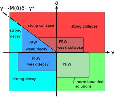
Figure 1: (Color Online) The global asymptotic behavior of solutions in the $\gamma$-$\delta$ plane. The 4th quadrant is characterized by the existence of a limit set in $L^{2}$. Sub-domains sustaining PRW-type waveforms are shown in each quadrant, defined by threshold values $\gamma_{\mathrm{crit}},\delta_{\mathrm{crit}}\sim O(10^{-1})$, at most (cartoon).

Summary on the global dynamics.

According to our analytical arguments given above, we can depict schematically –cf. Fig. 1– the dynamical scenarios for the problem (1)-(3) for the different regimes of the gain/loss parameters.

The limit set is the trivial one, i.e., $\omega(\mathcal{B})=\left\{0\right\}$, in the 2nd quadrant, for $\gamma<\gamma^{*}$ and $\delta>0$, as well as in the 3rd quadrant, for $\gamma,\,\delta<0$. We also note that any solution of Eq. (1) in the form of a continuous wave (cw) is always unstable: indeed, as discussed in Ref. P6 , cw waves either decay or grow in the 1st, 2nd and 3d quadrants of Fig. 1, while for cw amplitude $A=-\gamma/\delta$ in the 4th quadrant, it is prone to the modulational instability (MI). Therefore, such cw solutions could not occur generically, as limit-points $\omega(u_{0})$, included in the attracting set $\omega(\mathcal{B})$. Nevertheless, a broad class of initial conditions of the form:

$$u_{0}(x)=A(x)\exp\left(-\mathrm{i}\frac{K\pi x}{L}\right),\quad K>0,$$ (14)

of amplitude $A(x)$ such that $A(x)\rightarrow h_{0}\neq 0$ as $x\rightarrow\pm\infty$, and wavenumber $K\geq 0$ may lead to plane wave evolution and the manifestation of the corresponding MI effects P6 . We finally note that if $A(x)=$const., then the upper bounds of the collapse times are sharp Achilleos et al. (2015).

III Numerical Results

III.1 Background.

Selecting parameters $\gamma$ and $\delta$ within the dynamical regimes prescribed in Sec. II, we will proceed by numerically studying the dynamics corresponding to algebraically decaying initial data. This is the principal focal point of the present contribution, motivated by our aim to assess the relevance of PRW-type states in models involving driving or gain and damping. More precisely, we will examine the evolution of initial conditions of the following form:

$$u_{0}(x)=h_{0}+\frac{c_{1}}{c_{2}+c_{3}x^{2}},\quad c_{i}>0,\quad i=1,2,3.$$ (15)

The initial condition (15) can be partitioned in two cases: (a) $h_{0}=0$ and (b) $h_{0}>0$, corresponding to a quadratic decay to a vanishing or to a finite background, respectively. The second of the above initial conditions is, in fact, a PRW profile at $t=0$:

$$u_{0}(x)=u_{\mbox{\tiny PS}}(x,t;t_{0};P_{0})|_{t=0}:=\sqrt{P_{0}}\left\{1-\frac{4\left[1+2\mathrm{i}P_{0}(t-t_{0})\right]}{1+4P_{0}x^{2}+4P_{0}^{2}(t-t_{0})^{2}}\right\}\mathrm{e}^{\mathrm{i}P_{0}(t-t_{0})}|_{t=0},$$ (16)

is the PRW solution (translated at $t=t_{0}$) of the integrable NLS, corresponding to $\gamma=\delta=0$.

The PRW is the prototypical solitary waveform, possessing power-law (quadratic) rather than the more standard exponential spatiotemporal localization. For this reason, our aim is to use the PRW profile (16), and employ fitting arguments in the spirit of Ref. P2 , to examine the spatiotemporal growth or decay rate of the numerical solutions of (1)-(3). In this way, our scope is to quantify, starting in the present stage with numerical investigations, the potential robustness of PRW in the presence of perturbations, i.e., for $\gamma,\leavevmode\nobreak\ \delta\neq 0$.

It should also be mentioned that the initial conditions (15) and (16) can be considered as elements of weighted $L^{2}$, or Sobolev spaces, defined as follows. Consider the weight function $w(x)=1+|x|$. Then, the initial conditions (15) or (16) are such that:

$$u_{0}\in X_{w}=\left\{u:\mathcal{Q}\rightarrow\mathbb{C}\;\;:\;\;\int_{\mathcal{Q}}w^{2}(x)|u-h_{0}|^{2}dx<\infty\right\}.$$ (17)

In particular, $u_{0}\in X^{1}_{w}(\mathcal{Q})\cap H^{2}(\mathcal{Q})$, where the weighted Sobolev spaces $X^{m}_{w}$ are defined as:

$$X^{m}_{w}=\left\{u:\mathcal{Q}\rightarrow\mathbb{C}\mbox{:}\;u\in X_{w}\;\;\mbox{and}\;\;\sum_{j=0}^{m}\int_{\mathcal{Q}}w^{2}(x)|\partial^{j}_{x}u|^{2}dx<\infty\right\}.$$

When $L$ is finite but sufficiently large, or $L\rightarrow\infty$, an initial condition $u_{0}\in X^{1}_{w}(\mathcal{Q})\cap H^{2}(\mathcal{Q})$ and its derivative converge with, at least, a quadratic decay-rate to $h_{0}$ and zero, respectively, and has essentially a localization width $\ll 2L$. Note also that, as a consequence of Theorem II.1, the continuous dependence on the initial data in the above space can be stated as:

$$||\mathcal{S}(t)u_{0}-\mathcal{S}(t)u_{1}||_{X^{1}_{w}\cap H^{2}}\leq K(L,T_{0})||u_{0}-u_{1}||_{X^{1}_{w}\cap H^{2}},\quad K(L,T_{0})>0,\quad T_{0}\in[0,T_{\mathrm{max}}),$$ (18)

which will be useful for the analysis of the numerical results: actually we will consider the space $X^{1}_{w}(\mathcal{Q})\cap H^{2}(\mathcal{Q})$ as a potential domain of attraction for PRW-reminiscent waveforms.

Since numerical simulations consider periodic boundary conditions, we should point out that they are satisfied by the initial conditions (15) and (16) (or generically, by elements of $X_{w}$), only asymptotically as $L\rightarrow\infty$. However, the largest error in these asymptotics is of order O$(L^{-2})$. Since the smallest value of $L$ used in our numerical experiments is $L=50$, the error is of order O$(10^{-4})$ or less, and we have confirmed that it has negligible effects in the dynamics.

The numerical experiments have been performed by using a high accuracy pseudo-spectral method, incorporating an embedded error estimator that makes it possible to efficiently determine appropriate step sizes. Regarding the simulations on collapse, we denote as collapse time the time where the numerical scheme detects a singularity in the dynamics. The numerical singularity is detected when the time step is becoming of order $<10^{-12}$.

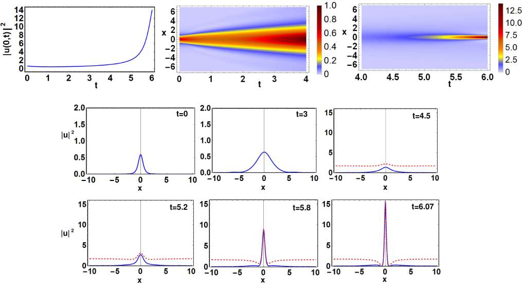
Figure 2: (Color Online) Top row: The left panel shows the evolution of the density of the center, $|u(0,t)|^{2}$, for the initial condition (15), with vanishing background $h_{0}=0$, and $c_{1}=1$, $c_{2}=1.3$, $c_{3}=2$. Parameters $\gamma=0.2$, $\delta=0.01$, $L=50$. The middle and right panels show contour plots for the evolution of the density $|u(x,t)|^{2}$, for the same evolution, as in the left panel. Middle (right) panel corresponds to $t\in[0,4]$ ($t\in[4,6]$). Bottom rows: snapshots of the density $|u(x,t)|^{2}$ [solid (blue) curves] at different times, for the above evolution. The evolution of $|u(x,t)|^{2}$ is compared to that of the PRW $u_{\mbox{\tiny PS}}(x,t;6.07;1.73)$ [dashed (red) curve]. It can be seen that, modulo its absence of background, the central portion of the solitary wave closely resembles, in the vicinity of its peak amplitude time, the PRW structure.

III.2 Collapse regime.

We start our presentation with the case $\gamma,\,\delta>0$ (1st-quadrant in the $\gamma\delta$-plane of Fig. 1), corresponding to the full collapse regime.

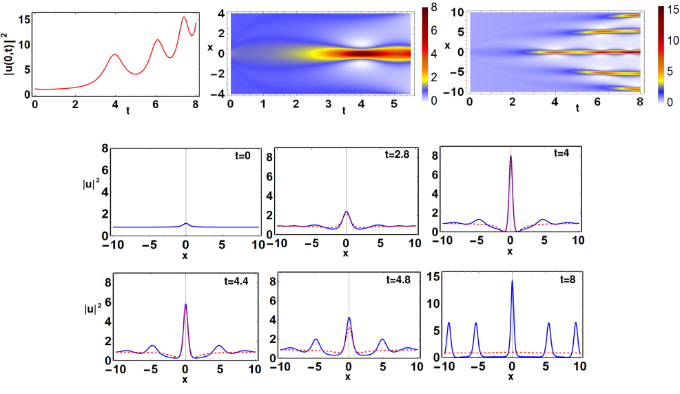
Figure 3: (Color Online) Top row: The left panel shows the evolution of the density of the center, $|u(0,t)|^{2}$, for the initial condition (15), with non-vanishing background $h_{0}=0.9$, and $c_{1}=0.18$, $c_{2}=1$, $c_{3}=3.6$. Parameters $\gamma=0.01$, $\delta=0.01$, $L=50$. The middle and right panels show contour plots for the evolution of the density $|u(x,t)|^{2}$, for the same evolution, as in the left panel. Left (right) panel corresponds to $t\in[0,6]$ ($t\in[0,8]$). Bottom rows: snapshots of the density $|u(x,t)|^{2}$ [solid (blue) curve] at different times, for the above evolution. The evolution of $|u(x,t)|^{2}$ is compared to that of the PRW $u_{\mbox{\tiny PS}}(x,t;4;0.9)$ [dashed (red) curve].

The left panel of the top row of Fig. 2, shows the evolution of the density at the center, $|u(0,t)|^{2}$, for the initial condition (15) with zero-background $h_{0}=0$, and $c_{1}=1$, $c_{2}=1.3$, $c_{3}=2$. The rest of parameters are $\gamma=0.2$, $\delta=0.01$, and $L=50$. Apart from a slight decrease of $|u(0,t)|^{2}$ during the early stages of the dynamics, i.e., within the interval $[0,2]$, we observe an almost monotonic increase, which is typical of a strong collapse Babis : since $|u(0,t)|^{2}$ increases almost monotonically, and the functional $M(t)$ is monotonically increasing as discussed before, most of the initial energy will be concentrated to a single localized structure near the singularity.

Such behavior is illustrated in the middle and the left panel of the top row of Fig. 2, showing contour plots depicting the evolution of the density $|u(x,t)|^{2}$; the middle (right) panel shows the evolution for $t\in[0,4]$ ($t\in[4,6]$), illustrating the initial slight decrease (mentioned above) and the subsequent increase of the amplitude for $t>2$. This behavior is also observed in the snapshots of the evolution of the density [solid (blue) curve], portrayed in the second row. The right panel of this row reveals that as the singularity is approached, the mass becomes progressively concentrated around the center. In addition, we compare the profiles of the numerical solution of (1)-(3) with the PRW profile of the integrable limit, $u_{\mbox{\tiny PS}}(x,t;6.07;1.73)$ [dashed (red) curve]. The value of $P_{0}$ (and $t_{0}$) is selected by simply matching the time (and value) of the maximal density amplitude. This comparison reveals that the time-growth rate, of the numerical solution towards the singularity, is reminiscent of the time-growth rate of the PRW-profile. It is also interesting to observe that the localized structure forms, towards collapse, a PRW-core (with a suitably adapted spatial distribution), as shown in the last snapshot at $t=6.07$. This phenomenon will be further discussed below.

The structure of collapse appears to be totally different in the case of a finite background $h_{0}>0$. The left panel of the top row of Fig. 3 reveals that, in contrast to the case $h_{0}=0$, the evolution of the density at the center, $|u(0,t)|^{2}$, is not monotonic. The initial condition corresponds to $h_{0}=0.9$, with $c_{1}=0.18$, $c_{2}=1$, $c_{3}=3.6$, while the rest of parameters are $\gamma=0.01$, $\delta=0.01$ and $L=50$. The evolution in this case suggests a drastically different event prior to collapse, which we can describe as follows. Here, $|u(0,t)|^{2}$ exhibits a local maximum at $t\simeq 4$ and a local minimum at $t\simeq 5$, yet the functional $M(t)$ is strictly increasing. Hence, the decrease of the center density is followed by a partial transfer to emergent localized side lobes adjacent to the center, while $M(t)$ remains increasing. Therefore, the type of collapse should be weak, with the formation of tails consisting of localized waveforms.

The dynamics in this case is shown in the rest of the panels of Fig. 3. There, the differences between the present and the previous case are highlighted: in the present case, a weak-type of collapse is observed, as explained above and shown in the snapshot at $t=8$. Furthermore, another remarkable feature is that, even in this case, a PRW-type wave form appears to emerge. The comparison between the numerical solution of Eq. (1) and the PRW $u_{\mbox{\tiny PS}}(x,t;4;0.9)$ within the time interval $[2.8,4.8]$ reveals that the centered localized structure possesses a spatiotemporal growth/decay rate, reminiscent of that of the PRW. This can be attributed to the continuous dependence on the initial data $u_{0}$. At the same time, this intriguing observation seems to indicate that the PRW structure is a transient precursor arising “en route” to collapse dynamics. This is related to the broader scale question about to which extent, extreme (yet finite amplitude) events, such as the PRW, may catalyze –if present– the transition towards collapse. As seen in Fig. 3 and discussed above, the continuous dependence on initial data (18), along with the monotonic growth of $M(t)$, lead to a central peak that tends to gain energy from the finite background. At the same time, the dynamics of the –generic, here– modulational instability, recently analyzed in its nonlinear stage in the work of Ref. BM , suggests the division of the spatial domain into three regions. These are a far left field and a far right field, in which the solution is approximately equal to its initial value, as well as a central region in which the solution has oscillatory behavior with respect to the spatial variable $x$. While the situation here is complicated due to the presence of the gain and loss, a similar division of the domain is portrayed –cf. top right contour plot of Fig. 3. Nevertheless, we observe time-oscillations of increasing amplitude. In summary, the competition between the effects of core gain and side-band growth due to MI, results in a non-monotonic scenario for the increase of the core amplitude; this increase, combined with the manifestation of MI, is also accompanied by the emergence of side humps, of also increasing oscillatory amplitude. However, the growth rate of the eventually collapsing core, is larger than the growth rate of the developing humps.

It is important to remark, that the above type of weak collapse, and the emergence of a PRW-type wave form, persists up to small values of $\gamma>\gamma^{*}$ and $\delta>0$, i.e., up to critical thresholds $\gamma_{\mathrm{crit}},\delta_{\mathrm{crit}}\sim O(10^{-2})$. Beyond that critical values, the growth of $|u(0,t)|^{2}$ becomes again monotonic, reminiscent to that discussed in the example of Fig. 2, and a strong type of collapse is again manifested. This is a first evidence that PRW-type dynamics may emerge in $\gamma,\delta$-parametric regimes, close to the NLS integrable limit.

Concerning the behavior of the analytical upper bounds (8)-(10) of the collapse times, when implemented for localized initial data, we remark that the type of collapse for such data [with either algebraic as (15), or exponential decay as in Achilleos et al. (2015)], does not follow the ODE dynamics of the homogeneous background. This effect is generically reflected in discrepancies between the numerical blow-up times and the upper bounds, and analyzed in (Achilleos et al., 2015, Sec.3.2, pg. 62).

III.3 Decay regime.

We now turn to the decay regime, once again distinguishing between initial data with $h_{0}=0$ and $h_{0}\neq 0$. When $h_{0}=0$, we observe decay, as shown in the left panel of Fig. 4. This figure depicts the monotonic decay of the center density, $|u(0,t)|^{2}$, and insets show characteristic density snapshots at specific times. The rest of the parameters for the initial condition are $c_{1}=1$, $c_{2}=1.3$, $c_{3}=2$, as in the case of collapse in finite time of Fig. 2, for $\delta=0.01$ and $\gamma>\gamma^{*}\simeq 0$. However, while still $\delta=0.01$ as in the collapse example, the parameter $\gamma=-0.01<\gamma^{*}$ leads to decay dynamics. Clearly, this example highlights the accuracy of the analytically defined “separatrix”, distinguishing collapse from decay in the 2nd quadrant in the $\gamma\delta$-plane of Fig. 1. The decay is now explained by reversing the argument used for the strong collapse of Fig. 2: since $|u(0,t)|^{2}$ is monotonically decreasing, the profiles should flatten prior to decay, so as to follow the monotonic decrease of the averaged power functional $P_{a}[u(t)]$ [cf. Eq. (13)].

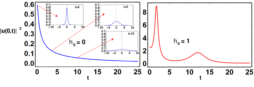
Figure 4: (Color Online) Left panel: monotonic decay for the initial condition (15) with vanishing background $h_{0}=0$, and $c_{1}=1$, $c_{2}=1.3$, $c_{3}=2$; other parameters: $\gamma=-0.01<\gamma^{*}\simeq 0$, $\delta=0.01$. The solid (blue) curve depicts the evolution of the center density $|u(0,t)|^{2}$. Arrows are directed to insets portraying snapshots of the density $|u(x,t)|^{2}$ at $t=0$ (initial condition), $t=3$ and $t=10$. Right panel: non-monotonic decay for an initial condition (15) with finite background $h_{0}=1$ and $c_{1}=0.8$, $c_{2}=1.3$ and $c_{3}=2$; rest of parameters $\gamma=-0.03$, $\delta=-0.01$ (full decay regime), and $L=50$. Emergence of an extreme event occurs at $t=1.625$.

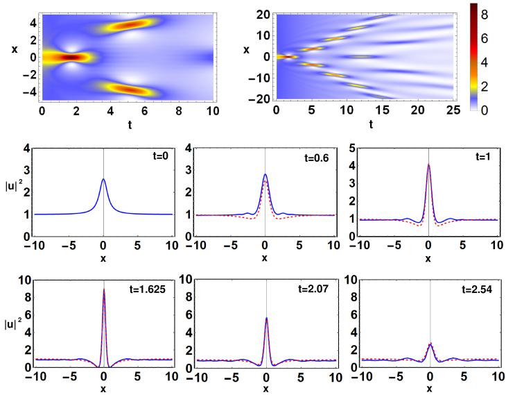
Figure 5: (Color Online) Top row: contour plots for the evolution of the density $|u(x,t)|^{2}$, for the initial condition (15), with non-vanishing background $h_{0}=1$, and $c_{1}=0.8$, $c_{2}=1.3$, $c_{3}=2$; other parameters: $\gamma=-0.03$, $\delta=-0.01$, $L=50$. Left (right) panel corresponds to $t\in[0,10]$ ($t\in[0,25]$). Bottom rows: numerically obtained density snapshots [solid (blue) curves] are compared to those of the PRW, $u_{\mbox{\tiny PS}}(x,t;1.625;1)$ [dashed (red) curves].

Rather surprisingly, when the initial condition features a finite background $h_{0}>0$, the emergence of a PRW-type waveform is observed in the full decay regime $\gamma<0,\,\delta<0$ (3rd quadrant in Fig. 1). This is particularly interesting from a physical point of view: in this regime, Eq. (1) describes a realistic situation, namely the evolution of pulses or beams in nonlinear optical media featuring linear loss and two-photon absorption, which are generic dissipative effects in the context of optics Agrawal (2003); Kivshar & Agrawal (2003).

The right panel of Fig. 4 depicts the non-monotonic decay of the center density $|u(0,t)|^{2}$ for an initial condition (15), with $h_{0}=1$, $c_{1}=0.8$, $c_{2}=1.3$ and $c_{3}=2$; the loss parameters are $\gamma=-0.03$ and $\delta=-0.01$. Evidently, an extreme event occurs at $t=1.625$ and precedes the eventual decay dynamics of this example. This is analyzed further in Fig. 5. The first row shows contour plots for the evolution of the density. In particular, the left panel shows the evolution at early times, i.e., for $t\in[0,10]$, illustrating the emergence of an extreme event (cf. peak of the center density in the right panel of Fig. 4); the right panel illustrates the evolution of the density for $t\in[0,25]$, depicting the structure of the decaying dynamics. In the bottom rows, snapshots of $|u(x,t)|^{2}$ for $t\in[0,2.54]$ are portrayed, and are compared to the evolution of the PRW, $u_{\mbox{\tiny PS}}(x,t;1.625;1)$. The comparison clearly supports the identification of the emerging structure around the peak formation as one of the Peregrine family. The centered localized waveform of the numerical solution, preserves the algebraic spatial decay of the initial condition, but also exhibits an algebraic in time growth/decay rate: notably, both the time-growing, and then time-decaying, centered profiles appear to manifest a locking to a PRW-type mode, whose maximum density is attained at $t=1.625$. For $t\in(1.625,2.54]$, the algebraic-in-time decay rate remains close to that of the PRW.

It is relevant to mention here, that the excitation of a PRW-type event, by localized initial data on the top of a finite background, was observed in Yang1 , for a non-integrable, higher-order NLS equation. The initial condition in Yang1 is an interaction between a Gaussian-type pulse of small amplitude and a cw. It was shown that when the width of the initial perturbation pulse is wide enough, a PRW can be excited. In the same spirit, the evolution of a rational fraction pulse, extracted from the analytical PRW-solution, was investigated in Yang2 .

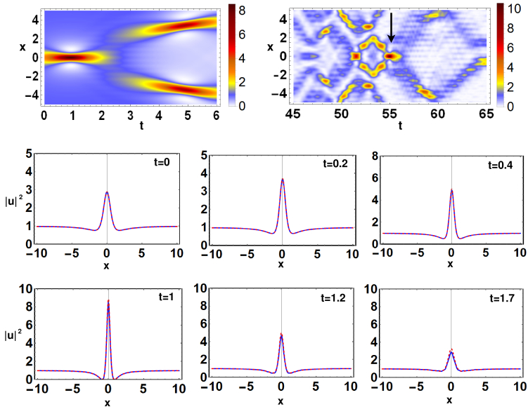
Figure 6: (Color Online) Top row: contour plots for the evolution of the density, $|u(x,t)|^{2}$, for the initial condition (16), $u_{0}(x)=u_{\mbox{\tiny PS}}(x,0;-0.9;1)$; other parameters: $\gamma=0.01$, $\delta=-0.01$ (limit set regime), and $L=50$. Left (right) panel corresponds to $t\in[0,6]$ ($t\in[45,65]$). Bottom rows: numerically obtained density snapshots [solid (blue) curves] are compared to those of the PRW, $u_{\mbox{\tiny PS}}(x,t;-0.9;1)$ [dashed (red) curves].

In light of the results of Yang1 , here, we see the combination of the following effects: the proximity of the initial condition to the PRW, and of the model to the integrable NLS, which apparently drive the growth of the Peregrine phase, and –at the same time– the role of the $\gamma$ and $\delta$ terms in enforcing the monotonic decay of the functional $P_{a}[u(t)]$. As a result, the transient initial growth eventually gives way to the expected long-time decay of the model data. The considerations of BM regarding the manifestation of MI are still applicable in this full decay regime, explaining the right contour plot of Fig. 5. However, the dynamics is eventually overwhelmed by loss events, hence the effect of MI is suppressed.

As in the case of the collapse regime, it should also be remarked that the emergence of extreme events reminiscent of PRW, persists up to a critical threshold of $\gamma_{\mathrm{crit}},\delta_{\mathrm{crit}}\sim O(10^{-1})$ (i.e., for a higher order of magnitude of $|\gamma|,\;|\delta|$, than in the collapse regime). However, the amplitude of the PRW-type event is decreasing, as we approach these critical values. Furthermore, beyond these critical values, the solution preserves its structural form during decay. We qualitatively consider such thresholds as distinguishing between the near-integrable NLS-based regime, where gain and loss bear a more perturbative role (even if asymptotically dominating) to the NLS dynamics –at least in short/intermediate time scales– and a fundamentally different regime. In the latter, the gain/loss parameters play a more drastic role, and may completely suppress the integrable features, including the potential formation of Peregrine-type structures.

III.4 Limit Set Regime.

Let us finally consider the global existence regime $\gamma>0$, $\delta<0$, which is generically associated with the nontrivial limit set $\omega(\mathcal{B})$, discussed in Sec. II. In this regime, we choose parameter values $\gamma=0.01$, $\delta=-0.01$, and examine the evolution of an initial condition (16), namely $u_{0}(x)=u_{\mbox{\tiny PS}}(x,0;-0.9;1)$. The snapshots of the evolution of the density in Fig. 6 show that the numerical solution of the nonintegrable Eq. (1) fits very well the PRW of the integrable limit, for $t\in[0,1.7]$.

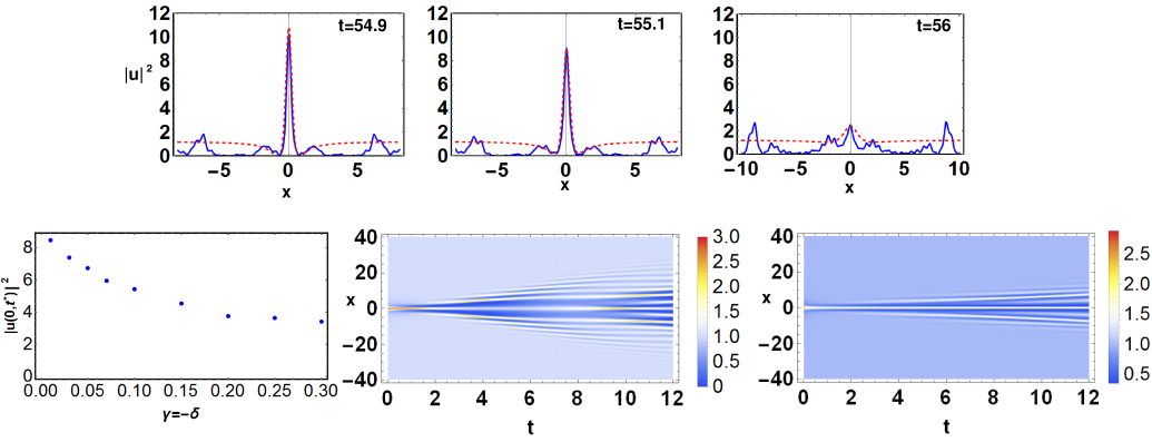
Figure 7: (Color Online) Top row: Density snapshots corresponding to the evolution of the Fig. 6, for $t\in[54.6,56]$. Density $|u(x,t)|^{2}$ [solid (blue) curve] is compared to the evolution of the PRW, $u_{\mbox{\tiny PS}}(x,t;54.9;1.2)$ [dashed (red) curve]. Bottom row: the left panel depicts the decrease of the maximum of the density $|u(0,t^{*})|^{2}$, of the first localized event, for increasing values of $\gamma=-\delta$. The middle and right panels, show contour plots of the evolution of the density $|u(x,t)|^{2}$, when $\gamma=-\delta=0.4$, and $\gamma=-\delta=1.5$, respectively. In all panels, the initial condition, and the rest of parameters, are fixed as in Fig. 6.

This PRW-type structure corresponds to the first extreme event detected in the left panel of the first row of Fig. 6. Another interesting extreme event emerges at $t\approx 54$, long after the MI has taken over, and led the entire domain to a highly nonlinear, apparently chaotic phenomenology. This event is pointed out by the (black) arrow in the right panel of the first row of Fig. 6. Figure 7 shows density snapshots of this structure for $t\in[54.6,56]$, which are compared to the density evolution of the PRW of the integrable limit, $u_{\mbox{\tiny PS}}(x,t;54.9;1.2)$. Note that the maximum of the numerical solution in this time interval, is attained at $t\approx 54.9$. The centered localized waveform, possesses a growth/decay rate in time, still reminiscent of the PRW. In the vicinity of specific times (such as $t=54.9$ –where the maximum is attained– or $t=55.1$), its profile is quite reminiscent of that of the PRW.

Similarly to the cases of the collapse and decay regimes, there are threshold values $\gamma_{\mathrm{crit}},\delta_{\mathrm{crit}}\sim O(10^{-1})$ (i.e., of the same order of magnitude as in the decay regime), for the persistence of PRW-type dynamics. An illustrative example is portrayed in the bottom row of Figure 7: the first panel shows the decrease of the maximum density $|u(0,t^{*})|^{2}$, of the center of the first localized event (achieved at a specific time $t^{*}$), as $\gamma=-\delta$ increases (i.e., as we consider increasing values along the diagonal on the 4th quadrant $\gamma>0$, $\delta<0$). The initial condition, and the rest of parameters, are fixed as in Fig. 6. For increased values of $\gamma=-\delta$, the amplitude of the centered localized structure oscillates, but within moderate values, as depicted in the contour plot of the middle panel, corresponding to the case $\gamma=-\delta=0.4$. For even larger values, the amplitude is tending to a stabilization, and the dynamics are closely reminiscent to that of (BM, , Fig. 3, pg. 043902-4), for the integrable NLS-limit. Such dynamics are portrayed in the contour plot of the right panel, corresponding to the case $\gamma=-\delta=1.5$.

Movies, related to the numerical findings illustrated in this Section, can be found in M4a -M9 .

IV Discussion and Conclusions

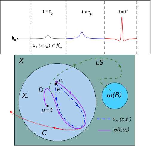
Figure 8: (Color Online) Top panel: An initial condition $u_{0}(x,t_{0})\in X_{w}$, evolves towards a waveform reminiscent of the PRW, achieving its maximum at $t=t^{*}$ (cartoon). Bottom panel: A potential PRW-type solution $u_{\mbox{\tiny PS}}(x,t)$ of (1), viewed as an unstable “homoclinic loop” [dashed (blue) curve]], connecting $P_{0}$ (cartoon).

In the present work, we have considered the dynamics of a nonlinear Schrödinger (NLS) model, incorporating linear and nonlinear gain/loss, and supplemented with periodic boundary conditions. The model finds applications in nonlinear optics, where it describes evolution of pulses or beams in optical media with gain and loss (e.g., linear gain or loss, two-photon absorption, etc).

We started our exposition by outlining the parametric regimes for the existence of a nontrivial (attracting) limit set, decay, and finite time collapse. Then, we examined numerically, in all the above regimes, the dynamics stemming from initial data with algebraic localization. The two broad classes of initial data considered were those decaying to zero and those converging to a finite background. Collapse and decay were explored in both regimes and significant differences between them were found. In particular, for the former case of initial conditions the solution preserves its structural form during decay, or develops almost strong collapse. For the latter case of initial data, the solution decays without preserving its form, or is subject to a weak-type of collapse. The emerging profiles at the early stage of the evolution were analyzed by considering the combination of the monotonicity properties of suitably defined functionals and the modulational instability of the background. It was thus found that oscillatory central density dynamics can occur, as shown in our detailed numerical simulations.

Furthermore, in a broad array of gain/loss parametric regimes, we have identified the emergence of transient, spatiotemporally localized waveforms reminiscent of the Peregrine rogue wave (PRW) of the integrable NLS limit. Indeed, in a diverse array of scenarios, we have exhibited temporal, as well as spatial growth and decay rates that are highly proximal to PRWs for finite time intervals. This strongly suggests that the Peregrine structures remain highly relevant for the dynamics beyond their “exact” realm of the integrable limit, as it was first reported in Yang1 , for the case of non-integrable higher-order NLS. That being said, upon sufficient departure from that parametric range, the gain/loss appear to overwhelm the dynamics and destroy the potential of manifestation of PRW-type structures.

This main finding, can be schematically depicted in two ways. The first, is illustrated in the top panel of Fig. 8: an initial condition $u_{0}(x,t_{0})\in X_{w}$, may evolve towards a waveform reminiscent of the PRW, achieving its maximum at $t=t^{*}$. The weighted subspace $X_{w}$ of the infinite dimensional phase space $X$ for the extended dynamical system associated to Eq. (1), describes the algebraic spatial localization of the initial condition. The second, can be portrayed in the “phase diagram” of the system shown in the bottom panel of Fig. 8. A potentially existing PRW-type solution [dashed-dotted (blue) curve], is marked by $u_{\mbox{\tiny PS}}(x,t)$. It can be visualized as a “homoclinic loop” connecting the unstable background of density $P_{0}$. The solution $u_{\mbox{\tiny PS}}(x,t)$ is an element in the weighted subspace $X_{w}$, which is a potential domain of attraction for such solutions. An initial condition $u_{0}\in X_{w}$, can be selected to start nearby the orbit $u_{\mbox{\tiny PS}}(x,t)$. This, follows a path $\phi(t,u_{0})$ [continuous (magenta) curve], which remains close to the orbit $u_{\mbox{\tiny PS}}(x,t)$, for a finite-time interval.

In this picture, the ultimate fate of the path $\phi(t,u_{0})$, depends on the selected parametric regime for $\gamma$, $\delta$. In the decay regime, the path $\phi(t,u_{0})$ stays close to the orbit $u_{\mbox{\tiny PS}}(x,t)$ for a finite time interval, but then diverges through the branch $D$ [continuous (magenta) curve], to the trivial state $u=0$. In the collapse regime, the path $\phi(t,u_{0})$ stays close to the orbit $u_{\mbox{\tiny PS}}(x,t)$ for shorter times, and then diverges towards collapse, through the branch $C$ [dotted (red) curve]. Finally, in the limit set regime, the path $\phi(t,u_{0})$ stays close to the orbit $u_{\mbox{\tiny PS}}(x,t)$ for a finite interval, and then, it converges to the nontrivial attracting set $\omega(\mathcal{B})$, through the branch $LS$ [dashed (green) curve].

The present study, opens a number of questions for future investigations. An important one, concerns the development of analytical approximations to determine such PRW-type solutions, or the derivation of analytical estimates on the spatiotemporal growth/decay rates observed numerically. This is part of the broader question regarding the persistence of rational solutions in models beyond the integrable limit, such as the one of the NLS and, e.g., of the massive Thirring model alejandro .

Another interesting and relevant direction, is to explore the possibility of generalizing this approach to other models, such as extended NLS equations incorporating higher-order effects devine ; P6 ; Yang1 ; Yang2 ; themis , or even to discrete setups P4 ; P7 . Appreciating the robustness of rogue waves under both perturbations in initial data and perturbations in the models/parameters is thus currently a broader theme under consideration, and relevant conclusions will be reported in future work.

Acknowledgments. We would like to thank the referees for valuable comments. The authors Z.A.A., G.F., D.J.F., N.I.K., P.G.K., I.G.S. and K.V., acknowledge that this work made possible by NPRP grant # [8-764-160] from Qatar National Research Fund (a member of Qatar Foundation). The findings achieved herein are solely the responsibility of the authors. D.J.F. and P.G.K. gratefully acknowledge the support of the “Greek Diaspora Fellowship Program” of Stavros Niarchos Foundation.

References

- Hasegawa & Kodama (1996) A. Hasegawa and Y. Kodama, Solitons in optical communications (Oxford University Press, 1996).
- Agrawal (2003) G. P. Agrawal, Nonlinear Fiber Optics (Academic Press, 2012).
- Kivshar & Agrawal (2003) Yu. S. Kivshar and G. P. Agrawal, Optical Solitons: From Fibers to Photonic Crystals (Academic Press, 2003).
- (4) N. N. Akhmediev and A. Ankiewicz, Solitons. Nonlinear Pulses and Beams (Chapman and Hall, 1997).
- (5) L. Gagnon, J. Opt. Soc. Am. B 10, 469 (1993).
- (6) D. H. Peregrine, J. Austral. Math. Soc. B 25, 16 (1983).
- (7) E. A. Kuznetsov, Sov. Phys.-Dokl. 22, 507 (1977).
- (8) Y. C. Ma, Stud. Appl. Math. 60, 43 (1979).
- (9) N. N. Akhmediev, V. M. Eleonskii, and N. E. Kulagin, Theor. Math. Phys. 72, 809 (1987).
- (10) K. B. Dysthe and K. Trulsen, Phys. Scr. T82, 48 (1999).
- (11) E. Pelinovsky and C. Kharif (eds.), Extreme Ocean Waves (Springer, New York, 2008).
- (12) C. Kharif, E. Pelinovsky, and A. Slunyaev, Rogue Waves in the Ocean (Springer, New York, 2009).
- (13) A. R. Osborne, Nonlinear Ocean Waves and the Inverse Scattering Transform (Academic Press, Amsterdam, 2010).
- (14) M. Onorato, S. Residori, F. Baronio, Rogue and Shock Waves in Nonlinear Dispersive Media (Springer-Verlag, Heidelberg, 2016).
- (15) A. Chabchoub, N. P. Hoffmann, and N. Akhmediev, Phys. Rev. Lett. 106, 204502 (2011).
- (16) A. Chabchoub, N. Hoffmann, M. Onorato, and N. Akhmediev, Phys. Rev. X 2, 011015 (2012).
- (17) A. Chabchoub and M. Fink, Phys. Rev. Lett. 112, 124101 (2014).
- (18) D. R. Solli, C. Ropers, P. Koonath, and B. Jalali, Nature 450, 1054 (2007).
- (19) B. Kibler et al., Nature Phys. 6, 790 (2010).
- (20) B. Kibler et al., Sci. Rep. 2, 463 (2012).
- (21) J. M. Dudley, F. Dias, M. Erkintalo, and G. Genty, Nat. Photon. 8, 755 (2014).
- (22) B. Frisquet et al., Sci. Rep. 6, 20785 (2016).
- (23) C. Lecaplain, Ph. Grelu, J. M. Soto-Crespo, and N. Akhmediev, Phys. Rev. Lett. 108, 233901 (2012).
- (24) A. N. Ganshin, V. B. Efimov, G. V. Kolmakov, L. P. Mezhov-Deglin, and P. V. E. McClintock, Phys. Rev. Lett. 101, 065303 (2008).
- (25) H. Bailung, S. K. Sharma, and Y. Nakamura, Phys. Rev. Lett. 107, 255005 (2011).
- (26) A. Ankiewicz, N. Devine, N. Akhmediev, Phys. Lett. A 373, 3997 (2009).
- (27) A. Ankiewicz, Y. Wang, S. Wabnitz, and N. Akhmediev, Phys. Rev. E 89, 012907 (2014).
- (28) L. H. Wang, K. Porsezian, and J. S. He, Phys. Rev. E 87, 053202 (2013).
- (29) Y. Yang, Z. Yan and B. A. Malomed, Chaos 25, 103112 (2015).
- (30) Y. Wang, L. Song, L. LI and B. A. Malomed, J. Opt. Soc. Am. B 32, 2257 (2015).
- (31) A. Calini and C. M. Schober, pp. 31–51 in Ref. k2a .
- (32) J. Garnier and K. Kalimeris, J. Phys. A: Math. Theor. 45, 035202 (2012).
- (33) J. Cuevas-Maraver, P.G. Kevrekidis, D.J. Frantzeskakis, N.I. Karachalios, M. Haragus, G. James, https://arxiv.org/abs/1701.06212.
- (34) M. Onorato and D. Proment, Phys. Lett. A 376, 3057 (2012).
- (35) E. Zakharov and L. A. Ostrovsky, Phys. D 238, 540 (2009).
- (36) M. Brunetti, N. Marchiando, N. Berti, J. Kasparian, Phys. Lett. A 378, 1025 (2014).
- (37) A. Slunyaev, A. Sergeeva and E. Pelinovsky, Phys. D 303, 18 (2015).
- (38) A. Calini and C. M. Schober, Nonlinearity 25, R99 (2012).
- (39) A. Islas and C.M. Schober, Phys. D 240, 1041 (2011).
- (40) C. Eigen, A. L. Gaunt, A. Suleymanzade, N. Navon, Z. Hadzibabic, and R. P. Smith, Phys. Rev. X 6, 041058 (2016).
- (41) G. Yang, L. Li and S. Jia, Phys. Rev. E 85, 046608 (2012).
- (42) G. Yang, Y. Wang, Z. Qin, B. A. Malomed, D. Mihalache and L. Li, Phys. Rev. E 90, 062909 (2014).
- (43) R. Hirota, J. Math. Phys. 14, 805 (1973).
- (44) E. G. Charalampidis, J. Cuevas-Maraver, D. J. Frantzeskakis and P. G. Kevrekidis, https://arxiv.org/abs/1609.01798.
- Cazenave (2003) T. Cazenave, Semilinear Schrödinger equations, Courant Lecture Notes 10 (Amer. Math. Soc., 2003).
- Kato (1975) T. Kato, Quasilinear equations of evolution with applications to partial differential equations, Lecture Notes in Mathematics 448, pp. 25–70 (Springer-Verlag, New York, 1975).
- (47) V. Achilleos, A. R. Bishop, S. Diamantidis, D. J. Frantzeskakis, T. P. Horikis, N. I. Karachalios, and P. G. Kevrekidis Phys. Rev. E 94, 012210 (2016).
- Achilleos et al. (2015) V. Achilleos, S. Diamantidis, D. J. Frantzeskakis, T. P. Horikis, N. I. Karachalios, and P. G. Kevrekidis, Phys. D 316, 57 (2016).
- (49) G. Biondini and D. Mantzavinos. Phys. Rev. Lett. 116, 043902 (2016).
- (50) Strong collapse, Fig. 2. Initial evolution: http://myria.math.aegean.gr/~karan/Fig4a.gif.
- (51) Strong collapse, Fig. 2. Comparison with PRW: http://myria.math.aegean.gr/~karan/Fig4b.gif.
- (52) Weak collapse, Fig. 3. (a) Emergence of the first event: http://myria.math.aegean.gr/~karan/Fig5a.gif.
- (53) Weak collapse, Fig. 3. Continued from (a): http://myria.math.aegean.gr/~karan/Fig5b.gif.
- (54) Decay regime, Fig. 5. http://myria.math.aegean.gr/~karan/Fig7.gif
- (55) Limit-set regime, Fig. 6. PRW initial condition: http://myria.math.aegean.gr/~karan/Fig8.gif
- (56) Limit-set regime, Fig. 7. MI dynamics: http://myria.math.aegean.gr/~karan/Fig9.gif
- (57) A. Degasperis, A.B. Aceves, and S. Wabnitz, Phys. Lett. A 379, 1067 (2015).
- (58) W. Cousins and T.P. Sapsis, Phys. Rev. E 91, 063204 (2015).
- (59) Yannan Shen, P.G. Kevrekidis, G.P. Veldes, D.J. Frantzeskakis, D. DiMarzio, X. Lan, V. Radisic, https://arxiv.org/abs/1612.00031.
- (60) G. P. Veldes, J. Cuevas, P. G. Kevrekidis, and D. J. Frantzeskakis. Phys. Rev. E 88, 013203 (2013).