Magnon-photon coupling in antiferromagnets

Abstract

Magnon-photon coupling in antiferromagnets has many attractive features that do not exist in ferro- or ferrimagnets. We show quantum-mechanically that, in the absence of an external field, one of the two degenerated spin wave bands couples with photons while the other does not. The photon mode anticrosses with the coupled spin waves when their frequencies are close to each other. Similar to its ferromagnetic counterpart, the magnon-photon coupling strength is proportional to the square root of number of spins $\sqrt{N}$ in antiferromagnets. An external field removes the spin wave degeneracy and both spin wave bands couple to the photons, resulting in two anticrossings between the magnons and photons. Two transmission peaks were observed near the anticrossing frequency. The maximum damping that allows clear discrimination of the two transmission peaks is proportional to $\sqrt{N}$ and it’s well below the damping of antiferromagnetic insulators. Therefore the strong magnon-photon coupling can be realized in antiferromagnets and the coherent information transfer between the photons and magnons is possible.

Information transfer between different information carriers is an important topic in information science and technology. This transfer is possible when strong coupling exists among different information carriers. Strong coupling has already been realized between photons and various excitations of condensed matter including electrons, phonons, Tolpygo1950 ; Kun1951 plasmons Ritchie1957 ; Barnes2003 ; Berini2011 , superconductor qubits Wallraff2004 , excitons in a quantum well Dufferwiel2015 and magnons Soykal2010 ; Huebl2013 ; Cao2015 . Among all of the excitations, magnons, which are excitations of the magnetization of a magnet, are promising information carriers in spintronics because of their low energy consumption, long coherent distance/time, nanometer-scale wavelength, and useful information processing frequency ranging from gigahertz (GHz) to terahertz (THz). Furthermore, magnons can also be a control knob of magnetization dynamics yanpeng2011 ; hubin2013 ; xiansi2012 , and magnon bands of a magnet can be well controlled by either magnetic field or electric current. The electric field $\mathbf{E}$ and magnetic inductance $\mathbf{B}$ in a microcavity of volume $V$ can be sufficient strong even with only one or a few photons of frequency $\nu$ ($|\mathbf{E}|$, $|\mathbf{B}|\propto\sqrt{h\nu/V}$). Therefore, the coupling between the microcavity photons and the magnons of nanomagnets have received particular attention in recent years. Moreover, similar to the cavity quantum electrodynamics Walther2006 which deals with coupling between photons and atoms in a cavity and provides a useful platform for studying quantum phenomenon and for various applications in micro laser and photon bandgap structure, cavity magnonics is also a promising arena for investigating magnons at the quantum level and for manipulating information transfer between single photon and single magnon.

The theoretical demonstration of a possible coupling of a ferro-/ferrimagnet to light was provided in 2013 Soykal2010 . The coupling strength is proportional to the square root of the number of spins $\sqrt{N}$ and the coupling energy could be as big as $\sim 100\ \mu eV$ in a cavity of $\sim 1$ mm and resonance frequency $\sim 200$ GHz. The prediction was experimentally confirmed by placing a yttrium iron garnet (YIG) particle in a microwave cavity of high quality factor. Tabuchi2014 ; Zhang2014 ; Bai2015 ; Huebl2013 Many applications based on these results have been proposed, including the generation and characterization of squeezed states through the interaction between magnons and superconducting qubits via microwave cavity photons Tabuchi2014 and coherent information transfer between magnons and photons Zhang2014 . The information can be transmitted and read out electrically in the hybrid architecture under a strong magnon-photon coupling. Flaig2016

Antiferromagnets (AFM) have many useful properties in comparison with ferromagnetic materials such as better stability against the external field perturbations and negligible cross talking with the neighboring AFM elements because of the absence of stray fields. The AFM dynamics is typically of the order of THz, much faster than the order of GHz for ferromagnets. Because of these superb properties, various aspects of antiferromagnetic spintronics have attracted significant interests in the last few years including domain wall motion, skyrmions, magnetoresistence, magnetic switching, spin pumping, spin current transport and so on. Jungwirth2016 However, only few works based on the classical electrodynamics were reported on the magnon-photon coupling Manohar1972 ; Bose1975 in AFM so far. In order to have a better understanding of the magnon-photon coupling in AFM, we would like to study the issue at the quantum level. In this letter, we demonstrate quantum mechanically the existence of magnon-polariton in an AFM and show that there exists a dark mode and a bright mode in the strong coupling regime. Antiferromagnetic insulators with low damping are promising candidates to realize strong magnon-photon coupling.

We consider a two sublattice antiferromagnet whose spins on the sublattices ($a$ and $b$) align in the opposite directions along $\pm z$-axis as shown in Fig. 1. The Hamiltonian of the AFM coupled with light through its magnetic field is

$$H=H_{\mathrm{AFM}}+H_{\mathrm{ph}}+H_{\mathrm{int}},$$ (1)

$$H_{\mathrm{AFM}}=J\sum_{l,\delta}(\mathbf{S}_{l}^{a}\cdot\mathbf{S}_{l+\delta}^{b}+\mathbf{S}_{l}^{b}\cdot\mathbf{S}_{l+\delta}^{a})$$

$$\ -\sum_{l}(\mathbf{H}_{0}+\mathbf{H}_{a})\cdot\mathbf{S}_{l}^{a}-\sum_{l}(\mathbf{H}_{0}-\mathbf{H}_{a})\cdot\mathbf{S}_{l+\delta}^{b}$$

$$H_{\mathrm{ph}}=\frac{1}{2}\int\left(\epsilon_{0}\mathbf{E}^{2}+\frac{1}{\mu_{0}}\mathbf{B}^{2}\right)\mathrm{d}x\mathrm{d}y\mathrm{d}z$$

$$H_{\mathrm{int}}=-\sum_{l,\alpha=a,b}\mathbf{S}_{l}^{\alpha}\cdot\mathbf{H}_{f}$$

where $H_{\mathrm{AFM}}$, $H_{\mathrm{ph}}$, $H_{\mathrm{int}}$ are respectively the Hamiltonian for AFM, photon and their interaction. $J$ ($>0$) is the exchange constant, $\mathbf{S}_{l}^{a}$ and $\mathbf{S}_{l}^{b}$ are the spins on sites $l$ of sublattices $a$ and $b$ respectively. $\delta$ denotes the displacement of two nearest spins. $\mathbf{H}_{0}$ is the external magnetic field and $\mathbf{H}_{a}$ is the anisotropy field. $\mathbf{E}$ and $\mathbf{B}$ are the electric field and magnetic inductance of the electromagnetic (EM) wave and $\mathbf{H}_{f}$ is the corresponding magnetic field, $\epsilon_{0}$ and $\mu_{0}$ are vacuum permittivity and susceptibility, respectively.

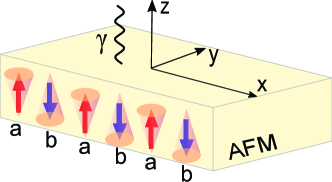
Figure 1: (color online) Sketch of an antiferromagnetic Néel state interacted with light. The $x,y,z$ axes are respectively along the length, width, and thickness directions of the AFM strip. The red and blue arrows, respectively pointing to the $+z$ and $-z$ orientations, represent spins on sublattices $a$ and $b$.

Using the Holstein-Primakoff transformation Holstein1940 , $H_{\mathrm{AFM}}$ in the momentum space can be written as

$$H_{\mathrm{AFM}} =H_{\mathrm{ex}}\sum_{q}\left[\gamma_{q}(a_{q}^{\dagger}b_{q}^{\dagger}+a_{q}b_{q})+(a_{q}^{\dagger}a_{q}+b_{q}^{\dagger}b_{q})\right]$$ (2)

$$+\sum_{q}\left[(H_{a}+H_{0})a_{q}^{\dagger}a_{q}+(H_{a}-H_{0})b_{q}^{\dagger}b_{q}\right],$$

where $H_{\mathrm{ex}}=2JSz$, $z$ and $\gamma_{q}$ are respectively the coordination number and the structure factor of the lattice. The EM wave could be quantized through the standard procedures $H_{\mathrm{ph}}=\hbar\sum_{q}\omega_{q}\left(c_{q}^{\dagger}c_{q}+\frac{1}{2}\right)$ and the interaction term is $H_{\mathrm{int}}=\hbar\sum_{q}g_{c}\left(c_{q}a_{q}+c_{q}^{\dagger}a_{q}^{\dagger}+c_{q}b_{q}^{\dagger}+c_{q}^{\dagger}b_{q}\right)$ for a circularly polarized wave, where $g_{c}=\sqrt{\mu_{0}\omega_{q}SN/2\hbar V}$, $\hbar$, $N$, $V$ and $\omega_{q}$ are respectively the Planck constant, the number of spins on each sublattice, the volume of the cavity, and the photon frequency. The photon dispersion relation is linear $\omega_{q}=c|\mathbf{q}|$, where $c$ is the speed of light. $a_{q}^{+},a_{q}$, $b_{q}^{+},b_{q}$ and $c_{q}^{+},c_{q}$ are creation and annihilation operators of magnons and photons, respectively, and they satisfy the commutation relations for bosons.

The Hamiltonian (2) does not conserve the magnon number, and can be diagonalized by the Bogoliubov transformation,

$$a_{q}=u_{q}\alpha_{q}+v_{q}\beta_{q}^{\dagger},b_{q}=u_{q}\beta_{q}+v_{q}\alpha_{q}^{\dagger},\\$$ (3)

where $u_{q}=\sqrt{(\Delta_{q}-1)/2}$, $v_{q}=\sqrt{(\Delta_{q}+1)/2}$, and $\Delta_{q}=1/\sqrt{1-(H_{ex}\gamma_{q}/(H_{ex}+H_{a}))^{2}}$. In terms of the boson oeprators $\alpha_{q},\alpha_{q}^{\dagger},\beta_{q},\beta_{q}^{\dagger}$, $H_{\mathrm{AFM}}$ reads

$$H_{\mathrm{AFM}}=\sum_{q}\hbar\omega_{q}^{-}\alpha_{q}^{\dagger}\alpha_{q}+\hbar\omega_{q}^{+}\beta_{q}^{\dagger}\beta_{q},$$ (4)

where

$$\omega_{q}^{\pm}=\pm\gamma H+\gamma\sqrt{H^{2}_{\mathrm{sp}}+H_{\mathrm{ex}}^{2}(1-\gamma_{q}^{2})}$$ (5)

is magnon dispersion relation of an AFM. $\gamma$ is gyromagnetic ratio and $H_{\mathrm{sp}}=\sqrt{H_{\mathrm{a}}(H_{\mathrm{a}}+2H_{\mathrm{ex}})}$ is the spin-flop transition field. Under the transformation of Eq. (3), the interaction Hamiltonian is

$$H_{\mathrm{int}}=\hbar\sum_{q}g_{c}(u_{q}+v_{q})(c_{q}\alpha_{q}+c_{q}^{\dagger}\alpha_{q}^{\dagger}+c_{q}\beta_{q}^{\dagger}+c_{q}^{\dagger}\beta_{q}).$$ (6)

Because the slope of the photon dispersion relation is much more steep than that of the magnon, the photon can only interact strongly with the magnons around the Gamma point ($q=0$). For simplicity, we set $q=0$ and the sum in the $H_{\mathrm{AFM}}$ is removed. To obtain the eigen-modes of the coupled system, we define $\Psi=(\alpha_{q},\beta_{q}^{\dagger},c_{q}^{\dagger})^{\dagger}$ and write the Hamiltonian in the matrix form $H=\hbar\Psi^{\dagger}\mathbf{M}\Psi$ with

$$\mathbf{M}=\left(\begin{array}[]{ccc}\omega^{-}&0&\lambda/2\\ 0&\omega^{+}&\lambda/2\\ \lambda/2&\lambda/2&\omega_{c}\end{array}\right).$$ (7)

where $\lambda=2g_{c}(u+v)=2g_{c}(u_{q=0}+v_{q=0}),\omega^{\pm}=\omega_{q=0}^{\pm}$ and $\omega_{c}$ is the photon frequency.

The eigen-equation of $\mathbf{M}$ reads

$$4\omega^{3}-4(\omega^{+}+\omega^{-}+\omega_{c})\omega^{2}+\lambda^{2}(\omega^{+}+\omega^{-})-4\omega^{+}\omega^{-}\omega_{c}$$

$$+2(-\lambda^{2}+2\omega^{+}\omega^{-}+2\omega^{+}\omega_{c}+2\omega^{-}\omega_{c})\omega=0.$$

In the absence of an external field, this cubic equation has analytical solutions

$$\omega_{1,2}=\frac{1}{2}\left[\omega_{r}+\omega_{c}\pm\sqrt{(\omega_{r}-\omega_{c})^{2}+2\lambda^{2}}\right],$$ (8)

$$\omega_{3}=\omega_{r}=\gamma H_{\mathrm{sp}}.$$

The typical dispersion relation is shown in Fig. 2a. Obviously, one magnon band is left unchanged ($\omega_{3}$, red line) and the other band is coupled with the photon mode and anticrosses with each other ($\omega_{1}$ and $\omega_{2}$, blue and yellow lines). Therefore, one of the degenerated magnon band at $H=0$ is a dark mode that doesn’t interact with the photons while the other is a bright mode and interacts with the photon. For very small and very large wavevector $q$, the linear dispersion are mainly from the photons (dashed line). Only near the wavevector $q=\omega_{r}$/c, where the photon frequency equals magnon frequency, the anticrossing feature becomes pronounced.

When the external field is non-zero, the double degeneracy of the magnon modes are removed with an energy split proportional to $2H$. Both magnon bands are coupled with the cavity photon, but the two anticrossings appear at two different $q$, which is determined by $q=\omega^{\pm}/c$, as shown in Fig. 2b. On the other hand, for a fixed photon frequency of $\omega_{c}$, strong coupling occurs by adjusting the external field $H$ so that $\omega_{\pm}=\omega_{c}$. Depending on the magnitude of the photon frequency, strong coupling can be with either the ascending band $\omega_{+}$ or descending band $\omega_{-}$, as shown in Fig. 2c and 2d, respectively. Furthermore, to achieve a reliable information transfer between the magnons and photons, it’s important to know the coupling strength between the magnons and photons. According to Eq. (8), the frequency split of the two anticrossing modes at the resonance is $\Delta\omega=\sqrt{2}\lambda=2\sqrt{2}g_{c}(u+v)$, which is proportional to the coupling strength $g_{c}(u+v)$. Thus we will express the coupling strength by $\Delta\omega$ below. The coupling strength as a function of spin numbers $N$ is shown in Fig. 2e. The coupling strength increases linearly with the square root of $N$. For $N=2.0\times 10^{16},\ H=0.1H_{\mathrm{sp}}$, the coupling is $11.3\ \mu eV$. Figure 2f shows the field-dependence of the coupling strength. The coupling strength first increases sharply with the field and then approaches a constant value.

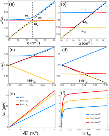
Figure 2: (color online) Magnon-polariton spectrum for $H=0$ (a) and $H=0.15H_{\mathrm{sp}}$ (b), respectively. $N=1.56\times 10^{6}$, $H_{a}=0.016H_{ex}$. The dashed lines refer to the photon mode $\omega=cq$. (c-d) The frequency of the magnon-photon system as a function of external field at given photon frequency $\omega_{c}=1.04\omega_{r}$ and $0.96\omega_{r}$, respectively. when the external fields is adjusted. (e) The band gap of the coupled spectrum $\Delta\omega$ as a function of the number of spins under fields $H=0$, $H=0.1H_{sp}$ and $H=0.3H_{\mathrm{sp}}$, respectively. (f) $\Delta\omega$ as a function of the external fields for $N=1.2\times 10^{6}$, $N=1.5\times 10^{6}$ and $N=1.8\times 10^{6}$, respectively. Other parameters are $H_{\mathrm{ex}}=54$ T, $S=1$, $V=1\ \mathrm{mm^{3}}$, $a=0.4$ nm.

The transmission of an incident EM wave is often measured in the experiments. As argued in the previous publications Harder2016 , the transmission can be viewed as a scattering process, which is well described by the Green function of a magnet-light system. Suppose the eigenvectors of eigenvalues $\omega_{1,2,3}$ are $\left|1\right>,\left|2\right>,\left|3\right>$, respectively. Then the Green function in the diagonal basis is

$$G=\sum_{k=1,2,3}\frac{\left|k\right>\left<k\right|}{\omega-\omega_{k}+i\epsilon}$$ (9)

where $\epsilon$ is an arbitrary small positive number. The transmission amplitude is the imaginary part of the Green function, i.e. $\mathbf{T}(\omega)\propto-\mathrm{Im}(\mathbf{G}(\omega))$. The transmission of an incident wave $\left|\varphi_{0}\right>$ (eigen-mode of $c_{q}^{\dagger}c_{q}$) is $T=\left<\varphi_{0}\right|\mathbf{T}\left|\varphi_{0}\right>$. Figure 3a is the transmission near the photon frequency for $H=0.15H_{sp}$ and $N=1.56\times 10^{7}$. Two transmission peaks center at the calculated eigen-frequency (dashed lines), which demonstrates the strong magnon-photon coupling. The $\delta$-function like transmission peaks are due to the absence of the damping. In realistic case, the damping will broaden the peaks of the Lorentzian curve. If the damping is large enough, the two Lorentzian peaks will merge to a single peak and then the coupling modes cannot be identified.

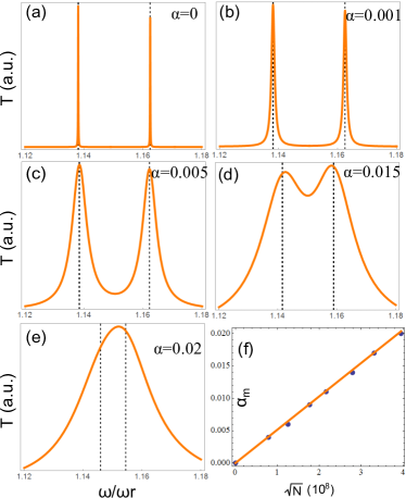
Figure 3: (color online) Transmission of incident wave at $\alpha=0$ (a), 0.001 (b), 0.005 (c), 0.015 (d) and 0.02 (e) for $H=0.15H_{\mathrm{sp}}$. The vertical dashed lines indicate the positions of the coupled modes. (f) The $\sqrt{N}-$dependence of maximum damping that can have two distinguishable resonance peaks for $H=0.15H_{\mathrm{sp}}$. The linear line is $\alpha_{m}=\Delta\omega/\sqrt{2}\omega_{c}$, where $\Delta\omega$ is proportional to $\sqrt{N}$.

To quantitatively see the influence of damping on the transmission spectrum, we first replace $\omega_{r}$ by $\omega_{r}-i\alpha\omega_{r}$ in the matrix $\mathbf{M}$, where $\alpha$ is the strength of damping, then we calculate the complex eigenvalues and eigenvectors of $\mathbf{M}$ and use them to compute the imaginary part of the Green function (transmission amplitude). Figure 3b-e is the frequency-dependence of the transmission for $\alpha$ increasing from 0.001 to 0.02. Indeed, (transmission) peak width increases, and peak height decreases with the increase of $\alpha$. For the parameters used in our calculations, two peaks become indistinguishable for damping larger than 0.02. As the number of spins $N$ increases, the coupling strength between magnons and photons increases, then the magnon-polariton is more stable to resist the intrinsic damping of magnons. Figure 3f shows the maximum damping $\alpha_{m}$ that allows clear identification of the two coupled modes as a function of $\sqrt{N}$ for $H=0.15H_{sp}$, which verifies the argument. Quantitatively, the linewidth of the absorption curve should be $c_{0}\alpha\omega_{c}$, then the maximum damping could be derived as $c_{0}\alpha_{m}\omega_{c}=\Delta\omega$ i.e. $\alpha_{m}=\Delta\omega/(c_{0}\omega_{c})$. The numerical data could be perfectly described by using $c_{0}=\sqrt{2}$, as shown by the orange line in Fig. 3f.

Our results suggest that the key to realize the strong magnon-photon coupling in AFMs is to use low damping materials. The intrinsic damping of an antiferromagnetic metal is of the order of 0.5 according to the first principles calculation, which will be published elsewhere. Hence antiferromagnetic metals are not favorable for realizing strong magnon-photon coupling. The damping of antiferromagnetic insulators such as NiO can be as low as $2.1\times 10^{-4}$ Kampfrath2011 , comparable to that of YIG. Thus, the strong coupling can be realized in low damping antiferromagnetic insulators according to our results. In terms of the detection of the coupling signal, we can either measure the transmission spectrum or use electric detection method to measure the voltage signal of a hybridized structure. For the ferromagnetic case, the coupling strength between magnon and microwave photons have been measured through the electrical detection of spin pumping from the ferromagnetic layer Flaig2016 . It was recently reported that spin pumping exists also at the interface of AFM/normal metal Cheng2014 . In fact, AFM layer may even enhance the spin pumping. Thus, electrical detection of the coupling signal in AFM is also possible in the hybridized structures. Furthermore, magnon modes in an AFM has already been experimentally excited by using sub-THz technology Caspers2016 .

In conclusions, we have quantum-mechanically investigated the magnon-photon coupling in an antiferromagnet. The coupling strength is proportional to the square root of number of spins and can be order of several $\mu eV$ to tens of $\mu eV$, which could be observed in low damping AFM insulators. In the absence of an external field, only one magnon band is coupled with the cavity photon and anticrosses with each other near the cavity frequency while the other does not. External fields remove the double degeneracy in magnon bands and both magnon bands couple to the cavity photon, resulting in two anticrossings.

HYY would like to thank Ke Xia, Zhe Yuan, Grigoryan Vahram and Meng Xiao for helpful discussions. XRW acknowledges the support from National Natural Science Foundation of China (Grant No. 11374249) and Hong Kong RGC (Grant No. 163011151 and 16301816).

References

- (1) K. B. Tolpygo, Zh. Eksp. Teor. Fiz. 20, 497 (1950).
- (2) K. Huang, Nature 167, 779 (1951).
- (3) R. H. Ritchie, Phys. Rev. 106, 874 (1957).
- (4) W. L. Barnes, A. Dereux, and T. W. Ebbesen, Nature 424, 824 (2003).
- (5) P. Berini and I. De Leon, Nat. Photon. 6, 16 (2011).
- (6) A. Wallraff, D. I. Schuster, A. Blais, L. Frunzio, R.-S. Huang, J. Majer, S. Kumar, S. M. Girvin, and J. Schoekopf, Nature 431, 162 (2004).
- (7) S. Dufferwiel, S. Schwarz, F. Withers, A. A. P. Trichet, F. Li, M. Sich, O. Del Pozo-Zamudio, C. Clark, A. Nalitov, D. D. Solnyshkov, G. Malpuech, K. S. Novoselov, J. M. Smith, M.S. Skolnick, D. N. Krizhanovskii, and A. I. Tartakovskii, Nat. Commun. 6, 8579 (2015).
- (8) Ö. O. Soykal and M. E. Flatté, Phys. Rev. Lett. 104, 077202 (2010).
- (9) H. Huebl, C. W. Zollitsch, J. Lotze, F. Hocke, M. Greifenstein, A. Marx, R. Gross, and S. T. B. Goennenwein, Phys. Rev. Lett. 111, 127003 (2013).
- (10) Y. Cao, P. Yan, H. Huebl, S. T. B. Goennenwein, and G. E. W. Bauer, Phys. Rev. B 91, 094423 (2015).
- (11) P. Yan, X. S. Wang, and X. R. Wang, Phys. Rev. Lett. 107, 177207 (2011).
- (12) X. S. Wang, P. Yan, Y. H. Shen, G. E. W. Bauer, and X. R. Wang, Phys. Rev. Lett. 109, 167209 (2012).
- (13) B. Hu and X. R. Wang, Phys. Rev. Lett. 111, 027205 (2013).
- (14) H. Walther, B. T. H. Varcoe, B. Englert, and T. Becker, Rep. Prog. Phys. 69, 1325 (2006).
- (15) Y. Tabuchi, S. Ishino, T. Ishikawa, R. Yamazaki, K. Usami, and Y. Nakamura, Phys. Rev. Lett. 113, 083603 (2014).
- (16) X. Zhang, C.-L. Zou, L. Jiang, and H. X. Tang, Phys. Rev. Lett. 113, 156401 (2014).
- (17) L. Bai, M. Harder, Y. P. Chen, X. Fan, J. Q. Xiao, and C. -M. Hu, Phys. Rev. Lett. 114, 227201 (2015).
- (18) H. Maier-Flaig, M. Harder, R. Gross, H. Huebl, S. T. B. Geennenwein, arXiv:1601.05681v1
- (19) T. Jungwirth, X. Marti, P. Wadley, and J. Wunderlich, Nat. Nanotech. 11, 231 (2016).
- (20) C. Manohar and G. Venkataraman, Phys. Rev. B 5, 1993 (1972).
- (21) S. M. Bose, E-Ni. Foo, and M. A. Zuniga, Phys. Rev. B 12, 3855 (1975).
- (22) T. Holstein and H. Primakoff, Phys. Rev. 58, 1098 (1940).
- (23) M. Harder, L. Bai, C. Match, J. Sirker, and C. -M. Hu, arXiv:1601.06049v2.
- (24) T. Kampfrath, A. Sell, G. Klatt, A. Pashkin, S. Mährlein, T. Dekorsy, M. Wolf, M. Fiebig, A. Leitenstorfer, and R. Huber, Nat. Photon. 5, 31 (2011).
- (25) R. Cheng, J. Xiao, Q. Liu, and A. Brataas, Phys. Rev. Lett. 113 057601 (2014).
- (26) C. Caspers, V. P. Gandhi, A. Magrez, E. de Rijk, and Jean-Philippe Ansermet, Appl. Phys. Lett. 108, 241109 (2016).