Ionic vibration induced transparency and Autler-Townes splitting

Abstract

In this work, the absorption spectrum of a two-level ion in a linear Paul trap is investigated, the ion is supposed to be driven by two orthogonal laser beams, the one along the axial of the trap acts as the control light beam, the other as probe beam. When the frequency of the control laser is tuned to the first red sideband of the ionic transition, the coupling between the internal states of the ion and vibrational mode turns out to be a Jaynes-Cummings (JC) Hamiltonian, which together with the coupling between the probe beam and the two-level ion constructs a $\Lambda$-type three-level structure. In this case the transparency window may appear in the absorption spectrum of the probe light, which is induced by the ionic vibration and is very similar to the cavity induced transparency [1996 Opt. Commun. 126 230-235]. On the other hand, when the frequency of the control laser is tuned to the first blue sideband of the ionic transition, the two-level ion and vibrational mode are governed by an anti-Jaynes-Cummings (anti-JC) Hamiltonian, the total system including the probe beam forms a $V$-type three-level structure. And the Autler-Townes splitting in the absorption spectrum is found.

I Introduction

Quantum interferences, which may occur in many quantum processes along alternative pathways, play a very significant role in quantum mechanics. The superpositions of the probability amplitudes in different pathways give rise to phenomena analogous to constructive and destructive interference between classical waves. In quantum optics many valuable applications of quantum interferences such as coherent population trapping CPT ; CPT2 , lasing without inversion LWI ; LWI2 and electromagnetically induced transparency (EIT) EIT1 ; EIT2 ; EIT3 have been examined. As for the EIT, it is the quantum interference that makes the transparency of a weak probe light through an originally opaque atomic medium in a narrow spectral window with the help of a strong control laser beam. Electromagnetically induced transparency has been studied extensively and generalized in different ways; several EIT-like phenomena have also been predicted and some of them have been observed experimentally. For instance, Rice and Brecha predicted that, in cavity QED where a single-mode cavity contains a two-level atom, a hole in the absorption spectrum of the atom may emerge at line center for a weak probe light, this phenomenon is exactly due to the quantum interference between two different transition paths induced by the cavity field, and it is called cavity induced transparency (CIT) CIT . It was shown that the vacuum Rabi splitting in a cavity QED can even induce the transparency of a probe light in the $\Lambda$-type three-level system, called vaccum induced transparency VaIT0 ; VaIT . In a cavity-optomechanical system COM , the optomechanically induced transparency was realized in experiment OMIT1 ; OMIT2 , in which an optical light, tuned to a sideband transition of a micro-optomechanical system, acts as control field, and the intracavity field acts as a probe field, such a system forms a $\Lambda$-type three-level structure, and the presence of the control field can thus induce the transparency of the probe field. Electromagnetically induced transparency and EIT-like phenomena have many potential applications in controlling the propagation properties of the medium for light such as absorption coefficient, refractive index, propagating speed and nonlinearity etc. Lukin , and in quantum information processing such as quantum information memory Polariton .

Besides, a phenomenon similar to EIT, known as Autler-Townes splitting (ATS) ATS1 ; ATS2 ; ATS3 , also displays a dip in the absorption spectrum of a weak probe field in a quantum system appropriately coupling to a strong driving field. Differently, ATS is not contributed to destructive interference but to the driving-field-induced shift of the transition frequency EITATS . Abi-Salloum analyzed three-level systems: $\Lambda$, $V$ and two ladder with upper- and lower-level driving respectively, and found EIT mainly appears in $\Lambda$ and upper-driven ladder three-level systems and ATS in V and lower-driven ladder three-level systems EITATS . Anisimov et al. proposed an objective method on discerning ATS from EIT EA1 .

On the other hand, ion traps have been developed to be a state-of-the-art technique for solving problems in quantum mechanics, quantum optics and quantum information processing etc., for instance, the famous Jaynes-Commings (JC) model and various generalized JC models were realized experimentally for two-level ions and the phonons of the ionic vibration RMP-ion ; the controlled-NOT operation proposed by Cirac and Zoller Cirac-Zoller was realized in experiment as well Cirac-ZollerEXP . Moreover, very recently, high-fidelity trapped-ion-based quantum logic gates iontrapEXP ; Wineland2 and those with multi-element qubits Wineland1 were demonstrated; and Shor’s algorithm Blatt1 and the quantum simulation of lattice gauge theories Blatt2 were realized as the first step towards a real quantum computer.

As trapped ions can provide us a system governed by JC or anti-JC Hamiltonian as cavity QED system does, one may naturally ask the following question whether one can resort to the ionic vibration to realize the transparency of a probe light. In this paper, we give a positive answer to this question. Our results show when the control laser light is tuned to the first red sideband of the ionic transition (corresponding to the JC model), a transparency window in the absorption spectrum of the probe light emerges, we refer to such a phenomenon as ionic vibration induced transparency (VIT). And when the control laser light is tuned to the first blue sideband of the ionic transition (corresponding to the anti-JC model), Autler-Townes splitting emerges, which also displays a dip (or reduction, hole) in the absorption spectrum.

The rest of this paper is organized as follows, in Sec. 2, we describe the theoretical model of our scheme and the Hamiltonian for the driven trapped ion in Lamb-Dicke regime. In Sec. 3 we investigate the VIT when the frequency of the control light is tuned to the first red sideband of the ionic transition; in Sec. 4 we show the ATS when the frequency of the control light is tuned to the first blue sideband of the ionic transition. Finally, we end with discussion and conclusion in Sec. 5.

II Theoretical model

The system we consider here is a single two-level ion confined in a linear Paul trap, where the strength of the radial confinement is assumed to be largely stronger than that along the axial direction, the movement in the radial direction can thus be ignored RMP-ion and one considers only the center-of-mass mode of the ionic vibration. We assume the ion in the Paul trap is driven by two orthogonal laser beams, one is along the axial (or longitudinal) direction of the trap, the other along the radial (or transverse) direction. We further assume the longitudinal laser beam is a traveling wave with frequency $\omega_{L}$ and it acts as the control light beam. The transverse laser beam is a weak laser light with a tunable frequency $\omega_{P}$ and it acts as the probe field.

As the motion of the ion is mainly in the longitudinal direction and the transverse motion can almost be ignored, the Hamiltonian for this system is thus given by RMP-ion

$$H =\frac{\hbar}{2}\omega_{a}\sigma_{z}+\hbar(\nu a^{\dagger}a+\frac{1}{2})+\frac{\hbar}{2}\Omega\left(\sigma_{+}+\sigma_{-}\right)\times$$ (1)

$$\left[e^{i\eta\left(a^{\dagger}+a\right)-i\omega_{L}t}+e^{-i\eta\left(a^{\dagger}+a\right)+i\omega_{L}t}\right]$$

$$+i\hbar\varepsilon\left(\sigma_{-}e^{i\omega_{P}t}-\sigma_{+}e^{-i\omega_{P}t}\right),$$

where $\sigma_{z}=\left|e\right\rangle\left\langle e\right|-$ $\left|g\right\rangle\left\langle g\right|,$ $\sigma_{+}=\left|e\right\rangle\left\langle g\right|,$ and $\sigma_{-}=\left|g\right\rangle\left\langle e\right|$ with $\left|e\right\rangle$ and $\left|g\right\rangle$ being the excited and ground states of the ion respectively, $a^{\dagger}$ and $a$ are the creation and annihilation operators for the center-of-mass motion of the trapped ion respectively, $\Omega$ ( $\varepsilon$ ) is the Rabi frequency of the longitudinal (transverse) laser field, and $\eta=k_{L}/\sqrt{2m\nu}$ is the Lamb-Dicke parameter, with $k_{L}=\omega_{L}/c$ being the wave vector of the longitudinal laser field.

We suppose the trapped ion is constrained in the Lamb-Dicke regime, and the Lamb-Dicke parameter $\eta$ meets the condition $\eta\ll 1$. The Hamiltonian $H$ can be approximated by the expansion to the first order in $\eta$,

$$H \approx\frac{\hbar}{2}\omega_{a}\sigma_{z}+\hbar(\nu a^{\dagger}a+\frac{1}{2})+\frac{\hbar}{2}\Omega\left(\sigma_{+}+\sigma_{-}\right)\times$$ (2)

$$\left[e^{-i\omega_{L}t}\left(1+i\eta a+i\eta a^{\dagger}\right)+e^{i\omega_{L}t}\left(1-i\eta a-i\eta a^{\dagger}\right)\right]$$

$$+i\hbar\varepsilon\left(\sigma_{-}e^{+i\omega_{P}t}-\sigma_{+}e^{-i\omega_{P}t}\right).$$

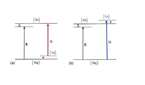
Figure 1: Transition processes in $(a)$ red-detuning case and $(b)$ blue-detuning case.

In the following we will investigate the two different cases in which the frequency of the longitudinal laser beam, $\omega_{L}$, is respectively tuned to the first red sideband or the first blue sideband of the ionic internal transition frequency $\omega_{a}$. In the red-detuning case, when the frequency of the longitudinal laser beam is tuned to the first red sideband of the atomic transition, the frequency of the control light satisfies $\omega_{L}=\omega_{a}-\nu$; we apply a unitary transformation to the Hamiltonian $H\$to deal with the counterrotating-wave terms in Eq. ($2$),

$$H^{\prime}=i\hbar\frac{\partial U_{R}^{\dagger}}{\partial t}U_{R}+U_{R}^{\dagger}HU_{R},$$ (3)

where

$$U_{R}=\exp\left\{-i\left[\frac{1}{2}\omega_{P}\sigma_{z}+\left(\omega_{P}-\omega_{L}\right)a^{\dagger}a\right]t\right\}.$$ (4)

Then the Hamiltonian of the system can be simplified by discarding the rapidly oscillating terms (taking the rotating-wave approximation), and we finally obtain

$$H^{\prime}=H_{JC}+i\hbar\varepsilon\left(\sigma_{-}-\sigma_{+}\right),$$ (5)

where $\Delta=\omega_{a}-\omega_{P}$ is the detuning between the ionic transition and probe field and $H_{JC}$ is the JC Hamiltonian taking the form

$$H_{JC}=\frac{\hbar}{2}\Delta\sigma_{z}+\hbar\Delta a^{\dagger}a+\frac{i\hbar}{2}\eta\Omega\left(\sigma_{+}a-\sigma_{-}a^{\dagger}\right).$$ (6)

In the blue-detuning case, the frequency of the longitudinal laser beam is setted to $\omega_{L}=\omega_{a}+\nu$, that is, the longitudinal laser is tuned to the first blue sideband of the atomic transition. Here we apply the following unitary transformation to the Hamiltonian $H$ (Eq. ($2$)),

$$H^{\prime\prime}=i\hbar\frac{\partial U_{B}^{\dagger}}{\partial t}U_{B}+U_{B}^{\dagger}HU_{B},$$ (7)

where

$$U_{B}=\exp\left\{-i\left[\frac{1}{2}\omega_{P}\sigma_{z}+\left(\omega_{L}-\omega_{P}\right)a^{\dagger}a\right]t\right\}.$$ (8)

Similar to the red-detuning case, we obtain an anti-JC Hamiltonian by utilizing the rotating-wave approximation

$$H^{\prime\prime}=H_{AJC}+i\hbar\varepsilon\left(\sigma_{-}-\sigma_{+}\right),$$ (9)

and the anti-JC Hamiltonian takes the form

$$H_{AJC}=\frac{\hbar}{2}\Delta\sigma_{z}-\hbar\Delta a^{\dagger}a+\frac{i\hbar}{2}\eta\Omega\left(\sigma_{+}a^{\dagger}-\sigma_{-}a\right).$$ (10)

If we concentrate on the case that the motion of the ion is nearly confined to its ground state and the probe light is very weak, only the zero- and one-phonon states of the vibration of the ion need to be taken into account. Following Ref. CIT the total states of the system in the red-detuning case are now spanned by $\{\left|0g\right\rangle,$ $\left|0e\right\rangle,$ $\left|1g\right\rangle\}$, where $\left|0g\right\rangle\equiv\left|0\right\rangle\otimes\left|g\right\rangle$ and so on, here the numerical index, $0$ or $1$, indicates the phonon number state. The energy level structure of these three states is sketched in Fig. $1(a)$. Similarly, in the blue-detuning case the total states of the system are spanned by $\mathbf{\{}\left|0g\right\rangle,$ $\left|0e\right\rangle,$ $\left|1e\right\rangle\}$. The energy level structure in this case is sketched in Fig. $1(b)$.

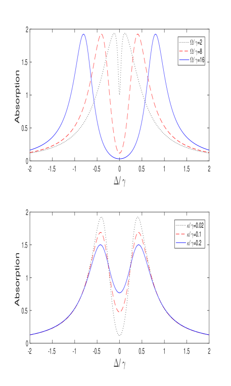
Figure 2: The absorption spectra for the probe light when the control light is tuned to the first red sideband. The vertical axis is $Im[\rho_{0g;0e}/i\varepsilon]$ in the unit of $1/\gamma$ and the horizontal axis is $\Delta/\gamma$ with the Lamb-Dicke parameter $\eta=0.1$. $(a)$ $\gamma/\kappa=50$ and $\Omega/\gamma=2$ (black dotted line), $\Omega/\gamma=8$ (red dashed line), $\Omega/\gamma=16$ (blue solid line). $(b)$ $\Omega/\gamma=8$ and $\kappa/\gamma=0.02$ (black dotted line), $\kappa/\gamma=0.1$ (red dashed line), $\kappa/\gamma=0.2$ (blue solid line).

III VIT in red-detuning case

Now let us consider the spontaneous emission of the ionic excited state and the heating effect of the vibrational motion induced by coupling to the environment. We suppose the interaction between the ionic internal states and its reservoir is weak, so is the interaction between the vibrational mode and its reservoir. Thus one can adopt the Born and Markov approximations to deal with spontaneous emission and the heating effect, and the master equation for such a system takes the form

$$\dot{\rho} = -\frac{i}{\hbar}\left[H^{\prime},\rho\right]+\kappa(\overline{n}+1)\left(2a\rho a^{\dagger}-a^{\dagger}a\rho-\rho a^{\dagger}a\right)$$ (11)

$$+\kappa\overline{n}\left(2a^{\dagger}\rho a-aa^{\dagger}\rho-\rho aa^{\dagger}\right)$$

$$+\frac{\gamma}{2}\left(2\sigma_{-}\rho\sigma_{+}-\sigma_{+}\sigma_{-}\rho-\rho\sigma_{+}\sigma_{-}\right),$$

where $\kappa$ is the heating rate for vibrational motion and $\overline{n}$ is the average thermal phonon number, $\gamma$ is the spontaneous emission rate, here we have assumed that the ionic excited state couples to the vacuum reservoir of the electromagnetic field. As supposed above, the vibration of the ion is nearly confined to its ground state, so the average thermal phonon $\overline{n}$ is almost zero.

The elements of the density matrix in the states $\{\left|0g\right\rangle,$ $\left|0e\right\rangle,$ $\left|1g\right\rangle\}$ take the following form according to the master equation ($11$):

$$\dot{\rho}_{0g;0g} = \gamma\rho_{0e;0e}+2\kappa\rho_{1g;1g}+\varepsilon\left(\rho_{0e;0g}+\rho_{0g;0e}\right),$$ (12)

$$\dot{\rho}_{0g;0e} = \left(i\Delta-\frac{\gamma}{2}\right)\rho_{0g;0e}+\frac{\eta\Omega}{2}\rho_{0g;1g}$$ (13)

$$-\varepsilon\left(\rho_{0g;0g}-\rho_{0e;0e}\right),$$

$$\dot{\rho}_{0g;1g} = \left(i\Delta-\kappa\right)\rho_{0g;1g}-\frac{\eta\Omega}{2}\rho_{0g;0e}+\varepsilon\rho_{0e;1g},$$ (14)

$$\dot{\rho}_{0e;0e} = -\gamma\rho_{0e;0e}+\frac{\eta\Omega}{2}\left(\rho_{0e;1g}+\rho_{1g;0e}\right)$$ (15)

$$-\varepsilon\left(\rho_{0g;0e}+\rho_{0e;0g}\right),$$

$$\dot{\rho}_{0e;1g} = -\left(\kappa+\frac{\gamma}{2}\right)\rho_{0e;1g}-\varepsilon\rho_{0g;1g}$$ (16)

$$+\frac{\eta\Omega}{2}\left(\rho_{1g;1g}-\rho_{0e;0e}\right),$$

$$\dot{\rho}_{1g;1g} = -2\kappa\rho_{1g;1g}-\frac{\eta\Omega}{2}\left(\rho_{0e;1g}+\rho_{1g;0e}\right).$$ (17)

We suppose both the internal state and the vibrational mode of the motion of the ion are initially in their ground state, $\left|0g\right\rangle,$ that is, $\rho_{0g;0g}(0)=1,\rho_{0e;0e}(0)=\rho_{1g;1g}(0)=\rho_{0e;1g}(0)=0$. In order to examine the prperties of the refraction and the absorption for the probe light, we adopt the expression of the complex susceptibility which is given by $\chi=\chi^{\prime}+i\chi^{\prime\prime}\propto\left(\rho_{0g;0e}/i\varepsilon\right)$ CIT ; Scully ; Meystre , where the real part $\chi^{\prime}$ stands for the index of refraction of the medium and the imaginary part $\chi^{\prime\prime}$ is proportional to the absorption coefficient. Hence our task is to solve the equations about the elements of the density matrix in order to obtain $\rho_{0g;0e}$. For simplicity, in the following we only focus on the steady-state solution of the elements of the density matrix by setting their first derivatives with respect to time to zero. We finally get the steady-state solution to $\rho_{0g;0e}$ and hence yielding the information about the absorption coefficient $\chi^{\prime\prime}$ and dispersion coefficient $\chi^{\prime}$ of a weak probe field. This is given by

$$\rho_{0g;0e}=\frac{\varepsilon\left(i\Delta-\kappa\right)}{\left(i\Delta-\frac{\gamma}{2}\right)\left(i\Delta-\kappa\right)+\left(\frac{\eta\Omega}{2}\right)^{2}}.$$ (18)

The numerical results of $Im[\rho_{0g;0e}/i\varepsilon]$ are given in Fig. $2$, which shows there exists VIT for the probe light when its frequency is close to the ionic transition frequency. Figure $2(a)$ indicates that the transparency window becomes wider and deeper as $\Omega$ is getting larger if the other parameters are unchanged. Figure $2(b)$ shows that as the heating rate $\kappa$ increases the depth of transparency window becomes shallow, which indicates the heating effect makes the system more opaque.

IV ATS in blue-detuning case

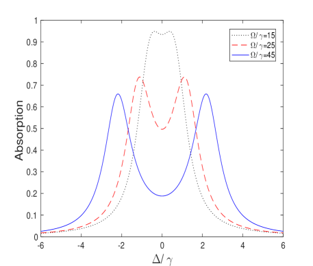
Figure 3: The absorption spectra for the probe light when the control light is tuned to the first blue sideband. The vertical axis is $Im[\rho_{0g;0e}/i\varepsilon]$ in the unit of $1/\gamma$ and the horizontal axis is $\Delta/\gamma$ with the Lamb-Dicke parameter $\eta=0.1$, $\gamma/\kappa=50$ and $\Omega/\gamma=15$ (black dotted line), $\Omega/\gamma=25$ (red dashed line), $\Omega/\gamma=45$ (blue solid line).

The master equation for the blue-detuning case can be derived by the way similar to the red-detuning case and it takes the following form

$$\dot{\rho} = -\frac{i}{\hbar}\left[H^{\prime\prime},\rho\right]+\kappa(\overline{n}+1)\left(2a^{\dagger}\rho a-aa^{\dagger}\rho-\rho aa^{\dagger}\right)$$ (19)

$$+\kappa\overline{n}\left(2a\rho a^{\dagger}-a^{\dagger}a\rho-\rho a^{\dagger}a\right)$$

$$+\frac{\gamma}{2}\left(2\sigma_{-}\rho\sigma_{+}-\sigma_{+}\sigma_{-}\rho-\rho\sigma_{+}\sigma_{-}\right).$$

Because the ionic vibration is supposed to be confined to its ground state, the average thermal phonon $\overline{n}$ is almost zero and the motion of the ion is mostly in the zero- or one-phonon state. According to the master equation, the elements of the density matrix in the states $\{\left|0g\right\rangle,$ $\left|0e\right\rangle,$ $\left|1e\right\rangle\}$ are of the form:

$$\dot{\rho}_{0g;0g} = -2\kappa\rho_{0g;0g}-\frac{\eta\Omega}{2}\left(\rho_{0g;1e}+\rho_{1e;0g}\right)$$ (20)

$$+\varepsilon\left(\rho_{0e;0g}+\rho_{0g;0e}\right)+\gamma\rho_{0e;0e},$$

$$\dot{\rho}_{0g;0e} = \left(i\Delta-2\kappa-\frac{\gamma}{2}\right)\rho_{0g;0e}-\frac{\eta\Omega}{2}\rho_{1e;0e}$$ (21)

$$-\varepsilon\left(\rho_{0g;0g}-\rho_{0e;0e}\right),$$

$$\dot{\rho}_{1e;0g} = -\left(3\kappa+\frac{\gamma}{2}\right)\rho_{1e;0g}+\varepsilon\rho_{1e;0e}$$ (22)

$$+\frac{\eta\Omega}{2}\left(\rho_{0g;0g}-\rho_{1e;1e}\right),$$

$$\dot{\rho}_{1e;0e} = \left(i\Delta-3\kappa-\gamma\right)\rho_{1e;0e}+\frac{\eta\Omega}{2}\rho_{0g;0e}-\varepsilon\rho_{1e;0g},$$ (23)

$$\dot{\rho}_{0e;0e} = -\left(2\kappa+\gamma\right)\rho_{0e;0e}-\varepsilon\left(\rho_{0g;0e}+\rho_{0e;0g}\right),$$ (24)

$$\dot{\rho}_{1e;1e} = -\left(4\kappa+\gamma\right)\rho_{1e;1e}+2\kappa\rho_{0e;0e}$$ (25)

$$+\frac{\eta\Omega}{2}\left(\rho_{0g;1e}+\rho_{1e;0g}\right).$$

In the same way, the susceptibility is given by $\chi=\chi^{\prime}+i\chi^{\prime\prime}\propto\left(\rho_{0g;0e}/i\varepsilon\right)$, $\chi^{\prime}$ and $\chi^{\prime\prime}$ are related to the refraction of the medium and the absorption coefficient, respectively.

As done in Sec. III, the steady-state solution to $\rho_{0g;0e}$ can be derived by setting the derivatives of the elements of the density matrix in Eqs. ($20-25$) to zero in the initial condition of $\rho_{0e;0e}(0)=1,\rho_{0g;0g}(0)=\rho_{1e;1e}(0)=\rho_{1e;0g}(0)=0$. Thus the solution to $\rho_{0g;0e}$ is

$$\rho_{0g;0e}=\frac{\varepsilon\left(i\Delta-3\kappa-\gamma\right)}{\left(i\Delta-2\kappa-\frac{\gamma}{2}\right)\left(i\Delta-3\kappa-\gamma\right)+\left(\frac{\eta\Omega}{2}\right)^{2}}.$$ (26)

In Fig. $3$ we plot the numerical result of $Im[\rho_{0g;0e}/i\varepsilon]$ as the function of $\Delta/\gamma$. Similar to the red-detuning case, a dip in absorption spectrum of the probe light emerges slowly in such a case. It is obvious that the dip becomes deeper and wider with the increase of $\Omega$ under the condition of the other parameters unchanged.

V Discussion and conclusion

The absorption spectra of the probe light in both cases of red-detuning and blue-detuning are investigated, and a dip in the spectrum can emerge in both cases. Differently, in the red-detuning case, the energy level configration is of $\Lambda$-type three structure and the dip in absorption spectrum exhibits the properties of EIT, that is, a narrow and deep dip can appear when the driving light is not so strong, while in the blue-detuning case, the energy level configration takes $V$-type three structure and the dip exhibits the properties of ATS, the appearance of the dip requires a stronger driving light and the dip is either narrow but shallow or deep but wide, i.e., the dip cannot be narrow and deep at the same situation.

Our proposal about the VIT may be verified experimentally. On the one hand, the techniques for ion traps have been utilized to realize much complicated quantum process RMP-ion and quantum logic gates Cirac-ZollerEXP ; iontrapEXP ; Wineland2 ; Wineland1 as mentioned in Sec. I, such techniques pave a way for the VIT and ATS presented here. On the other hand, vaccum induced transparency in a cavity VaIT indicates that the transparency of light can be achieved for several or even a single atom(s), thus our proposal should be realized experimentally.

To summarize, in the present work we have investigated ionic vibration induced transparency and Autler-Townes splitting in a linear Paul trap. When control light is tuned to the first red sideband of the ionic transition, the VIT emerges and it is very similar to the CIT CIT . When the control light is tuned to the first blue sideband of the ionic transition, the ATS emerges via anti-JC Hamiltonian. We find in both cases the dip in the absorption spectra becomes wider and deeper as the Rabi frequency of the control light increases.

References

- (1) G. Alzetta, A. Gozzini, L. Moi, and G. Orriols, An experimental method for the observation of r.f. transitions and laser beat resonances in oriented Na vapour, Nuovo Cimento Soc. Ital. Fis., B 36, 5 (1976).
- (2) R. M. Whitley and C. R. Stroud, Jr., Double optical resonance, Phys. Rev. A 14, 1498 (1976).
- (3) S. E. Harris, Lasers without inversion: Interference of lifetime-broadened resonances, Phys. Rev. Lett. 62, 1033 (1989).
- (4) M. O. Scully, S.-Y. Zhu, and A. Gavrielides, Degenerate quantum-beat laser: Lasing without inversion and inversion without lasing, Phys. Rev. Lett. 62, 2813 (1989).
- (5) S. E. Harris, J. E. Field, and A. Imamoğlu, Nonlinear optical processes using electromagnetically induced transparency, Phys. Rev. Lett. 64, 1107 (1990).
- (6) M. Fleischhauer, A. Imamoglu, and J. P. Marangos, Electromagnetically induced transparency: Optics in coherent media, Rev. Mod. Phys. 77, 633 (2005).
- (7) K.-J. Boller, A. Imamolu, and S. Harris, Observation of electromagnetically induced transparency, Phys. Rev. Lett. 66, 2593 (1991).
- (8) P. R. Rice, R. J. Brecha, Cavity induced transparency, Opt. Comm. 126, 230 (1996).
- (9) J. E. Field, Vacuum-Rabi-splitting-induced transparency, Phys. Rev. A 47, 5064 (1993).
- (10) H. Tanji-Suzuki, W. Chen, R. Landig, J. Simon, V. Vuletić, Vacuum-induced transparency, Science 333, 1266 (2011).
- (11) M. Aspelmeyer, T. J. Kippenberg, F. Marquardt, Cavity optomechanics, Rev. Mod. Phys. 86, 1391 (2013).
- (12) A. Schliesser, Optomechanically induced transparency, Science 330, 1520 (2010).
- (13) P.-C. Ma, J.-Q. Zhang, Y. X., M. Feng, and Z.-M. Zhang, Tunable double optomechanically induced transparency in an optomechanical system, Phys. Rev. A 90, 043825 (2014).
- (14) M. D. Lukin, Colloquium: Trapping and manipulating photon states in atomic ensembles, Rev. Mod. Phys. 75, 457 (2003).
- (15) M. Fleischhauer and M. D. Lukin, Dark-state polaritons in electromagnetically induced transparency, Phys. Rev. Lett. 84, 5094 (2000).
- (16) S. H. Autler and C. H. Townes, Stark Effect in Rapidly Varying Fields, Phys. Rev. 100, 703 (1955).
- (17) R. Shimano, M. Kuwata-Gonokami, Observation of Autler-Townes Splitting of Biexcitons in CuCl, Phys. Rev. Lett. 72, 530 (1994).
- (18) S. Novikov, J. E. Robinson, Z. K. Keane, et al., Autler-Townes splitting in a three-dimensional transmon superconducting qubit, Phys. Rev. B 88, 060503(R) (2013).
- (19) T. Y. Abi-Salloum, Electromagnetically induced transparency and Autler-Townes splitting: Two similar but distinct phenomena in two categories of three-level atomic systems, Phys. Rev. A 81, 053836 (2010).
- (20) P. M. Anisimov, J. P. Dowling, B. C. Sanders, Objectively discerning Autler-Townes splitting from electromagnetically induced transparency, Phys. Rev. Lett. 107, 163604 (2011).
- (21) D. Leibfried, R. Blatt, C. Monroe, and D. Wineland, Quantum dynamics of single trapped ions, Rev. Mod. Phys. 75, 281 (2003).
- (22) J. I. Cirac, and P. Zoller, Quantum computations with cold trapped ions, Phys. Rev. Lett. 74, 4091 (1995).
- (23) F. Schmidt-Kaler, H. Haffner, M. Riebe et. al., Realization of the Cirac–Zoller controlled-NOT quantum gate, Nature 422, 408 (2003).
- (24) C. J. Ballance, T. P. Harty, N. M. Linke, M. A. Sepiol, and D. M. Lucas, High-fidelity quantum logic gates using trapped-ion hyperfine qubits, Phys. Rev. Lett. 117, 060504 (2016).
- (25) J. Gaebler, T. Tan, Y. Lin, Y. Wan, R. Bowler, A. Keith, S. Glancy, K. Coakley, E. Knill, D. Leibfried, and D. Wineland, High-Fidelity Universal Gate Set for 9Be+ Ion Qubits, Phys. Rev. Lett. 117, 060505 (2016).
- (26) T. R. Tan, J. P Gaebler, Y. Lin, Y. Wan, R. Bowler, D. Leibfried, and D. J. Wineland, Multi-element logic gates for trapped-ion qubits, Nature 528, 380 (2015).
- (27) T. Monz, D. Nigg, E. A. Martinez, M. F. Brandl, P. Schindler, R. Rines, S. X. Wang, I. L. Chuang, R. Blatt, Realization of a scalable Shor algorithm, Science 351, 1068 (2016).
- (28) E. A. Martinez, C. A. Muschik, P. Schindler, D. Nigg, A. Erhard, M. Heyl, P. Hauke, M. Dalmonte, T. Monz, P. Zoller, R. Blatt, Real-time dynamics of lattice gauge theories with a few-qubit quantum computer, Nature 534, 516 (2016).
- (29) Marlan O. Scully, M. Suhail Zubairy, Quantum Optics, chapter 7, p226 (1997).
- (30) Pierre Meystre, Murray Sargent III, Elements of quantum optics, chapter 9, p245 (2007).