Distributed Frequency Control with Operational Constraints, Part I: Per-Node Power Balance

Abstract

This paper addresses the distributed optimal frequency control of multi-area power system with operational constraints, including the regulation capacity of individual control area and the power limits on tie-lines. Both generators and controllable loads are utilized to recover nominal frequencies while minimizing regulation cost. We study two control modes: the per-node balance mode and the network balance mode. In Part I of the paper, we only consider the per-node balance case, where we derive a completely decentralized strategy without the need for communication between control areas. It can adapt to unknown load disturbance. The tie-line powers are restored after load disturbance, while the regulation capacity constraints are satisfied both at equilibrium and during transient. We show that the closed-loop systems with the proposed control strategies carry out primal-dual updates for solving the associated centralized frequency optimization problems. We further prove the closed-loop systems are asymptotically stable and converge to the unique optimal solution of the centralized frequency optimization problems and their duals. Finally, we present simulation results to demonstrate the effectiveness of our design. In Part II of the paper, we address the network power balance case, where transmission congestions are managed continuously.

I Introduction

In a modern large-scale power system, multiple regional grids are usually interconnected for improving operation reliability and economic efficiency [1, 2]. In each control area, power generation and controllable load can be utilized to eliminate power imbalance and maintain frequency stability in real time. Generally, frequency control is a paid service, and hence control areas always try to minimize their control cost. As different control areas may belong to different utilities and global information may not be accessible due to privacy and operational considerations, a distributed strategy is desirable. Roughly speaking, there are two possible modes of operation. In the first mode, each node area balances its own supply and demand after a disturbance. Then the power flow on each tie line should be regulated to its scheduled value, i.e., the deviation of power flows on the tie lines are eliminated in equilibrium. In the second mode, all nodes cooperate to rebalance power over the entire network after a disturbance. The power flows on the tie lines may deviate from their scheduled values but must satisfy line limits in equilibrium. We refer to the first case as per-node (power) balance and the second network (power) balance. Here we focus on the first case, while the second case will be addressed in Part II of the paper. We design a decentralized optimal frequency controller for restoring frequency and tie-lime power under operational constraints, including regulation capacity constraints.

Different distributed strategies have been developed in the literature for frequency control. They can roughly be divided into two categories in terms of different types of regulation resources: the automatic generation control (AGC) e.g. [3, 4, 5, 6, 7, 8, 9] and the load-side frequency control e.g.[10, 11, 12, 13, 14, 15, 16]. The former focuses on generation regulation. For example in [4] a flatness-based control combining trajectory generation and trajectory tracking is proposed for AGC in multi-area power system. In [5, 7], the closed-loop system composed of power system dynamics and controller dynamics is formulated as a port-Hamiltonian system, and its stability is proved. In [6], generators are driven by AGC to restore frequencies. Correspondence between the (partial) primal-dual gradient algorithm for solving the associated optimization problem and the frequency control dynamics of the physical system is established. The resulting decomposition enables the system design of a fully distributed optimal frequency control.

For the load-side frequency control, load frequency dynamics are formulated similarly to the generator model in [10], leading to a distributed frequency control for both generation and controllable loads. A distributed adaptive control is presented in [11] to guarantee acceptable frequency deviation from the nominal value. In [12, 13], an optimal load control (OLC) problem is formulated and a ubiquitous primary load-side control is derived as a partial primal-dual gradient algorithm for solving the OLC problem. It is decentralized, but does not restore the nominal frequency. This design approach is extended in [14] to secondary control that restores nominal frequency and scheduled inter-area flows as well as enforcing line limits in equilibrium. It is further extended to more general models in [15, 16], where passivity condition guaranteeing stability is proposed for each local bus and the conservativeness is reduced greatly.

In terms of methodology, there are mainly three types of distributed frequency control: the droop based approach e.g. [17, 18], the consensus based approach e.g. [19, 20, 21] and the primal-dual decomposition based approach e.g.[12, 13, 14, 6]. In the primal-dual decomposition approach, control goals such as rebalancing power after a disturbance and restoring nominal frequency and scheduled inter-area flows are formalized as a global optimization problem. The feedback control laws are designed so that the equilibrium of the closed-loop system solves the optimization problem and hence achieves the control objectives, in equilibrium. Moreover the closed-loop system is designed to be an asymptotically stable primal-dual algorithm for solving an associated optimization problem. This is the same approach taken in [22] where the real-time control is through nodal proces.

In all the primal-dual algorithms proposed in the literature, even though input constraints are usually enforced, constraints on states, such as power injections on buses, are enforced only in the steady-state. In practice, however, a control area always maintains regulation capacity bounds that constrain power generations and controllable loads within available ranges, not only at equilibrium but also during transient. In this paper, we design input-saturation controllers that maintain these capacity constraints during transient as well. We show that these controllers still carry out primal-dual updates of the associated optimization problem.

Specifically we study an approach to rebalancing power after a disturbance. In the per-node power balance case, we require the disturbance in each control area be balanced by generations and controllable loads in that area. Then we construct a completely decentralized control to recover nominal frequencies and tie-line power flows. The regulation capacity constraints are also enforced during transient. We show that the controller together with the physical dynamics serve as primal-dual updates with saturation for solving the optimization problem. Then we prove the optimality of our control by exploiting the equivalence between the equilibrium of the closed-loop frequency control system and the optimal solution of the optimization problem. We also show that the optimal solution of the primal-dual problem and equilibrium point of the closed-loop systems are both unique. Furthermore we prove the stability of closed-loop system by combining projection technique with LaSalle’s invariance principle, mitigating the impact of nonsmooth dynamics created by the imposed transient constraints. The salient features of our control are:

1. Control goals: the controller restores the nominal frequency and tie-line powers after unknown disturbance while minimizing the regulation costs;

2. Constraints: the regulation capacity constraints are always enforced even during transient;

3. Communication: it is completely decentralized without the need for communication among neighboring areas ;

4. Measurement: the controls are adaptive to unknown load disturbances automatically without load measurement.

The rest of this paper is organized as follows. In Section II, we introduce our network model. Section III formulates the optimal frequency control problem, presents our controller and its relationship with the primal-dual update, and proves the optimality, uniqueness, and stability of the closed-loop equilibrium point. We confirm the performance of controllers via simulations on a detailed power system model in Section IV. Section V concludes the paper.

II Network model

A large power network is usually composed of multiple control areas each with its own generators and loads. These control areas are interconnected with each other through tie lines. For simplicity, here we treat each control area as a node with an aggregate power generation, an aggregate controllable load and an aggregate uncontrollable load. Then the power network is model by a graph ${G}:=(N,E)$ where $N=\{0,1,2,...n\}$ is the set of nodes (control areas) and $E\subseteq N\times N$ is the set of edges (tie lines). If a pair of nodes $i$ and $j$ are connected by a tie line directly, we denote the tie line by $(i,j)\in E$. Let $m:=|E|$ denote the number of tie lines. We treat $G$ as directed with an arbitrary orientation and we use $(i,j)\in E$ or $i\rightarrow j$ interchangeably to denote a directed edge from $i$ to $j$. It should be clear from the context which is the case. Without loss of generality, we assume the graph is connected and node $0$ is a reference node.

For each node $j\in N$, let $\theta_{j}(t)$ denote the rotor angle at node $j$ at time $t$ and $\omega_{j}(t)$ the frequency. Let $P_{j}^{g}(t)$ denote the (aggregate) generation at node $j$ at time $t$ and $u^{g}_{j}(t)$ its generation control command. Let $P^{l}_{j}(t)$ denote the (aggregate) controllable load and $u^{l}_{j}(t)$ its load control command. Let $p_{j}$ denote the (aggregate) uncontrollable load.

We adopt a second-order linearized model to describe the frequency dynamics of each node, and two first-order inertia equations to describe the dynamics of power generation regulation and load regulation at each node. We assume the tie lines are lossless and adopt the DC power flow model. Then for each node $j\in N$,

$$\dot{\theta}_{j} =\omega_{j}(t)$$ (1a)

$$M_{j}\dot{\omega}_{j} =P^{g}_{j}(t)-P^{l}_{j}(t)-p_{j}-D_{j}\omega_{j}(t)$$

$$+\sum_{i:i\rightarrow j}\!B_{ij}(\theta_{i}(t)-\theta_{j}(t))-\sum_{k:j\rightarrow k}\!B_{jk}(\theta_{j}(t)-\theta_{k}(t))$$ (1b)

$$T^{g}_{j}\dot{P}^{g}_{j} =-P^{g}_{j}(t)+u^{g}_{j}(t)-{\omega_{j}(t)}/{R_{j}}$$ (1c)

$$T^{l}_{j}\dot{P}^{l}_{j} =-P^{l}_{j}(t)+u^{l}_{j}(t)$$ (1d)

where $$D_{j}>0 R_{j}>0 B_{jk}>0 (j,k) x:=(\theta,\omega,P^{g},P^{l}) u:=(u^{g},u^{l})$$ are damping constants, are droop parameters, and are line parameters that depend on the reactance of the line . Let denote the state of the network and denote the control.

Our goal is to design feedback control laws for the generation command $u^{g}(x(t))$ and load control $u^{l}(x(t))$. The operational constraints are:

$$\underline{P}^{g}_{j} \leq\ P^{g}_{j}(t)\ \leq\overline{P}^{g}_{j},\quad j\in N$$ (2a)

$$\underline{P}^{l}_{j} \leq\ P^{l}_{j}(t)\ \leq\overline{P}^{l}_{j},\quad j\in N$$ (2b)

Differing from the literature, here (2a) and (2b) are hard limits on the regulation capacities of generation and controllable load at each node, which should not be violated at any time even during transient. Hence we will design controllers so that these constraints are satisfied not only at equilibrium, but also during transient.

We assume that the system operates in a steady state initially, i.e., the generation and the load are balanced and the frequency is at its nominal value. All variables represent deviations from their nominal or scheduled values so that, e.g., $\omega_{j}(t)=0$ means the frequency is at its nominal value.

As the generation $P^{g}_{j}$ and load $P^{l}_{j}$ in each area can increase or decrease, and a line flow $P_{ij}$ can in either direction, we make the following assumption.

• 1. $\underline{P}^{g}_{j}<0<\overline{P}^{g}_{j}$ and $\underline{P}^{l}_{j}<0<\overline{P}^{l}_{j}$ for $\forall j\in N$.

  2. $\theta_{0}(t):=0$ for all $t\geq 0$.

The assumption $\theta_{0}\equiv 0$ amounts to using $\theta_{0}(t)$ as reference angles. It is made merely for notational convenience: as we will see, the equilibrium point will be unique with this assumption (or unique up to reference angles without this assumption).

III Per-Node Power Balance

First we consider the per-node power balance case, modeled by the requirement:

$$P^{g}_{j} = P^{l}_{j}+p_{j},\qquad j\in N$$ (3)

III-A Control goals

The control goals are formalized as an optimization problem:

$$\text{PBO:~{}}\min \frac{1}{2}\sum_{j}\alpha_{j}\left(P^{g}_{j}\right)^{2}+\frac{1}{2}\sum_{j}\beta_{j}\left(P^{l}_{j}\right)^{2}+\frac{1}{2}\sum_{j}D_{j}\omega_{j}^{2}$$

(4a)

over $$x:=({\theta},\omega,P^{g},P^{l})\text{ and }u:=(u^{g},u^{l})$$

s. t. $$\eqref{eq:OpConstraints.1},\eqref{eq:balance.node}$$ (4d)

$$P^{g}_{j}=P^{l}_{j}+p_{j}+U_{j}(\theta,\omega_{j}),\quad j\in N$$

$$P^{g}_{j}\ =\ u^{g}_{j},\quad j\in N$$

$$P^{l}_{j}\ =\ u^{l}_{j},\quad j\in N$$

where $\alpha_{j}>0$, $\beta_{j}>0$ are constant weights and

$$U_{j}(\theta,\omega_{j}) := D_{j}\omega_{j}-\sum\nolimits_{i:i\rightarrow j}B_{ij}\theta_{ij}+\sum\nolimits_{k:j\rightarrow k}B_{jk}\theta_{jk}$$

Here we have abused notation and use $\theta_{ij}:=\theta_{i}-\theta_{j}$. In vector form we have

$$U(\theta,\omega) := D\omega+CBC^{T}\theta$$ (5)

where $D:=\mathrm{diag}(D_{i},i\in N)$, $B:=\mathrm{diag}(B_{ij},(i,j)\in E)$, $C$ is the $(n+1)\times m$ incidence matrix.

We comment on the optimization problem (4).

Remark 1 (Control goals).

1. Since the variables are deviations from their nominal values, the parameters $(\alpha_{j},\beta_{j})$ in the objective function (4a) are not electricity costs. Minimizing the objective aims to track generation and consumption that have been scheduled at a slower timescale, e.g., to optimize economic efficiency or user utility. The parameters $(\alpha_{j},\beta_{j},D_{j})$ weigh the relative costs of deviating from scheduled generation and load, and the nominal frequency. In the next subsection we will show that, for every optimal solution, the corresponding frequency deviation must be zero, provided a feasible solution exists.

2. For the definition of (4), the regulation capacity limits (II) apply only at optimality. As we will see below, our controller, however, enforces (II) even during transient.

3. The per-node balance requirement (3) and the constraint (4d) imply $U(\theta,\omega)=0$ at any feasible $x$. This will drive the power flow on every tie line to its scheduled value, i.e., $P_{ij}^{*}=0$ in equilibrium (see Theorem 2 below), even though this is not included in (4) as a constraint.

4. The constraints (4d)(4d) require that, at optimality, the power injection $P^{g}_{j}$ and controllable load $P^{l}_{j}$ are equal to their control commands $u^{g}_{j}$ and $u^{l}_{j}$ respectively.

In the rest of the paper we make one of the following assumptions (recall that $(\underline{P}^{g},\underline{P}^{l})<0<(\overline{P}^{g},\overline{P}^{l})$ under A1):

• The PBO problem (4) is feasible, i.e.,

  $$\underline{P}^{g}_{j}-\overline{P}^{l}_{j} \leq\ p_{j}\ \leq \overline{P}^{g}_{j}-\underline{P}^{l}_{j},\qquad\forall j\in N$$

  Moreover (4) has a finite optimal solution.

Feasibility of (4) is equivalent to the inequalities in A2 because the per-node balance constraint (3) requires $p=P^{g}-P^{l}$ in equilibrium. In what follows below, we sometimes strengthen the inequalities in A2 to strict inequalities. Strict inequalities mean that each area has a certain power margin. If there is no margin the system may have no feasible solution after a small load disturbance. For example, if $\overline{P}^{g}_{j}-\underline{P}^{l}_{j}=p_{j}$ for any area $j$, then any feasible solution must have ${P}^{g}_{j}=\overline{P}^{g}_{j}$ and ${P}^{l}_{j}=\underline{P}^{l}_{j}$, i.e., there is no more regulation capacity in area $j$ so that if the load $p_{j}$ further increases, then frequency will drop and cannot be restored.

III-B Decentralized controller

Our control laws for $u^{g}$ and $u^{l}$ are: for each node $j\in N$,

$$\dot{\lambda}_{j} = \gamma^{\lambda}_{j}\left(P^{g}_{j}(t)-P^{l}_{j}(t)-p_{j}\right)$$ (6a)

$$u^{g}_{j}(t) = \left[P^{g}_{j}(t)-\gamma^{g}_{j}\left(\alpha_{j}P^{g}_{j}(t)+\omega_{j}(t)+\lambda_{j}(t)\right)\right]_{\underline{P}^{g}_{j}}^{\overline{P}^{g}_{j}}$$ (6b)

$$+{\omega_{j}(t)}/{R_{j}}$$

$$u^{l}_{j}(t) = \left[P^{l}_{j}(t)-\gamma^{l}_{j}\left(\beta_{j}P^{l}_{j}(t)-\omega_{j}(t)-\lambda_{j}(t)\right)\right]_{\underline{P}^{l}_{j}}^{\overline{P}^{l}_{j}}$$ (6c)

where $$\gamma^{g}_{j},\gamma^{l}_{j},\gamma^{\lambda}_{j} x_{i},a_{i},b_{i}\in\mathbb{R} a_{i}\leq b_{i} [x_{i}]_{a_{i}}^{b_{i}}:=\min\{b_{i},\max\{a_{i},x_{i}\}\}$$ are positive constants. For any with , .

For vectors $x,a,b$, $[x]_{a}^{b}$ is defined accordingly componentwise.

The controller (6) has a simple proportional-integral (PI) structure with saturation. It is completely decentralized where each node $j$ updates its internal state $\lambda_{j}(t)$ in (6a) based only on the generation $P^{g}_{j}(t)$, the controllable load $P^{l}_{j}(t)$ and the uncontrolled load $p_{j}$ that are all local at $j$ (within a control area). The control inputs $u^{g}_{j}(t)$ and $u^{l}_{j}(t)$ in (6b) and (6c) are then static functions of the local state $(P^{g}_{j}(t),P^{l}_{j}(t),\omega_{j}(t))$ and the internal state $\lambda_{j}(t)$. Therefore, no communication is required even between nodes.

We often write $u^{g}_{j}$ and $u^{l}_{j}$ as functions of $(P^{g}_{j},P^{l}_{j},\omega_{j},\lambda_{j})$:

$$u^{g}_{j}(t) := u^{g}_{j}\left(P^{g}_{j}(t),\omega_{j}(t),\lambda_{j}(t)\right)$$ (7a)

$$u^{l}_{j}(t) := u^{l}_{j}\left(P^{l}_{j}(t),\omega_{j}(t),\lambda_{j}(t)\right)$$ (7b)

for $$j\in N$$, where these functions are given by the right-hand side of (6b) (6c). We now comment on measurements required to implement the control (6).

Remark 2 (Implementation).

The variable $\lambda_{j}(t)$ in (6a) is a cyber quantity that is computed at each node $j$ based on $(P^{g}_{j}(t),P^{l}_{j}(t),p_{j})$ locally at $j$ (within a control area). These quantities can in principle be measured at $j$. We would however like to avoid measuring the uncontrolled load change $p_{j}$ for ease of implementation. To this end let $\Delta P_{j}(t):=P^{g}_{j}(t)-P^{l}_{j}(t)-p_{j}$, $j\in N$, denote the surplus generation at node $j$. We then have from (1b) and (5) that $\Delta P_{j}(t)=M_{j}\dot{\omega}_{j}+U_{j}(\theta,\omega_{j}(t))$. Since $\dot{\lambda}_{j}=\gamma^{\lambda}_{j}\Delta P_{j}(t)$, (6a) becomes:

$$\dot{\lambda}_{j} \!\!\!\!=\!\!\!\! \gamma^{\lambda}_{j}M_{j}\dot{\omega}_{j}\,+\,\gamma^{\lambda}_{j}D_{j}\omega_{j}(t)\,-\,\gamma^{\lambda}_{j}\!\!\bigg{(}\sum_{i:i\rightarrow j}\!P_{ij}(t)-\!\!\sum_{k:j\rightarrow k}\!P_{jk}(t)\!\!\bigg{)}$$

where $P_{ij}(t):=B_{ij}(\theta_{i}(t)-\theta_{j}(t))$ are the tie-line flows from nodes $i$ to $j$ according to the DC power flow model. Hence, to update the internal state $\lambda_{j}(t)$, we only need to measure the local frequency deviation $\omega_{j}(t)$, its derivative $\dot{\omega}_{j}(t)$ and the tie-line flows $P_{ij}(t)$ incident on node $j$, and not the uncontrolled load $p_{j}$ in area $j$. An important advantage is that the controller naturally adapts to unknown load changes $p_{j}$. This feature will be illustrated in case studies.

The control inputs $u^{g}_{j}(t)$ and $u^{l}_{j}(t)$ in (7) can then be implemented using measurements of the local generation $P^{g}_{j}(t)$, controlled load $P^{l}_{j}(t)$, frequency deviation $\omega_{j}(t)$ and tie line powers $P_{ij}(t),P_{jk}(t)$.

III-C Design rationale

The controller design (6) is motivated by an approximate primal-dual algorithm for (4). We first review the form of a standard primal-dual algorithm and then explain that the closed-loop dynamics (2)(6) carry out an approximate version for (4) in real time over the closed-loop system.

Primal-dual algorithms. Consider a general constrained convex optimization:

$$\min_{x\in X}\ \ f(x) s.t. g(x)=0$$

where $f:\mathbb{R}^{n}\rightarrow\mathbb{R}$, $g:\mathbb{R}^{n}\rightarrow\mathbb{R}^{k}$, and $X\subseteq\mathbb{R}^{n}$ is closed and convex. Let $\rho\in\mathbb{R}^{k}$ be the Lagrange multiplier associated with the equality constraint $g(x)=0$. Define the Lagrangian $L(x;\rho):=f(x)+\rho^{T}g(x)$. A standard primal-dual algorithm takes the form:

$$x(t+1) := \text{Proj}_{X}\left(x(t)\ -\ \Gamma^{x}\,\nabla_{x}L(x(t);\rho(t))\right)$$ (8a)

$$\rho(t+1) := \rho(t)\ +\ \Gamma^{\rho}\,\nabla_{\rho}L(x(t);\rho(t))$$ (8b)

where Proj$${}_{X}(a) a\in\mathbb{R}^{n} X \Gamma^{x},\Gamma^{\rho}$$ projects to the closest point in under the Euclidean norm, the gain matrices are (strictly) positive definite.

Hence the iterates $(x(t),\rho(t))$ stays in the set $X\times\mathbb{R}^{k}$ for all $t$ and, under appropriate assumptions, converges to a primal-dual optimal point.

In contrast a standard dual algorithm takes the form:

$$\rho(t+1) := \rho(t)\ +\ \Gamma^{\rho}\,\nabla_{\rho}L(x(t);\rho(t))$$ (9a)

$$x(t) := \min_{x\in X}\,L(x;\rho(t))$$ (9b)

As we will see below, almost all primal variables in $x(t)$ are updated according to (8a) except $\omega(t)$ which is updated according to (9a).

Controller (6) design. Let $\lambda$ and $\mu$ be the Lagrange multipliers associated with constraints (3) and (4d) respectively and let $\rho:=(\lambda,\mu)$. Define the Lagrangian of (4) as:

$$L_{1}(x;\rho) =\frac{1}{2}\sum\nolimits_{j}\alpha_{j}\left(P^{g}_{j}\right)^{2}+\frac{1}{2}\sum\nolimits_{j}\beta_{j}\left(P^{l}_{j}\right)^{2}+\frac{1}{2}\sum\nolimits_{j}D_{j}\omega_{j}^{2}$$

$$+\sum\nolimits_{j}\lambda_{j}\!\left(P^{g}_{j}-P^{l}_{j}-p_{j}\right)$$

$$+\sum\nolimits_{j}\mu_{j}\bigg{(}P^{g}_{j}-P^{l}_{j}-p_{j}-D_{j}\omega_{j}$$

$$\qquad\quad+\sum\nolimits_{i:i\rightarrow j}B_{ij}\theta_{ij}-\!\sum\nolimits_{k:j\rightarrow k}\!B_{jk}\theta_{jk}\!\bigg{)}$$ (10)

The Lagrangian is defined to be only a function of $(x,\rho)$ and independent of $u:=(u^{g},u^{l})$ as we treat $u$ as a function of $(x,\rho)$ defined by the right-hand side of (6b)(6c). The set $X$ in (8a) is defined by the constraints (II):

$$\!\!\!\!\!X \!\!\!\!\ :=\!\!\!\! \left\{(P^{g},P^{l}):(\underline{P}^{g},\underline{P}^{l})\ \leq\ (P^{g},P^{l})\ \leq\ (\overline{P}^{g},\overline{P}^{l})\right\}$$ (11)

We now explain how the closed-loop system (2)(6) implements an approximate primal-dual algorithm for solving (4) in real time. We first show that the control (6a) and the swing dynamic (1b) implement the dual update (8b) on dual variables $\rho=(\lambda(t),\mu(t))$. We then show that (1a)(1c)(1d) implement a mix of the primal updates (8a) and (9b) on the primal variables $x=(\theta(t),\omega(t),P^{g}(t),P^{l}(t))$.

First the variable $\lambda$ is the Lagrange multiplier vector for the per-node power balance constraint (3). The control law (6a) implements part of the dual update (8b) in continuous time:

$$\dot{\lambda} = \Gamma^{\lambda}\,\nabla_{\lambda}L_{1}(x(t),\rho(t))$$ (12a)

where $$\Gamma^{\lambda}:=\mathrm{diag}(\gamma^{\lambda}_{j},j\in N)$$.

The variable $\mu$ is the Lagrange multiplier vector for the constraint (4d). It can be identified with the frequency deviation $\omega$ as the KKT condition [23]

$$\frac{\partial L_{1}}{\partial\omega_{j}}(x^{*},\rho^{*}) = D_{j}(\omega^{*}_{j}-\mu^{*}_{j})\ \ =\ \ 0$$

implies $\mu^{*}_{j}=\omega^{*}_{j}$ at optimality since $D_{j}>0$. Moreover we can identify $\mu(t)\equiv\omega(t)$ during transient if we update the cyber quantity $\mu(t)$ according to

$$\dot{\mu} = M^{-1}\left(P^{g}(t)-P^{l}(t)-p_{j}(t)-U(\theta(t),\omega(t))\right)$$ (12b)

$$= M^{-1}\ \nabla_{\mu}L_{1}(x(t),\rho(t))$$

where $M:=\mathrm{diag}(M_{j},j\in N)$. Then $\mu$ and $\omega$ have the same dynamics (compare with (1b)) and hence $\mu(t)\equiv\omega(t)$ as long as $\mu(0)=\omega(0)$. Therefore the swing dynamic (1b) is equivalent to (12b) and carries out the dual update (8b) on $\mu$ when we take $\mu(t)\equiv\omega(t)$.

Second, to see how (1a)(1c)(1d) implement the primal updates, note that the last term in the definition (10) of the Lagragian $L_{1}$ is:

$$\sum\nolimits_{j}\mu_{j}\left(\sum\nolimits_{i:i\rightarrow j}B_{ij}\theta_{ij}-\!\sum\nolimits_{k:j\rightarrow k}\!B_{jk}\theta_{jk}\!\right)$$

$$= -\sum\nolimits_{(i,j)\in E}B_{ij}\left(\mu_{i}-\mu_{j}\right)\left(\theta_{i}-\theta_{j}\right)\ \ =\ \ -\mu^{T}CBC^{T}\theta$$

We fix $\theta_{0}:=0$ to be a reference angle. Then there is a bijection between $\theta$ and $\tilde{\theta}$ that is in the column space of $C^{T}$, given by $\tilde{\theta}=C^{T}\theta$. Hence we can work with either variable. For stability proof we use $\tilde{\theta}$. In vector form

$$L_{1} = \frac{1}{2}\left((P^{g})^{T}A^{g}P^{g}+(P^{l})^{T}A^{l}P^{l}+\omega^{T}D\omega\right)$$

$$+\ \lambda^{T}\!\!\left(P^{g}-P^{l}-p\right)+\ \mu^{T}\!\!\left(P^{g}-P^{l}-p-D\omega-CB\tilde{\theta}\right)$$

where $A^{g}:=\mathrm{diag}(\alpha_{j},j\in N)$, $A^{l}:=\mathrm{diag}(\beta_{j},j\in N)$, $B:=\mathrm{diag}(B_{ij},(i,j)\in E)$ and

$$\nabla_{\tilde{\theta}}L_{1} = -BC^{T}\mu\ \ =\ \ -BC^{T}\omega$$

Since $\dot{\tilde{\theta}}=C^{T}\dot{\theta}=C^{T}\omega$, we have

$$\dot{\tilde{\theta}} = -B^{-1}\nabla_{\tilde{\theta}}L_{1}$$ (13a)

i.e., (1a) implements the primal update (8a) on $$\tilde{\theta}$$.

Identification of $\omega(t)$ with $\mu(t)$ means that, given the dual variable $\rho(t)$, we update $\omega(t)$ as in the dual algorithm (9b):

$$\omega(t) = \mu(t)\ \ =\ \ \arg\min_{\omega}\,\nabla_{\omega}\,L_{1}(x,\rho(t))$$ (13b)

instead of (8a). Moreover we have

$$\nabla_{P^{g}}L_{1}(x(t),\rho(t)) = A^{g}P^{g}(t)+\omega(t)+\lambda(t)$$

Therefore the control law (6b) is equivalent to

$$u^{g}(t) = \left[P^{g}(t)-\,\Gamma^{g}\,\nabla_{P^{g}}L_{1}(x(t),\rho(t))\right]_{\underline{P}^{g}}^{\overline{P}^{g}}\ +\ R^{-1}\omega(t)$$

where $\Gamma^{g}:=\mathrm{diag}(\gamma^{g}_{j},j\in N)$ and $R:=\mathrm{diag}(R_{j},j\in N)$. Then the generation dynamic (1c) becomes

$$T^{g}\dot{P}^{g}=\left[P^{g}(t)-\,\Gamma^{g}\,\nabla_{P^{g}}L_{1}(x(t),\rho(t))\right]_{\underline{P}^{g}}^{\overline{P}^{g}}\ -\ P^{g}(t)$$ (13c)

where $T^{g}:=\mathrm{diag}(T^{g}_{j},j\in N)$. Similarly the control law (6c) is equivalent to

$$u^{l}(t) = \left[P^{l}(t)-\,\Gamma^{l}\,\nabla_{P^{l}}L_{1}(x(t),\rho(t))\right]_{\underline{P}^{l}}^{\overline{P}^{l}}$$

where $\Gamma^{l}:=\mathrm{diag}(\gamma^{l}_{j},j\in N)$. The controllable load dynamic (1d) is equivalent to

$$T^{l}\dot{P}^{l} =\left[P^{l}(t)-\,\Gamma^{l}\,\nabla_{P^{l}}L_{1}(x(t),\rho(t))\right]_{\underline{P}^{l}}^{\overline{P}^{l}}\ -\ P^{l}(t)$$ (13d)

where $T^{l}:=\mathrm{diag}(T^{l}_{j},j\in N)$.

Writing $P:=(P^{g},P^{l})$, $T^{gl}=\text{diag}(T^{g},T^{l})$ and $\Gamma^{gl}=\text{diag}(\Gamma^{g},\Gamma^{l})$, the dynamics (13c)–(13d) becomes

$$\!\!\!\!\!\!T^{gl}\dot{P} \!\!\!\!\!=\!\!\!\!\! \text{Proj}_{X}\!\!\left(P(t)-\,\Gamma^{gl}\,\nabla_{P}L_{1}(x(t),\rho(t))\right)\,-\,P(t)$$ (13e)

where $X$ is defined in (11). Informally (13e) can be interpreted as a continuous-time version of the primal update (8a) since the right-hand side can be interpreted as $P(t+1)-P(t)$ in the discrete-time version (8a). While it is clear from (8a) that $P(t)$ in the discrete-time formulation stays in $X$ for all $t$, it may not be obvious that $P(t)$ in the continuous-time formulation (13e) stays in $X$ for all $t$. This is proved formally in Lemma 3 below.

In summary the closed-loop system (2)(6) carries out an approximate primal-dual algorithm (8) in continuous time. The dual updates (12a) and (12b) on $(\lambda(t),\mu(t))$ are implemented by (6a) and (1b) respectively. The primal updates (13a) and (13e) on $(\theta(t),P^{g}(t),P^{l}(t))$ are implemented by (1a) and (1c) (1d) respectively. We refer to this as an approximate primal-dual algorithm because the identification of $\omega(t)\equiv\mu(t)$ implements the update (9b) on $\omega(t)$ instead of (8a).

III-D Optimality and uniqueness of equilibrium point

In this subsection, we address the optimality of the equilibrium point of the closed-loop system (2)(6). Given an $(x,\rho):=(\theta,\omega,P^{g},P^{l},$ $\lambda,\mu)$, recall that the control input $u(x,\rho)$ is given by (7).

Definition 1.

A point $(x^{*},\rho^{*}):=(\theta^{*},\omega^{*},P^{g*},P^{l*},$ $\lambda^{*},\mu^{*})$ is an equilibrium point or an equilibrium of the closed-loop system (2)(6) if

1. The right-hand side of (2) vanishes at $x^{*}$ and $u(x^{*},\rho^{*})$.

2. The right-hand side of (6a) vanishes at $(x^{*},\rho^{*})$.

Definition 2.

A point $(x^{*},\rho^{*})$ is primal-dual optimal if $(x^{*},u(x^{*},\rho^{*}))$ is optimal for (4) and $\rho^{*}$ is optimal for its dual problem.

Section III-C says that the closed-loop system (2)(6) carries out an (approximate) primal-dual algorithm in real time to solve (4). In this subsection we prove that a point $(x^{*},\rho^{*})$ is an equilibrium of the closed-loop system if and only if it is primal-dual optimal. Moreover the equilibrium is unique. In the next subsection we prove that the closed-loop system converges to the equilibrium point starting from any initial point that satisfies constraint (II).

Theorem 1.

Suppose assumption A2 hold. A point $(x^{*},\rho^{*})$ is primal-dual optimal if and only if $(x^{*},\rho^{*})$ is an equilibrium of the closed-loop system (2)(6) that satisfies (II) and $\mu^{*}=0$.

Theorem 1 shows the equivalence between the equilibrium of closed-loop system and the primal-dual optimal solution. It also implies that, in equilibrium, per-node power balance (3) is achieved and constraints (II) are satisfied. The next theorem shows that the equilibrium point is almost unique and has a simple and intuitive structure.

Theorem 2.

Suppose assumption A1 and A2 hold. Let $(x^{*},\rho^{*})$ be primal-dual optimal. Then

1. $x^{*}$ and $\mu^{*}$ are unique, with $\theta^{*}$ being unique up to an (equilibrium) reference angle $\theta_{0}^{*}$.

2. $\lambda^{*}$ is also unique if strict inequalities hold in A2. In that case, $\lambda^{*}_{j}$ equals the (negative of the) marginal generation/load regulation cost at node $j$, i.e., $\alpha_{j}P^{g*}_{j}=-\beta_{j}P^{l*}_{j}=-\lambda_{j}^{*}$.

3. nominal frequencies are restored, i.e., $\omega^{*}_{j}=0$ for all $j\in N$; moreover $\theta^{*}_{j}=\theta^{*}_{0}$ for all $j\in N$.

4. the power flow $P^{*}_{ij}:=B_{ij}(\theta^{*}_{i}-\theta^{*}_{j})=0$ on every line $(i,j)\in E$.

The proofs of Theorem 1 and 2 are given in Appendix A.

III-E Asymptotic stability

Before proving the stability, we assume

• The initial state of the closed-loop system (2)(6) is finite, and $(P^{g}_{j}(0),P^{l}_{j}(0))$ satisfy constraint (II).

Motivated by (13e) we will write the closed-loop system (2)(6) in a similar form that will turn out to be critical for our stability analysis. To do this we first prove the following boundedness property of $(P^{g}(t),P^{l}(t))$ in Appendix B.

Lemma 3.

Suppose assumptions A1 and A3 hold. Then constraint (II) is satisfied for all $t\geq 0$, i.e. $(P^{g}(t),P^{l}(t))\in X$ for all $t\geq 0$ where $X$ is defined in (11).

We set the control gains for $(\hat{u}^{g},\hat{u}^{l})$ in (6) as $\gamma^{g}_{j}\ =\ (T^{g}_{j})^{-1},\gamma^{l}_{j}\ =\ (T^{l}_{j})^{-1}$ Identifying $\mu(t)\equiv\omega(t)$, the closed-loop system (2)(6) is (in vector form):

$$\dot{\tilde{\theta}}(t) = C^{T}\omega(t)$$ (14a)

$$\dot{\omega}(t) = M^{-1}\left(P^{g}(t)-P^{l}(t)-p(t)-D\omega(t)-CB\tilde{\theta}(t)\right)$$

$$\dot{P}^{g}(t) = (T^{g})^{-1}\left(-P^{g}(t)+\hat{u}^{g}(t)\right)$$ (14c)

$$\dot{P}^{l}(t) = (T^{l})^{-1}\left(-P^{l}(t)+\hat{u}^{l}(t)\right)$$ (14d)

$$\dot{\lambda}(t) = \Gamma^{\lambda}\left(P^{g}(t)-P^{l}(t)-p\right)$$ (14e)

Here

$$\hat{u}^{g}(t) = \left[P^{g}(t)-(T^{g})^{-1}\left(A^{g}P^{g}(t)+\omega(t)+\lambda(t)\right)\right]_{\underline{P}^{g}}^{\overline{P}^{g}}$$

$$\hat{u}^{l}(t) = \left[P^{l}(t)-(T^{l})^{-1}\left(A^{l}P^{l}(t)-\omega(t)-\lambda(t)\right)\right]_{\underline{P}^{l}}^{\overline{P}^{l}}$$

Denote $w:=(\tilde{\theta},\omega,P^{g},P^{l},\lambda)$ and define

$$F(w) \!\!\!\!\!:=\!\!\!\!\! \left[\begin{array}[]{l}-B^{{1}/{2}}C^{T}\omega\\ -M^{-1/2}\left(P^{g}-P^{l}-p-D\omega-CB\tilde{\theta}\right)\\ (T^{g})^{-1}\left(A^{g}P^{g}+\omega+\lambda\right)\\ (T^{l})^{-1}\left(A^{l}P^{l}-\omega-\lambda\right)\\ -(\Gamma^{\lambda})^{{1}/{2}}\left(P^{g}-P^{l}-p\right)\end{array}\right]$$ (20)

We further define

$$S := \mathbb{R}^{m+n+1}\times X\times\mathbb{R}^{n}$$

where the closed convex set $X$ is defined in (11). For any $w$ denote the projection of $w-F(w)$ onto $S$ to be

$$H(w):=\text{Proj}_{S}(w-F(w)):=\ \arg\min_{y\in S}\|y-(w-F(w))\|_{2}$$

where $\|\cdot\|_{2}$ is the Euclidean norm. Then the closed-loop system (14) can be written as

$$\dot{w}(t) = \Gamma_{1}\left(H(w(t))\ -\ w(t)\right)$$ (21)

where the positive definite gain matrix is:

$$\Gamma_{1} := \text{diag}\left(B^{-1/2},M^{-1/2},(T^{g})^{-1},(T^{l})^{-1},(\Gamma^{\lambda})^{1/2}\right)$$

Note that the projection operation $H$ has an effect only on $(\dot{P}^{g},\dot{P}^{l})$. Lemma 3 implies that $w(t)\in S$ for all $t$, justifying the equivalence of (14) and (21).

A point $w^{*}\in S$ is an equilibrium of the closed-loop system (21) if and only if it is a fixed point of the projection:

$$H(w^{*}) = w^{*}$$

Let $E_{1}:=\{w\ |\ H(w(t))-w(t)=0\}$ be the set of equilibrium points. Then we have the following theorem.

Theorem 4.

Suppose A1, A2 and A3 hold. Starting from any initial point $w(0)$, $w(t)$ remains in a bounded set for all $t$ and $w(t)\rightarrow w^{*}$ as $t\rightarrow\infty$ for some equilibrium $w^{*}\in E_{1}$ that is optimal for problem (4). If strictly inequalities hold in A2, then the equilibrium point $w^{*}$ of the closed-loop system (21) is unique.

The theorem implies that if strict inequalities hold in A2, then, starting from any initial point $w(0)$, the trajectory $w(t)$ of the closed-loop system (21) converges to the unique equilibrium $w^{*}$ as $t\to\infty$.

We comment on the proof of the theorem given in Appendix B. Unlike the quadratic Lyapunov function used in [24, 25, 26, 12, 6, 14] for the analysis of primal-dual algorithms, we use the following Lyapunov function:

$$V_{1}(w) =-\left(H(w)-w\right)^{T}F(w)\,-\,\frac{1}{2}||H(w)-w||^{2}_{2}$$

$$\quad+\frac{1}{2}k(w-w^{*})^{T}\Gamma_{1}^{-2}(w-w^{*})$$ (22)

where $w^{*}$ is an equilibrium point (to be determine later) and $k>0$ is small enough $k>0$ such that the diagonal matrix $\Gamma_{1}-k\Gamma_{1}^{-1}>0$, i.e., is strictly positive definite. The first part of $V_{1}$ is motivated by the observation in [27] that $H(w)-w$ with a stepsize computed from an exact line search defines an iterative descent algorithm for minimizing the following function over $S$:

$$\hat{V}_{1}(w) = -\left(H(w)-w\right)^{T}F(w)\,-\,\frac{1}{2}||H(w)-w||^{2}_{2}$$

It is proved in [27, Theorem 3.1] that $\hat{V}_{1}(w)\geq 0$ on $S$ and $\hat{V}_{1}(w)=0$ holds only at any equilibrium $w^{*}=H(w^{*})$. The use of $\tilde{\theta}$ instead of $\theta$ in (14) and the definitions of $F$ and $\Gamma_{1}$ in (20)(21) are carefully chosen in order to prove that $\dot{V}_{1}(w(t))\leq 0$ along any solution trajectory. The second part

$$\frac{1}{2}k(w-w^{*})^{T}\Gamma_{1}^{-2}(w-w^{*})$$

of $V_{1}$ is motivated by the quadratic Lyapunov function used in [24, 25, 26, 12, 6, 14] for the analysis of primal-dual algorithms. While the first part $\hat{V}_{1}$ is critical for proving $\dot{V}_{1}\leq 0$, implying that any trajectory $w(t)$ of the closed-loop system converges to a set of equilibrium points by LaSalle’s invariance principle, the quadratic term $(w-w^{*})^{T}\Gamma_{1}^{-2}(w-w^{*})$ in $V_{1}$ is used to prove that $w(t)$ actually converges to a limit point, using the technique due to [12, 6].

IV Case studies

IV-A System configuration

To test the optimal frequency controller, we modify Kundur’s four-machine, two-area system [28] [29] by expanding it to a four-area system. Each area has one (aggregate) generator (Gen1$\sim$Gen4), one controllable (aggregate) load (L1c$\sim$L4c) and one uncontrollable (aggregate) load (L1$\sim$L4), as shown in Fig.1. The parameters of generators and controllable loads are given in Table I. For others one can refer to [29]. The total uncontrollable load in each area are identically 480MW. At time $t=10s$, we add step changes on the uncontrollable loads in four areas to test the performance of our controllers.

All the simulations are implemented in PSCAD [30] with 8GB memory and 2.39 GHz CPU. The detailed electromagnetic transient model of three-phase synchronous machines is adopted to simulate generators with both governors and exciters. The uncontrollable loads L1-L4 are modelled by the fixed load in PSCAD, while controllable load L1c-L4c are formulated by the self-defined controlled current source. The closed-loop system diagram is shown in Fig.2. We only need measure loacal frequency, generation, controllable load and tie-line power flows to compute control demands. There are no need of uncontrollable load and communication from other areas. Note that in the simulation, all variables are added by their initial steady state values to explicitly show the actual values.

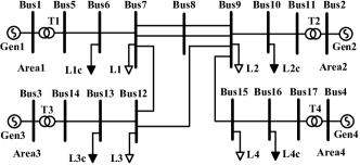
Figure 1: Four-area power system

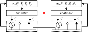
Figure 2: Closed-loop system diagram

TABLE I:
System parameters

Area $j$	$D_{j}$	$R_{j}$	$\alpha_{j}$	$\beta_{j}$	$T^{g}_{j}$	$T^{l}_{j}$
1	0.04	0.04	2	2.5	4	4
2	0.045	0.06	2.5	4	6	5
3	0.05	0.05	1.5	2.5	5	4
4	0.055	0.045	3	3	5.5	5

IV-B Simulation Results

In the simulation, the generations in each area are (625.9, 562.7, 701.7, 509.6) MW and the controllable loads are all 120 MW. The load changes are given in Table II, which are unknown to the controllers. Here we use the method mentioned in Remark 2 to estimate the load change. We also show the operational constraints on generations and controllable loads in individual control areas in Table II.

TABLE II:
Capacity limits and load disturbance

Area $j$	Load changes	[$\underline{P}^{g}_{j}$, $\overline{P}^{g}_{j}$] (MW)	[$\underline{P}^{l}_{j}$, $\overline{P}^{l}_{j}$] (MW)
1	90 MW	[600, 730]	[75, 120]
2	90 MW	[550, 680]	[80, 120]
3	90 MW	[650, 810]	[80, 120]
4	120 MW	[500, 640]	[55, 120]

IV-B1 Stability and optimality

The dynamics of local frequencies and tie-line power flows are illustrated in Fig.3. Both the frequency and tie-line power deviations are restored in all the four control areas. The generations and controllable loads are different from those before disturbance, indicating that the system is stabilized at a new equilibrium point. The resulting equilibrium point is given in Table III, which is identical to the optimal solution of (4) computed by centralized optimization using CVX. The simulation results confirm our theoretic analyses, verifying that our controller can autonomously guarantee the frequency stability while achieving optimal operating point in a completely decentralized manner.

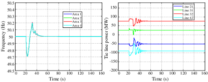
Figure 3: Dynamics of frequencies (left) and tie-line flows (right) in per-node balance case

TABLE III:
Equilibrium points

	Area 1	Area 2	Area 3	Area 4
$P^{g*}_{j}$ (MW)	676	618	758	570
$P^{l*}_{j}$ (MW)	80	85.3	86.2	60

IV-B2 Dynamic performance

In this subsection, we analyze the impacts of regulation capacity constraints on the dynamic performance. To this end, we compare the dynamic responses of the frequency controllers with and without input saturations. The trajectories of mechanical powers of turbines and controllable loads are shown in Fig.4 and Fig.5, respectively. In this case, the system frequency and tie-line flows are restored, and the same optimal equilibrium point is achieved. With the saturated controller, the mechanical power of turbines and controllable loads are strictly within the limits in transient. On the contrary, the controller without saturation results in considerable violation of the capacity constraints during transient, which is practically infeasible.

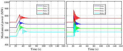
Figure 4: Mechanical outputs with(left)/without(right) capacity constraints

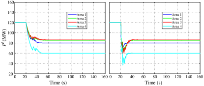
Figure 5: Controllable loads with(left)/without(right) capacity constraints

V Conclusion

We have proposed a decentralized optimal frequency control with aggregate generators and controllable loads. The controller can autonomously restore the nominal frequencies and tie-line powers after unknown load disturbances while minimizing the regulation cost. The capacity constraints on the generations and the controllable loads can always be satisfied even during transient. We have revealed that the closed-loop system carry out a primal-dual algorithm to solve the associated optimal dispatch problem, guaranteeing the optimality of closed-loop equilibria. We have used the projection technique combined with LaSalle’s invariance principle to prove the asymptotically stability of the closed-loop system. Simulations on the modified Kundur’s power system verify the efficacy of our designs.

Appendix A Proofs of Theorem 1 and Theorem 2

We start with a lemma.

Lemma A.1.

Suppose $(x^{*},u^{*})$ is optimal for (4). Then $\omega^{*}=0$ and $\theta^{*}=\theta^{*}_{0}\,\textbf{1}$ where 1 is the vector with all entries being 1.

Proof.

Suppose for the sake of contradiction that $\omega^{*}\neq 0$. Construct from $x^{*}$ another point $\hat{x}$ by setting $\hat{\theta}=0$, $\hat{\omega}=0$ and keeping the other components of $x^{*}$ unchanged. Since $x^{*}$ satisfies both (3) and (4d) we must have $U(\theta^{*},\omega^{*})=0$. This also holds for $\hat{x}$, i.e., $U(\hat{\theta},\hat{\omega})=0$, and hence $(\hat{x},u^{*})$ remains feasible since other components of $\hat{x}$ are the same as those of $x^{*}$. Moreover $(\hat{x},u^{*})$ has a strictly lower cost than $(x^{*},u^{*})$, contradicting the optimality of $(x^{*},u^{*})$. Hence any optimal $(x^{*},u^{*})$ must have $\omega^{*}=0$.

We claim that $\omega^{*}=0$ implies that $\theta^{*}=\theta^{*}_{0}\,\textbf{1}$. For any feasible point $x$, (3) and (4d) imply that

$$U(\theta,\omega) = D\omega+CBC^{T}\theta\ \ =\ \ 0$$

Hence we have $CBC^{T}\theta^{*}=0$ at an optimal $x^{*}$. Since $CBC^{T}$ is an $(n+1)\times(n+1)$ matrix with rank $n$, its null space has dimension 1. The vector 1 is in its null space because $C^{T}\textbf{1}=0$. Hence $\theta^{*}=\theta^{*}_{0}\,\textbf{1}$. ∎

Lemma A.1 at optimality implies that the frequencies are restored. Noticing that $\theta^{*}=\theta^{*}_{0}\,\textbf{1}$ means all angles are equal, such an optimal solution also implies that all the tie-line power flows are restored to their nominal values.

Lemma A.2.

Suppose $(x^{*},\rho^{*})$ is primal-dual optimal. Then

$$u^{g*}_{j}\ =\ P^{g*}_{j} = \left[P^{g*}_{j}-\gamma^{g}_{j}\left(\alpha_{j}P^{g*}_{j}+\omega^{*}_{j}+\lambda_{j}^{*}\right)\right]_{\underline{P}^{g}_{j}}^{\overline{P}^{g}_{j}}$$

$$u^{l*}_{j}\ =\ P^{l*}_{j} = \left[P^{l*}_{j}-\gamma^{l}_{j}\left(\beta_{j}P^{l*}_{j}-\omega^{*}_{j}-\lambda_{j}^{*}\right)\right]_{\underline{P}^{l}_{j}}^{\overline{P}^{l}_{j}}$$

for any $\gamma^{g}_{j}>0$ and $\gamma^{l}_{j}>0$.

Proof.

Since (4) is convex with linear constraints, strong duality holds. Hence $(x^{*},\rho^{*})$ is a primal-dual optimal if and only if it satisfies the KKT condition: $(x^{*},u(x^{*},\rho^{*}))$ is primal feasible and

$$x^{*} =\,\arg\min_{x}\left\{L_{1}(x;\rho^{*})|\,(x,u(x,\rho^{*}))\text{ satisfies }\eqref{eq:OpConstraints.1}\eqref{eq:opt.1b}\eqref{eq:opt.1c}\right\}$$ (A.1)

From the definition (10) of $L_{1}$, $x^{*}$ satisfies (A.1) if and only if $(x^{*},u(x^{*},\rho^{*}))$ satisfies (II) (4d) (4d) and the first-order stationarity condition, i.e., for all $j\in N$,

$$\!\!\!\!\alpha_{j}P^{g*}_{j}+\mu^{*}_{j}+\lambda^{*}_{j} \left\{\begin{array}[]{lll}\geq&0&\text{ if }P^{g*}_{j}=\underline{P}^{g}_{j}\\ =&0&\text{ if }\underline{P}^{g}_{j}<P^{g*}_{j}<\overline{P}^{g}_{j}\\ \leq&0&\text{ if }P^{g*}_{j}=\overline{P}^{g}_{j}\\ \end{array}\right.$$ (A.2d)

$$\!\!\!\!\beta_{j}P^{l*}_{j}-\mu^{*}_{j}-\lambda^{*}_{j} \left\{\begin{array}[]{lll}\geq&0&\text{ if }P^{l*}_{j}=\underline{P}^{l}_{j}\\ =&0&\text{ if }\underline{P}^{l}_{j}<P^{l*}_{j}<\overline{P}^{l}_{j}\\ \leq&0&\text{ if }P^{l*}_{j}=\overline{P}^{l}_{j}\\ \end{array}\right.$$ (A.2h)

$$D_{j}(\omega_{j}^{*}-\mu_{j}^{*}) \ \ \ \,=\ \ \,0$$ (A.2i)

$$\sum_{i:i\rightarrow j}B_{ij}(\mu^{*}_{i}-\mu^{*}_{j}) \ \ \ \,=\ \sum_{k:j\rightarrow k}B_{jk}(\mu^{*}_{j}-\mu^{*}_{k})$$ (A.2j)

From Lemma A.1 we have $$\omega^{*}=0 \mu^{*}=\omega^{*}=0 D_{j}>0$$ and hence (A.2) reduces to since and

$$\!\!\!\!\alpha_{j}P^{g*}_{j}+\omega^{*}_{j}+\lambda^{*}_{j} \left\{\begin{array}[]{lll}\geq&0&\text{ if }P^{g*}_{j}=\underline{P}^{g}_{j}\\ =&0&\text{ if }\underline{P}^{g}_{j}<P^{g*}_{j}<\overline{P}^{g}_{j}\\ \leq&0&\text{ if }P^{g*}_{j}=\overline{P}^{g}_{j}\\ \end{array}\right.$$ (A.3d)

$$\!\!\!\!\beta_{j}P^{l*}_{j}-\omega^{*}_{j}-\lambda^{*}_{j} \left\{\begin{array}[]{lll}\geq&0&\text{ if }P^{l*}_{j}=\underline{P}^{l}_{j}\\ =&0&\text{ if }\underline{P}^{l}_{j}<P^{l*}_{j}<\overline{P}^{l}_{j}\\ \leq&0&\text{ if }P^{l*}_{j}=\overline{P}^{l}_{j}\\ \end{array}\right.$$ (A.3h)

It can be checked that (A.3) is equivalent to

$$P^{g*}_{j} = \left[P^{g*}_{j}-\gamma^{g}_{j}\left(\alpha_{j}P^{g*}_{j}+\omega^{*}_{j}+\lambda_{j}^{*}\right)\right]_{\underline{P}^{g}_{j}}^{\overline{P}^{g}_{j}}$$

$$P^{l*}_{j} = \left[P^{l*}_{j}-\gamma^{l}_{j}\left(\beta_{j}P^{l*}_{j}-\omega^{*}_{j}-\lambda_{j}^{*}\right)\right]_{\underline{P}^{l}_{j}}^{\overline{P}^{l}_{j}}$$

for any $\gamma^{g}_{j}>0$ and $\gamma^{l}_{j}>0$. The lemma then follows from (4d)(4d). ∎

We now prove Theorems 1 and 2.

Proof of Theorem 1.

$\Rightarrow$: Suppose $(x^{*},\rho^{*})$ is primal-dual optimal. Then $x^{*}$ satisfies the operational constraints (II). Moreover the right-hand side of (2) vanishes because:

• $\dot{\theta}=0$ since $\omega^{*}=0$ from Lemma A.1.

• $\dot{\omega}=0$ because of (4d).

• $\dot{P}^{g}=\dot{P}^{l}=0$ since $\omega^{*}=0$ and $x^{*}$ satisfies (4d) and (4d).

The right-hand side of (6a) vanishes because $x^{*}$ satisfies per-node power balance (3). By Lemma A.2 $(x^{*},\rho^{*})$ satisfies (6b)(6c). Hence $(x^{*},\rho^{*})$ is an equilibrium of the closed-loop system (2)(6) that satisfies the operational constraints (II). Moreover $\mu^{*}=\omega^{*}=0$ by (A.2i) since $D_{j}>0$ for all $j\in N$.

$\Leftarrow$: Suppose now $(x^{*},\rho^{*})$ is an equilibrium of the closed-loop system (2)(6) and satisfies (II) with $\mu^{*}=0$. Since (4) is convex with linear constraints, $(x^{*},\rho^{*})$ is a primal-dual optimal if and only if $(x^{*},u(x^{*},\rho^{*}))$ is primal feasible and satisfies (A.1) (note that $\nabla_{\rho}L_{1}(x^{*},\rho^{*})=0$ since $\dot{\mu}=\dot{\lambda}=0$).

To show that $(x^{*},u(x^{*},\rho^{*}))$ is primal feasible, note that since $(x^{*},u(x^{*},\rho^{*}))$ is an equilibrium of (2), it satisfies $\omega^{*}=0$, (4d)(4d)(4d), in addition to (II). Since $(x^{*},\rho^{*})$ is a closed-loop equilibrium, we have $\dot{\lambda}^{*}\equiv 0$ in (6a), implying (3). Hence $x^{*}$ is primal feasible.

To show that $(x^{*},\rho^{*})$ satisfies (A.1), note that (4d)(4d) and (6b)(6c) imply that

$$P^{g*}_{j} = \left[P^{g*}_{j}-\gamma^{g}_{j}\left(\alpha_{j}P^{g*}_{j}+\omega^{*}_{j}+\lambda_{j}^{*}\right)\right]_{\underline{P}^{g}_{j}}^{\overline{P}^{g}_{j}}$$

$$P^{l*}_{j} = \left[P^{l*}_{j}-\gamma^{l}_{j}\left(\beta_{j}P^{l*}_{j}-\omega^{*}_{j}-\lambda_{j}^{*}\right)\right]_{\underline{P}^{l}_{j}}^{\overline{P}^{l}_{j}}$$

for any $\gamma^{g}_{j}>0$ and $\gamma^{l}_{j}>0$. This is equivalent to (A.3). Since $\mu^{*}=\omega^{*}=0$, (A.3) is equivalent to (A.2) which is equivalent to (A.1). This proves that $(x^{*},\rho^{*})$ is primal-dual optimal and completes the proof of Theorem 1. ∎

Next we prove Theorem 2.

Proof of Theorem 2.

Let $(x^{*},\rho^{*})=(\theta^{*},\omega^{*},P^{g*},P^{l*},$ $\lambda^{*},\mu^{*})$ be primal-dual optimal. Lemma A.1 implies that $\omega^{*}=0$ and $\theta^{*}$ is unique up to the reference angle $\theta_{0}^{*}$. This proves parts 3 and 4 of Theorem 2.

To prove part 1 of the theorem, since the objective function is strictly convex in $\left(P^{g},P^{l}\right)$ the optimal values $\left(P^{g*},P^{l*}\right)$ are unique. Hence $x^{*}$ is unique (up to $\theta_{0}^{*}$).

As for the part 2 of the theorem, from (A.2i) in the proof of Lemma A.2, we have $\mu^{*}=\omega^{*}=0$, implying the uniqueness of $\mu^{*}$. From (A.2d)(A.2h), $\lambda_{j}^{*}$ is unique if either $\underline{P}^{g}_{j}<P^{g*}_{j}<\overline{P}^{g}_{j}$ or $\underline{P}^{l}_{j}<P^{l*}_{j}<\overline{P}^{l}_{j}$. We now prove that this is indeed the case by showing that the other four cases cannot hold: (i) $P^{g*}_{j}=\underline{P}^{g}_{j}$ and $P^{l*}_{j}=\underline{P}^{l}_{j}$; (ii) $P^{g*}_{j}=\underline{P}^{g}_{j}$ and $P^{l*}_{j}=\overline{P}^{l}_{j}$; (iii) $P^{g*}_{j}=\overline{P}^{g}_{j}$ and $P^{l*}_{j}=\underline{P}^{l}_{j}$; and (iv) $P^{g*}_{j}=\overline{P}^{g}_{j}$ and $P^{l*}_{j}=\overline{P}^{l}_{j}$.

Since $P^{g*}_{j}-P^{l*}_{j}=p_{j}$ for per-node power balance, (ii) and (iii) cannot hold since the inequalities in A2 are strict. Suppose (i) holds. Then there exists an $\epsilon_{j}>0$ such that $\hat{P}^{g}_{j}=\underline{P}^{g}_{j}+\epsilon_{j}<0$ and $\hat{P}^{l}_{j}=\underline{P}^{l}_{j}+\epsilon_{j}<0$, together with other components of $x^{*}$, remain a feasible primal solution. However this new feasible solution attains a strictly smaller objective value, contradicting the optimality of $x^{*}$. Thus (i) cannot hold. Similarly (iv) cannot hold. This proves that $\lambda^{*}$ is unique.

Finally, if $\underline{P}^{g}_{j}<P^{g*}_{j}<\overline{P}^{g}_{j}$ then $\lambda^{*}_{j}$ is uniquely determined by $\lambda^{*}_{j}=-\alpha_{j}P^{g*}_{j}$ according to (A.2d). If $\underline{P}^{l}_{j}<P^{l*}_{j}<\overline{P}^{l}_{j}$ then $\lambda^{*}_{j}$ is uniquely determined by $\lambda^{*}_{j}=\beta P^{l*}_{j}$ according to (A.2h).

This completes the proof of Theorem 2.

∎

Appendix B Proofs of Lemma 3 and Theorem 4

We prove Lemma 3 using the first-order inertia dynamics of (6b) and (6c).

Proof of Lemma 3. Set

$$\hat{u}_{j}^{g}(t) = \left[P^{g}_{j}(t)-\gamma^{g}_{j}\left(\alpha_{j}P^{g}_{j}(t)+\omega_{j}(t)+\lambda_{j}(t)\right)\right]_{\underline{P}^{g}_{j}}^{\overline{P}^{g}_{j}}$$

Then (1c) can be rewritten as

$$T_{j}^{g}\dot{P}_{j}^{g}(t)+P_{j}^{g}(t)=\hat{u}_{j}^{g}(t)$$ (B.1)

Apply the Laplace transform to (B.1) to obtain

$${\cal L}\left(P_{j}^{g}\right)(s)={\cal L}\left(\hat{u}_{j}^{g}\right)(s)/(T_{j}^{g}s+1).$$

In the time domain $P_{j}^{g}(t)$ is then given by convolution:

$$P_{j}^{g}\left(t\right) =\ \frac{1}{{{T_{j}^{g}}}}\int_{{0^{-}}}^{+\infty}{\hat{u}_{j}^{g}\left({t-\tau}\right){e^{-\tau/{T_{j}^{g}}}}d\tau}$$

$$=\ \int_{0}^{\frac{t}{T^{g}_{j}}}\hat{u}_{j}^{g}\left(t-T^{g}_{j}\tau\right){e^{-\tau}}d\tau$$

Since $e^{-\tau}>0$ we can replace $\hat{u}_{j}^{g}$ in the integrand by its lower and upper bounds $\underline{P}^{g}_{j}$ and $\overline{P}^{g}_{j}$ respectively to conclude

$$\int_{0}^{\frac{t}{T^{g}_{j}}}\underline{P}^{g}_{j}\cdot e^{-\tau}d\tau \leq\ \ P_{j}^{g}\left(t\right)\ \ \leq \int_{0}^{\frac{t}{T^{g}_{j}}}\overline{P}^{g}_{j}\cdot e^{-\tau}d\tau$$

Hence

$$\underline{P}_{j}^{g}\left({1-{e^{-t/{T_{j}^{g}}}}}\right)\ \ \leq\ \ P_{j}^{g}\left(t\right)\ \ \leq\ \ \overline{P}_{j}^{g}\left({1-{e^{-t/{T_{j}^{g}}}}}\right)$$

and $P_{j}^{g}\leq P_{j}^{g}\left(t\right)\leq\overline{P}_{j}^{g}$ for all $t\geq 0$ under assumptions A1 and A3. That $\underline{P}_{j}^{l}\leq P_{j}^{l}\left(t\right)\leq\overline{P}_{j}^{l}$ can be proved similarly. ∎

Proof of Theorem 4. We start with a lemma.

Lemma B.1.

Suppose A1, A2 and A3 hold. Given any $w(0)\in S$ we have

1. $\dot{V}_{1}(w(t))\leq 0,\forall t>0$.

2. The trajectory $w(t)$ is bounded, i.e., there exists $\overline{w}$ such that $\|w(t)\|\leq\overline{w}$ for all $t\geq 0$.

Proof of Lemma B.1 We omit $t$ in the proof for simplicity. According [27, Theorem 3.2], since $F(w)$ is continuously differentiable, $V_{1}(w)$ defined by (III-E) is also continuously differentiable. Moreover its gradient is given by

$$\nabla_{w}V_{1}(w) \!\!\!\!\!\!= \!\!\!\!\!\!F(w)-(\nabla_{w}F(w)-I)(H(w)-w)+k\Gamma_{1}^{-2}(w-w^{*})$$

Then the derivative of $V_{1}(w)$ along the solution trajectory is

$$\dot{V}_{1}(w) =\nabla_{w}^{T}V_{1}(w)\cdot\dot{w}\ \ =\ \ \nabla_{w}^{T}V_{1}(w)\cdot\Gamma_{1}(H(w)-w)$$

$$=(F(w)-\left(\nabla_{w}F(w)-I)(H(w)-w))^{T}\Gamma_{1}(H(w)-w\right)$$

$$\quad+k(w-w^{*})\cdot\Gamma_{1}^{-1}(H(w)-w)$$

$$=-(H(w)-w)^{T}\nabla_{w}F(w)\Gamma_{1}(H(w)-w)$$

$$\quad-\left(H(w)-(w-F(w))\right)^{T}\Gamma_{1}(w-H(w))$$

$$\quad+k(w-w^{*})^{T}\cdot\Gamma_{1}^{-1}(H(w)-F(w)+F(w)-w)$$

$$=-(H(w)-w)^{T}\nabla_{w}F(w)\Gamma_{1}(H(w)-w)$$

$$\quad-\left(H(w)-(w-F(w))\right)^{T}\Gamma_{1}(w-H(w))$$

$$\quad-k(w-w^{*})^{T}\cdot\Gamma_{1}^{-1}F(w)$$

$$\quad+k(w-H(w)+H(w)-w^{*})^{T}\Gamma_{1}^{-1}(H(w)-(w-F(w)))$$

$$=k(H(w)-w^{*})^{T}\cdot\Gamma_{1}^{-1}(H(w)-(w-F(w)))$$ (B.2a)

$$\quad-\left(H(w)-(w-F(w))\right)^{T}(\Gamma_{1}-k\Gamma_{1}^{-1})(w-H(w))$$ (B.2b)

$$\quad-(H(w)-w)^{T}\nabla_{w}F(w)\cdot\Gamma_{1}(H(w)-w)$$ (B.2c)

$$\quad-k(w-w^{*})^{T}\cdot\Gamma_{1}^{-1}F(w)$$ (B.2d)

where $$\Gamma_{1}:=\text{diag}\left(B^{-1/2},M^{-1/2},(T^{g})^{-1},(T^{l})^{-1},(\Gamma_{1}^{\lambda})^{1/2}\right) \dot{V}_{1}(w)\leq 0$$ is diagonal and positive definite. We now prove that all terms on the right-hand side are nonpositive and hence .

$$\nabla_{w}F(w) := \underbrace{\begin{bmatrix}B^{-1/2}&0&0&0&0\\ 0&M^{-1/2}&0&0&0\\ 0&0&(T^{g})^{-1}&0&0\\ 0&0&0&(T^{l})^{-1}&0\\ 0&0&0&0&(\Gamma^{\lambda})^{1/2}\end{bmatrix}}_{\Gamma_{1}}\cdot\left[\begin{array}[]{c c c c c}0&-BC^{T}&0&0&0\\ CB&D&-I&I&0\\ 0&I&A^{g}&0&I\\ 0&-I&0&A^{l}&-I\\ 0&0&-I&I&0\\ \end{array}\right]$$ (B.12)

For the term in (B.2a) denote the projection of any $w$ onto $S$ under the norm defined by a (symmetric) positive definite matrix $\Gamma$ by

$$\text{Proj}_{S,\Gamma}(w) := \arg\min_{y\in S}\ (y-w)^{T}\Gamma(y-w)$$

By the projection theorem a vector $\hat{w}_{\Gamma}$ is equal to the projection $\text{Proj}_{S,\Gamma}(w)$ if and only if

$$\left(\hat{w}_{\Gamma}-w\right)^{T}\Gamma\left(y-\hat{w}_{\Gamma}\right) \geq 0,\qquad y\in S$$ (B.3)

Note that $S=:\prod_{i}S_{i}$ is a direct product of intervals $S_{i}$ and $\Gamma=\text{diag}(\Gamma_{ii})$ is diagonal. Hence the projection under the $\Gamma$-norm coincide with the projection under the Euclidean norm:

$$\text{Proj}_{S,\Gamma}(w) = \arg\min_{y:y_{i}\in S_{i}}\ \sum_{i}\,\Gamma_{ii}(y_{i}-w_{i})^{2}$$

$$= \arg\min_{y:y_{i}\in S_{i}}\ \sum_{i}\,(y_{i}-w_{i})^{2}\ \ =\ \ \text{Proj}_{S}(w)$$

Substituting into (B.3) we have, for any diagonal positive definite $\Gamma$,

$$\left(\text{Proj}_{S}(w)-w\right)^{T}\Gamma\left(y-\text{Proj}_{S}(w)\right) \geq 0,\quad y\in S$$ (B.4)

for any $w$. The projection $H(w):=\text{Proj}_{S}(w-F(w))$ of $w-F(w)$ therefore satisfies (for $\Gamma:=\Gamma_{1}^{-1}$)

$$\left(H(w)-(w-F(w)\right)^{T}\Gamma_{1}^{-1}\left(w^{*}-H(w)\right) \geq 0$$ (B.5)

since $w^{*}\in S$. This proves that the right-hand side of (B.2a) is nonpositive

To show that (B.2b) is nonpositive we use a similar argument. Since $\Gamma:=\Gamma_{1}-k\Gamma_{1}^{-1}>0$ we can define the projection $\text{Proj}_{S,\Gamma}(w)$ under this $\Gamma$. As explained above $\text{Proj}_{S,\Gamma}(w)=\text{Proj}_{S}(w)$ and hence as before, we have

$$\left(H(w)-(w-F(w)\right)^{T}\Gamma\left(w-H(w)\right) \geq 0$$

since the solution trajectory $w(t)\in S$ for all $t\geq 0$ by Lemma 3. This proves the term in (B.2b) is nonpositive.

We will prove that (B.2d) is nonpositive. Along any solution trajectory we always have $\mu(t)\equiv\omega(t)$. Substituting into the Lagrangian $L_{1}(x,\rho)$ in (10) we obtain a function

$$\hat{L}_{1}(\tilde{\theta},P^{g},P^{l},\lambda,\omega)\ \ :=\ \ L_{1}(\theta,\omega,P^{g},P^{l},\lambda,\omega)$$

$$= \frac{1}{2}\left((P^{g})^{T}A^{g}P^{g}+(P^{l})^{T}A^{l}P^{l}-\omega^{T}D\omega\right)$$

$$+\ \lambda^{T}\!\!\left(P^{g}-P^{l}-p\right)+\ \omega^{T}\!\!\left(P^{g}-P^{l}-p-CB\tilde{\theta}\right)$$

Write $w_{1}:=(\tilde{\theta},P^{g},P^{l})$, $w_{2}:=(\lambda,\omega)$. Then $\hat{L}_{1}(w_{1},w_{2})$ is convex in $w_{1}$ and concave in $w_{2}$. It can be verified that

$$\Gamma_{1}^{-1}F(w) \!\!\!\!=\!\!\!\! \begin{bmatrix}\nabla_{\tilde{\theta}}\hat{L}_{1}\\ \nabla_{P^{g}}\hat{L}_{1}\\ \nabla_{P^{l}}\hat{L}_{1}\\ -\nabla_{\lambda}\hat{L}_{1}\\ -\nabla_{\omega}\hat{L}_{1}\end{bmatrix}(w_{1},w_{2})\ =\ \begin{bmatrix}\ \ \nabla_{w_{1}}\hat{L}_{1}\\ -\nabla_{w_{2}}\hat{L}_{1}\end{bmatrix}\!(w_{1},w_{2})$$

Hence, we have

$$\ -k(w-w^{*})^{T}\cdot\Gamma_{1}^{-1}F(w)$$

$$= \ -k(w_{1}-w_{1}^{*})^{T}\nabla_{w_{1}}\hat{L}_{1}(w_{1},w_{2})+k(w_{2}-w_{2}^{*})^{T}\nabla_{w_{2}}\hat{L}_{1}(w_{1},w_{2})$$

$$\leq \ k\bigg{(}\hat{L}_{1}(w_{1}^{*},w_{2})-\hat{L}_{1}(w_{1},w_{2})+\hat{L}_{1}(w_{1},w_{2})-\hat{L}_{1}(w_{1},w^{*}_{2})\bigg{)}$$

$$= \ k\bigg{(}\hat{L}_{1}(w_{1}^{*},w_{2})-\hat{L}_{1}(w^{*}_{1},w^{*}_{2})+\hat{L}_{1}(w^{*}_{1},w^{*}_{2})-\hat{L}_{1}(w_{1},w^{*}_{2})\bigg{)}$$

$$\leq \ 0$$ (B.6)

where the first inequality follows because $\hat{L}_{1}$ is convex in $w_{1}$ and concave in $w_{2}$ and the second inequality follows because $(w^{*}_{1},w^{*}_{2})$ is a saddle point. Therefore (B.2d) is nonpositive.

Finally to prove that (B.2c) is nonpositive note that

$$(H(w)-w)^{T}\nabla_{w}F(w)\Gamma_{1}(H(w)-w) \!\!\!\!=\!\!\!\! \dot{w}^{T}\left(\Gamma_{1}^{-1}\nabla_{w}F(w)\right)\dot{w}$$

where $\dot{w}:=(\dot{\tilde{\theta}},\dot{\omega},\dot{P}^{g},\dot{P}^{l},\dot{\lambda})$. From (20), $\nabla_{w}F(w)$ is given by (B.12).

Hence

$$\dot{w}^{T}\left(\Gamma_{1}^{-1}\nabla_{w}F(w)\right)\dot{w} \!\!\!\!=\!\!\!\! \dot{\omega}^{T}D\dot{\omega}\,+\,\dot{P}^{gT}A^{g}\dot{P}^{g}\,+\,\dot{P}^{lT}A^{l}\dot{P}^{l}\,\geq\,0$$

and hence (B.2c) is nonpositive.

This also implies that

$$\dot{V}_{1}(w(t)) \leq-\left(\dot{\omega}^{T}D\dot{\omega}\,+\,\dot{P}^{gT}A^{g}\dot{P}^{g}\,+\,\dot{P}^{lT}A^{l}\dot{P}^{l}\right)\ \,\leq\ \,0$$ (B.8)

for all $t\geq 0$. This proves the first assertion of the lemma.

To prove that the trajectory $w(t)$ is bounded note that [27, Theorem 3.1] proves that $\hat{V}_{1}(w):=-\left(H(w)-w\right)^{T}F(w)\,-\,\frac{1}{2}||H(w)-w||^{2}_{2}$ satisfies $\hat{V}_{1}(w)\geq 0$ over $S$. Hence

$$\frac{1}{2}k(w(t)-w^{*})^{T}\Gamma_{1}^{-2}(w(t)-w^{*}) \!\!\!\leq\!\!\! V_{1}(w(t))\ \leq\ V_{1}(w(0))$$

indicating the trajectory $w(t)$ is bounded, as desired. ∎

Lemma B.2.

Suppose A1, A2 and A3 hold. Given any $w(0)\in S$, we have

1. The trajectory $w(t)$ converges to the largest invariant set $W_{1}^{*}$ contained in $W_{1}=\{w\in S|\ \dot{P}^{g}=\dot{P}^{l}=\dot{\omega}=0\}$.

2. Every point $w^{*}\in W_{1}^{*}$ is an equilibrium point of (21).

Proof of Lemma B.2.

Fix any initial state $w(0)$ and consider the trajectory $(w(t),t\geq 0)$ of the closed-loop system (21). Lemma B.1 implies a compact set $\Omega_{0}:=\Omega(w(0))\subset S$ such that $w(t)\in\Omega_{0}$ for $t\geq 0$ and $\dot{V}_{1}(w)\leq 0$ in $\Omega_{0}$. Let $W_{1}:=\{w\in\Omega_{0}|\ \dot{P}^{g}=\dot{P}^{l}=\dot{\omega}=0\}$. Then (B.8) implies that $w\in W_{1}$ if and only if $\dot{V}_{1}(w)=0$. According to LaSalle’s invariance principle ([31, Theorem 4.4]) the solution trajectory $(w(t),t\geq 0)$ converges to the largest invariant set contained in $W_{1}$, proving the first assertion.

For the second assertion, fix any $w(0)\in W_{1}^{*}$. We claim that $w(0)$ must be an equilibrium point of (21). Since $W_{1}^{*}$ is invariant we have

$$\dot{P}^{g}(t)\ =\ \dot{P}^{l}(t)\ =\ \dot{\omega}(t)\ =\ 0,\quad t\geq 0$$ (B.9)

It suffices to prove that $\dot{w}(t)=0$ for $t\geq 0$, i.e., $\dot{\tilde{\theta}}=0$ and $\dot{\lambda}=0$ for $t\geq 0$.

Since $P^{g}(t),P^{l}(t),\omega(t)$ are bounded (Lemma B.1), (B.9) implies that

$$(P^{g}(t),P^{l}(t),\omega(t))\ \equiv\ (P^{g\infty},P^{l\infty},\omega^{\infty})$$

for some finite constants $(P^{g\infty},P^{l\infty},\omega^{\infty})$. Hence

$$\dot{\tilde{\theta}}(t) = C^{T}\omega^{\infty}\ \ =\ \ \text{constant}$$

implying that $\tilde{\theta}(t)$ grows linearly in $t$, contradicting that $\tilde{\theta}(t)$ is bounded unless $\dot{\tilde{\theta}}=0$ for $t\geq 0$. Similarly

$$\dot{\lambda}(t) = \Gamma^{\lambda}\left(P^{g\infty}-P^{l\infty}-p\right)\ \ =\ \ \text{constant}$$

Hence the boundedness of $\lambda(t)$ implies that $\dot{\lambda}(t)=0$ for $t\geq 0$. This proves that any $w(0)\in W_{1}^{*}$ is an equilibrium point. ∎

If all inequalities in A2 are strict, then the equilibrium point $w^{*}$ of the closed-loop system (21) is unique (Theorem 2.2) and Lemma B.2 implies that $w(t)$ converges to $w^{*}$ [31, Corollary 4.1, p. 128] as $t\to\infty$. When there are multiple equilibrium points, Lemma B.2 is not adequate to conclude asymptotic stability. We use instead a more direct argument due to [12, 6].

Proof of Theorem 4.

Fix any initial state $w(0)$ and consider the trajectory $(w(t),t\geq 0)$ of the closed-loop system (21). As mentioned in the proof of Lemma B.2, $w(t)$ stays entirely in a compact set $\Omega_{0}$. Hence there exists an infinite sequence of time instants ${t_{k}}$ such that $w(t_{k})\to\hat{w}^{*}$ as $k\to\infty$, for some $\hat{w}^{*}$ in $W_{1}^{*}$. Lemma B.2 guarantees that $\hat{w}^{*}$ is an equilibrium point of the closed-loop system (21) and hence $H(\hat{w}^{*})=\hat{w}^{*}$. Use this specific equilibrium point $\hat{w}^{*}$ in the definition of $V_{1}$ in (III-E) to get the Lyapunov function:

$$V_{1}(w) =-\left(H(w)-w\right)^{T}F(w)\,-\,\frac{1}{2}||H(w)-w||^{2}_{2}$$

$$\quad+\frac{1}{2}k(w-\hat{w}^{*})^{T}\Gamma_{1}^{-2}(w-\hat{w}^{*})$$

Since $\dot{V}_{1}\leq 0$, $V_{1}(w(t))$ converges. Moreover it follows from the continuity of $V_{1}$ that

$$\lim_{t\to\infty}V_{1}(w(t))\ \ =\ \ \lim_{k\to\infty}V_{1}(w(t_{k})) = V_{1}(\hat{w}^{*})\ \ =\ \ 0$$

The quadratic term $(w-\hat{w}^{*})^{T}\Gamma_{1}^{-2}(w-\hat{w}^{*})$ in $V_{1}$ then implies that $w(t)\to\hat{w}^{*}$ as $t\to\infty$. ∎

References

- [1] L. Min and A. Abur, “Total transfer capability computation for multi-area power systems,” IEEE Trans. Power Syst., vol. 21, no. 3, pp. 1141–1147, Aug. 2006.
- [2] A. Ahmadi-Khatir, M. Bozorg, and R. Cherkaoui, “Probabilistic spinning reserve provision model in multi-control zone power system,” IEEE Trans. Power Syst., vol. 28, no. 3, pp. 2819–2829, Mar. 2013.
- [3] I. Ibraheem, P. Kumar, and D. P. Kothari, “Recent philosophies of automatic generation control strategies in power systems,” IEEE Trans. Power Syst., vol. 20, no. 1, pp. 346–357, Feb. 2005.
- [4] M. H. Variani and K. Tomsovic, “Distributed automatic generation control using flatness-based approach for high penetration of wind generation,” IEEE Trans. Power Syst., vol. 28, no. 3, pp. 3002–3009, Apr. 2013.
- [5] T. Stegink, C. D. Persis, and A. van der Schaft, “A unifying energy-based approach to stability of power grids with market dynamics,” arXiv preprint arXiv:1604.05200, 2016.
- [6] N. Li, C. Zhao, and L. Chen, “Connecting automatic generation control and economic dispatch from an optimization view,” IEEE Trans. Control Netw. Syst., vol. 3, no. 3, pp. 254–264, September 2016.
- [7] T. Stegink, C. D. Persis, and A. van der Schaft, “A port-hamiltonian approach to optimal frequency regulation in power grids,” in Proc. 54th IEEE Conference on Decision and Control (CDC), Dec 2015, pp. 3224–3229.
- [8] Z. Wang, F. Liu, L. Chen, and S. Mei, “Distributed economic automatic generation control: A game theoretic perspective,” in Power Energy Society General Meeting, 2015 IEEE, Denver, CO, July 2015, pp. 1–5.
- [9] Z. Wang, F. Liu, S. H. Low, C. Zhao, and S. Mei, “Decentralized optimal frequency control of interconnected power systems with transient constraints,” in 2016 IEEE 55th Conference on Decision and Control (CDC), Dec 2016, pp. 664–671.
- [10] M. D. Ilic, L. Xie, U. A. Khan, and J. M. F. Moura, “Modeling of future cyber-physical energy systems for distributed sensing and control,” IEEE Trans. Systems, Man, Cybern. A, Syst. Hum, vol. 40, no. 4, pp. 825–838, July 2010.
- [11] M. Zribi, M. Al-Rashed, and M. Alrifai, “Adaptive decentralized load frequency control of multi-area power systems,” Int. J. Elect. Power Energy Syst., vol. 27, no. 8, pp. 575–583, Oct. 2013.
- [12] C. Zhao, U. Topcu, N. Li, and S. H.Low., “Design and stability of load-side primary frequency control in power systems,” IEEE Trans. Autom. Control, vol. 59, no. 5, pp. 1177–1189, Jan. 2014.
- [13] C. Zhao and S. H. Low, “Decentralized primary frequency control in power networks,” in Proc. 53th IEEE Conference on Decision and Control (CDC), December 2014, pp. 2467–2473.
- [14] E. Mallada, C. Zhao, and S. H. Low, “Optimal load-side control for frequency regulation in smart grids,” IEEE Trans. Autom. Control, to appear, 2017.
- [15] A. Kasis, E. Devane, C. Spanias, and I. Lestas, “Primary frequency regulation with load-side participation part i: stability and optimality,” IEEE Trans. Power Syst. early access, 2016.
- [16] E. Devane, A. Kasis, M. Antoniou, and I. Lestas, “Primary frequency regulation with load-side participation part ii: beyond passivity approaches,” IEEE Trans. Power Syst. early access, 2016.
- [17] A. Maknouninejad, Z. Qu, F. L. Lewis, and A. Davoudi, “Optimal, nonlinear, and distributed designs of droop controls for dc microgrids,” IEEE Trans. Smart Grid, vol. 5, no. 5, pp. 2508–2516, Sept 2014.
- [18] V. Nasirian, A. Davoudi, F. L. Lewis, and J. M. Guerrero, “Distributed adaptive droop control for dc distribution systems,” IEEE Trans. Energy Convers, vol. 29, no. 4, pp. 944–956, Dec 2014.
- [19] R. Olfati-Saber, J. A. Fax, and R. M. Murray, “Consensus and cooperation in networked multi-agent systems,” Proc. IEEE, vol. 95, no. 1, pp. 215–233, Jan 2007.
- [20] G. Binetti, A. Davoudi, F. L. Lewis, D. Naso, and B. Turchiano, “Distributed consensus-based economic dispatch with transmission losses,” IEEE Trans. Power Syst., vol. 29, no. 4, pp. 1711–1720, July 2014.
- [21] H. Xin, Z. Lu, Z. Qu, D. Gan, and D. Qi, “Cooperative control strategy for multiple photovoltaic generators in distribution networks,” IET Control Theory Applicat, vol. 5, no. 14, pp. 1617–1629, Sept 2011.
- [22] A. Jokić, M. Lazar, and P. P. van den Bosch, “Real-time control of power systems using nodal prices,” Int. J. Elect. Power Energy Syst., vol. 31, no. 9, pp. 522–530, 2009.
- [23] D. P. Bertsekas., Nonlinear programming, 2nd ed. Athena scientific, 2008.
- [24] K. J. Arrow, L. Hurwicz, H. Uzawa, and H. B. Chenery, Studies in linear and non-linear programming. Stanford University Press Stanford, 1958.
- [25] D. Feijer and F. Paganini, “Stability of primal–dual gradient dynamics and applications to network optimization,” Automatica, vol. 46, no. 12, pp. 1974–1981, 2010.
- [26] A. Rantzer, “Dynamic dual decomposition for distributed control,” in Proc. of American Control Conference (ACC), St. Louis, MO, USA, 2009, pp. 884–888.
- [27] M. Fukushima, “Equivalent differentiable optimization problems and descent methods for asymmetric variational inequality problems,” Math. programming, vol. 53, no. 1-3, pp. 99–110, Jan 1992.
- [28] J. Fang, W. Yao, Z. Chen, J. Wen, and S. Cheng, “Design of anti-windup compensator for energy storage-based damping controller to enhance power system stability,” IEEE Trans. Power Syst., vol. 29, no. 3, pp. 1175–1185, May 2014.
- [29] P. Kundur, Power System Stability and Control. McGraw-hill New York, 1994, vol. 7.
- [30] https://hvdc.ca/pscad/.
- [31] H. K. Khalil, Nonlinear systems. Prentice hall New Jersey, 1996, vol. 3.