Supervised Learning of Labeled Pointcloud Differences via Cover-Tree Entropy Reduction

Abstract.

We introduce a new algorithm, called CDER, for supervised machine learning that merges the multi-scale geometric properties of Cover Trees with the information-theoretic properties of entropy. CDER applies to a training set of labeled pointclouds embedded in a common Euclidean space. If typical pointclouds corresponding to distinct labels tend to differ at any scale in any sub-region, CDER can identify these differences in linear time, creating a set of distributional coordinates which act as a feature extraction mechanism for supervised learning. We describe theoretical properties and implementation details of CDER, and illustrate its benefits on several synthetic examples.

1. Overview and Assumptions

We propose a new supervised machine-learning method for classification, where each object to be classified is a weighted pointcloud, and the classification task is to learn which of a finite set of labels should be applied to the pointcloud. The method is fast, data-driven, multi-scale, and requires no tuning. Additionally, its details are transparently geometric; it does not suffer from the “black box” interpretation difficulties that arise in many machine-learning methods. We call it Cover-tree Differencing via Entropy Reduction [CDER, pronounced “cedar”].

A high-level sketch of CDER is as follows. We construct a partial cover tree [7] on the union of all labeled pointclouds that are given in some training set, and we search the cover tree for convex regions that are likely to be local minima of entropy [3]. For each such region, we build distributional coordinates from the dominant labels’ data. An ordered sequence of these distributional coordinates allows us to determine the likelihood of each label for an unlabeled test pointcloud.

Section 3 explains the notion of distributional coordinates defined on pointclouds as a front-end for supervised learning. Section 4 details the cover-tree algorithm and our enhancements to it. Section 5 explains our simple approach to entropy minimization in the labeled pointcloud context. Section 6 gives a formal description of CDER. Section 7 illustrates CDER with several synthetic examples. The remainder of this section establishes context and notation for this problem.

Fix a Euclidean space $\mathbb{R}^{D}$. A pointcloud is a finite set $X=\{x_{1},x_{2},\ldots,x_{|X|}\}\subset\mathbb{R}^{D}$. We allow weighted pointclouds, where each $x\in X$ has a positive weight $w(x)$; the utility of weights is explained in Section 2. A cloud collection is a finite set of pointclouds

$$\mathcal{X}=\{X_{1},X_{2},\ldots,X_{N}\},$$

with $N=|\mathcal{X}|$. Let $\underline{\mathcal{X}}=\bigcup_{i=1}^{N}X_{i}\subset M$ denote the union of all pointclouds in a cloud collection, which is itself a pointcloud with weights and labels of each point $x\in\underline{\mathcal{X}}$ inherited from the respective $X_{i}\owns x$.

For our supervised learning task, the training data is a cloud collection $\mathcal{X}$, where each pointcloud is labeled from a finite set of labels, $\Lambda$. For the sake of discussion and visualization, we usually interpret $\Lambda$ as a set of colors, but for mathematical purposes, $\Lambda=\{1,\ldots,L\}$ where $L=|\Lambda|$. Let $\lambda:\mathcal{X}\to\Lambda$ denote the label function, and we also use $\lambda$ to indicate a generic label in $\Lambda$.

It is acceptable that the pointclouds $X_{i}$ have unequal sizes across $X_{i}\in\mathcal{X}$. It is also acceptable that the labeled sub-collections $\mathcal{X}|_{\lambda}=\{X_{i}~{}:~{}\lambda(X_{i})=\lambda\}=\lambda^{-1}(\lambda)$ have unequal sizes across labels $\lambda\in\Lambda$. Pointwise weights can be assigned to compensate for these sizes, as in Section 2. Our only structural hypothesis is that, for each labeled sub-collection, the pointclouds are sampled from an underlying density function—or from several density functions as chosen by a random process—on $\mathbb{R}^{D}$. For each label $\lambda$, let $f_{\lambda}$ denote this density function.

We aim to efficiently find regions in $\mathbb{R}^{D}$ where one label has greater density than the other labels. That is, we seek convex regions $\Omega\subset\mathbb{R}^{D}$ that are “characteristic” of a particular label $\lambda$ because $f_{\lambda}$ is unusually prominent there, while ignoring regions where the various density functions are similar. See Figure 1.

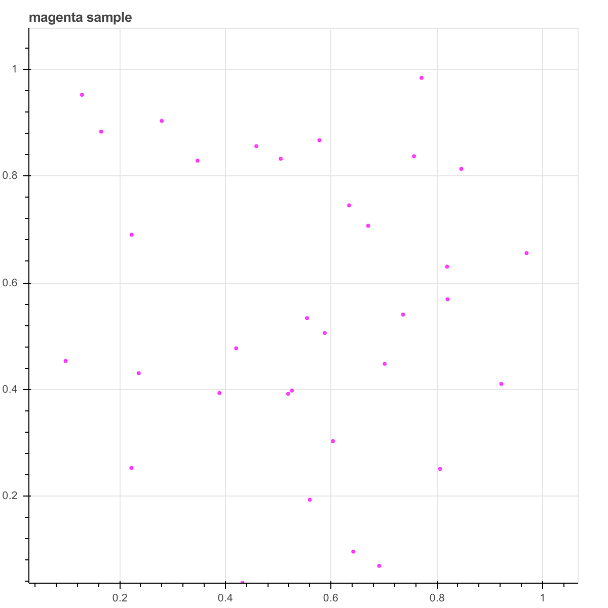
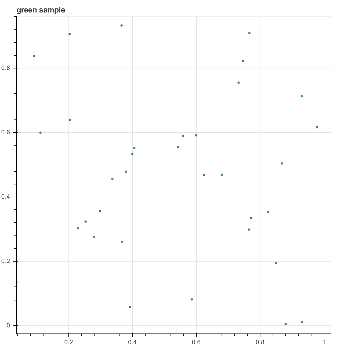
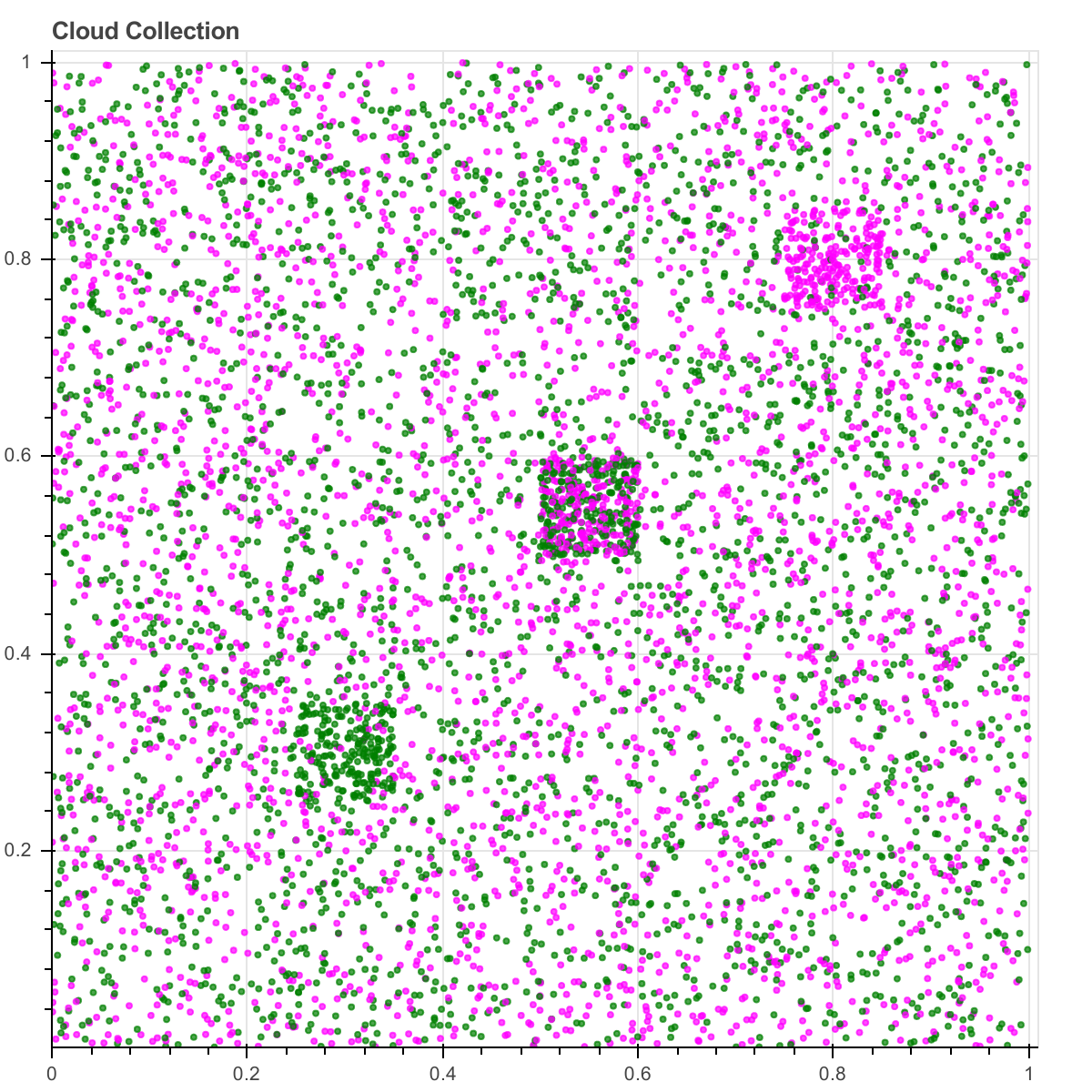
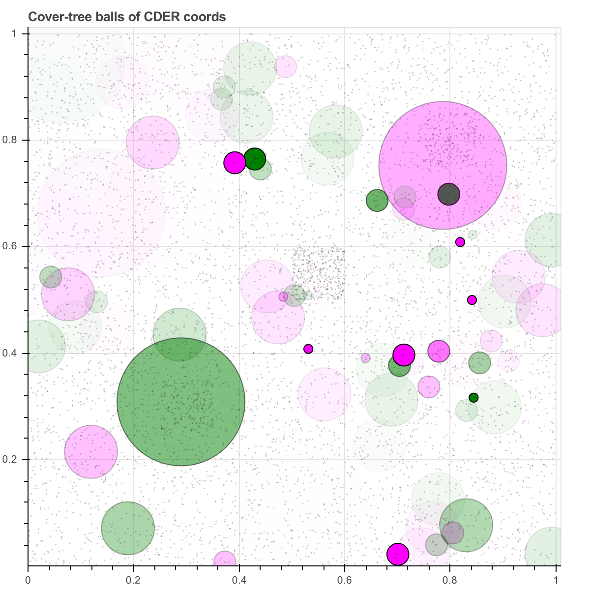
Figure 1. Top: a single magenta pointcloud with 34 points, and a single green pointcloud with 34 points. Bottom: the union of a cloud collection consisting of 100 pointclouds from each label, and CDER identifies the upper-right and lower-left concentrations while mostly ignoring the background and the mutual concentration in the middle.

We analyze the relative density of labels over regions $\Omega$ using the information-theoretic notion of entropy (see Section 5), locating subregions of low entropy. Because of the use of cover trees, our method emphasizes regions $\Omega$ that are very large, very dense, or small-yet-remote (see Section 4). For each of these regions $\Omega$, we construct a function $g$ that approximates $f_{\lambda}$ near $\Omega$; such a $g$ is an example of what we call a distributional coordinate (see Section 3).

2. Weights

Typically, pointclouds are experimental samples that do not come with pre-assigned weights, and we assign weights as follows: We have the prior assumption that each label $\lambda\in\Lambda$ is equally likely among the test data. We give the training set total weight 1. That is, each label is alloted total weight $\frac{1}{L}$, where $L=|\Lambda|$. Moreover, we make the assumption that each sample $X_{i}$ is equally representative of its underlying density function $f_{\lambda_{i}}$, regardless of $|X_{i}|$. That is, each pointcloud $X_{i}$ is alloted total weight $\frac{1}{LN_{i}}$, where $N_{i}$ is the cardinality of ${X}|_{\lambda_{i}}$, the number of training pointclouds with label $\lambda_{i}$. Finally, we assume all points $x\in X_{i}$ have equal weight, so $w(x)=\frac{1}{LN_{i}|X_{i}|}$. Let $\underline{\mathcal{X}}$ denote the labeled and weighted pointcloud given by the union of all $X_{i}$ with these labels and weights.

For example, suppose that the training set consists of $X_{1},X_{2},X_{3}$ where $|X_{1}|=4$, $|X_{2}|=10$, and $|X_{3}|=3$ with labels red, blue, and red, respectively. Suppose we want $\underline{\mathcal{X}}$ to have unit weight. Then each $x\in X_{1}$ has weight $w(x)=\frac{1}{2\cdot 2\cdot 4}=\frac{1}{16}$, each $x\in X_{2}$ has weight $w(x)=\frac{1}{2\cdot 1\cdot 10}=\frac{1}{20}$, and each $x\in X_{3}$ has weight $w(x)=\frac{1}{2\cdot 2\cdot 3}=\frac{1}{12}$.

These weights are chosen to model relative likelihoods in the following way: If each label $\lambda$ has an underlying density function $f_{\lambda}$, and each $X_{i}$ with label $\lambda$ is a sample from $f_{\lambda}$, then $\int_{\Omega}f_{\lambda}$ should be proportional to $\sum_{X_{i}\in\mathcal{X}|_{\lambda}}\sum_{x\in X_{i}\cap\Omega}w(x)$ for any measurable set $\Omega$.

3. Distributional Coordinates

Given a cloud collection $\mathcal{X}$ as above, we would like to map each pointcloud $X$ to a vector $\textbf{v}(X)\in\mathbb{R}^{k}$ for some fixed dimension $k$. While this is an interesting topic in its own right, we are mainly concerned with viewing this as a feature extraction method: that is, the vectors $\textbf{v}_{i}=\textbf{v}(X_{i})\in\mathbb{R}^{k}$ and corresponding labels $\lambda_{i}=\lambda(X_{i})$ will be used as input for any supervised learning algorithm that requires collections of vectors in a common Euclidean space, along with class labels.

One could imagine a supervised learning approach to labeled pointclouds that does not perform feature extraction; for example, by first defining a (non-Euclidean) metric between pointclouds, and then applying a nearest-neighbor or clustering method. However, most such metrics are unstable to noise (such as Hausdorff distance) or are slower-than-linear to compute (such as various Kullback-Leibler Divergence [10] or the Wasserstein metric [9]).

This section frames the problem of feature extraction in the common language of distributional coordinates. We start with a definition of this intuitive concept, and then describe the advantages and disadvantages of some standard examples. The approach we advocate comes in the next section.

Let $g$ be an integrable function on Euclidean space. For any pointcloud $X=\{x_{1},\ldots,x_{|X|}\},$ with pointwise weights $w_{i}=w(x_{i})$, define

$$\int_{X}g=w_{1}g(x_{1})+\ldots+w_{|X|}g(x_{|X|}).$$

We refer to $g$ as a distributional coordinate. Any ordered set $(g_{1},\ldots,g_{k})$ of distributional coordinates transforms $X$ into a vector $\mathbf{v}_{X}=(\int_{X}g_{1},\ldots,\int_{X}g_{k})\in\mathbb{R}^{k}$. It is computationally important to keep the dimension $k$—or at least the intrinsic dimension of $\{\mathbf{v}_{X}~{}:~{}X\in\mathcal{X}\}$—as small as possible, as we hope to minimize the negative effect of the curse of dimensionality on the supervised learning problem.

We use the cloud collection $\mathcal{X}$ shown on the bottom of Figure 2 as a notional working example in the Euclidean plane. There are two class labels, “magenta” and “green.” We imagine that each magenta pointcloud (a typical example on the top-left of the figure) contains a large number of points sampled from a large central blob and a few points sampled from much smaller blobs along the horizontal axis. Each green pointcloud (a typical example on the top-right of the figure) contains a large number of points sampled from the same large central blob and a few points sampled from smaller, different blobs along the horizontal axis.

In a typical supervised learning context, $\mathcal{X}$ would be split (say 80:20) into training and testing sets, and we would build a set of distributional coordinates from the labeled training set which could then infer the correct color labels on the testing set.

3.1. Binning

A simple approach would be to let each $g_{i}$ be the indicator function on some region $R_{i}$; that is, $g_{i}$ takes the value $1$ on some region $R_{i}$ and $0$ elsewhere. Then $\int_{X}g_{i}$ counts the total weight of the points $X\cap R_{i}$. Assuming the regions $R_{1},\ldots R_{k}$ cover the domain with overlap only on boundaries (for example, the $R_{i}$ could be the squares shown in Figure 2) this is what is commonly referred to as binning, and it has been used (for example, [4]) successfully for supervised-learning on labeled pointclouds. On the other hand, binning is obviously unstable: consider a point $x\in X$ that lies very close to the boundary between two adjacent bins. It also can suffer from the curse of dimensionality: a larger number of bins than are shown in Figure 2 would be needed to distinguish the class labels.

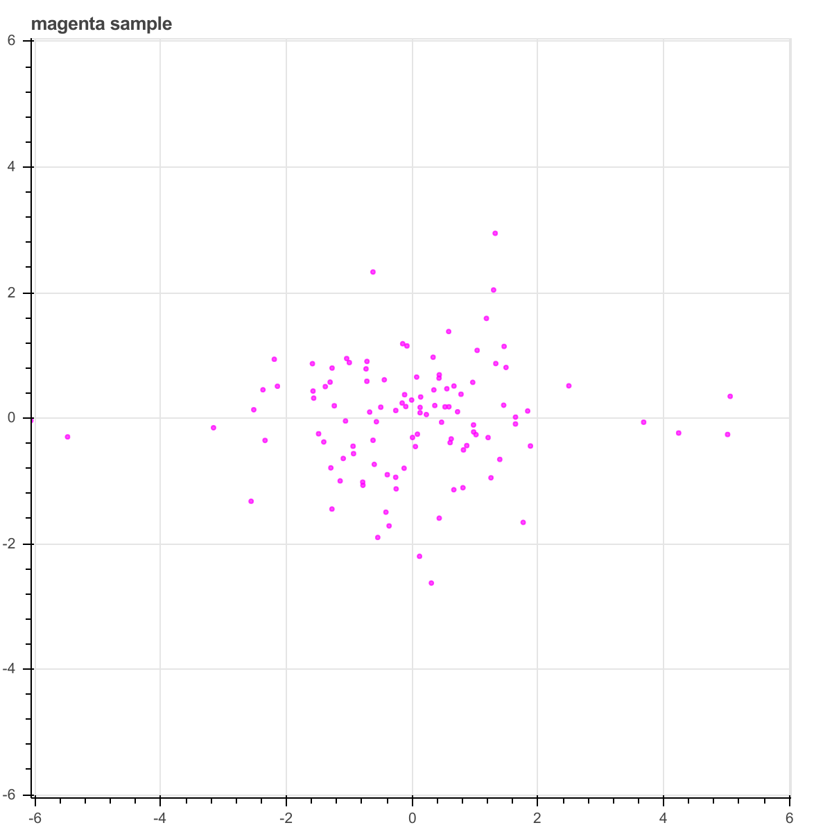
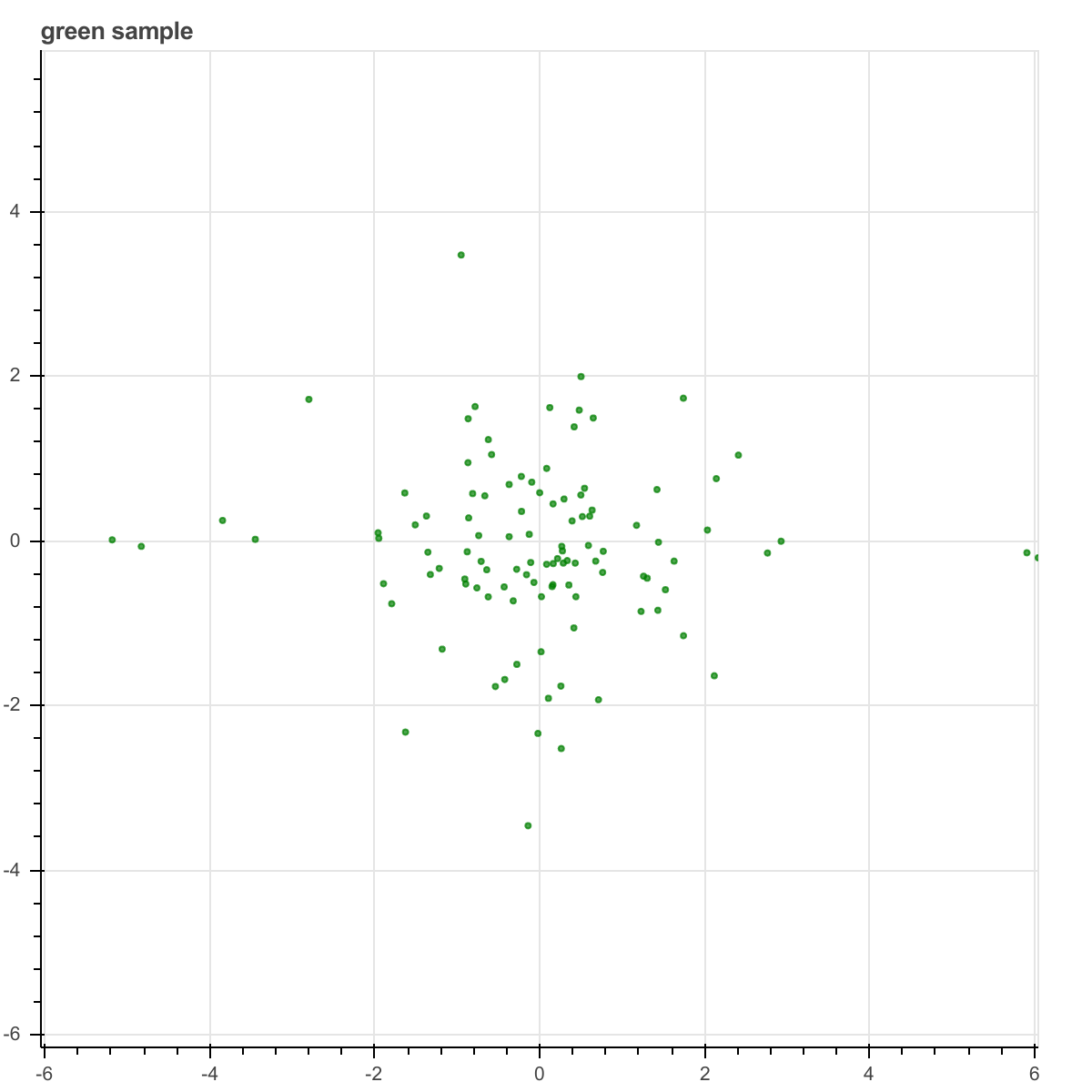
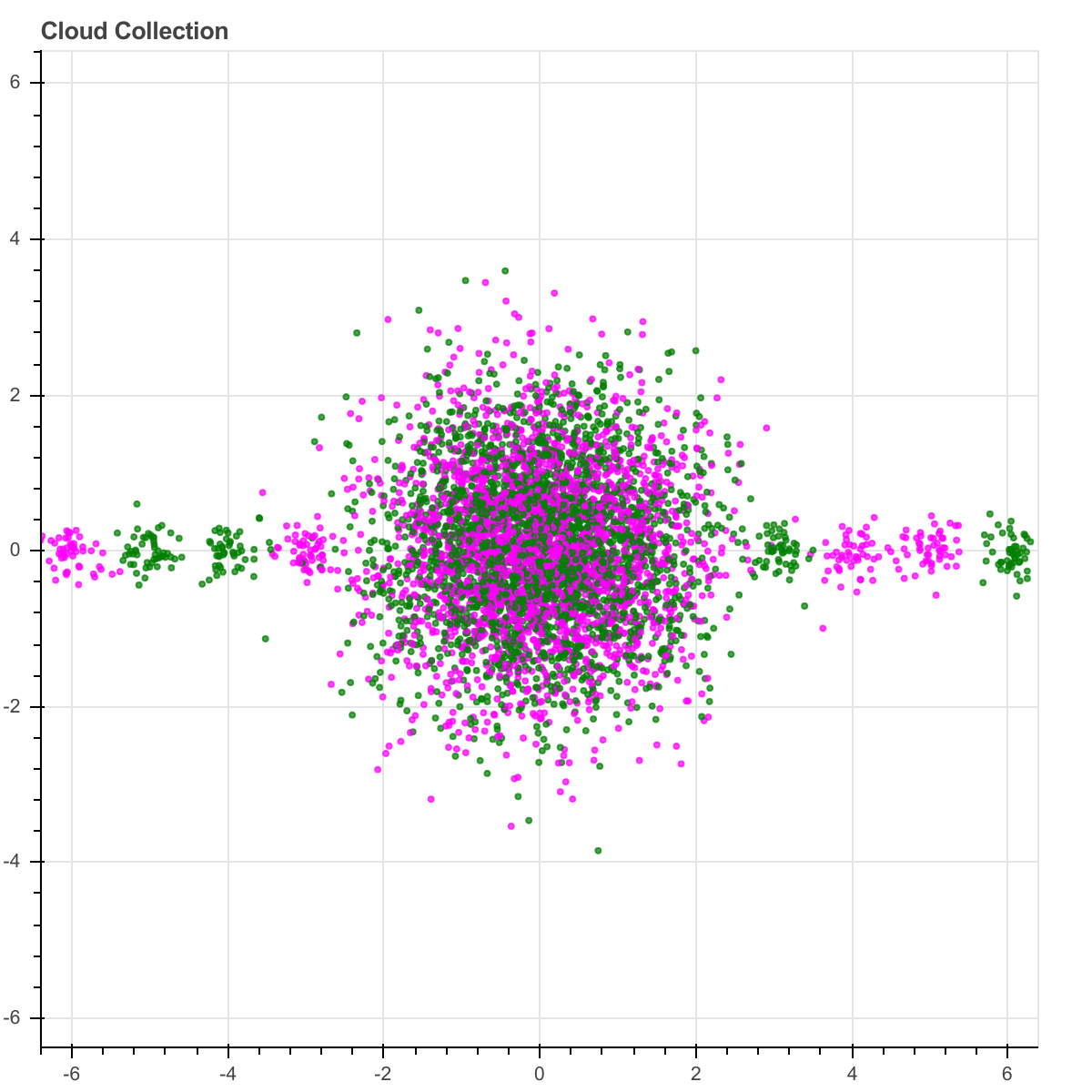
Figure 2. Bottom: a cloud collection of magenta and green point clouds. Top-left: a typical magenta point cloud. Top-right a typical green point cloud.

3.2. Gaussian Mixtures

To address instability, one could define each $g_{i}$ to be a Gaussian with mean $\mu_{i}$ and covariance matrix $\Sigma_{i}$. The obvious questions are: how many Gaussians (modes) should be used, what are their means, and what are their covariances? A data-driven approach should be used to fit a Gaussian Mixture Model ([8], VI.8) to $\underline{\mathcal{X}}$.

It is apparent to the human eye that nine Gaussians (1 large green and magenta, 4 small magenta, and 4 small green) model the example in Figure 2. That is, we could “by hand” define a good set of distributional coordinates to establish a feature vector $\mathbf{v}=(g_{1},\ldots,g_{9}):\mathcal{X}\to\mathbb{R}^{9}$. Moreover, for the purposes of classification, the central “large” distributional coordinate $g_{1}$ is useless. And perhaps the two innermost “small” Gaussians are less useful, as the remaining six distributional coordinates are sufficient for accurate classification. Our goal is to replicate this observation: we construct Gaussian modes $(g_{1},\ldots,g_{k})$ in a data-driven manner from $\underline{\mathcal{X}}$ that are appropriate for use as labeled distributional coordinates for the label classification problem. We now proceed to the computational details.

4. Cover Trees

Cover trees were originally conceived [7] as a way to accelerate the nearest-neighbors problem. More recently, they have been used in dictionary learning [2] and for speeding up the analysis of the topology of pointclouds [13], to pick just a few applications. This section gives basic definitions for cover trees as well as a fast algorithm for their construction; our account is far more detailed than usually appears in the literature and is meant to accompany our publicly available code. Sections 5 and 6 use cover trees to define a set of label-driven distributional coordinates on a cloud collection with class labels.

For any finite pointcloud $\underline{\mathcal{X}}\subset M$, consider a filtration

$$A_{0}\subset\cdots\subset A_{\ell}\subset A_{\ell+1}\subset\cdots\subset\underline{\mathcal{X}}.$$

An element $a\in A_{\ell}$ is called an adult at level $\ell$. The set $A_{\ell}\setminus A_{\ell-1}$ is the cohort at $\ell$.

A cover tree builds a filtration by covering $\underline{\mathcal{X}}$ with balls of smaller and smaller radius centered at the points in $A_{\ell}$. See Figure 3.

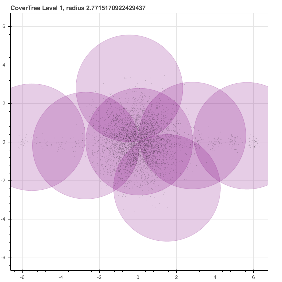
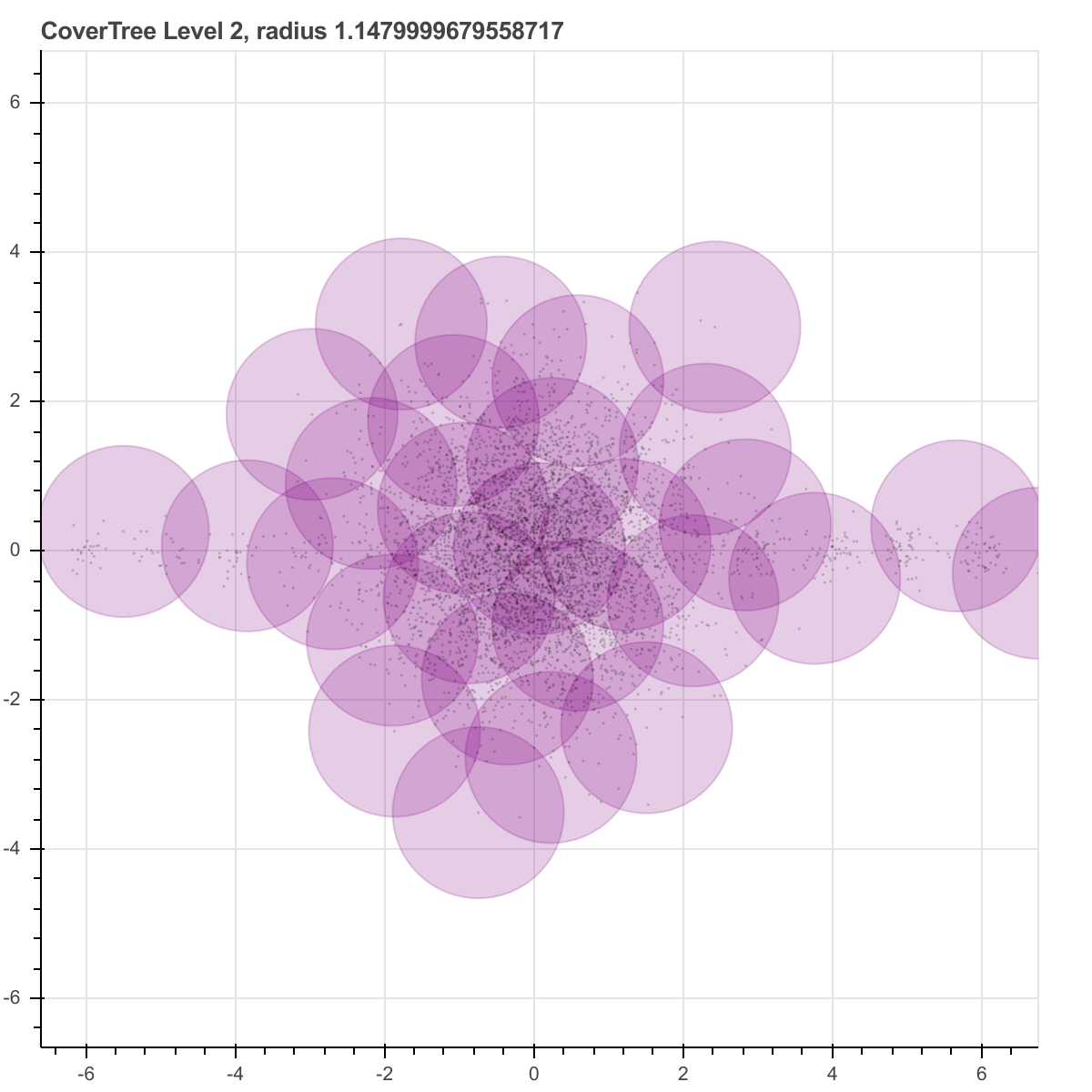
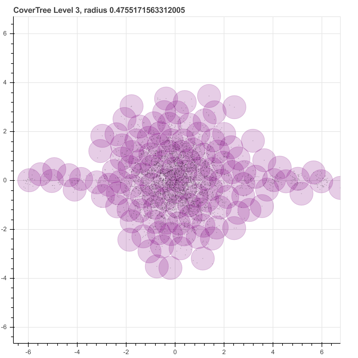
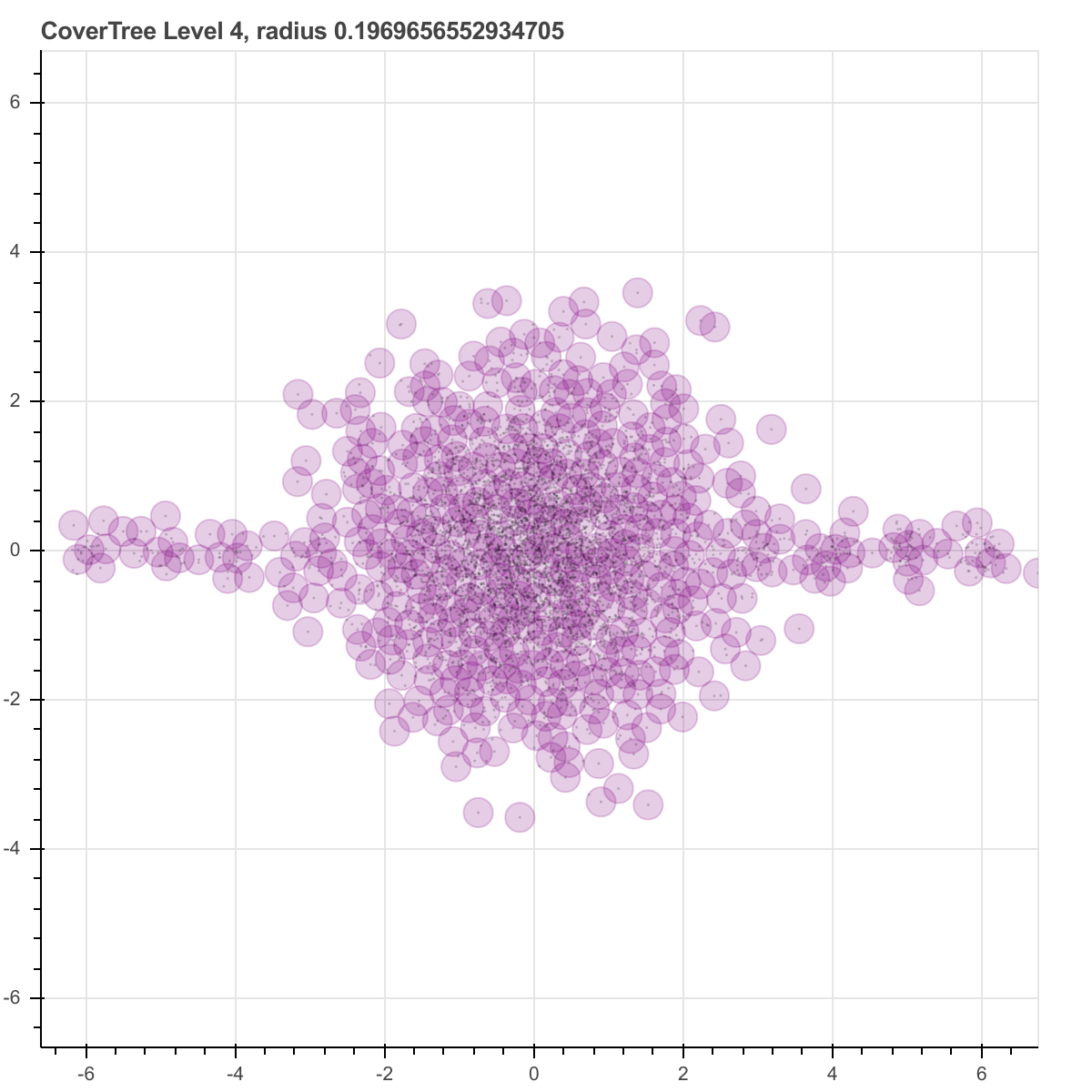
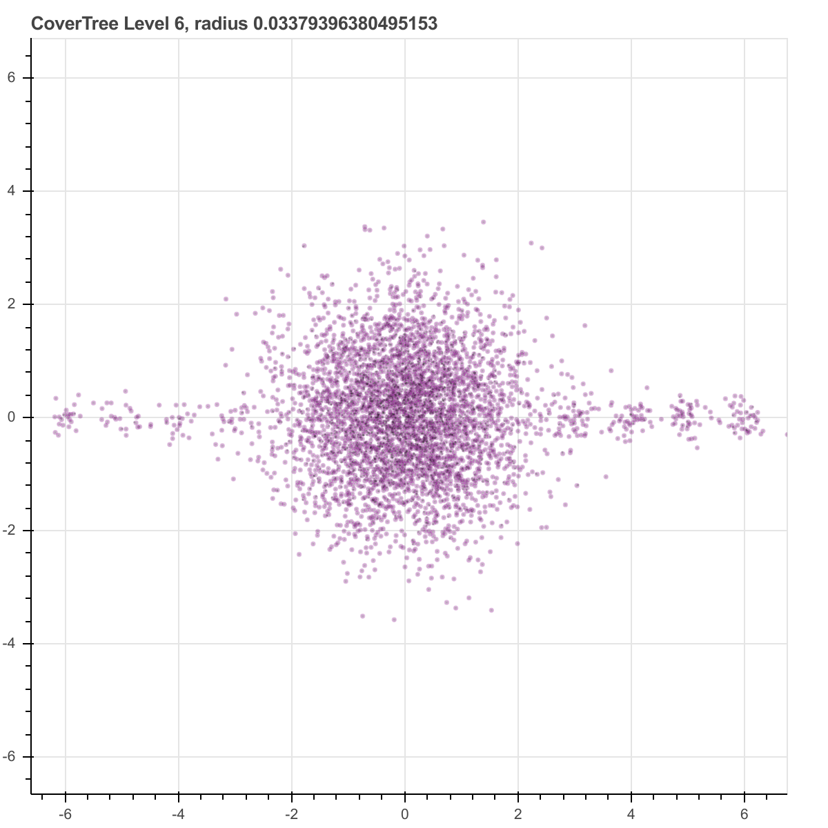
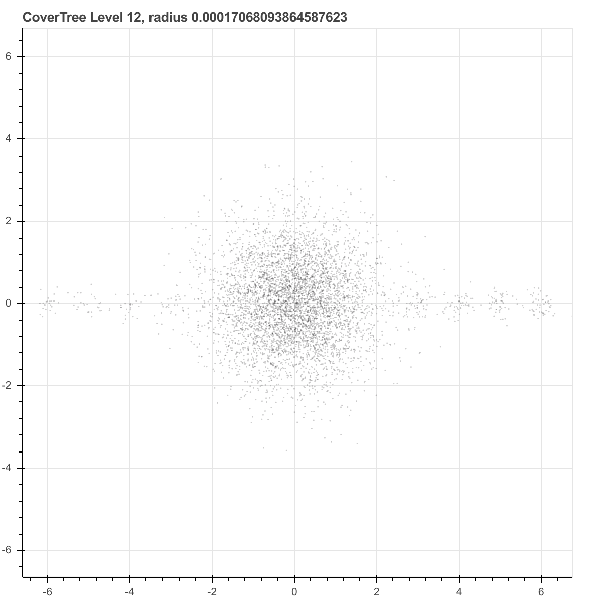
Figure 3. Levels 1, 2, 3, 4, 6, and 12 of a cover tree for the dataset $\underline{\mathcal{X}}$ seen in Figure 2.

Specifically, a cover tree is a filtration of $\underline{\mathcal{X}}$ with the following additional properties:

1. $|A_{0}|=1$. Let $A_{0}=\{a_{0}\}$;

2. There is a radius $r_{0}$ such that $\underline{\mathcal{X}}\subset B(a_{0},r_{0})$;

3. There is a real number $0<\theta<1$, called the shrinkage ratio such that, for every $\ell$, $\underline{\mathcal{X}}\subset\cup_{a_{i}\in A_{\ell}}B(a_{i},r_{\ell})$ where $r_{\ell}=\theta^{\ell}r_{0}$.

4. For each $\ell$, if $a_{i},a_{j}\in A_{\ell}$, then $d(a_{i},a_{j})>r_{\ell}$.

5. For each $\ell$, each point $x\in\underline{\mathcal{X}}$ is assigned to a guardian $a_{i}\in A_{\ell}$ such that $x$ lies in the ball $B(a_{i},r_{\ell})$; we say $x$ is a child of $a_{i}$. Each $a_{i}\in A_{\ell}$ is its own guardian and its own child.

6. There is a tree structure on the (level, adult) pairs of the filtration $(\ell,a_{i})$, where there is a tree relation $(\ell,a_{i})\to(\ell+1,a_{k})$ if $a_{k}$ was a child of $a_{i}$ at level $\ell$. We say $a_{k}$ is a successor of $a_{i}$, and $a_{i}$ is a predecessor of $a_{k}$. Note that $(\ell,a_{i})\to(\ell+1,a_{i})$ for all $a_{i}\in A_{\ell}$.

4.1. Vocabulary

Cover trees can be generated using a fast algorithm relying on the notion of friends, first introduced in [7]. The rough algorithm is familiar to many practitioners, but is not widely published. We enhance this algorithm by giving each point a weight and a label. We describe our method here because the details of the construction are crucial to the supervised-learning task of this article.

Extending the maturation/reproduction metaphor of adults, children, and guardians above, a child $x$ with guardian $a_{i}$ at level $\ell$ is called a teen if $\frac{1}{2}r_{\ell}<d(a_{i},x)$, and it is called a youngin if $d(a_{i},x)\leq\frac{1}{2}r_{\ell}$. See Figure 4. When changing from level $\ell$ to level $\ell+1$, the radius of each ball shrinks to $r_{\ell+1}=\theta r_{\ell}$. Children farther than $r_{\ell+1}$ from their guardians become orphans. We must decide whether these orphans should be adopted by other adults at level $\ell+1$, or if the orphans should be emancipated as new adults at level $\ell+1$. That is, the newly emancipated adults at level $\ell+1$ comprise the cohort at level $\ell+1$.

Our algorithm uses several notions of friends, set by the following bounds at level $\ell$:

(1) $$\begin{split}T_{1}(\ell)&=(2+\theta)r_{\ell},\\ T_{2}(\ell)&=(2+2\theta)r_{\ell},\\ T_{3}(\ell)&=2(1+\theta+\theta^{2}+\cdots)r_{\ell}=\frac{2}{1-\theta}r_{\ell}.\end{split}$$

For each $k=1,2,3$, we say that adults $a_{i}$ and $a_{j}$ at level $\ell$ are type-$k$ friends if $d(a_{i},a_{j})\leq T_{k}(\ell)$. It is easy to verify the following recursion relations:

(2) $$\begin{cases}T_{1}(\ell)\leq T_{2}(\ell)\leq T_{3}(\ell),\\ T_{1}(\ell+1)\leq T_{1}(\ell),\\ T_{2}(\ell+1)\leq T_{2}(\ell),\\ T_{3}(\ell+1)\leq T_{3}(\ell).\\ \end{cases}$$

Figure 4. The relevant radii for the special ratios $\theta=\sqrt{2}-1$, $\theta=1/2$, and $\theta=(\sqrt{5}-1)/2$. The orange ball has radius $r_{\ell}$. The red ball has radius $r_{\ell+1}$. The small dotted sphere separates youngins from teens. The larger dashed sphere contains the elders.

Figure 5. An orphan $x$ of $a_{i}$ could potentially be adopted by a successor of $a_{j}$ if $d(a_{i},d_{j})\leq T_{1}$.

Figure 6. A teen $x$ of $a_{k}$ at level $\ell+1$ could be exchanged to some $a_{h}$, where the distance between the level-$\ell$ predecessors of $a_{k}$ and $a_{h}$ is at most $T_{2}(\ell)$.

Figure 7. If two adults are type-3 friends at level $\ell+1$, then their predecessors are type-3 friends at level $\ell$.

Figure 8. $a_{j}$ is an elder of $a_{k}$ if a level-$(\ell+1)$ child of $a_{k}$ could potentially have been a level-$\ell$ child of $a_{j}$.

Here are the essential facts about friends, which are immediate consequences of the triangle inequality:

Theorem 1.

1. If $x$ is a child of $a_{i}$ at level $\ell$ that is orphaned at level $\ell+1$, then $x$ can be adopted only by either the type-1 friends of $a_{i}$ at level $\ell$ or the newly-emancipated children at level $\ell+1$ of those type-1 friends. See Figure 5.

2. If we choose to re-assign children to the nearest adult, then teen $x$ with guardian $a_{k}$ can be adopted by adult $a_{h}$ at level $\ell+1$, where the level-$\ell$ predecessors of $a_{k}$ and $a_{h}$ are type-2 friends. See Figure 6.

3. If $a_{k}$ and $a_{h}$ are type-3 friends at level $\ell+1$, then their predecessors $a_{i}$ and $a_{j}$ are type-3 friends at level $\ell$. See Figure 7.

Theorem 2.

Suppose $a_{k}$ is an adult at level $\ell{+}1$ with predecessor $a_{i}$. If $x$ has guardian $a_{k}$ at level $\ell{+}1$ and guardian of $a_{j}$ at level $\ell$, then $a_{j}$ is a type-1 friend of $a_{i}$, and $d(a_{k},a_{j})\leq r_{\ell}+r_{\ell+1}=\frac{1}{2}T_{2}(\ell)$. See Figure 8.

Based on this scenario, we say $a_{j}\in A_{\ell}$ is an elder of $a_{k}\in A_{\ell+1}$ if $d(a_{k},a_{j})\leq\frac{1}{2}T_{2}(\ell)$. Moreover, if $a_{i}=a_{k}$ is its own predecessor, then $a_{j}=a_{i}=a_{k}$ is its only elder, so the notion of elder is nontrivial only if $a_{k}$ belongs to cohort $\ell$.

Theorem 3.

For the purpose of computing elders, there are three particularly good choices of $\theta$ which require no additional computation. If $\theta=\frac{1}{2}(\sqrt{5}-1)$, then $\frac{1}{2}T_{2}(\ell)=T_{1}(\ell+1)$. If $\theta=\frac{1}{2}$, then $\frac{1}{2}T_{2}(\ell)=T_{2}(\ell+1)$. If $\theta=\sqrt{2}-1$, then $\frac{1}{2}T_{2}(\ell)=T_{3}(\ell+1)$. In these cases, the elders of $a_{k}$ are the friends (of the respective type) $a_{j}$ that have cohort $\ell$ or less. See Figure 4.

These facts allow the following algorithm.

4.2. Algorithm

At level $0$, the cover tree has a single adult, $a_{0}$. All points are its children. Its only friend is itself. Every $x\in\underline{\mathcal{X}}$ has some weight and some label, which we assume as given input. For each label $\lambda$, compute the total weight and weighted mean of all children of $a_{0}$ with that label.

Suppose at level $\ell$, the friends, children, per-label weights, and per-label means are known for all adults $a_{i}\in A_{\ell}$. We compute these for level $\ell+1$ as follows:

• Advance. Shrink the radius by a factor of $\theta$ to $r_{\ell+1}=r_{\ell}\theta$. Every adult $a_{i}\in A_{\ell}$ remains an adult $a_{i}\in A_{\ell{+}1}$. Mark $a_{i}$ as its own elder.

• Orphan. For each $a_{i}\in A_{\ell}$, find its orphaned children: those $x$ such that $d(a_{i},x)>r_{\ell+1}$. Sort the orphans so that the first orphan is the one nearest the per-label mean for the label of greatest weight, the second orphan is the one nearest the per-label mean of the label of second-greatest weight, and so on, via a two-dimensional argsort without repetition. The reason for this sorting will become apparent in Section 6.

• Adopt or emancipate. For each $a_{i}\in A_{\ell}$, consider its orphans in order. For each $x$ orphaned by $a_{i}$, check whether $x$ can be adopted by another adult using the type-1 friends of $a_{i}$:

  • If so, the adoptive guardian will be a adult $a_{h}$ such that $d(a_{h},x)\leq r_{\ell+1}$. The predecessor $a_{j}$ of $a_{h}$ has $d(a_{j},a_{i})\leq T_{1}(l)$.

  • If not, then $x$ is a new adult at level $\ell+1$. Its only child is itself. Its friends are initialized to be itself and its predecessor $a_{i}$ (but these will be updated in the Befriending stage). Note the set $A_{\ell+1}$ is ordered by cohort, and within a cohort is ordered by predecessor, and within a predecessor block is ordered by proximity to the predecessor’s per-label means.

• Exchange Teens. If $x$ has guardian $a_{i}$, then check whether it is closer to some other guardian using type-2 friends. That is, find $a_{h}=\operatorname{argmin}_{A_{\ell+1}}d(x,\cdot)$. The predecessor $a_{j}$ of $a_{h}$ has $d(a_{j},a_{i})\leq T_{2}(\ell)$. Note that $a_{h}\neq a_{i}$ implies $d(a_{h},x)>\frac{1}{2}r_{\ell+1}$, meaning that only teens (not youngins) can be exchanged.

• Befriend: Now, all $(\ell+1)$-adults and their children are known. We need to find new friends using the recursion relation and the predecessors.

  • A pair of $\ell+1$ adults, $a_{k}$ and $a_{h}$, are type-3 friends if their predecessors $a_{i}$ and $a_{j}$ are type-3 friends at level $\ell$ and $d(a_{k},a_{h})\leq T_{3}(\ell+1)$.

  • A pair of $\ell+1$ adults, $a_{k}$ and $a_{h}$, are type-2 friends if they are type-3 friends and $d(a_{k},a_{h})\leq T_{2}(\ell+1)$.

  • A pair of $\ell+1$ adults, $a_{k}$ and $a_{h}$, are type-1 friends if they are type-2 friends and $d(a_{k},a_{h})\leq T_{1}(\ell+1)$.

  • For each newly emancipated adult $a_{k}$ of cohort $\ell+1$, find its elders by searching its friends for elements of cohort $\ell$ or less.

• Weigh: For each adult $a_{k}$ at level $\ell+1$, compute the per-label weights and per-label weighted means for its children. Sort the labels by their weights from greatest to least.

At level $\ell{+}1$, the friends, children, per-label weights, and per-label means are all known.

4.3. Algorithmic Efficiency

Suppose $n=|\underline{\mathcal{X}}|$, and the cover-tree filtration stops at level $\ell_{\text{max}}$. We are interested in the storage and computational complexity of this algorithm in terms of $n$, for a fixed ambient dimension $D$.

The desired output is the successor/predecessor tree and the children/guardian relationships at each level. Thus, storage of friend lists is the only issue that might lead us to another algorithm. The main question is: given an adult $a_{i}$ at level $\ell$, how many other adults are within $T_{3}(\ell)=\frac{2}{(1-\theta)}r_{\ell}$ of $a_{i}$?

Since no two adults at level $\ell$ are within $r_{\ell}$ of one another, this is related to the idea of “doubling dimension.” Define $\mathbb{D}(D,\alpha)$ to be the maximum number of points in $\mathbb{R}^{D}$ that can be placed in the ball of radius $\alpha$, including the center, so that no two points have distance $\leq 1$. This number grows with the ambient dimension $D$. In Euclidean space, it is independent of scale; that is, the same number works for a ball of radius $r\alpha$ using points of distance at least $r$. The number can be bounded by the number of simplices with edge length at least $1$ that can be put into a ball of radius $\alpha$. Since these simplices have a minimum volume $\frac{\sqrt{D+1}}{D!2^{D/2}}$, we get a bound like:

$$\mathbb{D}\leq\operatorname{Vol}(B_{\alpha})\frac{D!2^{D/2}}{\sqrt{D+1}}\sim\frac{D!(\alpha)^{D}(2\pi)^{D/2}}{(\frac{D}{2})!\sqrt{D+1}}\sim O(D!2^{D}\alpha^{D}).$$

Setting $\alpha=\frac{2}{1-\theta}$, we get an upper bound on the expected size of the friends list, which is a constant independent of the level $\ell$. Thus, the total storage size is $O(n)$; in particular, it is at most $3\mathbb{D}n$, where the $3$ accounts for the lists of type-1, type-2, and type-3 friends.

Setting $\alpha=\frac{1}{\theta}$, we get an upper bound on the expected number of successors of an adult from level $\ell$ to $\ell+1$, which is a constant independent of the level $\ell$. The size of $A_{0}$ is $|A_{0}|=1$. The maximum expected size of $A_{1}$ is $\mathbb{D}$. The maximum expected size of $A_{2}$ is $\mathbb{D}^{2}$. Generally, the maximum expected size of $A_{\ell}$ is $\mathbb{D}^{\ell}$. Moreover, the larger the size of each cohort $A_{\ell}\-A_{\ell-1}$, the shallower the cover tree. That is, $\ell_{\text{max}}$ is expected to be of the order $\log_{\mathbb{D}}(n)$.

For each adult $a_{i}\in A_{\ell}$, we must:

1. Sum and sort the weights of its children, by label. The expected number of children is $n/\mathbb{D}^{D}$. Sorting the labels is $O(L\log(L))$ for $L$ labels.

2. Compute the distance (an $O(D)$ operation) to each of its roughly $\theta^{\ell}n$ children. These distances yield the orphans and teens. The expected number of orphans is $(1-\theta^{D})\frac{n}{\mathbb{D}^{\ell}}$, and the expected number of teens is $\left(1-(\frac{1}{2})^{D}\right)\frac{n}{\mathbb{D}^{\ell}}$.

3. For each orphan, determine whether it should be adopted or liberated. Compute the distance (an $O(D)$ operation) to the $T_{1}$ friends or successors of the $T_{1}$ friends of $a_{i}$. This set has expected size $\mathbb{D}^{2}$, which is constant in $n$.

4. For each teen, determine whether it should be exchanged. Compute the distance (an $O(D)$ operation) to the $T_{2}$ friends or successors of the $T_{2}$ friends of $a_{i}$. This set has expected size $\mathbb{D}^{2}$, which is constant in $n$.

5. For each successor—a list of size $\mathbb{D}$—update its friends by computing the distance (an $O(D)$ operation) to the successors of the $T_{3}$ friends of $a_{i}$. This is expected to be $\mathbb{D}^{2}$ distance computations.

For each adult at level $\ell$, this is roughly $\frac{n}{\mathbb{D}^{\ell}}$ operations, albeit with an additional penalty from $D$. Level $\ell$ has at most $\mathbb{D}^{\ell}$ adults, in which case the total number of computations is roughly

$$\sum_{\ell=0}^{\ell_{\text{max}}}\mathbb{D}^{\ell}\frac{n}{\mathbb{D}^{\ell}}O(\mathbb{D}^{2})\sim O(n\log_{\mathbb{D}}n)O(\mathbb{D}^{2}).$$

It is interesting that the rapid growth from the ambient dimension $D$ is counteracted by the logarithm term. In our experience with applications, this is effectively linear in $n$, as the sum terminates earlier than this estimate. This is because the estimate of $\ell_{\text{max}}$ by $\log_{\mathbb{D}}(n)$ is typically irrelevant; the maximum level $\ell_{\text{max}}$ of the cover tree is actually controlled by the ratio of the maximum to the minimum distances in the pointcloud. In applications, these are typically within several orders of magnitude, so with $\theta=\frac{1}{2}$, we expect $\ell_{\text{max}}\sim 14$. Moreover, in our supervised-learning application in Section 6, we abort the cover tree much earlier, once the low-entropy regions have been found.

5. Entropy Reduction

For each label $\lambda$, let $\underline{\mathcal{X}}|_{\lambda}$ denote the (weighted) points in $\underline{\mathcal{X}}$ that have label $\lambda$. For any convex, compact $\Omega$, let $\Omega_{\lambda}=\Omega\cap\underline{\mathcal{X}}|_{\lambda}$. The total weight in $\Omega$ of each label is $w_{\lambda}=\sum\{w(x)~{}:~{}x\in\Omega_{\lambda}\}$, which by Section 2 corresponds to the relative likelihood of a point with label $\lambda$ being sampled from $\Omega$. Let $W=\sum_{\lambda}w_{\lambda}$.

To quantify the relative prominence of the various labels, we use the information-theoretic notion of entropy. Entropy is characterized by several nice properties, detailed in [3]. The formula is

(3) $$\begin{split}S(\Omega)&=-\sum_{\lambda}\frac{w_{\lambda}}{W}\log_{L}\left(\frac{w_{\lambda}}{W}\right)\\ &=-\frac{1}{W}\sum_{\lambda}w_{\lambda}\log_{L}\left(w_{\lambda}\right)+\log_{L}(W).\end{split}$$

If all weights are roughly equal, then entropy is 1. If one label has high weight and the others have weight 0, then the entropy is 0. Generally, entropy decreases as a smaller subset of labels becomes more likely. Thus, low entropy is a good indicator that the region $\Omega$ is particularly prominent for a small subset of labels. The question remains: how can we locate low-entropy regions?

Our search for low-entropy regions is motivated by the following elementary theorems; however, we do not insist that these strict regularity hypotheses hold for any given application.

Theorem 4.

Fix a function $f:\mathbb{R}^{D}\to\mathbb{R}$ that is continuous on a compact, convex set $\Omega$. Fix a radius $r>0$. Let $\mu_{r}(x)$ denote the centroid of $f$ on the compact, convex set $\Omega\cap B_{r}(x)$ (the closed ball). There exists $x\in\Omega$ such that $\mu_{r}(x)=x$.

Proof: Note that $\mu_{r}(x)$ varies continuously with $x$, and apply Brouwer’s fixed-point theorem ([11], II.22).

Theorem 5.

Suppose that $f:\mathbb{R}^{D}\to\mathbb{R}$ is an analytic function with local max at $x$. For any $\epsilon>0$, there exists a radius $r$ such that the centroid $\mu_{r}(x)$ of $f$ on $B_{r}(x)$ has $d(\mu_{r}(x),x)<\epsilon$.

Proof: Expand $f$ as a power series around $x$, and approximate $f$ by truncating at the second-order term. The level sets are concentric ellipsoids about $x$, as given by the positive-definite symmetric matrix $f^{\prime\prime}$.

Theorem 6.

Suppose $f$ and $\tilde{f}$ are positive, continuous functions defined on a compact, convex region $\Omega\subset\mathbb{R}^{D}$. Suppose that $f$ achieves a local max $f(x)=M$ on $\Omega$ and that $\tilde{f}(x)\leq\varepsilon$ on $\Omega$, with $\varepsilon<M$. Then, there is a radius $r$ such that the average value of $f$ on $\Omega\cap B_{s}(x)$ is greater than the average value of $\tilde{f}$ on $\Omega\cap B_{s}(x)$ for all $s\leq r$.

Proof: The mean value theorem for integrals.

Putting these together, we try to find a region $\Omega$ and a ball of radius $r_{\ell}$ in that region whose center is near the mean of a particular label. We ask whether the entropy of that ball is non-decreasing with radius; that is, does the entropy become lower (or remain the same) when the ball shrinks? If true, this is consistent with the hypothesis that a local maximum of a particular label occurs near the center of that ball, while other labels remain roughly constant. If false, then we subdivide the region and search around the boundary of the original ball for other smaller regions of low entropy.

Specifically, the compact, convex regions corresponds to the children of an adult $a_{i}\in A_{\ell}$ in the cover tree, and the sub-balls correspond to the children of successors of $a_{i}$ at level $\ell+1$ in the cover tree. This is the heart of the CDER algorithm in Section 6.

6. Cover-tree Differencing via Entropy Reduction

The input data is a ratio $\theta$ and a training set of pointclouds $X_{1},X_{2},\ldots,X_{N}$ with labels $\lambda_{1},\lambda_{2},\ldots,\lambda_{N}$, respectively. Set weights as in Section 2.

6.1. Region Selection

Here we describe the heart of the CDER algorithm, wherein we search the adults of the cover tree as a data-driven method to locate regions on which we want to build distributional coordinates. The construction and weighting of those distributional coordinates occurs in Section 6.2.

For each level of the cover tree, define a subset $\hat{A}_{\ell}\subset A_{\ell}$ of adults that are still potential candidates for distributional coordinates. Set $\hat{A}_{0}=A_{0}=\{a_{0}\}$. Once $\hat{A}_{\ell}=\{\}$, we break.

The cover tree of $\underline{\mathcal{X}}$ is constructed level-by-level as in Section 4.2. At each level $\ell$ of the cover tree (until break), we perform the following computation:

For each adult $a_{i}\in A_{\ell}$, let $\beta_{\ell}(i)$ denote the set of children of $a_{i}$ at level $\ell$. Let $\alpha_{\ell}(i)=\beta_{\ell+1}(i)$ denote the set of children of $a_{i}$ at level $\ell+1$. Let $\gamma_{\ell}(i)$ denote the union of the children (at level $\ell-1$) of the elders of $a_{i}$. (If $a_{i}$ belongs to cohort $\ell-1$ or less, then $\gamma_{\ell}(i)=\beta_{\ell-1}(i)$.) Note that $\alpha_{\ell}(i)\subset\beta_{\ell}(i)\subset\gamma_{\ell}(i)$; see Figure 9. Then, we decide what to do with $a_{i}$:

Figure 9. The nested sets $\alpha_{\ell}(i)\subset\beta_{\ell}(i)\subset\gamma_{\ell}(i)$ on which we compare entropy. On left, $a_{i}$ has cohort $<\ell$ and is its own elder. On right, $a_{i}$ has cohort $\ell$, and has several elders as in Theorem 2. If the smaller regions have lower entropy, then we build a distributional coordinate using $a_{i}$ at level $\ell$.

• if $\hat{A}_{\ell}=\emptyset$, then break. Nothing more is needed.

• for each adult $a_{i}\in\hat{A}_{\ell}$:

  • if $a_{i}$ has only one child (itself) at level $\ell+1$, then pass. This region is useless.

  • elif $a_{i}$ has only one child (itself) at level $\ell$, then pass. This region is useless.

  • elif $S(\alpha)\leq S(\beta)\leq S(\gamma)<1$, then build a distributional coordinate using the children of $a_{i}$ of each of the dominant labels.

  • elif $S(\gamma)\leq S(\alpha)\leq S(\beta)<1$, then append $a_{i}$ to $\hat{A}_{\ell+1}$. The smaller ball $B(a_{i},r_{\ell+1})$ may contain a lower-entropy region.

  • elif $S(\beta)\leq S(\alpha)\leq S(\gamma)<1$, then append the successors of $a_{i}$—other than itself!—to $\hat{A}_{\ell+1}$. The annulus $B(a_{i},r_{\ell})\setminus B(a_{i},r_{\ell+1})$ may contain a lower-entropy region.

  • elif $S(\beta)\leq S(\gamma)\leq S(\alpha)<1$, then append the successors of $a_{i}$—other than itself!—to $\hat{A}_{\ell+1}$. The annulus $B(a_{i},r_{\ell})\setminus B(a_{i},r_{\ell+1})$ may contain a lower-entropy region.

  • elif $S(\gamma)\leq S(\alpha)\leq S(\beta)<1$, then pass. The region $B(a_{i},r_{\ell})$ is useless.

  • elif if $S(\gamma)\leq S(\beta)\leq S(\alpha)<1$, then pass. The region $B(a_{i},r_{\ell})$ is useless.

  • else (meaning $\max\{S(\alpha),S(\beta),S(\gamma)\}=1$) append the successors of $a_{i}$ to $\hat{A}_{\ell+1}$. There is too little information to decide whether $B(a_{i},r_{\ell})$ contains a low-entropy region, so re-analyze everything at the next level.

Recall that our method in Section 4.2 produces the list $A_{\ell}$ which is ordered by cohort, and within a cohort is ordered by predecessor, and within a predecessor block is ordered by proximity to the predecessor’s per-label means. Therefore, if $a_{i}<a_{j}$ in this ordering, then $a_{i}$ tends to be nearer the mean of the most prominent label of a larger region than $a_{j}$. Hence, the distributional coordinates are sorted by “granularity,” from coarse to fine.

In some scenarios, detailed analysis of clusters is more important than efficient classification. Therefore, one can implement a “non-parsimonious” version by replacing all pass operations with append. For machine learning applications, the “parsimonious” version is far faster, as the cover tree can be stopped much earlier than the limit suggested in Section 4.3.

6.2. Build Distributional Coordinates

For each $a_{i}\in A_{\ell}$ selected to build, we construct a distributional coordinate $g_{i}$ in the following way.

For each of the dominant labels $\lambda$ among the children of $a_{i}$, use PCA/SVD to build a Gaussian model $g_{i,\lambda}$ of mass 1. Let $\Delta S$ denote the entropy difference on $\beta_{\ell}$ caused by erasing the non-dominant labels. We amplify (or attenuate) each Gaussian model by the coefficient

$$m_{i}=w_{\lambda}(1-\Delta S)\left(r_{\ell}\right)^{D}.$$

The distributional coordinate is $m_{i}g_{i,\lambda}(x)$.

One can experiment with different weighting systems; we have found these to be generally effective, and we justify this choice for the following geometric reasons:

• The weight represents the relative likelihood that a point of the given label was selected from the region on which this coordinate was detected. Perhaps, by chance in our selection process, a single region was detected at a later level in the form of several smaller regions. The weight of the smaller regions will sum to the weight of the larger region.

• The entropy term is the “certainty” with which this region was selected. The entropy $\Delta S$ is the information that is lost if the other labels are removed from the region, so $1-\Delta S$ is the information that remains. In other words, this term penalizes regions according to the impurity of their labels.

• The $(r_{\ell})^{D}=(r_{0}\theta^{\ell})^{D}$ term accounts for the relative remoteness of the sample region. All else being equal, remote regions are particularly distinctive. Because of the cover-tree construction, remoteness can be measured by the size of the cover-tree ball. For example, suppose that two different regions are detected by CDER, each with the same entropy, weight, and configuration of points; the Gaussian coordinates are translates of one-another. Suppose that the first region is very distant from the rest of the pointcloud, so it is detected at an early level $\ell$. Suppose that the second region is surrounded closely by other data, so it is not detected by the cover tree until a later level $\ell^{\prime}>\ell$. The first region’s relative volume is $\theta^{(\ell-\ell^{\prime})D}$.

7. Examples

This section illustrates the promise of CDER on several synthetic examples of varying levels of complexity that are designed to stress certain features of the algorithm.

7.1. Blobs

This example shows that CDER ignores high-density regions unless they have low entropy.

Consider two labels: 0/magenta and 1/green. The cloud collection has 25 pointclouds of each label. Each magenta pointcloud consists of:

• 100 points sampled from a standard normal distribution

• 2 points sampled from a normal distribution with $\sigma=0.2$ and mean $(4,0)$

• 2 points sampled from a normal distribution with $\sigma=0.2$ and mean $(5,0)$

• 2 points sampled from a normal distribution with $\sigma=0.2$ and mean $(-3,0)$

• 2 points sampled from a normal distribution with $\sigma=0.2$ and mean $(-6,0)$

Each green pointcloud consists of

• 100 points sampled from a standard normal distribution

• 2 points sampled from a normal distribution with $\sigma=0.2$ and mean $(-4,0)$

• 2 points sampled from a normal distribution with $\sigma=0.2$ and mean $(-5,0)$

• 2 points sampled from a normal distribution with $\sigma=0.2$ and mean $(3,0)$

• 2 points sampled from a normal distribution with $\sigma=0.2$ and mean $(6,0)$

This produces the cloud collection in Figure 2. The output of CDER appears in Figure 10

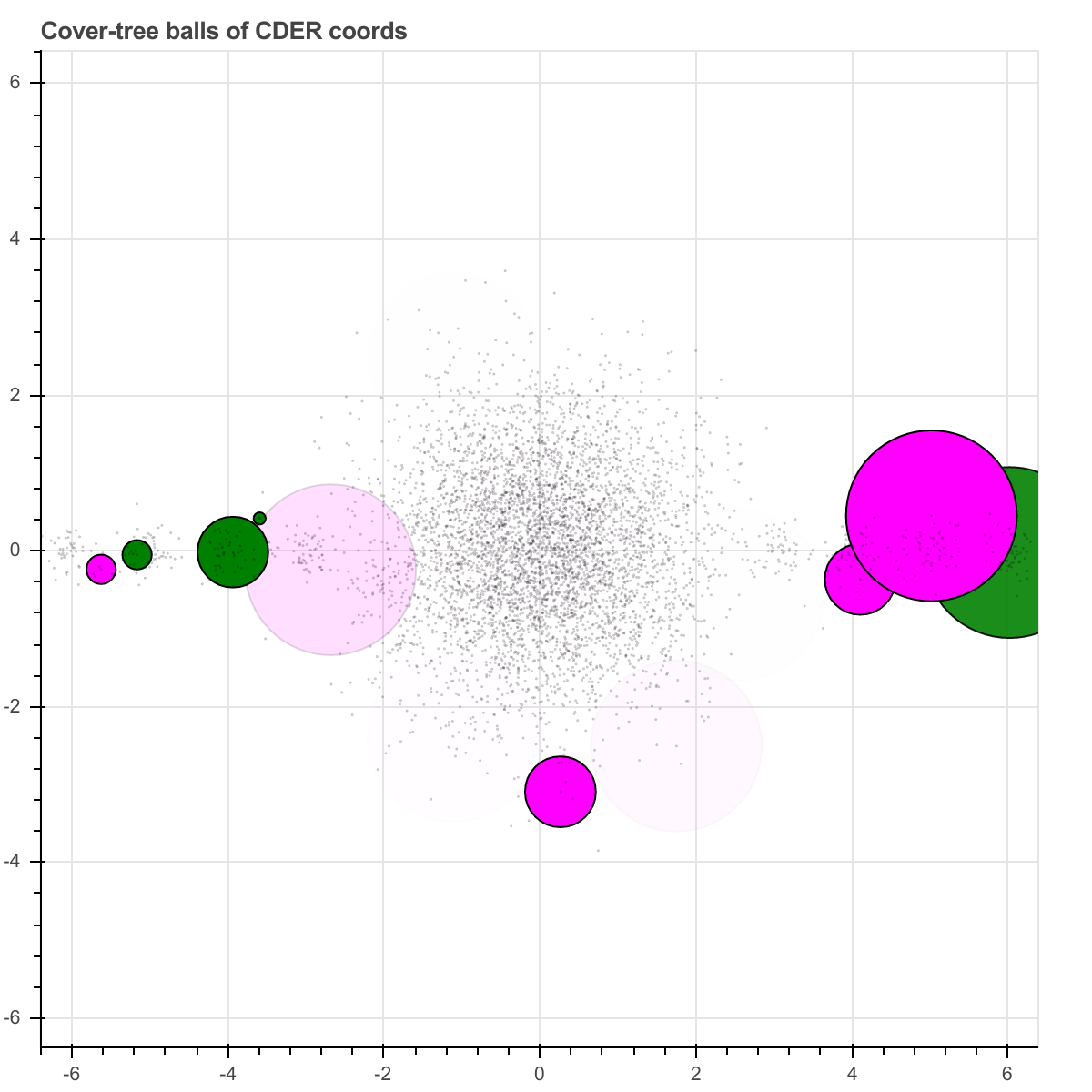
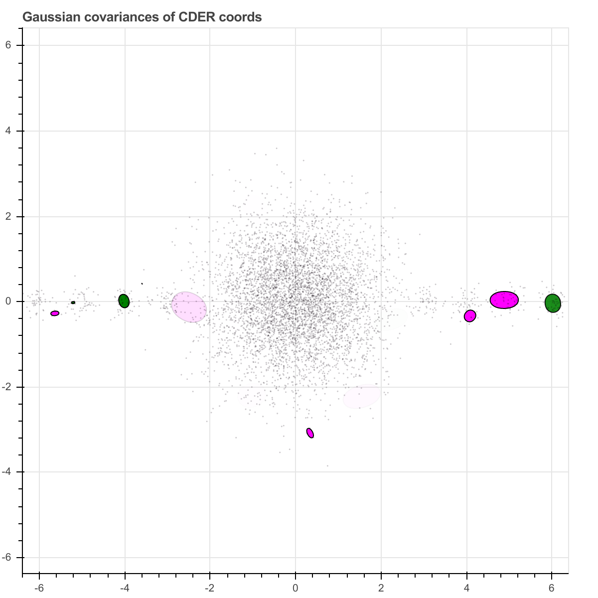
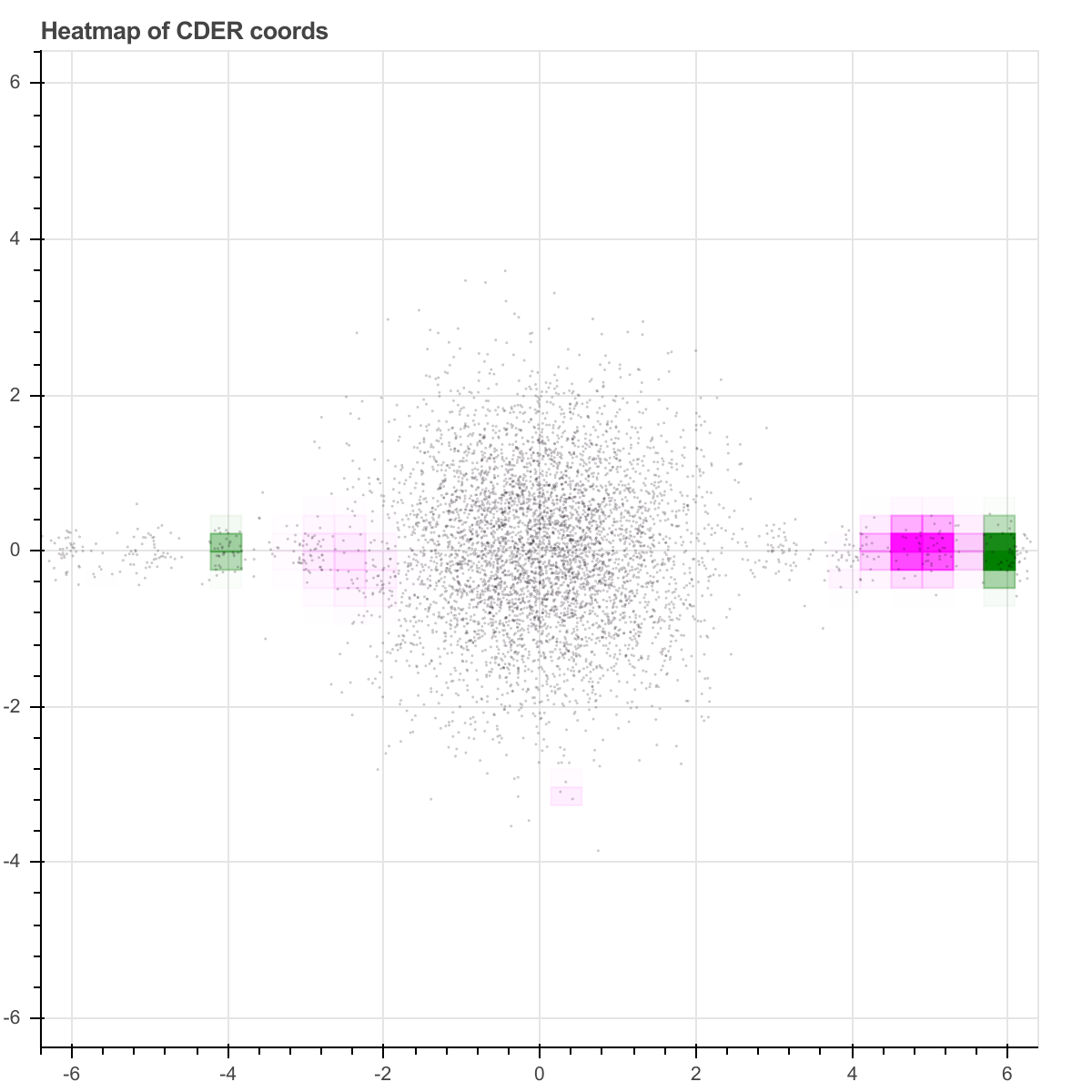
Figure 10. The output of CDER for the example of Figure 2. Regions are shaded by certainty (1-entropy).

In a typical run, the algorithm terminates at cover-tree level 8, even though the complete cover tree of $\underline{\mathcal{X}}$ ends at level 14. A total of 26 distributional coordinates are produced, and their weights vary by about 3 orders of magnitude. Table 1 shows how conservative the entropy-reduction process is at selecting regions to generate distributional coordinates.

$\ell$	$|A_{\ell}|$	$|\hat{A}_{\ell}|$	new Gaussians
0	1	1	+0
1	7	7	+0
2	29	29	+4
3	119	37	+7
4	446	36	+7
5	1379	40	+6
6	2827	23	+1
7	3903	3	+1

Table 1. CDER is parsimonious about selecting cover-tree regions for distributional coordinates.

To judge accuracy on testing data in a supervised-learning scenario, we need a method to label a test pointcloud using the distributional coordinates. Each test pointcloud $X_{\mathrm{test}}$ is mapped to a point in $\mathbb{R}^{26}$. Many sophisticated methods are possible, but for simplicity, we simply ask: For a given pointcloud $X_{\mathrm{test}}$, which is bigger: the Euclidean norm of the magenta Gaussian coordinates evaluated on $X_{\mathrm{test}}$,

$$\sqrt{\sum_{g~{}\mathrm{magenta}}\left(\int_{X_{\mathrm{test}}}g\right)^{2}}$$

or the Euclidean norm of the green Gaussian coordinates evaluated on $X_{\mathrm{test}}$,

$$\sqrt{\sum_{g~{}\mathrm{green}}\left(\int_{X_{\mathrm{test}}}g\right)^{2}}?$$

With this simple comparison, the algorithm achieves 100% accuracy in a 5-fold cross-validation of this cloud collection with a 80/20 training/testing split. More precisely, for each run of the cross-validation, we take 80 percent of the point clouds, turn these into a cloud collection, build distributional coordinates using this cloud collection, and then test the results on the remaining 20 percent of the point clouds. This entire procedure is then repeated five times.

Moreover, the relative masses of the 28 distributional coordinates vary over four orders of magnitude, so for this sort of comparison, one could dispose of many of them in the interest of speed while preserving accuracy. Note that these distributions are contrived to have the same mass (0-moment) and mean (1-moment) and variance. Elementary statistical tests would not distinguish them; 2-moments or skewness tests would be necessary.

7.2. Blocks

This example shows that CDER is fairly robust against background noise that prevents strict separation. It also demonstrates that smoothness of the underlying distributions is not necessary for good results.

Consider two labels: 0/magenta and 1/green. The cloud collection consists of 100 magenta pointclouds and 100 green pointclouds. Each magenta pointcloud in generated by sampling 30 points uniformly in the unit square, as well as 2 extra points sampled uniformly in a $0.1\times 0.1$ square at $(\frac{1}{4},\frac{1}{4})$, as well as 2 extra points sampled uniformly in a $0.1\times 0.1$ square at $(\frac{1}{2},\frac{1}{2})$. Each green pointcloud in generated by sampling 30 points uniformly in the unit square, as well as 2 extra points sampled uniformly in a $0.1\times 0.1$ square at $(\frac{3}{4},\frac{3}{4})$, as well as 2 extra points sampled uniformly in a $0.1\times 0.1$ square at $(\frac{1}{2},\frac{1}{2})$. See Figures 1 and 11.

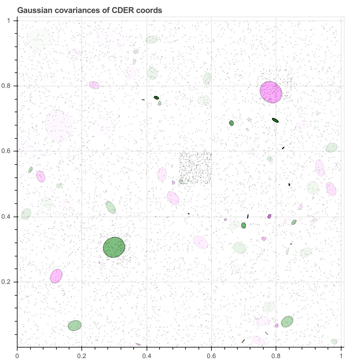
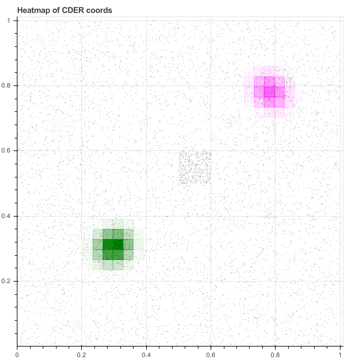
Figure 11. The distributional coordinates found by CDER from Figure 1.

.

Using the same simple comparison as in Section 7.1, the algorithm achieves 88% accuracy despite the high background noise.

7.3. Deep Field

In this example, we demonstrate that Gaussian mixtures are (nearly) “fixed points” of CDER. It also demonstrates that the algorithm can handle unequal sample sizes via the weighting system in Section 2.

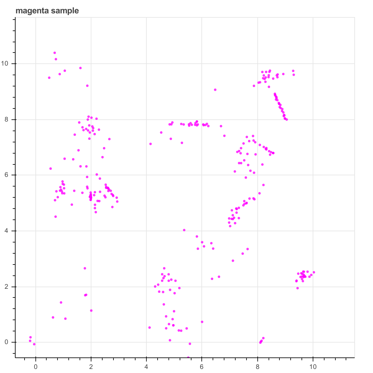
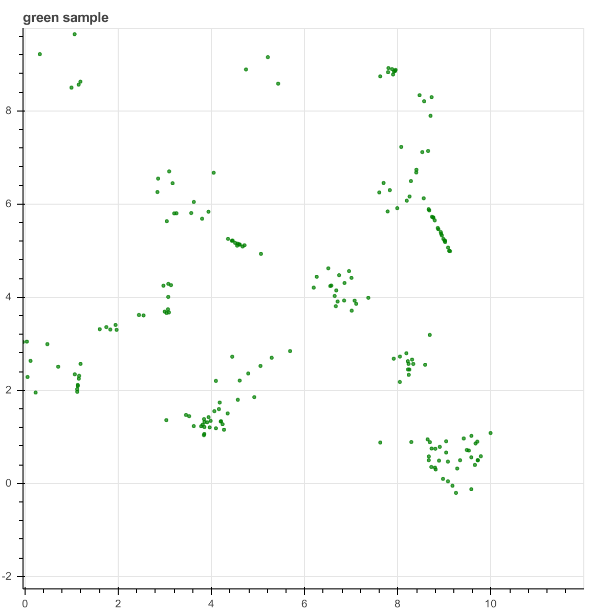
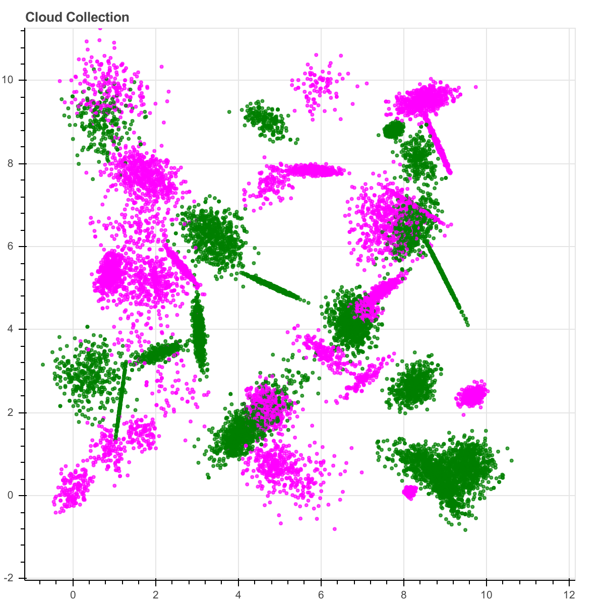
Figure 12. A single magenta pointcloud, a single green pointcloud, and the total cloud collection for a random “deep field” example.

Consider two labels: 0/magenta and 1/green. The underlying distribution is build from 50 Gaussian distributions. For each of these, we choose a random label. We choose a mean point, uniformly on the $10\times 10$ square. We choose a pair of orthonormal covariances uniformly from $0$ to $0.5$. We choose a random rotation angle. We choose an amplification factor (that is, a sample size) uniformly between 50 and 5000. For a particular random seed, we arrive at some combined density function $f_{0}$ and $f_{1}$, as in Figure 14

Then, for each label, we produce between 20 and 40 pointclouds, each with between 50 and 500 points. For a particular random seed, we arrive at the cloud collection in Figure 12.

The CDER algorithm builds a Gaussian mixture model focused on regions of low entropy (Figure 13), so it should not be surprising that it builds Gaussians near the original Gaussians, as in Figure 14.

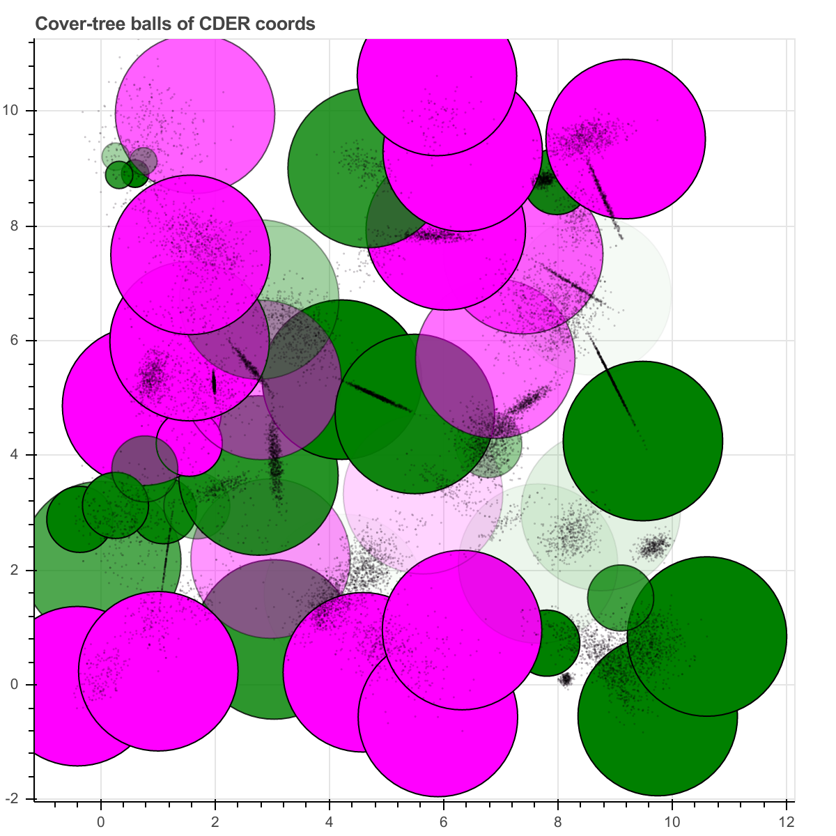
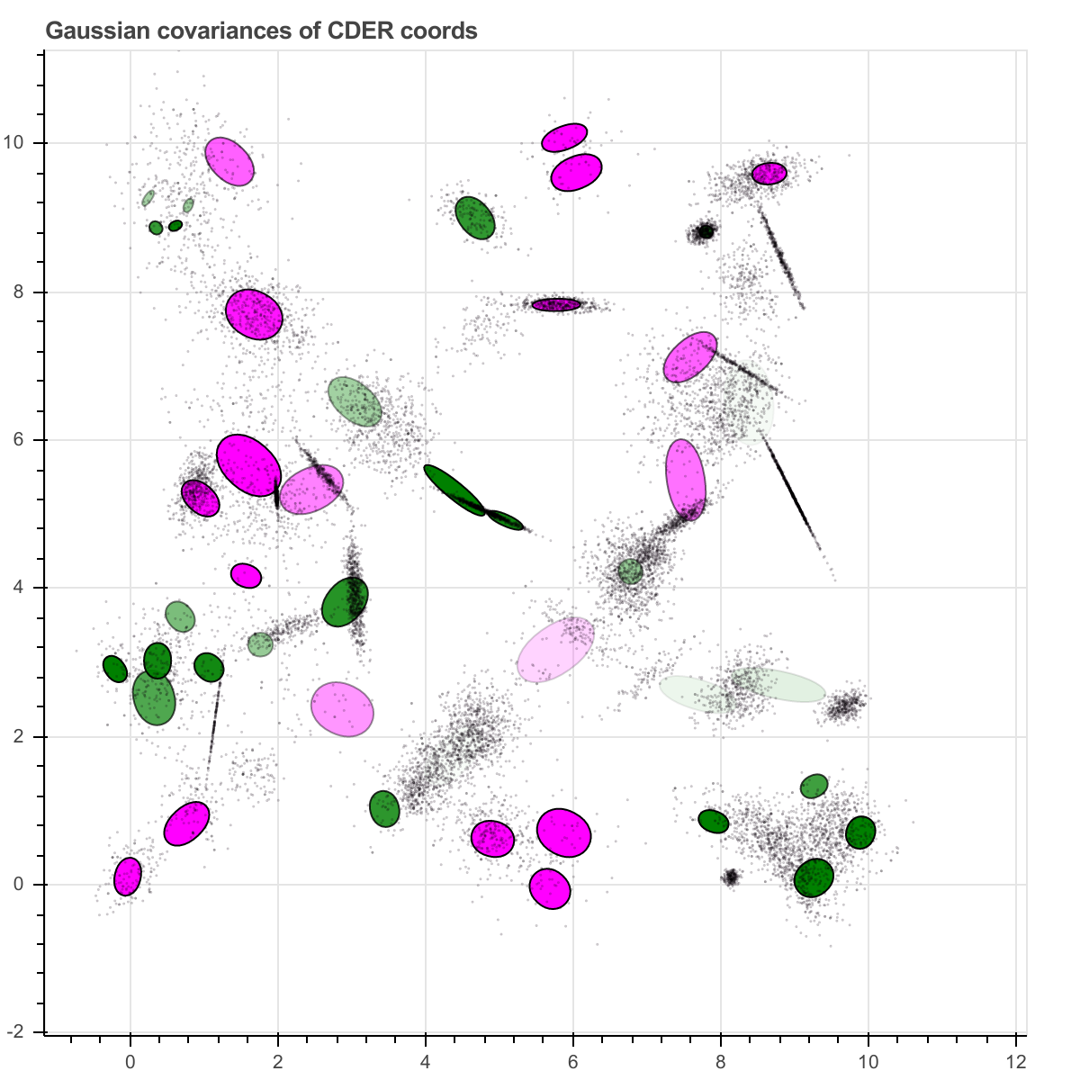
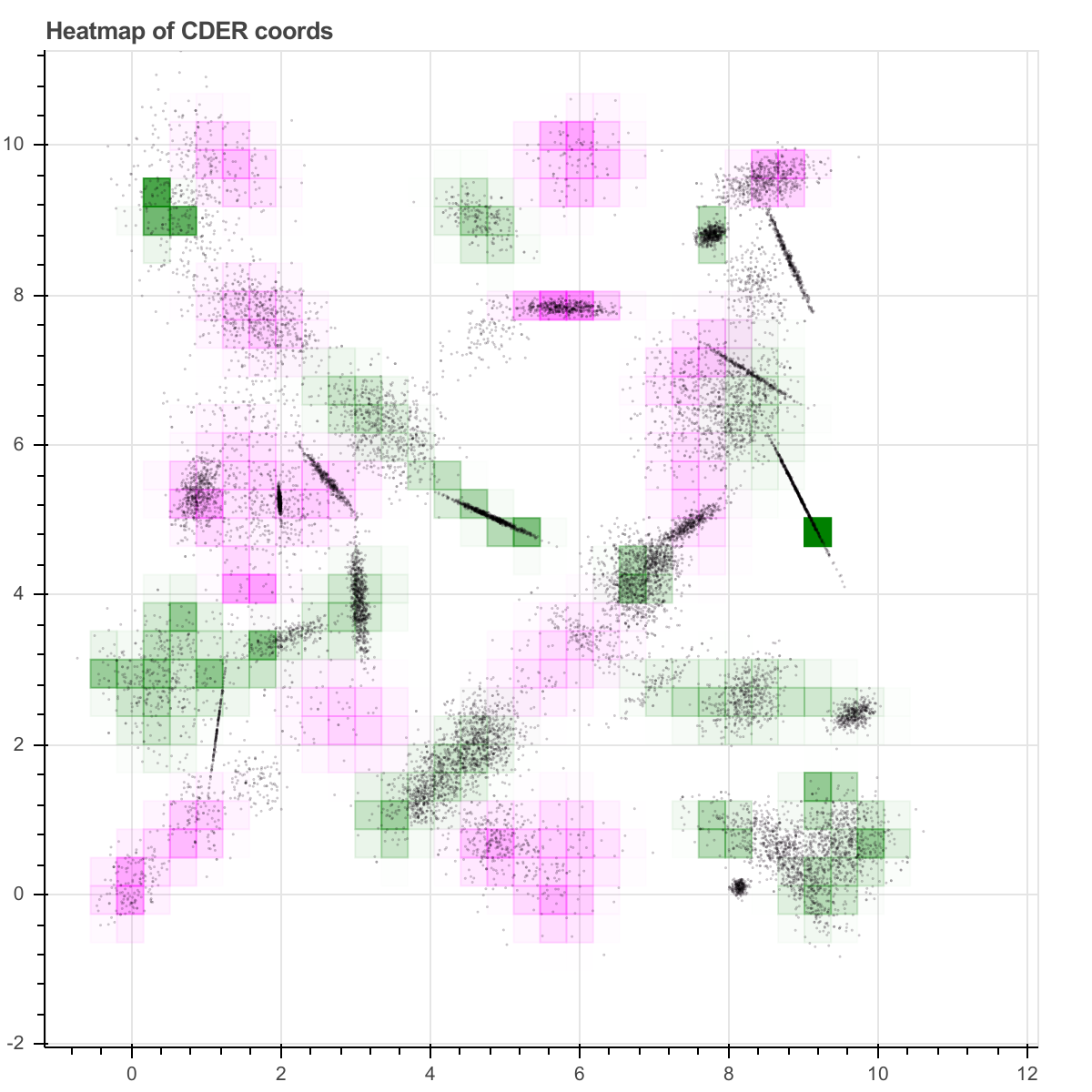
Figure 13. The regions and distributional coordinates detected by CDER in the “deep field” example.

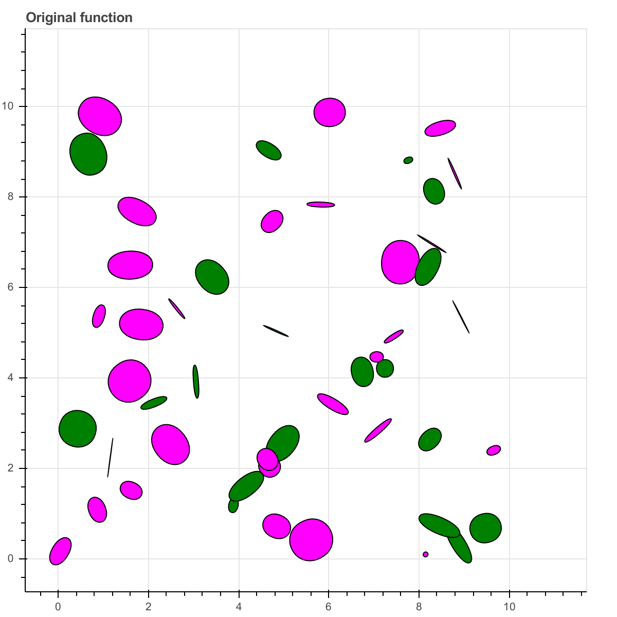
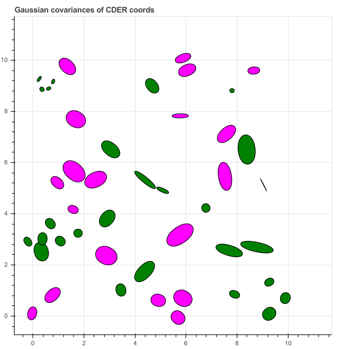
Figure 14. Left: The original randomly-generated Gaussian mixture model. Right: The Gaussian mixture model returned by CDER.

7.4. Three Labels

For simplicity, the previous examples have involved only two labels. In a two-label system, a low-entropy region has exactly one dominant label. However, the algorithm is sensible for any number of labels, and it may be that the low-entropy regions are dominated by multiple labels. Hence, an ensemble of regions may be necessary to distinguish pointclouds.

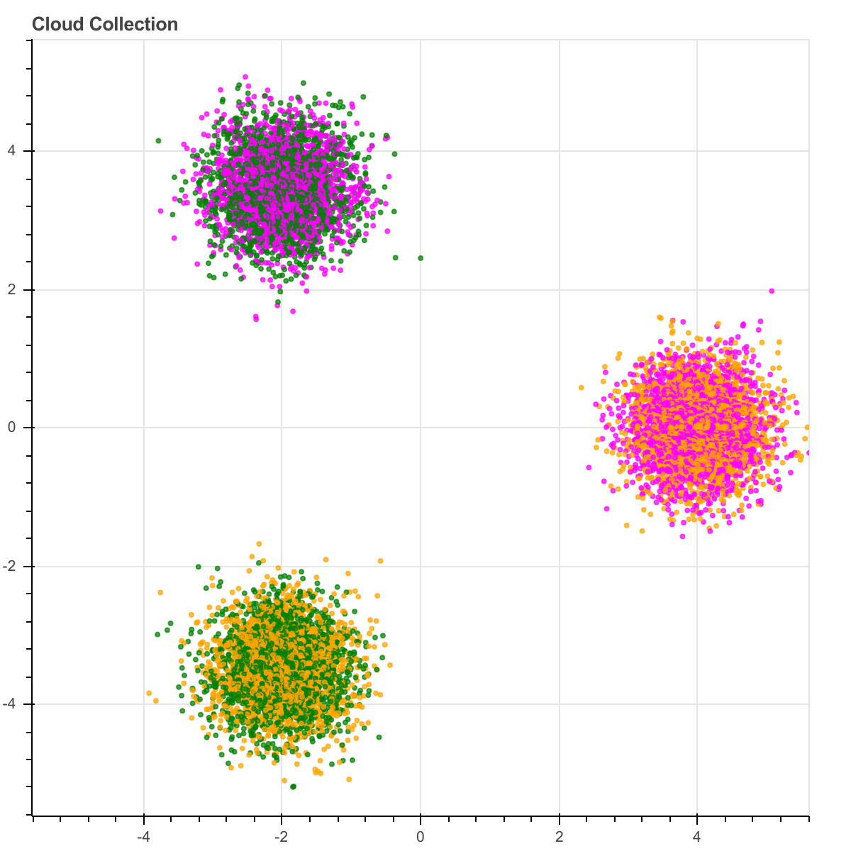
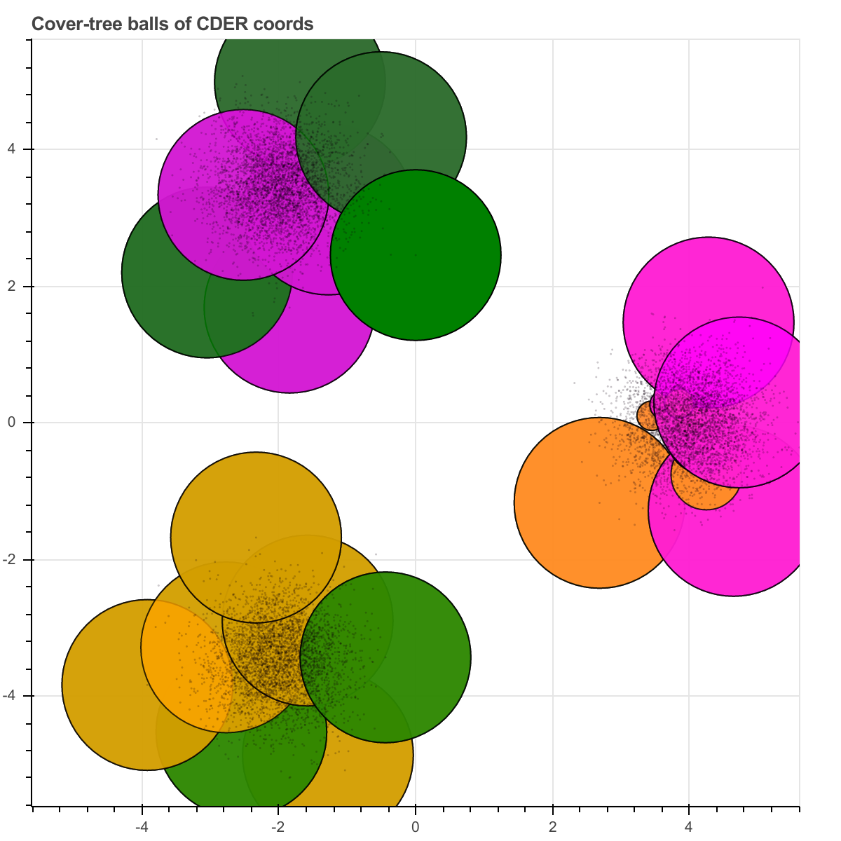
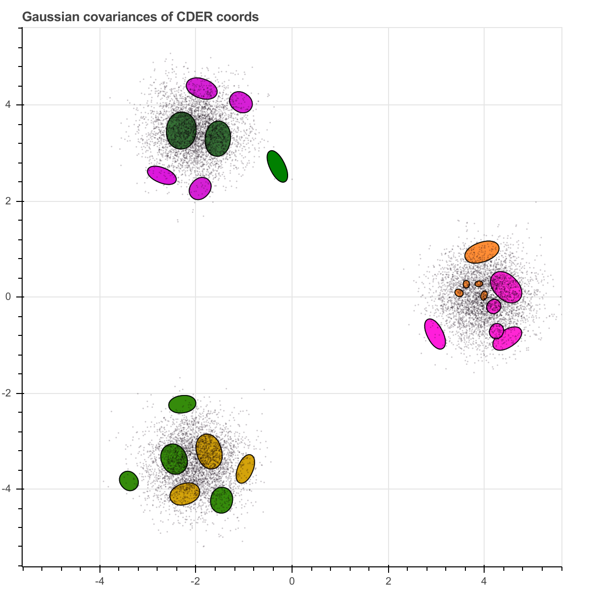
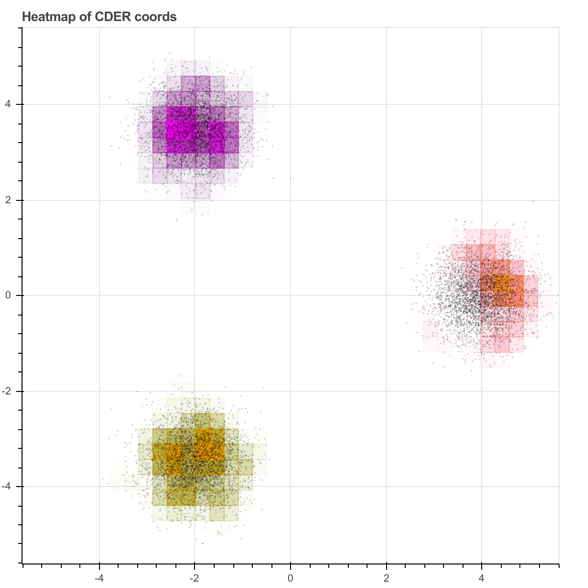
Figure 15. A three-label task without unique dominance. Upper-left: the original cloud collection. Upper-right: The cover-tree balls used by CDER. Lower-left: The Gaussian covariances constructed by CDER. Lower-right: Heatmap of resulting distributional coordinates.

Consider three labels: 0/magenta, 1/green, and 2/orange. Let $f_{0}$ be a triple of standard normal distributions: one each at $(0,0)$, $(4,0)$, and $(-2,2\sqrt{3})$. Let $f_{1}$ be a triple of standard normal distributions: one each at $(0,0)$,$(-2,2\sqrt{3})$, and $(-2,-2\sqrt{3})$. $(-2,2\sqrt{3})$, and $(-2,-2\sqrt{3})$. Let $f_{2}$ be a triple of standard normal distributions: one each at $(0,0)$, $(-2,-2\sqrt{3})$, and $(4,0)$. See Figure 15.

The CDER algorithm detects these shared regions perfectly, achieving 100% in a 5-fold cross-validation of this cloud collection with a 80/20 training/testing split, using the same simple comparison method as in Section 7.1.

8. Stability

Ideally, one would like to prove that CDER is stable or backward-stable, in the sense of [14, Lecture 14]. To formulate stability or backward-stability, CDER must be expressed as a numerical approximation of a formal function between normed vector spaces.

Let $C$ denote the vector space of piecewise continuous functions on our compact domain. Define a norm on $C\times C$ by $\|(f_{1},f_{2})\|=\sqrt{\|f_{1}\|_{2}^{2}+\|f_{2}\|_{2}^{2}}$, where each term is the $L_{2}$ norm on our (compact) domain. Given two “input ”functions $(f_{1},f_{2})\in V$ we consider them as density functions for each of two labels. Consider the pointwise entropy,

$$H(x)=-\frac{f_{1}(x)}{f_{1}(x)+f_{2}(x)}\log_{2}\left(\frac{f_{1}(x)}{f_{1}(x)+f_{2}(x)}\right)-\frac{f_{2}(x)}{f_{1}(x)+f_{2}(x)}\log_{2}\left(\frac{f_{2}(x)}{f_{1}(x)+f_{2}(x)}\right).$$

Let $T$ denote the formal function $T:C\times C\to C\times C$ by $T(f_{1},f_{2})=(g_{1},g_{2})$ where

(4) $$g_{1}(x)=\begin{cases}H(x)f_{1}(x),&\text{if $f_{1}(x)>f_{2}(x)$,}\\ 0,&\text{otherwise}.\end{cases}$$

and

(5) $$g_{2}(x)=\begin{cases}H(x)f_{2}(x),&\text{if $f_{2}(x)>f_{1}(x)$,}\\ 0,&\text{otherwise}.\end{cases}$$

A numerical algorithm $\tilde{T}$ for $T$ can be obtained roughly as “sample equally from $f_{1}$ and $f_{2}$, and apply CDER to generate weighted distributional coordinates. The weighted sum of the distributional coordinates for label 1 is $g_{1}$, and the sum of the distributional coordinates for label 2 is $g_{2}$.” A stability result such as this is a subject of future work. We have not yet succeeded in proving either stability statement for CDER, but the high cross-validation of the examples above is promising.

9. Discussion

This paper introduced CDER, a data-driven, label-driven feature extraction method for collections of labeled pointclouds. CDER is fast, both in terms of theoretical complexity and in initial tests on examples. It does not require the user to choose any tuning parameters, and the geometric meaning of its output features are transparently clear. This section outlines some future directions and makes a few generalizing remarks.

The attentive reader of Section 4 may notice that cover trees can be defined in an arbitrary metric space, and indeed this is how they were originally defined [7]. We use them to construct distributional coordinates, and our algorithm for doing so (Section 6) demands that we be able to quickly compute means of sets of points. While the Fréchet Mean ([5], IX) can be defined in any metric space, there are not always fast algorithms for its computation (it also need not exist in all cases). And so while more generality could be achieved in the definition of CDER, we only make our complexity statements for cloud collections in a common Euclidean space.

All examples in Section 7 were artificial, and simply intended to help visualize the novel and fairly-technical CDER algorithm and emphasize its key properties. Future work will involve applications of CDER to real data from a variety of real fields, including large administrative datasets of interest to social scientists and to vehicle tracking [4].

We also hope that CDER will prove useful as a feature-extraction method in topological data analysis [6], since persistence diagrams can be thought of as point clouds in the plane. Future work will compare the performance of CDER against other such feature-extraction methods (for example, [12] and [1]).

Finally, we recall the weighting discussion in Section 2, where we used the simplifying assumptions that each color/label was equally likely and that each point within a single point cloud should be given equal weight. We note that CDER can be easily adapted to accommodate other prior assumptions about relative likelihoods of labels or even prior assumptions about outlier status of certain points in a cloud, say as part of a Bayesian learning process.

References

- [1] A. Adcock, E. Carlsson, and G. Carlsson. The ring of algebraic functions on persistence bar codes. ArXiv e-prints, 2013.
- [2] William K. Allard, Guangliang Chen, and Mauro Maggioni. Multi-scale geometric methods for data sets ii: Geometric multi-resolution analysis. Applied and Computational Harmonic Analysis, 32(3):435 – 462, 2012.
- [3] John C. Baez, Tobias Fritz, and Tom Leinsterm. A characterization of entropy in terms of information loss. Entropy, 13(11):1945–1957, 2011.
- [4] Paul Bendich, Sang Chin, Jesse Clarke, John deSena, John Harer, Elizabeth Munch, Andrew Newman, David Porter, David Rouse, Nate Strawn, and Adam Watkins. Topological and statistical behavior classifiers for tracking applications. IEEE Trans. on Aero. and Elec. Sys., 52(6):2644–2661, 2016.
- [5] D. Burago, I.U.D. Burago, and S. Ivanov. A Course in Metric Geometry. Crm Proceedings & Lecture Notes. American Mathematical Society, 2001.
- [6] Herbert Edelsbrunner and John Harer. Persistent Homology — a Survey. Contemporary Mathematics, 0000:1–26.
- [7] Sariel Har-Peled and Manor Mendel. Fast construction of nets in low-dimensional metrics and their applications. SIAM Journal on Computing, 35(5):1148–1184.
- [8] Trevor Hastie, Robert Tibshirani, and Jerome Friedman. The Elements of Statistical Learning. Springer Series in Statistics. Springer New York Inc., New York, NY, USA, 2001.
- [9] Michael Kerber, Dmitriy Morozov, and Arnur Nigmetov. Geometry Helps to Compare Persistence Diagrams, pages 103–112. 2016.
- [10] S. Kullback and R. A. Leibler. On information and sufficiency. Ann. Math. Statist., 22(1):79–86, 03 1951.
- [11] James R. Munkres. Elements of Algebraic Topology. Addison Wesley, 1993.
- [12] Jan Reininghaus, Stefan Huber, Ulrich Bauer, and Roland Kwitt. A stable multi-scale kernel for topological machine learning. In Proceedings of the IEEE Conference on Computer Vision and Pattern Recognition, pages 4741–4748, 2015.
- [13] Donald R. Sheehy. Linear-size approximations to the Vietoris-Rips filtration. Discrete & Computational Geometry, 49(4):778–796, 2013.
- [14] Lloyd N. Trefethen and D Bau III. Numerical linear algebra. Numerical Linear Algebra with Applications, 12:361, 1997.