Rician MIMO Channel- and Jamming-Aware Decision Fusion

Abstract

In this manuscript we study channel-aware decision fusion (DF) in a wireless sensor network (WSN) where: ($i$) the sensors transmit their decisions simultaneously for spectral efficiency purposes and the DF center (DFC) is equipped with multiple antennas; ($ii$) each sensor-DFC channel is described via a Rician model. As opposed to the existing literature, in order to account for stringent energy constraints in the WSN, only statistical channel information is assumed for the non-line-of-sight (scattered) fading terms. For such a scenario, sub-optimal fusion rules are developed in order to deal with the exponential complexity of the likelihood ratio test (LRT) and impractical (complete) system knowledge. Furthermore, the considered model is extended to the case of (partially unknown) jamming-originated interference. Then the obtained fusion rules are modified with the use of composite hypothesis testing framework and generalized LRT. Coincidence and statistical equivalence among them are also investigated under some relevant simplified scenarios. Numerical results compare the proposed rules and highlight their jamming-suppression capability.

I Introduction

I-A Motivation and Related Literature

Decision Fusion (DF) in a wireless sensor network (WSN) consists in transmitting local decisions about an observed phenomenon from sensors to a DF center (DFC) for a global decision, with the intent of surveillance and/or anomaly detection [1]. Typically all the studies had been focused on a parallel access channels (PACs) with instantaneous [2, 3] or statistical channel-state information (CSI) [4], although some recent works extended to the case of multiple access channels (MACs). Adoption of a MAC in WSNs is clearly attractive because of its increased spectral efficiency.

Distributed detection over MACs was first studied in [5], where perfect compensation of the fading coefficients is assumed for each sensor. Non-coherent modulation and censoring over PACs and MACs were analyzed in [6] with emphasis on processing gain and combining loss. The same scenario was studied in [7], focusing on the error exponents (obtained through the large deviation principle) and the design of energy-efficient modulations for Rayleigh and Rice fading. Optimality of received-energy statistic in Rayleigh fading scenario was demonstrated for diversity MACs with non-identical sensors in [8]. Efficient DF over MACs only with knowledge of the instantaneous channel gains and with the help of power-control and phase-shifting techniques was studied in [9]. Techniques borrowed from direct-sequence spread-spectrum systems were combined with on-off keying (OOK) modulation and censoring for DF in scenarios with statistical CSI [10].

DF over a (virtual) MIMO (this setup will be referred to as “MIMO-DF” hereinafter) was first proposed in [11], with focus on power-allocation design based on instantaneous CSI, under the framework of J-divergence. Distributed detection with ultra-wideband sensors over MAC was then studied in [12]. The same model was adopted to study sensor fusion over MIMO channels with amplify-and-forward sensors in [13, 14]. A recent theoretical study on data fusion with amplify and forward sensors, Rayleigh fading channel and a large-array at the DFC has been presented in [15].

Design of several sub-optimal fusion rules for MIMO-DF scenario was given in [16] in a setup with instantaneous CSI and Rayleigh fading, while the analysis was extended in [17] to a large-array at the DFC, estimated CSI and inhomogeneous large scale fading. In both cases binary-phase shift keying (BPSK) has been employed. It is worth noticing that in MIMO-DF scenario the log-likelihood ratio (LLR) is not a viable solution, since it suffers from the exponential growth of the computational complexity with respect to (w.r.t.) the number of sensors and a strong requirement on system knowledge.

However, frequently the final purpose of a WSN is anomaly detection (viz. the null hypothesis is much more frequent than the alternative hypothesis, denoting the “anomaly”). Such problem arises in many application contexts, such as intrusion detection or monitoring of hazardous events. In this case, a wise choice of the modulation format is the on-off keying (OOK), which ensures a nearly-optimal censoring policy (and thus significant energy savings) [6, 18]. Additionally, though the channel between the sensors and the DFC may be accurately modelled as Rician, assuming instantaneous CSI (i.e., estimation of the scattered fading component) may be too energy costly for an anomaly detection problem. This motivated the study of DF over Rician MAC channels (in the single-antenna DFC case) with only statistical CSI in [7, 19]. We point out that statistical CSI is instead a reasonable assumption for a WSN and can be obtained through long-term training-based techniques (since statistical parameters of Rician model have a slower variation with respect to the coherence time of the channel), mimicking the procedures proposed in [20]. The aforementioned problem may be further exacerbated by the presence of a (possibly distributed) jamming device in the WSN deployment area [21]. Such problem is clearly relevant in non-friendly environments, such as the battlefield, where malicious devices (i.e., the jammers) are placed to hinder the operational requirements of the WSN. Indeed, due to jammer hostile nature, unknown interference is superimposed to useful received signal (containing “informative” sensors contributions). Therefore, additional relevant parameters may be unknown at the DFC side. This precludes development of sub-optimal (simplified) fusion rules based on the LLR, which assume complete specification of pdfs under both hypotheses. To the best of our knowledge, the study of such a setup for MIMO-DF has not been addressed yet in the open literature.

I-B Main Results and Paper Organization

The contributions of the present manuscript are summarized as follows.

• We study decision fusion over MAC with Rician fading and multiple antennas at the DFC (as opposed to [7, 19]). In the present study only the LOS component is assumed known at the DFC. Also, by adopting the same general assumptions in [17], the considered model also accounts for unequal long-term received powers from the sensors, through a common path loss and shadowing model;

• We derive sub-optimal fusion rules dealing with exponential complexity and with required system knowledge in the considered scenario, namely, we derive ($i$) “ideal sensors” (IS) (following the same spirit as in [2, 22]), ($ii$) “non-line of sight” (NLOS), ($iii$) “widely-linear” (mimicking [17]) and ($iv$) “improper Gaussian moment matching” (IGMM, based on second order characterization of the received vector under both hypotheses) rules;

• Subsequently, we consider DF in the presence of a (either distributed or co-located) multi-antenna jamming device, whose communication channel is described by an analogous Rician model. The problem is tackled within a composite hypothesis testing framework and solved via the generalized likelihood-ratio test (GLRT) [23] and similar key simplifying assumptions as in the “no-jamming” scenario, thus leading to IS-GLRT, NLOS-GLRT and IGMM-GLRT rules, respectively;

• Simulation studies (along with a detailed complexity analysis) are performed to compare the performance of the considered rules and verify the asymptotical equivalences (later proved in Secs. III-F and IV-E) among them in some specific instances. Also, the performance trend as a function of the Rician parameters of the WSN and the jammer, the thermal noise and the number of receive antennas are investigated and discussed.

The remainder of the manuscript is organized as follows: Sec. II introduces the model; in Sec. III we derive and study the fusion rules, while in Sec. IV we generalize the analysis to the case of a subspace interference; the obtained rules are compared in terms of computational complexity in Sec. V; in Sec. VI we compare the presented rules through simulations; finally in Sec. VII we draw some conclusions; proofs and derivations are contained in a dedicated Appendix.

Notation - Lower-case (resp. Upper-case) bold letters denote vectors (resp. matrices), with $a_{n}$ (resp. $a_{n,m}$) being the $n$th (resp. the $(n,m)$th) element of $\bm{a}$ (resp. $\bm{A}$); upper-case calligraphic letters denote finite sets, with $\mathcal{A}^{K}$ representing the $k$-ary Cartesian power of $\mathcal{A}$; $\bm{O}_{N\times K}$ (resp. $\bm{I}_{N}$) denotes the $N\times K$ (resp. $N\times N$) null (resp. identity) matrix, with corresponding short-hand notation $\bm{O}_{N}$ for a square matrix; $\bm{0}_{N}$ (resp. $\bm{1}_{N}$) denotes the null (resp. ones) vector of length $N$; $\bm{a}_{n:m}$ (resp. $\bm{A}_{n:m}$) denotes the sub-vector of $\bm{a}$ (resp. the sub-matrix of $\bm{A}$) obtained from selecting only $n$th to $m$th elements of $\bm{v}$ (resp. $n$th to $m$th rows/columns of $\bm{A}$); $\mathbb{E}\{\cdot\}$, $\mathrm{var\{\cdot\}}$, $(\cdot)^{T}$, $(\cdot)^{\dagger}$, $(\cdot)^{-}$, $\Re\left(\cdot\right)$, $\Im(\cdot)$ and $\left\|\cdot\right\|$ denote expectation, variance, transpose, conjugate transpose, pseudo-inverse, real part, imaginary part and Euclidean norm operators, respectively; $(\cdot)_{+}$ is used to indicate $\max\{0,\cdot\}$; $\mathrm{diag}(\bm{A})$ (resp. $\mathrm{diag}(\bm{a})$) denotes the diagonal matrix extracted from $\bm{A}$ (resp. the diagonal matrix with main diagonal given by $\bm{a}$); $\mathrm{det(}\bm{A})$ is used to denote the determinant of $\bm{A}$; $\mathrm{\lambda{}_{min}}(\bm{A})$ denotes the minimum eigenvalue of the Hermitian matrix $\bm{A}$; $\bm{P}_{\bm{X}}^{\perp}$ denotes the orthogonal projector to the range space spanned by $\bm{X}$; $\underline{\bm{a}}$ (resp. $\underline{\bm{A}}$) denotes the augmented vector (resp. matrix) of $\bm{a}$ (resp. $\bm{A}$), that is $\underline{\bm{a}}\triangleq\left[\begin{array}[]{cc}\bm{a}^{T}&\bm{a}^{\dagger}\end{array}\right]^{T}$ (resp. $\underline{\bm{A}}\triangleq\left[\begin{array}[]{cc}\bm{A}^{T}&\bm{A}^{\dagger}\end{array}\right]^{T}$); $P(\cdot)$ and $p(\cdot)$ denote probability mass functions (pmf) and probability density functions (pdf), while $P(\cdot|\cdot)$ and $p(\cdot|\cdot)$ their corresponding conditional counterparts; $\bm{\Sigma}_{\bm{x}}$ (resp. $\bar{\bm{\Sigma}}_{\bm{x}}$) denotes the covariance (resp. the complementary covariance) matrix of the complex-valued random vector $\bm{x}$; $\mathcal{N}_{\mathbb{C}}(\bm{\mu},\bm{\Sigma})$ (resp. $\mathcal{N}_{\mathbb{C}}(\bm{\mu},\bm{\Sigma},\bar{\bm{\Sigma}}$) denotes a proper (resp. an improper) complex normal distribution with mean vector $\bm{\mu}$ and covariance matrix $\bm{\Sigma}$ (resp. covariance $\bm{\Sigma}$ and pseudo-covariance $\bar{\bm{\Sigma}}$), while $\mathcal{N}(\bm{\mu},\bm{\Sigma})$ denotes the corresponding real-valued counterpart; finally the symbols $\propto$, and $\sim$ mean “statistically equivalent to” and “distributed as”, respectively.

II System Model

Hereinafter we will consider a decentralized binary hypothesis test, where $K$ sensors are used to discern between the hypotheses in the set $\mathcal{H}\triangleq\{\mathcal{H}_{0},\mathcal{H}_{1}\}$ (e.g. $\mathcal{H}_{0}/\mathcal{H}_{1}$ may represent the absence/presence of a specific target of interest). The $k$th sensor, $k\in\mathcal{K}\triangleq\{1,2,\ldots,K\}$, takes a binary local decision $\xi_{k}\in\mathcal{H}$ about the observed phenomenon on the basis of its own measurements. Here we do not make any conditional (given $\mathcal{H}_{i}\in\mathcal{H}$) mutual independence assumption on $\xi_{k}$. Each decision $\xi_{k}$ is mapped to a symbol $x_{k}\in{\cal X}=\{0,+1\}$ representing an OOK modulation: without loss of generality (w.l.o.g.) we assume that $\xi_{k}=\mathcal{H}_{i}$ maps into $x_{k}=i$, $i\in\{0,1\}$. The quality of the WSN is characterized by the conditional joint pmfs $P(\bm{x}|\mathcal{H}_{i})$. Also, we denote $P_{D,k}\triangleq P\left(x_{k}=1|\mathcal{H}_{1}\right)$ and $P_{F,k}\triangleq P\left(x_{k}=1|\mathcal{H}_{0}\right)$ the probability of detection and false alarm of the $k$th sensor, respectively (here we make the assumption $P_{D,k}\geq P_{F,k}$, meaning that each sensor decision procedure leads to receive operating characteristics above the chance line [24]). In some situations, aiming at improving clarity of exposition, we will use the short-hand notation $(P_{0,k},P_{1,k})=(P_{F,k},P_{D,k})$ (and $(P_{0},P_{1})=(P_{F},P_{D})$, in the simpler case of conditionally i.i.d. decisions).

Sensors communicate with a DFC equipped with $N$ receive antennas over a wireless flat-fading MAC in order to exploit diversity so as to mitigate small-scale fading; this setup determines a distributed (or virtual) MIMO channel [11, 16]. Also, perfect synchronization, as in [5, 8, 11, 16], is assumed at the DFC.

We denote: $y_{n}$ the signal at the $n$th receive antenna of the DFC after matched filtering and sampling; $(\sqrt{d_{k,k}}\,\bar{h}_{n,k})$ the composite channel coefficient between the $k$th sensor and the $n$th receive antenna of the DFC; $w_{n}$ the additive white Gaussian noise at the $n$th receive antenna of the DFC. The vector model at the DFC is:

$$\bm{y}=\,\, \bar{\bm{H}}\bm{D}^{1/2}\bm{x}+\bm{w}$$ (1)

where $\bm{y}\in\mathbb{C}^{N}$, $\bm{x}\in\mathcal{X}^{K}$ and $\bm{w}\sim\mathcal{N}_{\mathbb{C}}(\bm{0}_{N},\sigma_{w}^{2}\bm{I}_{N})$ are the received-signal vector, the transmitted-signal vector and the noise vector, respectively. Also, the matrices $\bar{\bm{H}}\in\mathbb{C}^{N\times K}$ and $\bm{D}\in\mathbb{C}^{K\times K}$ model independent small-scale fading, geometric attenuation and log-normal shadowing. More specifically, $\bm{D}\triangleq\mathrm{diag}\left(\begin{bmatrix}\beta_{1}&\cdots&\beta_{K}\end{bmatrix}^{T}\right)$ is a (known) matrix with $k$th diagonal element $d_{k,k}=\beta_{k}$ ($\beta_{k}>0$) accounting for path loss and shadow fading experienced by $k$th sensor. On the other hand, the $k$th column of $\bar{\bm{H}}$ models the (small-scale) fading vector of $k$th sensor as $\bar{\bm{h}}_{k}=b_{k}\,\bm{a}(\theta_{k})+\sqrt{1-b_{k}^{2}}\,\bm{h}_{k}$. Here $\bm{a}(\cdot)$ denotes the steering vector (which depends on the angle-of-arrival $\theta_{k}$, assumed known at the DFC) corresponding to the LOS component and $\bm{h}_{k}\sim\mathcal{N}_{\mathbb{C}}(\bm{0}_{N},\bm{I}_{N})$ corresponds to the normalized NLOS (scattered) component. Finally, we denote $b_{k}\triangleq\sqrt{\frac{\kappa_{k}}{1+\kappa_{k}}}$, where $\kappa_{k}$ represents the (known) usual Rician factor between $k$th sensor and DFC.

The matrix $\bar{\bm{H}}$ can be expressed compactly in terms of the relevant matrices $\bm{A}(\bm{\theta})\triangleq\begin{bmatrix}\bm{a}(\theta_{1})&\cdots&\bm{a}(\theta_{K})\end{bmatrix}$, $\bm{H}\triangleq\begin{bmatrix}\bm{h}_{1}&\cdots&\bm{h}_{K}\end{bmatrix}$ and $\bm{R}\triangleq\mathrm{diag}\left(\begin{bmatrix}b_{1}&\cdots&b_{K}\end{bmatrix}^{T}\right)$, respectively, as

$$\bar{\bm{H}}\triangleq\,\,\bm{A}(\bm{\theta})\,\bm{R}+\bm{H}\,(\bm{I}_{K}-\bm{R}^{2})^{1/2}\,.$$ (2)

Finally, we underline that the received scattered term from $k$th sensor in Eq. (1) is $\sqrt{(1-b_{k}^{2})\,\beta_{k}}\,\bm{h}_{k}\sim\mathcal{N}_{\mathbb{C}}(\bm{0}_{N},\nu_{k}\,\bm{I}_{N})$, where $\nu_{k}\triangleq[\beta_{k}\,(1-b_{k}^{2})]$, while its LOS term is $\bm{\mu}_{k}\triangleq[\sqrt{\beta_{k}}\,b_{k}\,\bm{a}(\theta_{k})]$ and corresponds to the $k$th column of the matrix

$$\widetilde{\bm{A}}(\bm{\theta})\triangleq\left(\bm{A}(\bm{\theta})\,\bm{R}\,\bm{D}^{1/2}\right)\,,$$ (3)

denoting the matrix of received LOS terms from the WSN.

III Fusion Rules

III-A Optimum (LLR) Rule

The optimal test [23] is formulated on the basis of the LLR $\Lambda_{\mathrm{opt}}\triangleq\ln\left[\frac{p(\bm{y}|\mathcal{H}_{1})}{p(\bm{y}|\mathcal{H}_{0})}\right]$, and decides in favour of $\mathcal{H}_{1}$ (resp. $\mathcal{H}_{0}$) when $\Lambda_{\mathrm{opt}}>\gamma$ (resp. $\Lambda_{\mathrm{opt}}\leq\gamma$), with $\gamma$ denoting the threshold which the LLR is compared to. After few manipulations, the LLR can be expressed explicitly as

$$\Lambda_{\mathrm{opt}}=\ln\left[\frac{\sum_{\bm{x}\in\mathcal{X}^{K}}\frac{P(\bm{x}|\mathcal{H}_{1})}{[\sigma_{e}^{2}(\bm{x})]^{N}}\exp(-\frac{\bm{\|y}-\sum_{k=1}^{K}\bm{\mu}_{k}\,x_{k}\|^{2}}{\sigma_{e}^{2}(\bm{x})})}{\sum_{\bm{x}\in\mathcal{X}^{K}}\frac{P(\bm{x}|\mathcal{H}_{0})}{[\sigma_{e}^{2}(\bm{x})]^{N}}\exp(-\frac{\bm{\|y}-\sum_{k=1}^{K}\bm{\mu}_{k}\,x_{k}\|^{2}}{\sigma_{e}^{2}(\bm{x})})}\right]$$ (4)

where $\sigma_{e}^{2}(\bm{x})\triangleq(\sigma_{w}^{2}+\sum_{k=1}^{K}\nu_{k}\,x_{k})$. The above result follows from $\bm{y}|\mathcal{H}_{i}$ being a Gaussian mixture random vector, since the pdf under each hypothesis can be obtained as $p(\bm{y}|\mathcal{H}_{i})=\sum_{\bm{x}}p(\bm{y}|\bm{x})\,P(\bm{x}|\mathcal{H}_{i})$ (the directed triple $\mathcal{H}\rightarrow\bm{x}\rightarrow\bm{y}$ satisfies the Markov property). It is apparent that implementation of Eq. (4) requires a computational complexity which grows exponentially with $K$ (namely $\mathcal{O}(2^{K})$, where $\mathcal{O}(\cdot)$ stands for the usual Landau’s notation). Also, differently from [16, 17] (where a BPSK modulation is employed), the computation here is complicated by the fact that each component of the mixture (under $\mathcal{H}_{i}$) has both different mean vectors and covariance (actually scaled identity) matrices. Therefore, sub-optimal fusion rules with reduced complexity are investigated in what follows.

III-B Ideal sensors (IS) rule

The LLR in Eq. (4) can be simplified under the assumption of perfect sensors [3, 16, 25], i.e., $P(\bm{x}=\bm{1}_{K}|\mathcal{H}_{1})=P(\bm{x}=\bm{0}_{K}|\mathcal{H}_{0})=1$. In this case $\bm{x}\in\{\bm{0}_{K},\bm{1}_{K}\}$ and Eq. (4) reduces to [16]:

$$\ln\left[\frac{[\sigma_{e}^{2}(\bm{1}_{K})]^{-N}\,\exp\left(-\frac{\bm{\|y}-\sum_{k=1}^{K}\bm{\mu}_{k}\|^{2}}{\sigma_{e}^{2}(\bm{1}_{K})}\right)}{[\sigma_{w}^{2}]^{-N}\,\exp\left(-\frac{\bm{\|y}\|^{2}}{\sigma_{w}^{2}}\right)}\right]\propto$$

$$2\,\Re(\bar{\bm{\mu}}^{\dagger}\bm{y})+\frac{\bar{\nu}}{\sigma_{w}^{2}}\left\|\bm{y}\right\|^{2}\triangleq\Lambda_{{\scriptscriptstyle\mathrm{IS}}}$$ (5)

where $\bar{\bm{\mu}}\triangleq\frac{1}{K}\sum_{k=1}^{K}\bm{\mu}_{k}$ and $\bar{\nu}\triangleq\frac{1}{K}\sum_{k=1}^{K}\nu_{k}$ and terms independent from $\bm{y}$ have been discarded (as they can be incorporated in a suitably modified threshold $\gamma$).

It is worth noticing that the assumption of perfect local decisions is used only for system design purposes, and does not mean that the system is working under such ideal conditions, thus the rule is suboptimal. Also, we observe that IS rule in (5) is formed by a weighted combination of a maximum ratio combiner (MRC, which actually is the statistic resulting from IS assumption on the known part of channel vector at the DFC [16]) and an energy detector (ED, i.e., the statistic arising from the IS assumption on the random part of the channel vector at the DFC [8]). Clearly, from Eq. (5) it is apparent that IS rule does not require sensor performance (i.e., the pmf $P(\bm{x}|\mathcal{H}_{i})$, $i\in 0,1$) for its implementation.

III-C Non line-of-sight (NLOS) rule

In this case we derive a sub-optimal rule arising from the simplifying assumption $\kappa_{k}=0$ (i.e., no sensor has a LOS path), thus leading to:

$$\ln\left[\frac{\sum_{\bm{x}\in\mathcal{X}^{K}}\frac{P(\bm{x}|\mathcal{H}_{1})}{[\bar{\sigma}_{e}^{2}(\bm{x})]^{N}}\exp(-\frac{\bm{\|y}\|^{2}}{\bar{\sigma}_{e}^{2}(\bm{x})})}{\sum_{\bm{x}\in\mathcal{X}^{K}}\frac{P(\bm{x}|\mathcal{H}_{0})}{[\bar{\sigma}_{e}^{2}(\bm{x})]^{N}}\exp(-\frac{\bm{\|y}\|^{2}}{\bar{\sigma}_{e}^{2}(\bm{x})})}\right]$$ (6)

where we have denoted $\bar{\sigma}_{e}^{2}(\bm{x})\triangleq(\sigma_{w}^{2}+\sum_{k=1}^{K}\beta_{k}x_{k})$. We observe that in this case the LLR is function of the sole sufficient statistic $\Lambda_{\mathrm{{\scriptscriptstyle NL}}}\triangleq\bm{\|y}\|^{2}$, i.e., the energy of the received signal, which we retain as a simple statistic for our test. There is a twofold motivation for this choice. First, it was shown in [8] that under identical $\beta_{k}$’s and conditionally independent decisions, the LLR in Eq. (6) is a monotone function of $\bm{\|y}\|^{2}$ (thus $\bm{\|y}\|^{2}>\gamma$ is the uniformly most powerful test [24]). Secondly, by applying Gaussian moment matching to the simplified model in Eq. (6), the same test would be obtained. Therefore, though we have no optimality claims for $\Lambda_{\mathrm{{\scriptscriptstyle NL}}}$ in this general case, we will consider NLOS rule as the decision statistic due to its simplicity (and no requirements on sensors performance).

III-D Widely-linear (WL) rules

It can be shown that $\bm{y}|\mathcal{H}_{i}$ has the following statistical characterization up to the first two order moments (the proof is given in Appendix):

$$\mathbb{E}\{\bm{y}|\mathcal{H}_{i}\} =\widetilde{\bm{A}}(\bm{\theta})\,\bm{\rho}_{i}$$ (7)

$$\bm{\Sigma}_{\bm{y}|\mathcal{H}_{i}} =\widetilde{\bm{A}}(\bm{\theta})\,\bm{\Sigma}_{\bm{x}|\mathcal{H}_{i}}\,\widetilde{\bm{A}}(\bm{\theta})^{\dagger}+\sigma_{e,i}^{2}\,\bm{I}_{N}$$ (8)

$$\bar{\bm{\Sigma}}_{\bm{y}|\mathcal{H}_{i}} =\widetilde{\bm{A}}(\bm{\theta})\,\bm{\Sigma}_{\bm{x}|\mathcal{H}_{i}}\,\widetilde{\bm{A}}(\bm{\theta})^{T}$$ (9)

where $\bm{\rho}_{i}\triangleq\begin{bmatrix}P_{i,1}&\cdots&P_{i,K}\end{bmatrix}^{T}$ and $\sigma_{e,i}^{2}\triangleq[\sum_{k=1}^{K}\nu_{k}\,P_{i,k}+\sigma_{w}^{2}]$. Therefore a convenient and effective approach consists in adopting a WL statistic [26]. The WL approach (i.e., based on the augmented vector $\underline{\bm{y}}$) is motivated by linear complexity and $\bm{y}|\mathcal{H}_{i}$ being an improper (cf. Eq. (9)) complex-valued random vector, that is $\bar{\bm{\Sigma}}_{\bm{y}|\mathcal{H}_{i}}\neq\bm{O}_{N}$. More specifically, WL statistic is generically expressed as:

$$\Lambda_{{\scriptscriptstyle\mathrm{WL}}}\triangleq\underline{\bm{z}}^{\dagger}\bm{\underline{y}}\,,$$ (10)

where the augmented vector $\underline{\bm{z}}$ has to be designed according to a reasonable criterion. Then, $\Lambda_{{\scriptscriptstyle\mathrm{WL}}}$ is compared to a proper threshold $\gamma$ to obtain the corresponding test.

Clearly, several optimization metrics may be considered for obtaining $\underline{\bm{z}}$. The best choice (in a Neyman-Pearson sense) would be searching for the WL rule maximizing the global detection probability subject to a global false-alarm rate constraint, as proposed in [27] for a distributed detection problem. Unfortunately, the optimized $\underline{\bm{z}}$ presents the following drawbacks: ($i$) it is not in closed-form, ($ii$) it requires a non-trivial optimization and ($iii$) it depends on the prescribed false-alarm constraint. Additionally, the problem under investigation is not a multivariate Gauss-Gauss test (i.e., $\bm{y}|\mathcal{H}_{i}\sim\mathcal{N}_{\mathbb{C}}(\bm{\mu}_{i},\bm{\Sigma}_{i})$) but one discerning between mixtures of complex GMs (cf. Eq. (4)). This would further complicate the optimization problem tackled in [27].

Differently, in this paper we choose $\underline{\bm{z}}$ as the maximizer of either the normal [28] or modified [29] deflection measures, denoted as $D_{0}(\,\underline{\bm{z}}\,)$ and $D_{1}(\,\underline{\bm{z}}\,)$ respectively, that is:

$$\underline{\bm{z}}_{\,{\scriptscriptstyle\mathrm{WL}},i}\triangleq\arg\max_{\underline{\bm{z}}:\,\left\|\,\underline{\bm{z}}\,\right\|^{2}=1}D_{i}\left(\,\underline{\bm{z}}\,\right)$$ (11)

$$\mathrm{where}\quad D_{i}\left(\,\underline{\bm{z}}\,\right)\triangleq\frac{\left(\mathbb{E}\{\Lambda_{{\scriptscriptstyle\mathrm{WL}}}|\mathcal{H}_{1}\}-\mathbb{E}\{\Lambda_{{\scriptscriptstyle\mathrm{WL}}}|\mathcal{H}_{0}\}\right)^{2}}{\mathrm{var}\{\Lambda_{{\scriptscriptstyle\mathrm{WL}}}|\mathcal{H}_{i}\}}$$

Maximization of deflection measures is commonly used in the design of (widely) linear rules for DF, since $\underline{\bm{z}}_{\,{\scriptscriptstyle\mathrm{WL}},i}$ always admits a closed-form and also literature has shown acceptable performance loss w.r.t. the LLR in analogous DF setups [27, 30]. The vector $\underline{\bm{z}}_{\,{\scriptscriptstyle\mathrm{WL}},i}$, being the optimal solution to the optimization in Eq. (11), is (a similar proof can be found in [17]):

$$\underline{\bm{z}}_{\,{\scriptscriptstyle\mathrm{WL}},i}=\frac{\bm{\Sigma}_{\underline{\bm{y}}|\mathcal{H}_{i}}^{-1}\,\underline{\widetilde{\bm{A}}}(\bm{\theta})\,\bm{\rho}_{1,0}}{||\bm{\Sigma}_{\underline{\bm{y}}|\mathcal{H}_{i}}^{-1}\,\underline{\widetilde{\bm{A}}}(\bm{\theta})\,\bm{\rho}_{1,0}||}$$ (12)

where $\bm{\rho}_{1,0}\triangleq(\bm{\rho}_{1}-\bm{\rho}_{0})$ and $\bm{\Sigma}_{\underline{\bm{y}}|\mathcal{H}_{i}}$ is given by:

$$\bm{\Sigma}_{\underline{\bm{y}}|\mathcal{H}_{i}}=\underline{\widetilde{\bm{A}}}(\bm{\theta})\,\bm{\Sigma}_{\bm{x}|\mathcal{H}_{i}}\,\underline{\widetilde{\bm{A}}}(\bm{\theta})^{\dagger}+\sigma_{e,i}^{2}\,\bm{I}_{2N}$$ (13)

The WL statistics are thus obtained employing Eq. (12) into (10). It is worth pointing out that, from inspection of Eq. (12), WL rules only require knowledge up to the second order of the vectors $\bm{x}|\mathcal{H}_{i}$.

III-E Improper Gaussian moment matching (IGMM) rule

Differently here we fully exploit the second order characterization provided in Eqs. (7-9). In fact, after fitting $\bm{y}|\mathcal{H}_{i}$ to an improper complex Gaussian, the following quadratic test can be obtained [26]:

$$\Lambda_{\mathrm{{\scriptscriptstyle IGMM}}} \triangleq -(\underline{\bm{y}}-\mathbb{E}\{\underline{\bm{y}}|\mathcal{H}_{1}\})^{\dagger}\,\bm{\Sigma}_{\underline{\bm{y}}|\mathcal{H}_{1}}^{-1}\,(\underline{\bm{y}}-\mathbb{E}\{\underline{\bm{y}}|\mathcal{H}_{1}\})+$$ (14)

$$(\underline{\bm{y}}-\mathbb{E}\{\underline{\bm{y}}|\mathcal{H}_{0}\})^{\dagger}\,\bm{\Sigma}_{\underline{\bm{y}}|\mathcal{H}_{0}}^{-1}\,(\underline{\bm{y}}-\mathbb{E}\{\underline{\bm{y}}|\mathcal{H}_{0}\})$$

where $\mathbb{E}\{\underline{\bm{y}}|\mathcal{H}_{i}\}=\underline{\widetilde{\bm{A}}}(\bm{\theta})\,\bm{\rho}_{i}$ and $\bm{\Sigma}_{\underline{\bm{y}}|\mathcal{H}_{i}}$ is given in Eq. (13). IGMM rule presents the same (reduced) requirements on knowledge of sensors performance as the WL rules (cf. Eqs. (12) and (14)). Differently, we expect it to perform nearly-optimal (i.e., close to the LLR) at low SNR, as in such case both Gaussian mixtures are well-approximated by a single Gaussian pdf.

III-F Asymptotic equivalences

In this sub-section, we will establish asymptotic equivalences among the proposed rules in the form of the following lemmas. These will be employed as useful tools to facilitate the understanding of the numerical comparisons shown in Sec. VI.

Lemma 1.

As the sensors approach a NLOS condition (i.e., the Rician factor $\kappa_{k}\rightarrow 0$) IS and IGMM (recalling $P_{D,k}\geq P_{F,k}$) rules are statistically equivalent to the NLOS rule, i.e., they collapse to an energy detection test.

Proof:

The proof is obtained by substituting $\kappa_{k}=0$ in Eqs. (5) and (14), which respectively gives $\Lambda_{{\scriptscriptstyle\mathrm{IS}}}=\bm{\|y}\|^{2}(\sum_{k=1}^{K}\beta_{k}/(K\sigma_{w}^{2}))$ and

$$\Lambda_{\mathrm{{\scriptscriptstyle IGMM}}} =2\,\frac{\bm{\|y}\|^{2}\,\sum_{k=1}^{K}\beta_{k}(P_{D,k}-P_{F,k})}{(\sum_{k=1}^{K}\beta_{k}P_{D,k}+\sigma_{w}^{2})(\sum_{k=1}^{K}\beta_{k}P_{F,k}+\sigma_{w}^{2})}.$$ (15)

The latter result follows from $\mathbb{E}\{\underline{\bm{y}}|\mathcal{H}_{i}\}=\bm{0}_{2N}$ and $\bm{\Sigma}_{\underline{\bm{y}}|\mathcal{H}_{1}}=(\sum_{k=1}^{K}\beta_{k}P_{i,k}+\sigma_{w}^{2})\,\bm{I}_{2N}$ (since under NLOS assumption $\bm{R}=\bm{O}_{K}$ implies $\widetilde{\bm{A}}(\bm{\theta})=\bm{O}_{N\times K}$ and $\nu_{k}=\beta_{k}$, respectively). Therefore it is apparent that IS and IGMM (assuming $(P_{D,k}-P_{F.k})\geq 0$) rules become statistically equivalent to NLOS rule. ∎

The above lemma states that IS and IGMM rules are both statistically equivalent to NLOS rule when each sensor has only a purely scattered component. Indeed, in such a case (as also supported intuitively), only a dependence on $\left\|\bm{y}\right\|^{2}$ is relevant in the design of a fusion rule for the binary hypothesis test under consideration (i.e., all the mentioned decision procedures collapse into the received energy test). Accordingly IS rule, being based on a weighted combination of a MRC-ED (see Eq. (5)), exploits only the non-coherent term in NLOS case. Similarly IGMM rule, being based on second-order characterization of $\bm{y}|\mathcal{H}_{i}$, simplifies as the two hypotheses manifest in NLOS scenario with a sole change of variance in the received signal (i.e., no mean or covariance structure modification).

However, in the case of conditionally i.i.d. decisions, a stronger result can be proved for IS and IGMM rules, as described by the following lemma.

Lemma 2.

In the case of conditionally i.i.d. decisions, viz $P(\bm{x}|\mathcal{H}_{i})=\prod_{k=1}^{K}P(x_{k}|\mathcal{H}_{i})$ and $(P_{D,k},P_{F,k})=(P_{D},P_{F})$ (recalling that $P_{D}>P_{F}$), and under a “weak-LOS assumption” (quantified as $P_{i}(1-P_{i})\lambda_{\mathrm{min}}(\underline{\widetilde{\bm{A}}}(\bm{\theta})\,\underline{\widetilde{\bm{A}}}(\bm{\theta})^{\dagger})\ll\sigma_{e,i}^{2}$), IS and IGMM rules are approximately statistically equivalent.

Proof:

We begin by observing that, under conditionally i.i.d. assumption, the covariance of $\underline{\bm{y}}|\mathcal{H}_{i}$ simplifies to (since $\bm{\Sigma}_{\bm{x}|\mathcal{H}_{i}}=P_{i}(1-P_{i})\,\bm{I}_{K}$):

$$\bm{\Sigma}_{\underline{\bm{y}}|\mathcal{H}_{i}}=P_{i}(1-P_{i})\,\underline{\widetilde{\bm{A}}}(\bm{\theta})\,\underline{\widetilde{\bm{A}}}(\bm{\theta})^{\dagger}+\sigma_{e,i}^{2}\,\bm{I}_{2N}\,.$$ (16)

Then, we express it in terms of the eigendecomposition $(\underline{\widetilde{\bm{A}}}(\bm{\theta})\,\underline{\widetilde{\bm{A}}}(\bm{\theta})^{\dagger})=(\bm{U}_{M}\,\bm{\Lambda}_{M}\,\bm{U}_{M}^{\dagger})$, that is $\bm{\Sigma}_{\underline{\bm{y}}|\mathcal{H}_{i}}=\bm{U}_{M}\,[P_{i}(1-P_{i})\bm{\Lambda}_{M}+\sigma_{e,i}^{2}\bm{I}_{2N}]\,\bm{U}_{M}^{\dagger}$. If $P_{i}(1-P_{i})\mbox{$\mathrm{eig}$}_{\mathrm{min}}(\underline{\widetilde{\bm{A}}}(\bm{\theta})\,\underline{\widetilde{\bm{A}}}(\bm{\theta})^{\dagger})\ll\sigma_{e,i}^{2}$ holds, we can safely approximate $\bm{\Sigma}_{\underline{\bm{y}}|\mathcal{H}_{i}}\approx(\bm{U}_{M}\sigma_{e,i}^{2}\,\bm{U}_{M}^{\dagger})$. We refer to this assumption as a “weak-LOS” one since, as all the $\kappa_{k}$’s get low in $\bm{R}$, all the eigenvalues in $\bm{\Lambda}_{M}$ get small while $\sigma_{e,i}^{2}=\left(P_{i}\,\sum_{k=1}^{K}\bm{D}(\bm{I}_{K}-\bm{R}^{2})\bm{1}_{K}+\sigma_{w}^{2}\right)$ increases. Also, we notice that IGMM rule in Eq. (14) is statistically equivalent to:

$$\underline{\bm{y}}{}^{\dagger}\,(\bm{\Sigma}_{\underline{\bm{y}}|\mathcal{H}_{0}}^{-1}-\bm{\Sigma}_{\underline{\bm{y}}|\mathcal{H}_{1}}^{-1})\,\underline{\bm{y}}\,+$$

$$2\,\underline{\bm{y}}^{\dagger}\left(\bm{\Sigma}_{\underline{\bm{y}}|\mathcal{H}_{1}}^{-1}\mathbb{E}\{\underline{\bm{y}}|\mathcal{H}_{1}\}-\bm{\Sigma}_{\underline{\bm{y}}|\mathcal{H}_{0}}^{-1}\mathbb{E}\{\underline{\bm{y}}|\mathcal{H}_{0}\}\right)$$ (17)

Thus, by exploiting the aforementioned approximation in Eq. (17), $\Lambda_{\mathrm{{\scriptscriptstyle IGMM}}}$ is shown to be approximately expressed as:

$$\bm{\|y}\|^{2}\,\left[\frac{1}{\sigma_{e,0}^{2}}-\frac{1}{\sigma_{e,1}^{2}}\right]+2\,\underline{\bm{y}}^{\dagger}\left[\frac{\mathbb{E}\{\underline{\bm{y}}|\mathcal{H}_{1}\}}{\sigma_{e,1}^{2}}-\frac{\mathbb{E}\{\underline{\bm{y}}|\mathcal{H}_{0}\}}{\sigma_{e,0}^{2}}\right]$$ (18)

Then, after few manipulations (and exploiting definition of $\sigma_{e,i}^{2}$ and $\mathbb{E}\{\bm{y}|\mathcal{H}_{1}\}$, respectively), Eq. (18) can be rewritten as:

$$\frac{2\,(P_{D}-P_{F})}{\sigma_{e,0}^{2}\,\sigma_{e,1}^{2}}\,(\sum_{k=1}^{K}\nu_{k}\,\bm{\|y}\|^{2}+\sigma_{w}^{2}\,\underline{\bm{y}}^{\dagger}\underline{\widetilde{\bm{A}}}(\bm{\theta})\,\bm{1}_{K})=$$

$$\frac{2K\,(P_{D}-P_{F})\,\sigma_{w}^{2}}{\sigma_{e,0}^{2}\,\sigma_{e,1}^{2}}\,\left(\frac{\bar{\nu}}{\sigma_{w}^{2}}\bm{\|y}\|^{2}+2\,\Re(\bar{\bm{\mu}}^{\dagger}\bm{y})\right)$$ (19)

which is apparently the IS rule (except for an irrelevant positive scalar, recalling $P_{D}>P_{F}$). This concludes the proof. ∎

We underline that Lem. 1 does not include Lem. 2, since at a relatively low Rician factor ($\mbox{$\mathrm{eig}$}_{\mathrm{min}}(\underline{\widetilde{\bm{A}}}(\bm{\theta})\,\underline{\widetilde{\bm{A}}}(\bm{\theta})^{\dagger})$ gets low, whereas $\sigma_{e,i}^{2}$ increases) for all the sensors, data covariance matrix under $\mathcal{H}_{i}$ will be approximately diagonal, while the difference of the mean terms $\mathbb{E}\{\underline{\bm{y}}|\mathcal{H}_{i}\}$ will not be negligible. In the latter case, IGMM will exhibit the same linear-quadratic dependence on the data as the IS rule. In other terms, it will reduce to a weighted combination of a MRC-ED (see (19) and (5), respectively). In this region, however, NLOS rule does not perform as well as those statistics, since its dependence is only on $\left\|\bm{y}\right\|^{2}$. Moreover, it is worth noticing that weak-LOS assumption $P_{i}(1-P_{i})\mathrm{eig}_{\mathrm{min}}(\underline{\widetilde{\bm{A}}}(\bm{\theta})\,\underline{\widetilde{\bm{A}}}(\bm{\theta})^{\dagger})\ll\sigma_{e,i}^{2}$ is also likely to be satisfied in a low-SNR regime (i.e., high $\sigma_{w}^{2}$, right-hand increases) and for “good-quality” sensors (i.e., $(P_{D},P_{F})\rightarrow(1,0)$, left-hand decreases).

Finally, we look at the extreme case given by IS assumption. In this case, IS rule is statistically equivalent to the LLR (by construction, cf. Sec. III-B). On the other hand, we are able to prove the following asymptotic equivalence properties among WL and IGMM rules, reported in the following lemma.

Lemma 3.

Under “IS assumption”, IGMM rule is statistically equivalent to IS rule (thus attaining optimum performance), while WL rules are statistically equivalent and are given by the sole “widely-linear” part of IS rule in Eq. (5).

Proof:

We start by recalling statistical equivalence of IGMM rule to Eq. (17). Then, we observe that IS assumption straightforwardly implies $\bm{\rho}_{1}=\bm{1}_{K}$ (resp. $\bm{\rho}_{0}=\bm{0}_{K}$) and $\bm{\Sigma}_{\bm{x}|\mathcal{H}_{i}}=\bm{O}_{K}$. Thus Eq. (17) specializes into:

$$\underline{\bm{y}}{}^{\dagger}\,\left(\frac{\sigma_{e,1}^{2}-\sigma_{e,0}^{2}}{\sigma_{e,0}^{2}\,\sigma_{e,1}^{2}}\right)\,\underline{\bm{y}}+\frac{2}{\sigma_{e,1}^{2}}\,\underline{\bm{y}}^{\dagger}\underline{\widetilde{\bm{A}}}(\bm{\theta})\,\bm{1}_{K}=$$

$$\frac{2K}{\sigma_{e,1}^{2}}\,\left\{\left\|\bm{y}\right\|^{2}\,(\bar{\nu}/\sigma_{e,0}^{2})+2\,\Re\{\bar{\bm{\mu}}^{\dagger}\bm{y}\}\right\}$$ (20)

which is related to IS rule via an irrelevant positive constant (we recall that, under IS assumption, $\sigma_{e,1}^{2}=(\sum_{k=1}^{K}\nu_{k}+\sigma_{w}^{2})$ and $\sigma_{e,0}^{2}=\sigma_{w}^{2}$ hold). This proves the first part of the lemma. By similar reasoning, it can be shown that both WL rules in Eq. (12), under IS assumption, coincide with:

$$\underline{\bm{y}}^{\dagger}\left((\underline{\widetilde{\bm{A}}}(\bm{\theta})\,\bm{1}_{K})/\left\|\underline{\widetilde{\bm{A}}}(\bm{\theta})\,\bm{1}_{K}\right\|\right)=\frac{\sqrt{2}}{\left\|\bar{\bm{\mu}}\right\|}\,\Re\{\bar{\bm{\mu}}^{\dagger}\bm{y}\}\,.$$ (21)

It is apparent that right-hand side of Eq. (21) is proportional to the first contribution of IS rule in Eq. (5), thus completing the proof. ∎

Therefore, when sensors are ideal, IGMM rule will be statistically equivalent to IS (viz. LLR) rule, as no covariance structure change happens when one of the two hypotheses is in force. Differently WL rules, lacking a $\left\|\bm{y}\right\|^{2}$ dependence, do not reduce to a weighted MRC-ED combination. Based on this reason, we expect that when the WSN operates with “good-quality” sensors, WL rules will experience some performance loss with respect to IS and IGMM rules.

IV Jammer (Subspace) Interference Environment

In this section, we complicate the model in Eq. (1) and assume the presence of jamming devices operating on the WSN-DFC communication channel. More specifically, we model the jamming signal as an $r$-dimensional vector, whose experienced channel follows the same Rician model as the WSN at the DFC, that is $\bm{y}_{s}=\bm{y}+\bm{s}_{J}$, where:

$$\bm{s}_{J} =\left(\bm{A}_{J}(\bm{\phi})\,\bm{R}_{J}+\bm{H}_{J}\,(\bm{I}_{r}-\bm{R}_{J}^{2})^{1/2}\right)\,\bm{D}_{J}^{1/2}\bm{\psi}.$$ (22)

In Eq. (22) $\bm{\psi}\in\mathbb{C}^{r}$ represents the (unknown deterministic) jamming signal. Similarly to the WSN, $\bm{A}_{J}(\bm{\phi})\in\mathbb{C}^{N\times r}$, $\bm{H}_{J}\in\mathbb{C}^{N\times r}$, $\bm{R}_{J}\in\mathbb{R}^{r\times r}$ and $\bm{D}_{J}\in\mathbb{R}^{r\times r}$ denote the (full-rank) steering matrix (whose $\ell$th column is given by $\bm{a}(\phi_{\ell})$ and depends on the angle-of-arrival $\phi_{\ell}$), the normalized scattered matrix (whose $\ell$th column $\bm{h}_{J,\ell}\sim\mathcal{N}_{\mathbb{C}}(\bm{0}_{N},\bm{I}_{N})$, assumed mutually independent from the others), the diagonal matrix of the Rician factors (whose $\ell$th element is denoted as $b_{\ell,J}$) and the large-scale diagonal fading matrix of the jammer (whose $\ell$th element is denoted as $\beta_{\ell,J}$), respectively. It is worth noticing that Eq. (22) accounts for interfering systems with both distributed (viz. $\bm{R}_{J}$ and $\bm{D}_{J}$ are both diagonal) or co-located (viz. $\bm{R}_{J}$ and $\bm{D}_{J}$ are both scaled identity) transmitting antennas in space [31]. It is apparent that the former case includes the case of multiple jammers. The considered interfering source can be classified as a “constant jammer”, according to the terminology proposed in [21]. Though it represents the simplest typology of jammer, it is here considered as a first step toward the development of fusion rules robust to “smarter” jammers.

In this case, the received signal $\bm{y}_{s}$ is conditionally distributed as:

$$\bm{y}_{s}|\mathcal{H}_{i}\sim\sum_{\bm{x}\in\mathcal{X}^{K}}P(\bm{x}|\mathcal{H}_{i})\,\mathcal{N}_{\mathbb{C}}\left(\bm{\mu}_{s}(\bm{x},\bm{\zeta}),[\sigma_{e}^{2}(\bm{x})+\sigma_{J}^{2}]\,\bm{I}_{N}\right)$$

$$\mathrm{where}\quad\quad\bm{\mu}_{s}(\bm{x},\bm{\zeta})\triangleq\widetilde{\bm{A}}(\bm{\theta})\,\bm{x}+\bm{A}_{J}(\bm{\phi})\,\bm{\zeta}$$ (23)

where $\sigma_{J}^{2}\triangleq\sum_{\ell=1}^{r}\nu_{\ell,J}\,|\psi_{\ell}|^{2}$, $\nu_{\ell,J}\triangleq\beta_{\ell,J}\,(1-b_{\ell,J}^{2})$ and $\bm{\zeta}\triangleq(\bm{R}_{J}\,\bm{D}_{J}^{1/2}\,\bm{\psi})$, respectively. Hereinafter we will make the reasonable assumption that the DFC can only learn $\bm{A}_{J}(\bm{\phi})$, i.e., the DFC does not have knowledge of: ($i$) the diagonal matrix of the Rician factors $\bm{R}_{J}$, ($ii$) the large-scale fading diagonal matrix $\bm{D}_{J}$ and ($iii)$ the actual jamming (transmitted) signal $\bm{\psi}$. The following sub-sections are thus devoted to the design of (sub-optimal) fusion rules in the presence of the aforementioned (unknown deterministic) interference parameters.

IV-A Clairvoyant LRT and GLRT

In what follows, we will employ in our comparison the clairvoyant LRT as a benchmark, which (unrealistically) assumes $\{\bm{\psi},\bm{D}_{J},\bm{R}_{J}\}$ as known and thus implements the statistic:

$$\Lambda_{\mathrm{c-opt}}\triangleq$$ (24)

$$\ln\left[\frac{\sum_{\bm{x}\in\mathcal{X}^{K}}\frac{P(\bm{x}|\mathcal{H}_{1})}{[\sigma_{e}^{2}(\bm{x})+\sigma_{J}^{2}]^{N}}\exp(-\frac{\bm{\|y}-\sum_{k=1}^{K}\bm{\mu}_{k}\,x_{k}-\bm{A}_{J}(\bm{\phi})\,\bm{\zeta}\|^{2}}{\sigma_{e}^{2}(\bm{x})+\sigma_{J}^{2}})}{\sum_{\bm{x}\in\mathcal{X}^{K}}\frac{P(\bm{x}|\mathcal{H}_{0})}{[\sigma_{e}^{2}(\bm{x})+\sigma_{J}^{2}]^{N}}\exp(-\frac{\bm{\|y}-\sum_{k=1}^{K}\bm{\mu}_{k}\,x_{k}-\bm{A}_{J}(\bm{\phi})\,\bm{\zeta}\|^{2}}{\sigma_{e}^{2}(\bm{x})+\sigma_{J}^{2}})}\right]$$

Clearly, the LRT is uniformly most powerful [32] and thus no other fusion rule can expect to perform better. Unfortunately the LRT cannot be implemented, as the jamming parameters are not known in the practice. For this reason, hereinafter we will devise tests which tackle the arising composite hypothesis testing problem.

A widespread test for the considered problem would be the GLRT [23], requiring the maximization of pdf under both hypotheses w.r.t. the (unknown) parameters set. The GLRT has been successfully applied to different application contexts, such as spectrum sensing [33], allowing important design guidelines on system level performance (in terms of optimized sensing time) [34]. In our case, it is not difficult to show that optimization w.r.t. $\{\bm{\psi},\bm{D}_{J},\bm{R}_{J}\}$ is tantamount to maximizing both pdfs w.r.t. $\sigma_{J}^{2}$ and $\bm{\zeta}$ as they were (parametrically) independent. Therefore, this yields the statistic:

$$\Lambda_{\mathrm{{\scriptscriptstyle GLR}}}\triangleq\ln\left[\frac{\max_{\bm{\zeta},\sigma_{J}^{2}}\,p(\bm{y}_{s}|\mathcal{H}_{1})}{\max_{\bm{\zeta},\sigma_{J}^{2}}\,p(\bm{y}_{s}|\mathcal{H}_{0})}\right]\,.$$ (25)

From inspection of Eq. (25), it is apparent that GLRT has no simple implementation for this problem, because of its exponential complexity ($p(\bm{y}_{s}|\mathcal{H}_{i})$ is a GM with $2^{K}$ components) and required non-linear optimizations. Thus, exact GLRT implementation appears as not feasible from a practical point of view and will not be pursued in the following. Nonetheless, we will show that “GLRT philosophy” of Eq. (25) can be exploited jointly with the simplifying assumptions that lead to the sub-optimal statistics obtained in Sec. III in order to devise computationally efficient and jamming-robust fusion rules.

IV-B IS-GLRT rule

The GLRT in Eq. (25) can be simplified under the IS assumption, i.e., $P(\bm{x}=\bm{1}_{K}|\mathcal{H}_{1})=P(\bm{x}=\bm{0}_{K}|\mathcal{H}_{0})=1$. Indeed, based on these assumptions, it holds:

$$\bm{y}_{s}|\mathcal{H}_{0} \sim\mathcal{N}_{\mathbb{C}}(\bm{A}_{J}(\bm{\phi})\,\bm{\zeta},\,[\sigma_{w}^{2}+\sigma_{J}^{2}]\,\bm{I}_{N})$$ (26)

$$\bm{y}_{s}|\mathcal{H}_{1} \sim\mathcal{N}_{\mathbb{C}}(\widetilde{\bm{A}}(\bm{\theta})\,\bm{1}_{K}+\bm{A}_{J}(\bm{\phi})\,\bm{\zeta},\,[\sigma_{e}^{2}(\bm{1}_{K})+\sigma_{J}^{2}]\,\bm{I}_{N})$$

The ML estimates of $\bm{\zeta}$ under $\mathcal{H}_{0}$ and $\mathcal{H}_{1}$ are obtained respectively as [23]:

$$\hat{\bm{\zeta}}_{0}\triangleq\, \bm{A}_{J}(\bm{\phi})^{-}\,\bm{y}_{s}$$ (27)

$$\hat{\bm{\zeta}}_{1}\triangleq\, \bm{A}_{J}(\bm{\phi})^{-}\,(\bm{y}_{s}-\widetilde{\bm{A}}(\bm{\theta})\,\bm{1}_{K})$$ (28)

Hence, the concentrated likelihoods are:

$$p_{\mathrm{is}}(\bm{y}_{s}|\mathcal{H}_{0},\hat{\bm{\zeta}}_{0},\sigma_{J}^{2})=$$

$$\frac{1}{\{\pi[\sigma_{w}^{2}+\sigma_{J}^{2}]\}^{N}}\,\exp\left[-\frac{\left\|\bm{r}_{0}\right\|^{2}}{\sigma_{w}^{2}+\sigma_{J}^{2}}\right]$$ (29)

$$p_{\mathrm{is}}(\bm{y}_{s}|\mathcal{H}_{1},\hat{\bm{\zeta}}_{1},\sigma_{J}^{2})=$$

$$\frac{1}{\{\pi[\sigma_{e}^{2}(\bm{1}_{K})+\sigma_{J}^{2}]\}^{N}}\,\exp\left[-\frac{\left\|\bm{r}_{1}\right\|^{2}}{\sigma_{e}^{2}(\bm{1}_{K})+\sigma_{J}^{2}}\right]$$ (30)

where $\bm{r}_{0}\triangleq[\bm{P}_{\bm{A}_{J}(\bm{\phi})}^{\perp}\,\bm{y}_{s}]$ and $\bm{r}_{1}\triangleq[\bm{P}_{\bm{A}_{J}(\bm{\phi})}^{\perp}(\bm{y}_{s}-\widetilde{\bm{A}}(\bm{\theta})\,\bm{1}_{K})]$, respectively. Then the ML estimates of $\sigma_{J}^{2}$ under $\mathcal{H}_{0}$ and $\mathcal{H}_{1}$ are obtained as [23]:

$$\hat{\sigma}_{J,0}^{2} \triangleq \left[\nicefrac{{\left\|\bm{r}_{0}\right\|^{2}}}{{N}}-\sigma_{w}^{2}\right]_{+}$$ (31)

$$\hat{\sigma}_{J,1}^{2} \triangleq \left[\nicefrac{{\left\|\bm{r}_{1}\right\|^{2}}}{{N}}-\sigma_{e}^{2}(\bm{1}_{K})\right]_{+}$$ (32)

Then, we substitute Eqs. (31) and (32) into (29) and (30), respectively, thus obtaining:

$$p_{\mathrm{is}}(\bm{y}_{s}|\mathcal{H}_{0},\hat{\bm{\zeta}}_{0},\hat{\sigma}_{J,0}^{2})=$$

$$\frac{1}{\{\pi[\sigma_{w}^{2}+\hat{\sigma}_{J,0}^{2}]\}^{N}}\,\exp\left[-\frac{\left\|\bm{r}_{0}\right\|^{2}}{\sigma_{w}^{2}+\hat{\sigma}_{J,0}^{2}}\right]$$ (33)

$$p_{\mathrm{is}}(\bm{y}_{s}|\mathcal{H}_{1},\hat{\bm{\zeta}}_{1},\hat{\sigma}_{J,1}^{2})=$$

$$\frac{1}{\{\pi[\sigma_{e}^{2}(\bm{1}_{K})+\hat{\sigma}_{J,1}^{2}]\}^{N}}\,\exp\left[-\frac{\left\|\bm{r}_{1}\right\|^{2}}{\sigma_{e}^{2}(\bm{1}_{K})+\hat{\sigma}_{J,1}^{2}}\right]$$ (34)

Taking $\ln(\cdot)$ of the concentrated likelihood ratio $\left\{p_{\mathrm{is}}(\bm{y}_{s}|\mathcal{H}_{1},\hat{\bm{\zeta}}_{1},\hat{\sigma}_{J,1}^{2})/p_{\mathrm{is}}(\bm{y}_{s}|\mathcal{H}_{0},\hat{\bm{\zeta}}_{0},\hat{\sigma}_{J,0}^{2})\right\}$ provides the final expression:

$$\Lambda_{{\scriptscriptstyle\mathrm{IS-GLR}}}\triangleq \left\{\,N\,\ln\left[\frac{\sigma_{w}^{2}+\hat{\sigma}_{J,0}^{2}}{\sigma_{e}^{2}(\bm{1}_{K})+\hat{\sigma}_{J,1}^{2}}\right]-\frac{\left\|\bm{r}_{1}\right\|^{2}}{\sigma_{e}^{2}(\bm{1}_{K})+\hat{\sigma}_{J,1}^{2}}\right.$$

$$\left.+\frac{\left\|\bm{r}_{0}\right\|^{2}}{\sigma_{w}^{2}+\hat{\sigma}_{J,0}^{2}}\right\}$$ (35)

The proposed rule, in analogy to Sec. III-B, will be referred to as IS-GLRT in the following.

IV-C NLOS-GLRT rule

Differently, here we start by using the NLOS assumption ($\kappa_{k}=0$, $k\in\mathcal{K}$) on the conditional received signal pdf, which gives:

$$\bm{y}_{s}|\mathcal{H}_{i}\sim\sum_{\bm{x}\in\mathcal{X}^{K}}P(\bm{x}|\mathcal{H}_{i})\,\mathcal{N}_{\mathbb{C}}(\bm{A}_{J}(\bm{\phi})\,\bm{\zeta},\,[\bar{\sigma}_{e}^{2}(\bm{x})+\sigma_{J}^{2}]\,\bm{I}_{N})$$ (36)

where $\bar{\sigma}_{e}^{2}(\bm{x})\triangleq(\sigma_{w}^{2}+\sum_{k=1}^{K}\beta_{k}x_{k})$. Even under such a simplifying assumption, Eq. (36) still has the form of a complex Gaussian mixture with $2^{K}$ distinct components, thus being intractable from a computational point of view. Thus, we further resort to Gaussian moment matching to fit the pdf of $\bm{y}_{s}|\mathcal{H}_{i}$ to a (proper) complex Gaussian pdf as follows:

$$\mathbb{E}\{\bm{y}_{s}|\mathcal{H}_{i}\}=\bm{A}_{J}(\bm{\phi})\,\bm{\zeta}\qquad\bm{\Sigma}_{\bm{y}_{s}|\mathcal{H}_{i}}=(\sigma_{n,i}^{2}+\sigma_{J}^{2})\,\bm{I}_{N}$$ (37)

where we have denoted $\sigma_{n,i}^{2}\triangleq(\sum_{k=1}^{K}P_{i,k}\,\beta_{k}+\sigma_{w}^{2})$. Therefore, moment matching yields:

$$\bm{y}_{s}|\mathcal{H}_{i}\sim\mathcal{N}_{\mathbb{C}}(\bm{A}_{J}(\bm{\phi})\,\bm{\zeta},\,[\sigma_{n,i}^{2}+\sigma_{J}^{2}]\,\bm{I}_{N})$$ (38)

Now, in order to obtain a GLRT-like statistic, we would need to evaluate the ML estimates of $\{\bm{\zeta},\sigma_{J}^{2}\}$ under $\mathcal{H}_{i}$ for the matched model in Eq. (38). This is the case for the ML estimates of $\bm{\zeta}$ under $\mathcal{H}_{0}$ and $\mathcal{H}_{1}$, being both equal to $\hat{\bm{\zeta}}_{0}$ (cf. Eq. (27)). After substitution, the concentrated matched likelihood of $\bm{y}_{s}|\mathcal{H}_{i}$ is:

$$p_{\mathrm{nl}}(\bm{y}_{s}|\mathcal{H}_{i};\hat{\bm{\zeta}},\sigma_{J}^{2})=\frac{1}{\{\pi[\sigma_{n,i}^{2}+\sigma_{J}^{2}]\}^{N}}\,\exp\left[-\frac{\left\|\bm{r}_{0}\right\|^{2}}{\sigma_{n,i}^{2}+\sigma_{J}^{2}}\right]$$ (39)

where $\bm{r}_{0}$ has the same meaning as for IS-GLRT rule. After substitution, it is not difficult to prove that the “moment-matched” concentrated likelihood ratio

$$\frac{p_{\mathrm{nl}}(\bm{y}_{s}|\mathcal{H}_{1};\hat{\bm{\zeta}}_{0},\sigma_{J}^{2})}{p_{\mathrm{nl}}(\bm{y}_{s}|\mathcal{H}_{0};\hat{\bm{\zeta}}_{0},\sigma_{J}^{2})}$$ (40)

is an increasing function of $\left\|\bm{r}_{0}\right\|^{2}$, independently on the value of the (unknown) $\sigma_{J}^{2}$, whose estimation can be thus avoided (the proof can be obtained by taking the logarithm of (40) and exploiting $P_{D,k}\geq P_{F,k}$). Therefore, the test deciding for $\mathcal{H}_{1}$ when $\Lambda_{{\scriptscriptstyle\mathrm{NL-GLR}}}>\gamma$, where

$$\Lambda_{{\scriptscriptstyle\mathrm{NL-GLR}}}\triangleq\left\|\bm{P}_{\bm{A}_{J}(\bm{\phi})}^{\perp}\bm{y}_{s}\right\|^{2}$$ (41)

is uniformly most powerful under NLOS assumption and after moment matching. For the mentioned reason, the present test, denoted here as NLOS-GLRT (in analogy to Sec. III-C and with a slight abuse of terminology, since estimation of $\sigma_{J}^{2}$ is not needed for test implementation), will be employed in our comparison.

IV-D IGMM-GLRT rule

It can be readily shown that the characterization up to the second order in Eqs. (7) and (9) generalizes to:

$$\mathbb{E}\{\bm{y}_{s}|\mathcal{H}_{i}\}=\bm{t}_{i}+\bm{A}_{J}(\bm{\phi})\,\bm{\zeta}$$ (42)

$$\bm{\Sigma}_{\bm{y}_{s}|\mathcal{H}_{i}}=\bm{\Sigma}_{\bm{y}|\mathcal{H}_{i}}+\sigma_{J}^{2}\,\bm{I}_{N}\qquad\bar{\bm{\Sigma}}_{\bm{y}_{s}|\mathcal{H}_{i}}=\bar{\bm{\Sigma}}_{\bm{y}|\mathcal{H}_{i}}$$ (43)

where we have denoted $\bm{t}_{i}\triangleq\mathbb{E}\{\bm{y}|\mathcal{H}_{i}\}$ (cf. Eq. (7)). We first match the pdf of the vector $\bm{y}_{s}|\mathcal{H}_{i}$ to that of an improper complex Gaussian vector, that is:

$$\bm{y}_{s}|\mathcal{H}_{i}\sim\mathcal{N}_{\mathbb{C}}(\bm{t}_{i}+\bm{A}_{J}(\bm{\phi})\,\bm{\zeta},\bm{\Sigma}_{\bm{y}_{s}|\mathcal{H}_{i}},\bar{\bm{\Sigma}}_{\bm{y}_{s}|\mathcal{H}_{i}})$$ (44)

It is easy to verify that Eq. (44) is also equivalent to the following linear model:

$$\bm{y}_{s}|\mathcal{H}_{i}=\bm{t}_{i}+\bm{A}_{J}(\bm{\phi})\,\bm{\zeta}+\bm{w}_{i}$$ (45)

where $\bm{w}_{i}\sim\mathcal{N}_{\mathbb{C}}(\bm{0}_{N},\bm{\Sigma}_{\bm{y}|\mathcal{H}_{i}}+\sigma_{J}^{2}\,\bm{I}_{N},\bar{\bm{\Sigma}}_{\bm{y}|\mathcal{H}_{i}})$ (i.e., a zero-mean non-circular complex Gaussian vector). Therefore, when the hypothesis $\mathcal{H}_{i}$ is in force, we define $\bm{y}_{s,i}\triangleq(\bm{y}_{s}-\bm{t}_{i})$ and exploit the SVD of $\bm{A}_{J}(\bm{\phi})=(\bm{U}_{J}\,\bm{\Lambda}_{J}\,\bm{V}_{J}^{\dagger})$, thus obtaining

$$\bm{y}_{s,i}=\bm{U}_{J}\,\underbrace{\begin{bmatrix}\bm{\Lambda}_{r}\\ \bm{O}_{(N-r)\times r}\end{bmatrix}}_{=\,\bm{\Lambda}_{J}}\,\bm{V}_{J}^{\dagger}\,\bm{\zeta}+\bm{w}_{i}\,.$$ (46)

where $\bm{\Lambda}_{r}\in\mathbb{C}^{r\times r}$ denotes the (diagonal) sub-matrix extracted from the matrix of the singular values $\bm{\Lambda}_{J}$ (since the rank of the interference is equal to $r$). We then define $\bm{\zeta}^{{}^{\prime}}\triangleq(\bm{\Lambda}_{r}\,\bm{V}_{J}^{\dagger}\,\bm{\zeta})\in\mathbb{C}^{r}$ and notice that $\bm{\zeta}$ and $\bm{\zeta}^{{}^{\prime}}$ are in one-to-one correspondence. Therefore, after a left-multiplication by $\bm{U}_{J}^{\dagger}$ (i.e., a unitary matrix, which does not entail loss of information), Eq. (46) is rewritten as follows:

$$\bm{s}_{i} =\underbrace{\begin{bmatrix}\bm{I}_{r}\\ \bm{O}_{(N-r)\times r}\end{bmatrix}}_{\triangleq\bm{S}}\bm{\zeta}^{{}^{\prime}}+\bm{n}_{i}$$ (47)

where $\bm{s}_{i}\triangleq(\bm{U}_{J}^{\dagger}\,\bm{y}_{s,i})\in\mathbb{C}^{N}$ and

$$\bm{n}_{i}\sim\mathcal{N}_{\mathbb{C}}\left(\bm{0}_{N},\,\bm{U}_{J}^{\dagger}\,\bm{\Sigma}_{\bm{y}|\mathcal{H}_{i}}\,\bm{U}_{J}+\sigma_{J}^{2}\,\bm{I}_{N},\,\bm{U}_{J}^{\dagger}\,\bar{\bm{\Sigma}}_{\bm{y}|\mathcal{H}_{i}}\,\bm{U}_{J}^{*}\right)$$ (48)

Then, we can define the following augmented model:

$$\underline{\bm{s}_{i}} = \bar{\bm{S}}\,\underline{\bm{\zeta}^{{}^{\prime}}}+\underline{\bm{n}_{i}}$$ (49)

$$\bar{\bm{S}} \triangleq \left[\begin{array}[]{cc}\bm{I}_{r}&\bm{O}_{r}\\ \bm{O}_{(N-r)\times r}&\bm{O}_{(N-r)\times r}\\ \bm{O}_{r}&\bm{I}_{r}\\ \bm{O}_{(N-r)\times r}&\bm{O}_{(N-r)\times r}\end{array}\right]$$ (54)

where $\underline{\bm{n}_{i}}\sim\mathcal{N}_{\mathbb{C}}(\bm{0}_{2N},\bm{R}_{A,i})$, and we have defined $\bm{R}_{A,i}\triangleq(\bm{\Sigma}_{A,i}+\sigma_{J}^{2}\,\bm{I}_{2N})$, $\bm{\Sigma}_{A,i}\triangleq\bar{\bm{U}}_{J}^{\dagger}\,\bm{\Sigma}_{\underline{\bm{y}}|\mathcal{H}_{i}}\,\bar{\bm{U}}_{J}$ and

$$\bar{\bm{U}}_{J}\triangleq\begin{bmatrix}\bm{U}_{J}&\bm{O}_{N}\\ \bm{O}_{N}&\bm{U}_{J}^{*}\end{bmatrix}\,.$$ (55)

Hence, the (matched) pdf of the augmented vector $\underline{\bm{s}_{i}}$ is given by [26]:

$$p_{\mathrm{igmm}}\left(\underline{\bm{s}_{i}}\,;\underline{\bm{\zeta}^{{}^{\prime}}},\sigma_{J}^{2}|\mathcal{H}_{i}\right)=$$ (56)

$$\frac{1}{\pi^{N}\det(\bm{R}_{A,i})^{1/2}}\exp\left[-\frac{1}{2}\left(\underline{\bm{s}_{i}}-\bar{\bm{S}}\,\underline{\bm{\zeta}^{{}^{\prime}}}\right)^{\dagger}\,\bm{R}_{A,i}^{-1}\,\left(\underline{\bm{s}_{i}}-\bar{\bm{S}}\,\underline{\bm{\zeta}^{{}^{\prime}}}\right)\right]$$

In order to obtain the IGMM-GLRT rule, we need the ML estimates of $\{\underline{\bm{\zeta}^{{}^{\prime}}},\sigma_{J}^{2}\}$. First, the ML estimate of $\underline{\bm{\zeta}^{{}^{\prime}}}$ from Eq. (56) is readily given by $\hat{\underline{\bm{\zeta}_{i}^{{}^{\prime}}}}\triangleq(\bar{\bm{S}}{}^{\dagger}\,\bm{R}_{A,i}^{-1}\,\bar{\bm{S}})^{-1}\,\bar{\bm{S}}^{\dagger}\,\bm{R}_{A,i}^{-1}\,\underline{\bm{s}_{i}}$. After substitution, the concentrated log-likelihood is:

$$\ln\,p_{\mathrm{igmm}}\left(\underline{\bm{s}_{i}};\hat{\underline{\bm{\zeta}_{i}^{{}^{\prime}}}},\sigma_{J}^{2}|\mathcal{H}_{i}\right)=-N\,\ln\pi-\frac{1}{2}\ln\det(\bm{R}_{A,i})$$

$$-\frac{1}{2}\underline{\bm{s}_{i}}^{\dagger}\,[\bm{R}_{A,i}^{-1}-\bm{R}_{A,i}^{-1}\,\bar{\bm{S}}\,(\bar{\bm{S}}^{\dagger}\,\bm{R}_{A,i}^{-1}\,\bar{\bm{S}})^{-1}\bar{\bm{S}}^{\dagger}\,\bm{R}_{A,i}^{-1}\,]\,\underline{\bm{s}_{i}}$$ (57)

We now observe that $\bar{\bm{S}}$ is related to a conveniently defined matrix $\bm{T}$ via a permutation matrix $\bm{\Gamma}$, as shown in Eq. (58) at the top of next page.

$$\bar{\bm{S}} = \underbrace{\begin{bmatrix}\bm{I}_{r}&\bm{O}_{r}&\bm{O}_{r\times(N-r)}&\bm{O}_{r\times(N-r)}\\ \bm{O}_{(N-r)\times r}&\bm{O}_{(N-r)\times r}&\bm{I}_{(N-r)}&\bm{O}_{(N-r)}\\ \bm{O}_{r}&\bm{I}_{r}&\bm{O}_{r\times(N-r)}&\bm{O}_{r\times(N-r)}\\ \bm{O}_{(N-r)\times r}&\bm{O}_{(N-r)\times r}&\bm{O}_{(N-r)}&\bm{I}_{(N-r)}\end{bmatrix}}_{\triangleq\,\bm{\Gamma}}\times\underbrace{\begin{bmatrix}\bm{I}_{2r}\\ \bm{O}_{2(N-r)\times 2r}\end{bmatrix}}_{\triangleq\,\bm{T}}$$ (58)

Based on the aforementioned definition, Eq. (57) is rewritten as:

$$\ln\,p_{\mathrm{igmm}}\left(\underline{\bm{s}_{i}};\hat{\underline{\bm{\zeta}_{i}^{{}^{\prime}}}},\sigma_{J}^{2}|\mathcal{H}_{i}\right)=-N\,\ln\pi-\frac{1}{2}\ln\det(\bm{R}_{A,i})$$

$$-\frac{1}{2}\bm{m}_{i}^{\dagger}\,[\bm{R}_{p,i}^{-1}-\bm{R}_{p,i}^{-1}\,\bm{T}\,(\bm{T}^{\dagger}\,\bm{R}_{p,i}^{-1}\,\bm{T})^{-1}\bm{T}^{\dagger}\,\bm{R}_{p,i}^{-1}\,]\,\bm{m}_{i}$$ (59)

where $\bm{m}_{i}\triangleq(\bm{\Gamma}^{\dagger}\,\underline{\bm{s}_{i}})$ and $\bm{R}_{p,i}\triangleq(\bm{\Gamma}^{\dagger}\,\bm{R}_{A,i}^{-1}\,\bm{\Gamma})^{-1}=(\bm{\Gamma}^{\dagger}\,\bm{R}_{A,i}\,\bm{\Gamma})$ (since every permutation matrix is unitary, i.e., $(\bm{\Gamma}^{\dagger}\bm{\Gamma})=(\bm{\Gamma}\bm{\Gamma}^{\dagger})=\bm{I}_{2N}$). It can be recognized in second line of Eq. (59) that matrix in square brackets has the block structure (obtained by exploiting the simplified structure of $\bm{T}$)

$$\begin{bmatrix}\bm{O}_{2r}&\bm{O}_{2r\times 2(N-r)}\\ \bm{O}_{2(N-r)\times 2r}&\bm{R}_{c,i}^{-1}\end{bmatrix}$$ (60)

where $\bm{R}_{c,i}^{-1}\in\mathbb{C}^{2(N-r)\times 2(N-r)}$ is the Schur complement of the block $(\bm{R}_{p,i}^{-1})_{1:2r}$ of matrix $\bm{R}_{p,i}^{-1}$ and can be identified from $\bm{R}_{p,i}$ as:

$$\bm{R}_{p,i}=\begin{bmatrix}\bm{\varTheta}_{i}&\bm{\varOmega}_{i}\\ \bm{\varOmega}_{i}^{\dagger}&\bm{R}_{c,i}\end{bmatrix}$$ (61)

where $\bm{\varTheta}_{i}\in\mathbb{C}^{2r\times 2r}$ and $\bm{\varOmega}_{i}\in\mathbb{C}^{2r\times 2(N-r)}$, respectively. Accordingly, the third term in Eq. (59) is equivalently written as $-\frac{1}{2}\,\bm{m}_{c,i}^{\dagger}\,\bm{R}_{c,i}^{-1}\,\bm{m}_{c,i}$, where $\bm{m}_{c,i}\triangleq(\bm{m}_{i})_{2r+1:2N}$. Furthermore, it is also apparent that $\bm{R}_{c,i}$ is in the form $\bm{R}_{c,i}=(\bm{\Sigma}_{c,i}+\sigma_{J}^{2}\,\bm{I}_{2(N-r)})$, where $\bm{\Sigma}_{c,i}\triangleq(\bm{\Gamma}^{\dagger}\bm{\Sigma}_{A,i}\bm{\Gamma})_{(2r+1:2N)}$. Therefore $\bm{R}_{c,i}^{-1}$ has the eigenvalue decomposition $\bm{R}_{c,i}^{-1}=\bm{U}_{c,i}\,[\bm{\Lambda}_{c,i}+\sigma_{J}^{2}\,\bm{I}_{2(N-r)}]^{-1}\,\bm{U}_{c,i}^{\dagger}$. Consequently, Eq. (57) can be expressed as

$$\ln[p_{\mathrm{igmm}}(\breve{\bm{s}}_{i};\hat{\underline{\bm{\zeta}}^{{}^{\prime}}},\sigma_{J}^{2})]= -N\,\ln\pi-\frac{1}{2}\sum_{n=1}^{2N}\ln[\lambda_{A,i,n}+\sigma_{J}^{2}]$$

$$-\frac{1}{2}\sum_{\ell=1}^{2(N-r)}\frac{|v_{i,\ell}|^{2}}{\lambda_{c,i,\ell}+\sigma_{J}^{2}}\,,$$ (62)

where $\lambda_{A,i,n}$ and $\lambda_{c,i,\ell}$ are the eigenvalues of $\bm{\Sigma}_{A,i}$ and $\bm{\Sigma}_{c,i}$, respectively. Also, in Eq. (62) and we have denoted with $v_{i,\ell}$ the $\ell$th element of $\bm{v}_{i}\triangleq(\bm{U}_{c,i}^{\dagger}\,\bm{m}_{c,i})$. We also remark that, because of $\bm{\Sigma}_{A,i}$ definition, the eigenvalues $\lambda_{A,i,n}$ are equal to those of $\bm{\Sigma}_{\underline{\bm{y}}|\mathcal{H}_{i}}$. Eq. (62) can now be easily differentiated w.r.t. $\sigma_{J}^{2}$ and set to zero in order to find the stationary points. This is achieved via the solution of the polynomial equation:

$$\sum_{n=1}^{2N}\frac{1}{\lambda_{A,i,n}+\sigma_{J}^{2}}=\sum_{\ell=1}^{2(N-r)}\frac{|v_{i,\ell}|^{2}}{(\lambda_{c,i,\ell}+\sigma_{J}^{2})^{2}}$$ (63)

Clearly, given a set of stationary points (to which we must add the boundary solution $\hat{\sigma}_{J,i}^{2}=0$) say it $\hat{\sigma}_{J,i}^{2}(s)$, the argument corresponding to the maximum likelihood of Eq. (62) is chosen as the actual $\hat{\sigma}_{J,i}^{2}$, that is $\hat{\sigma}_{J,i}^{2}\triangleq\arg\max_{\hat{\sigma}_{J}^{2}(s)\geq 0}\ln[p(\breve{\bm{s}}_{i};\hat{\underline{\bm{\zeta}}^{{}^{\prime}}},\hat{\sigma}_{J}^{2}(s))]$. This is also implied by the objective function $\ln[p_{\mathrm{igmm}}(\breve{\bm{s}}_{i};\hat{\underline{\bm{\zeta}}^{{}^{\prime}}},\sigma_{J}^{2})]\rightarrow-\infty$ as $\sigma_{J}^{2}$ tends to $+\infty$. Finally, IGMM-GLR statistic is evaluated as

$$\Lambda_{{\scriptscriptstyle\mathrm{IGMM-GLR}}}\triangleq-\frac{1}{2}\sum_{n=1}^{2N}\ln\left[\frac{\lambda_{A,1,n}+\hat{\sigma}_{J,1}^{2}}{\lambda_{A,0,n}+\hat{\sigma}_{J,0}^{2}}\right]$$

$$-\frac{1}{2}\left\{\sum_{n=1}^{2(N-r)}\frac{|v_{1,\ell}|^{2}}{\lambda_{c,1,\ell}+\hat{\sigma}_{J,1}^{2}}-\sum_{n=1}^{2(N-r)}\frac{|v_{0,\ell}|^{2}}{\lambda_{c,0,\ell}+\hat{\sigma}_{J,0}^{2}}\right\}\,.$$ (64)

The procedure for evaluation of IGMM-GLR statistic is summarized in Alg. 1.

Input: Evaluate $\bm{\Sigma}_{A,i}=(\bar{\bm{U}}_{J}^{\dagger}\,\bm{\Sigma}_{\underline{\bm{y}}|\mathcal{H}_{i}}\,\bar{\bm{U}}_{J})$, $\bm{\Sigma}_{c,i}=(\bm{\Gamma}\,\bm{\Sigma}_{A,i}\,\bm{\Gamma}^{\dagger})_{(2r+1:2N)}$ and $\bm{\mu}_{i}=\widetilde{\bm{A}}(\bm{\theta})\,\bm{\rho}_{i}$.

(a) Given the vector $\bm{y}_{s}$, for each hypothesis $\mathcal{H}_{i}$:

1. Compute $\breve{\bm{s}}_{i}=\bm{U}_{J}^{\dagger}\,(\bm{y}_{s}-\bm{\mu}_{i})$;

2. Build the augmented vector $\underline{\breve{\bm{s}}_{i}}$ and evaluate $\bm{m}_{i}=\bm{\Gamma}\,\underline{\breve{\bm{s}}_{i}}$;

3. Obtain $\bm{m}_{c,i}=(\bm{m}_{i})_{2r+1:2N}$ and evaluate $\bm{v}_{i}=\bm{U}_{c,i}^{\dagger}\,\bm{m}_{c,i}$;

4. Solve the polynomial equation in Eq. (63) and take only solutions $\in\mathbb{R}^{+}$ plus $\hat{\sigma}_{J,i}^{2}=0$, say it $\hat{\sigma}_{J,i}^{2}[s]$;

5. Obtain $\hat{\sigma}_{J,i}^{2}$ as 
   $\hat{\sigma}_{J,i}^{2}=\arg\max_{\sigma_{J,i}^{2}[s]}\ln[p(\breve{\bm{s}}_{i};\hat{\underline{\bm{\zeta}}^{{}^{\prime}}},\sigma_{J,i}^{2}[s])]$;

(b) Evaluate $\Lambda_{{\scriptscriptstyle\mathrm{IGMM-GLR}}}$ in Eq. (64).

Algorithm 1 IGMM-GLR statistic evaluation.

IV-E Asymptotic equivalences in the presence of jammer

Hereinafter, we will turn our attention to asymptotic equivalence properties of fusion rules which deal with the case of jammer presence, specularly as in Sec. III-F.

We first observe that, in the presence of jammer interference, it is not difficult to show that a similar statement as that in Lem. 1 does not hold, since there is a different design criterion between NLOS-GLRT and IS/IGMM-GLRT. Indeed, the former is obtained by exploiting a monotonic concentrated LLR (under NLOS assumption, after Gaussian moment matching and implicit estimation of $\bm{\zeta}$); these assumptions allow avoiding the estimation of $\sigma_{J}^{2}$. Therefore, NLOS-GLRT cannot be interpreted as a GLRT-like procedure in a strict sense, since it implicitly estimates only $\bm{\zeta}$. On the other hand, IGMM-GLRT and IS-GLRT rules are both constructed on an estimate $\hat{\sigma}_{J}^{2}$. Therefore, we cannot expect the three rules to have identical performance in a NLOS setting, as opposed to the “interference-free” scenario. However, an intuitive argument on their NLOS behaviour can be drawn by analyzing the forms of IS-GLR (cf. Eq. (35)) and IGMM-GLR (cf. Eq. (64)) under the aforementioned assumption. Indeed, by assuming that the Rician factors $\kappa_{k}\rightarrow 0$, produces (after lengthy manipulations):

$$\Lambda=\begin{cases}N\,\ln\frac{\sigma_{a}^{2}}{\sigma_{b}^{2}}-\frac{\left\|\bm{r}_{0}\right\|^{2}}{\sigma_{b}^{2}}+\frac{\left\|\bm{r}_{0}\right\|^{2}}{\sigma_{a}^{2}}&\>\mathrm{if}\,\frac{\left\|\bm{r}_{0}\right\|^{2}}{N}<\sigma_{a}^{2}\\ N\,\ln\frac{\left\|\bm{r}_{0}\right\|^{2}}{N\sigma_{b}^{2}}-\frac{\left\|\bm{r}_{0}\right\|^{2}}{\sigma_{b}^{2}}+N&\>\mathrm{if}\,\sigma_{a}^{2}\leq\frac{\left\|\bm{r}_{0}\right\|^{2}}{N}<\sigma_{b}^{2}\\ 0&\>\mathrm{if}\,\frac{\left\|\bm{r}_{0}\right\|^{2}}{N}\geq\sigma_{b}^{2}\end{cases}$$ (65)

where $\sigma_{a}^{2}<\sigma_{b}^{2}$ and their expressions are $\sigma_{a}^{2}=\sigma_{n,0}^{2}=\sum_{k=1}^{K}\beta_{k}P_{F,k}+\sigma_{w}^{2}$ (resp. $\sigma_{b}^{2}=\sigma_{n,1}^{2}=\sum_{k=1}^{K}\beta_{k}P_{D,k}+\sigma_{w}^{2}$) for IGMM-GLR and $\sigma_{a}^{2}=\sigma_{w}^{2}$ (resp. $\sigma_{b}^{2}=\bar{\sigma}_{e}^{2}(\bm{1}_{K})=\sum_{k=1}^{K}\beta_{k}+\sigma_{w}^{2}$) for IS-GLR, respectively. By looking at Eq. (65), it is apparent that both the statistics are increasing functions of $\left\|\bm{r}_{0}\right\|^{2}$ (i.e., the energy of the received signal $\bm{y}_{s}$ after projecting out the LOS part of the jammer interference) within $[0,\sigma_{b}^{2}]$. Therefore, the higher $\sigma_{b}^{2}$ the more the statistic function in Eq. (65) will be safely approximated by an increasing function of $\left\|\bm{r}_{0}\right\|^{2}$. Additionally, every statistic being an increasing function of $\left\|\bm{r}_{0}\right\|^{2}$ will experience the same performance as the NLOS-GLRT (we recall that such test is constructed simply comparing $\left\|\bm{r}_{0}\right\|^{2}$ to a suitable threshold, cf. Eq. (41)). Such test is obtained without explicitly estimating $\sigma_{J}^{2}$ and by claiming uniformly most powerfulness after moment matching of the statistic $\left\|\bm{r}_{0}\right\|^{2}$. The use of this test allows avoiding a performance loss attributed to the fact that, under a NLOS assumption, we are testing (after moment matching)

$$\begin{cases}(\sigma_{n,0}^{2}+\sigma_{J}^{2})&\,\;\mathrm{under}\,\mathcal{H}_{0}\\ (\sigma_{n,1}^{2}+\sigma_{J}^{2})&\,\;\mathrm{under}\,\mathcal{H}_{1}\end{cases}$$ (66)

with $\sigma_{J}^{2}$ being unknown. Clearly, if we are faced to estimate $\sigma_{J}^{2}$ under the condition $\sigma_{J}^{2}\geq(\sigma_{n,1}^{2}-\sigma_{n,0}^{2})$, discrimination among the two hypotheses is not achievable. Indeed, the uncertainty interval of $\sigma_{J}^{2}$ (i.e., $[0,+\infty)$) produces overlapping intervals for the overall variance under both hypotheses (i.e., $[\sigma_{n,0}^{2},+\infty)$ and $[\sigma_{n,1}^{2},+\infty)$, respectively) and therefore, when the aforementioned condition is satisfied, the correct hypothesis cannot be declared on the basis of a simple variance estimation. Additionally, since $\sigma_{b}^{2}$ is higher for IS-GLR than for IGMM-GLR (as $P_{D,k}\leq 1$, $k\in\mathcal{K}$), we can expect IS-GLRT to perform better than IGMM-GLRT in a NLOS WSN situation, especially when $\sigma_{J}^{2}$ becomes large (which is either the case of a jammer emitting a high power signal or experiencing mostly a NLOS channel condition).

Finally, we show that an analogous form of Lem. 3 holds for IS-GLRT and IGMM-GLRT in a setup with an operating jammer, as stated hereinafter.

Lemma 4.

Under “IS” assumption, IGMM-GLRT rule is statistically equivalent to IS-GLRT rule (and thus attains exact GLRT performance).

Proof:

Clearly, under IS assumption, IS-GLRT is statistically equivalent to the exact GLRT in Eq. (25), by construction. Then, we need only to show that IGMM-GLRT is statistically equivalent to IS-GLRT. Indeed, under IS assumption, $\mathbb{E}\{\bm{x}|\mathcal{H}_{1}\}=\bm{1}_{K}$, $\mathbb{E}\{\bm{x}|\mathcal{H}_{0}\}=\bm{0}_{K}$ and $\bm{\Sigma}_{\bm{x}|\mathcal{H}_{i}}=\bm{O}_{K}$ hold, respectively. Therefore, the second order characterization needed for IGMM-GLRT in Eqs. (42) and (43) reduces to:

$$\mathbb{E}\{\bm{y}_{s}|\mathcal{H}_{i}\}=\bm{\mu}_{i}+\bm{A}_{J}(\bm{\phi})\,\bm{\zeta}$$

$$\bm{\Sigma}_{\bm{y}_{s}|\mathcal{H}_{i}}=(\sigma_{e,i}^{2}+\sigma_{J}^{2})\,\bm{I}_{N}\qquad\bar{\bm{\Sigma}}_{\bm{y}_{s}|\mathcal{H}_{i}}=\bm{O}_{N}$$ (67)

where the equalities $\sigma_{e,1}^{2}=\sigma_{e}^{2}(\bm{1}_{K})$, $\sigma_{e,0}^{2}=\sigma_{w}^{2}$, $\bm{\mu}_{1}=\widetilde{\bm{A}}(\bm{\theta})\,\bm{1}_{K}$ and $\bm{\mu}_{0}=\bm{0}_{N}$ hold, respectively. It is apparent that the simplified characterization in Eqs. (67) coincides with that in Eq. (26). Since both rules are obtained with a GLRT-like approach, this proves their statistical equivalence. ∎

Then, when sensors are ideal, IGMM-GLRT rule will be statistically equivalent to IS-GLRT (viz. GLRT) rule, as there is no covariance structure change between the two hypotheses. On the other hand, we expect that when the WSN operates with “good-quality” sensors, NLOS-GLRT will experience some performance loss with respect to IS-GLRT and IGMM-GLRT rules, since it does not exploit the LOS part of the sensors channel vectors.

V Complexity analysis

In Tab. I we compare the computational complexity of the proposed rules, where $\mathcal{O}(\cdot)$ indicates the usual Landau notation (i.e., the order of complexity). The results underline the computations required whenever each new $\bm{y}$ is transmitted (assuming static parameters pre-computed and stored in a suitable memory). First, as previously remarked, it is apparent that the optimum rule (i.e. the LLR) is unfeasible, especially when $K$ is very large. Differently, all the proposed rules have polynomial complexity w.r.t both $K$ and $N$ (as well as $r$, when jammer-robust rules are considered). The computational complexity of IS rule is mainly given by the computation of the scalar product and energy needed to evaluate Eq. (5), while the dominant term in the case of IS-GLRT is represented by the evaluation of the energy of $\bm{r}_{0}$ and $\bm{r}_{1}$, respectively (recall that the orthogonal projector of interference can be written as $\bm{P}_{\bm{A}_{J}(\bm{\phi})}^{\perp}=\bm{U}_{J,\perp}\bm{U}_{J,\perp}^{\dagger}$, where $\bm{U}_{J,\perp}$ collects the last $(N-r)$ columns of the eigenvector matrix $\bm{U}_{J}$). Similar considerations (as IS rule) hold for NLOS (which simply requires $\left\|\bm{y}\right\|^{2}$), whereas NLOS-GLRT similarly (as IS-GLRT) requires first a projection operation, that is, evaluation of $\bm{P}_{\bm{A}_{J}(\bm{\phi})}^{\perp}\bm{y}_{s}$. Furthermore, a linear dependence with $N$, as IS and NLOS rules, holds for WL rules (see Eq. (10)). Differently, IGMM rule is based on the computation of a quadratic form of $\bm{y}$, which leads to $\mathcal{O}(N^{2})$ complexity. A higher complexity is also required by IGMM-GLRT, whose dominant terms are given by: ($i$) the computation of $\bm{v}_{i}$ (see definition provided in Sec. IV-D) and the solution to a polynomial equation of order $p_{\mathrm{ord}}\triangleq 2N+4(N-r)-1$. The solution is known to have a complexity $\mathcal{O}(p_{\mathrm{ord}}^{4}\tau^{2})$ (e.g. following Sturm approach [35]), where $\tau$ is a parameter related to the bit resolution of the maximum value among the known coefficients.

Table I: Computational complexity of the considered rules; $p_{\mathrm{ord}}\triangleq 2N+4(N-r)-1$.

Fusion Rule	Complexity for each realization of $\bm{y}$
Optimum (LLR)	$\mathcal{O}(N\,2^{K})$
IS [IS-GLRT]	$\mathcal{O}(N)$ [ $\mathcal{O}(N(N-r))$ ]
NLOS [NLOS-GLRT]	$\mathcal{O}(N)$ [ $\mathcal{O}(N(N-r))$ ]
WL	$\mathcal{O}(N)$
IGMM [IGMM-GLRT]	$\mathcal{O}(N^{2})$ [$\mathcal{O}(N\,(N-r)+p_{\mathrm{ord}}^{4}\,\tau^{2})$]

VI Simulation results

VI-A Setup description and measures of performance

We consider sensors deployed in a 2-D circular area around the DFC (placed in the origin, whose cartesian coordinates are denoted as ($x_{\mathrm{dfc}},y_{\mathrm{dfc}})$) with radius $r_{\mathrm{max}}=1000\,\mathrm{m}$. Sensors are located uniformly at random (in Cartesian coordinates, denoted as $(p_{x,k},p_{y,k})$, $k\in\mathcal{K}$) and we assume that no sensor is closer to the DFC than $r_{\mathrm{min}}=100\,\mathrm{m}$. The large-scale fading is modelled via $\beta_{k}=\xi{}_{k}(\frac{r_{\mathrm{min}}}{r_{k}})^{L}$, where $\xi_{k}$ is a log-normal random variable, i.e., $10\log_{10}(\xi_{k})\sim\mathcal{N}(\mu_{\mathrm{P}},\sigma_{\mathrm{P}}^{2})$, where $\mu_{\mathrm{P}}$ and $\sigma_{\mathrm{P}}$ are the mean and standard deviation in $\mathrm{dBm}$, respectively. Moreover, $r_{k}$ denotes the distance between the $k$th sensor and the DFC and $L$ represents the path-loss exponent (for our simulations, we choose $L=2$). In the following, we assume $(\mu_{\mathrm{P}},\sigma_{\mathrm{P}})=(15,2)$ for the WSN. Additionally, we suppose that the DFC is equipped with a half-wavelength spaced uniformly linear array and that $k$th sensor is seen at the DFC as a point-like source, that is

$$\bm{a}(\theta_{k})=\begin{bmatrix}1&e^{j\pi\cos(\theta_{k})}&\cdots&e^{j\pi(N-1)\cos(\theta_{k})}\end{bmatrix}^{T}$$ (68)

where clearly $\theta_{k}=\arccos[\frac{x_{\mathrm{dfc}}-p_{x,k}}{y_{\mathrm{dfc}}-p_{y,k}}]$. A similar procedure is employed for the generation of jammer parameters, with reference to a case of a jamming device distributed in angular space. The sole difference is in the choice $(\mu_{\mathrm{P}},\sigma_{\mathrm{P}})=(25,2)$, reflecting a non-negligible jammer power received by the DFC.

Also, the Rician factors of the sensors $\kappa_{k}$, $k\in\mathcal{K}$, are uniformly generated within $[\mathrm{\kappa}_{\mathrm{min}},\mathrm{\kappa}_{\mathrm{max}}]$. Such interval will be varied in order to generate three typical scenarios corresponding to a WSN with “LOS”, “Intermediate” and “NLOS” channel situations, in order to comprehensively test the proposed fusion rules. More specifically, we will consider Rician factors generated randomly as: ($i$) $[\mathrm{\kappa}_{\mathrm{min}},\mathrm{\kappa}_{\mathrm{max}}]=[10,20]\,(\mathrm{dB})$ (LOS scenario), ($ii$) $[\mathrm{\kappa}_{\mathrm{min}},\mathrm{\kappa}_{\mathrm{max}}]=[-10,10]\,(\mathrm{dB})$ (Intermediate scenario) and $[\mathrm{\kappa}_{\mathrm{min}},\mathrm{\kappa}_{\mathrm{max}}]=[-20,-10]\,(\mathrm{dB})$ (NLOS scenario). Similar reasoning is applied to the generation of Rician factors for the jammer, where two different scenarios are also considered: ($a$) $[\mathrm{\kappa}_{\mathrm{min}},\mathrm{\kappa}_{\mathrm{max}}]=[10,20]\,(\mathrm{dB})$ (LOS jammer) and ($b$) $[\mathrm{\kappa}_{\mathrm{min}},\mathrm{\kappa}_{\mathrm{max}}]=[-10,10]\,(\mathrm{dB})$ (weak-LOS jammer).

The three generated WSN examples are shown in Fig. 1, where the corresponding angles-of-arrival ($\theta_{k}$, $k\in\mathcal{K}$), the averaged total received and LOS powers per antenna ($(\beta_{k},b_{k}^{2}\beta_{k})$, $k\in\mathcal{K}$ ) are shown for the case of $K=14$ sensors. Also, in each of the subfigures, we illustrate the corresponding DOAs ($\phi_{\ell}$, $\mathcal{\ell=}1,\ldots,r$), the averaged total received and LOS powers per antenna ($(\beta_{\ell,J},b_{\ell.J}^{2}\beta_{\ell,J})$, $\mathcal{\ell=}1,\ldots,r$) of a jammer distributed in the angular space with $r=2$, whose Rician factors are generated according to scenarios ($a$) (LOS jammer scenario) and ($b$) (weak-LOS jammer scenario), respectively. Finally, for simplicity we assume conditionally i.i.d. decisions, that is $P(\bm{x}|\mathcal{H}_{i})=\prod_{k=1}^{K}P(x_{k}|\mathcal{H}_{i})$ with $(P_{1},P_{0})=(P_{D},P_{F})=(0.5,0.05)$. In this case, $\bm{\rho}_{i}=P_{i}\bm{1}_{K}$ and $\bm{\Sigma}_{\bm{x}|\mathcal{H}_{i}}=P_{i}(1-P_{i})\,\bm{I}_{K}$ hold, respectively.

The performances of the proposed rules are analyzed in terms of system probabilities of false alarm and detection, defined respectively as

$$P_{F_{0}}\triangleq P(\Lambda>\gamma|H_{0}),\quad P_{D_{0}}\triangleq P(\Lambda>\gamma|H_{1}),$$ (69)

with $\Lambda$ representing the statistic associated to the generic fusion rule and $\gamma$ the corresponding threshold.

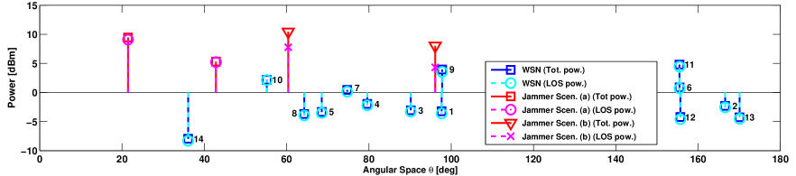
(a) LOS scenario for WSN.

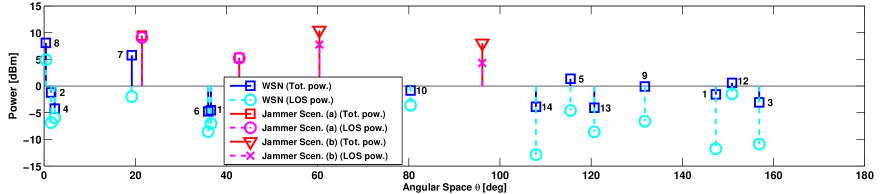
(b) Intermediate scenario for WSN.

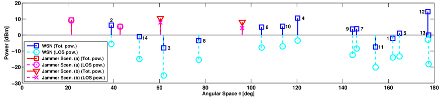
(c) NLOS scenario for WSN.

Figure 1: Simulated setups for fusion rules comparison. Overall ($\beta_{k}$) and LOS ($b_{k}^{2}\,\beta_{k}$) received power ($\mathrm{dBm}$) per antenna at the DFC vs. $\theta$ ($\mathrm{deg}$) in a WSN with $K=14$ sensors (blue “$\square$” and cyan “$\circ$” markers, resp.). Each subfigure also reports the overall ($\beta_{\ell,J}$) and LOS ($b_{\ell,J}^{2}\,\beta_{\ell,J}$) received power ($\mathrm{dBm}$) per antenna at the DFC vs. $\theta$ ($\mathrm{deg}$) of a distributed jammer with $r=2$ in scenarios ($a$) (LOS jammer scenario, red “$\square$” and magenta “$\circ$” markers, resp.) and ($b$) (weak-LOS jammer scenario, red “$\nabla$” and magenta “$\times$” markers, resp.).

VI-B Fusion Rules Comparison

$P_{D_{0}}$ vs. noise level $\sigma_{w}^{2}$ (No-interference): First, the scenario with no jammer is addressed. In Figs. 2, 3 and 4, we show $P_{D_{0}}$ vs. $\sigma_{w}^{2}$, under the constraint $P_{F_{0}}=0.01$ for the “LOS”, “Intermediate” and “NLOS” setups in Figs. 1a, 1b and 1c, respectively ($K=14$ sensors and $N\in\{2,6\}$ antennas at the DFC). Clearly, LLR performs the best among all the considered rules. Secondly, WL rules are very close to the LLR in the “LOS” setup (indeed in the conditionally i.i.d. case and at high SNR, for a LOS condition it approximately holds $\underline{\bm{z}}_{\,{\scriptscriptstyle\mathrm{WL}},i}\propto(\underline{\widetilde{\bm{A}}}(\bm{\theta})\,\underline{\widetilde{\bm{A}}}(\bm{\theta})^{\dagger})^{-1}\underline{\widetilde{\bm{A}}}(\bm{\theta})\bm{1}_{k}$, that is WL rules both approximate through right-pseudoinverse operation a counting rule, being optimal in this specific scenario) with increasing performance loss in the “Intermediate” and “NLOS” setups, respectively. Such a trend is in agreement with Lem. 1, which states that as NLOS assumption is verified, the optimum statistic should possess a dependence on $\left\|\bm{y}\right\|^{2}$, which is not the case of WL rules. Also, IGMM, IS and NLOS rules have a performance behaviour in line with the asymptotic equivalences shown in Sec. III-F. Clearly, NLOS setup is such that performance of IGMM, IS and NLOS rules (almost) coincide. On the other hand, in the LOS scenario, IS and IGMM rules are very close (the “weak-LOS” assumption is almost satisfied), while NLOS rule experiences a certain performance loss. Finally, we underline that the benefit of improved number of antennas is only experienced by LLR, WL and IGMM rules. Differently, NLOS and IS rules do benefit of a larger DFC array only in the case of low SNR or NLOS setup. This can be attributed to the fact that only in these conditions there is no significant (pseudo-)covariance structure change between the two hypotheses (see (8) and (9)). Then NLOS and IS rules, not exploiting (at least) a second-order characterization of $\bm{y}|\mathcal{H}_{i}$, are not able to benefit from increase of $N$ in the remaining cases.

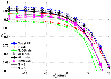
Figure 2: $P_{D_{0}}$ vs. $\sigma_{w}^{2}$ ($\mathrm{dBm}$) for a WSN with $K=14$, LOS setup; $P_{F_{0}}=(0.01)$; $N\in\{2,6\}$ antennas at the DFC.

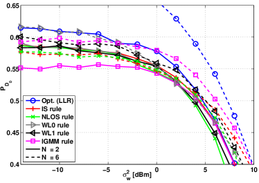
Figure 3: $P_{D_{0}}$ vs. $\sigma_{w}^{2}$ ($\mathrm{dBm}$) for a WSN with $K=14$, Intermediate setup; $P_{F_{0}}=(0.01)$; $N\in\{2,6\}$ antennas at the DFC.

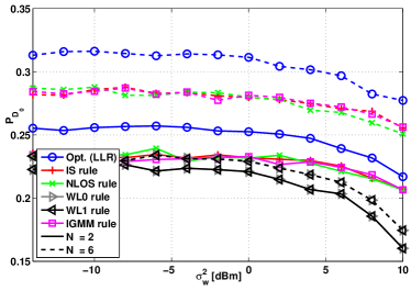
Figure 4: $P_{D_{0}}$ vs. $\sigma_{w}^{2}$ ($\mathrm{dBm}$) for a WSN with $K=14$, NLOS setup; $P_{F_{0}}=(0.01)$; $N\in\{2,6\}$ antennas at the DFC.

$P_{D_{0}}$ vs. noise level $\sigma_{w}^{2}$ (Interference): A similar scenario is shown in Figs. 5, 6 and 7, where we show $P_{D_{0}}$ vs. $\sigma_{w}^{2}$, under the constraint $P_{F_{0}}=0.01$ for the “LOS”, “Intermediate” and “NLOS” setups in Figs. 1a, 1b and 1c, respectively ($K=14$, both jammer scenarios considered), and $N=6$ antennas at the DFC. For the sake of completeness, the performance of clairvoyant LRT are also reported (cf. Eq. (24)). We first notice that IS-GLRT, NLOS-GLRT and IGMM-GLRT outperform IS, NLOS and IGMM rules (whose performance are obtained by ignoring the presence of the jamming signal), respectively, unless there is a significant receive noise $\sigma_{w}^{2}$ (i.e., low SNR); such trend is more apparent when moving to a WSN-DFC channel which experiences a LOS scenario (cf. Fig. 5). Indeed, in such a case, jammer interference suppression may come up at the expenses of (partial) cancellation of some of the sensors contributions. Indeed, in a LOS scenario and at low SNR, jammer interference suppression may not be beneficial as the scenario is noise-dominated. On the other hand, in a LOS scenario and at high SNR, the problem becomes interference-dominated; therefore an effective jammer signal suppression significantly improves performance, even at the expenses of (partial) elimination of some sensors contributions. The sole exception to these considerations is represented by IGMM-GLRT in a NLOS WSN scenario (cf. Fig. 1c), where performance are observed to be worse than its interference-unaware counterpart (i.e., IGMM rule) over all the $\sigma_{w}^{2}$ range considered. Such evidence can be attributed to the overlapping of unknown parameter support under the two hypotheses, due to $\sigma_{J}^{2}$ (cf. Sec. IV-E), which does not allow to achieve satisfactory performance.

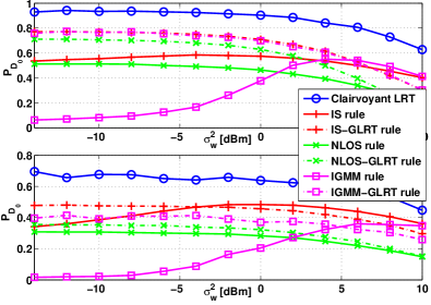
Figure 5: $P_{D_{0}}$ vs. $\sigma_{w}^{2}$ ($\mathrm{dBm}$) for a WSN with $K=14$ sensors. LOS setup with jammer interference ($r=2$): top figure - scenario ($a$) (LOS jam.); bottom figure - scenario ($b$) (weak-LOS jam.); $P_{F_{0}}=0.01$. $N=6$ antennas at the DFC.

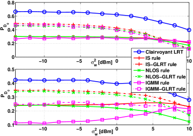
Figure 6: $P_{D_{0}}$ vs. $\sigma_{w}^{2}$ ($\mathrm{dBm}$) for a WSN with $K=14$ sensors. Intermediate setup with jammer interference ($r=2$): top figure - scenario ($a$) (LOS jam.); bottom figure - scenario ($b$) (weak-LOS jam.); $P_{F_{0}}=0.01$. $N=6$ antennas at the DFC.

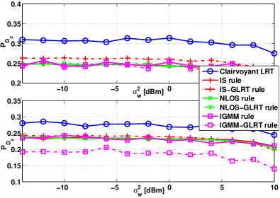
Figure 7: $P_{D_{0}}$ vs. $\sigma_{w}^{2}$ ($\mathrm{dBm}$) for a WSN with $K=14$. NLOS setup with jammer interference ($r=2$): top figure - scenario ($a$) (LOS jam.); bottom figure - scenario ($b$) (weak-LOS jam.); $P_{F_{0}}=0.01$. $N=6$ antennas at the DFC.

$P_{D_{0}}$ vs. number of antennas $N$ (Interference): The benefits of increasing the number of antennas on jammer suppression capabilities for the designed rules are illustrated in Figs. 8, 9, and 10, respectively. More specifically, it is shown $P_{D_{0}}$ vs. $N$, under the constraint $P_{F_{0}}=0.01$ and $\sigma_{w}^{2}=0\,\mathrm{dBm}$ for the “LOS”, “Intermediate” and “NLOS” setups in Figs. 1a, 1b and 1c, respectively. First of all, we notice that $P_{D_{0}}$ for all the “interference-aware” fusion rules increases with $N$. Furthermore, the gain with respect to their corresponding “interference-unaware” counterparts improves as well. This is true in the case of IS-GLRT and NLOS-GLRT for all the scenarios considered, since the considered noise level $\sigma_{w}^{2}$ implies a moderate SNR and due to improved jamming-suppression capabilities with higher $N$. Again, the only exception is given by IGMM-GLRT in the NLOS case, given the overlapping of unknown parameter support under both the hypotheses due to $\sigma_{J}^{2}$. By looking at the specific example, in the LOS WSN scenario, the IGMM-GLRT has the best trend with the number of antennas, as significant pseudo-covariance structure change in the hypotheses is implied in such scenario (therefore second-order characterization of $\bm{y}|\mathcal{H}_{i}$ is beneficial). Differently, in the “Intermediate” and “NLOS” WSN setups, IS-GLRT and NLOS-GLRT represent the best alternatives, with IS-GLRT slightly outperforming NLOS-GLRT.

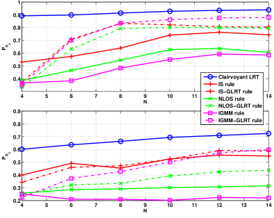
Figure 8: $P_{D_{0}}$ vs. $N$ for a WSN with $K=14$, $\sigma_{w}^{2}=0\,\mathrm{dBm}$. LOS setup with jammer interference ($r=2$): top figure - scenario ($a$) (LOS jam.); bottom figure - scenario ($b$) (weak-LOS jam.); $P_{F_{0}}=0.01$.

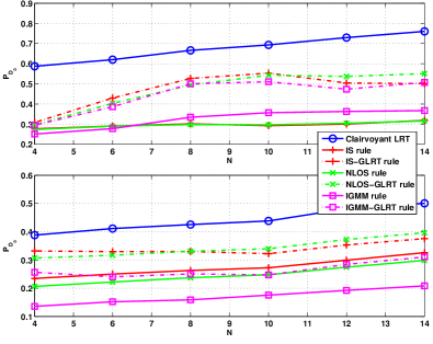
Figure 9: $P_{D_{0}}$ vs. $N$ for a WSN with $K=14$, $\sigma_{w}^{2}=0\,\mathrm{dBm}$. Intermediate setup with jammer interference ($r=2$): top figure - scenario ($a$) (LOS jam.); bottom figure - scenario ($b$) (weak-LOS jam.); $P_{F_{0}}=0.01$.

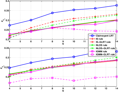
Figure 10: $P_{D_{0}}$ vs. $N$ for a WSN with $K=14$, $\sigma_{w}^{2}=0\,\mathrm{dBm}$. NLOS setup with jammer interference ($r=2$): top figure - scenario ($a$) (LOS jam.); bottom figure - scenario ($b$) (weak-LOS jam.); $P_{F_{0}}=0.01$.

VII Conclusions

In this paper we studied channel-aware DF in a WSN with interfering sensors whose channels are modelled as Rician and their NLOS components are not known at the DFC (i.e., they are not estimated), focusing on anomaly detection problems. We developed five sub-optimal fusion rules (i.e., IS, NLOS, WL and IGMM rules) in order to deal with the exponential complexity of LRT. For the present setup, the following performance trends have been observed:

• In a WSN with a LOS setup, WL rules represent the best (and more convenient) alternative to the LLR, whereas the same rules suffer from severe performance degradation in a NLOS setup. On the other hand, NLOS rule is mainly appealing in a NLOS setup, as the IS rule, which also achieves satisfactory performance in a weak-LOS condition. Indeed, in the latter case they are both able to exploit an increase in the number of receive antennas, as well as in the case of low SNR. Finally IGMM rule, exploiting a second-order characterization of the received vector under both hypotheses, has the most appealing performance when considering all the three scenarios.

Successively, we considered a scenario with a (possibly distributed) “Rician” jamming interference and tackled the resulting composite hypothesis testing problem within the GLRT framework. More specifically, we developed sub-optimal GLRT-like decision rules which extend IS, NLOS and IGMM rules to the case of subspace interference. With reference to these rules, the following trends have been observed:

• All the considered “interference-aware” rules (IS-GLRT, NLOS-GLRT and IGMM-GLRT) significantly outperform the “interference-unaware” counterparts in the case of a moderate-to-high SNR level and non-negligible LOS condition, as in such case system performance is interference-dominated and thus interference suppression leads to a remarkable gain. Also, it has been shown that all these rules benefit from increase of $N$ for enhanced interference suppression, with the sole exception of IGMM-GLRT in a NLOS case (due to lack of identifiability). Numerical evidence has also underlined the appeal of IGMM-GLRT and IS-GLRT in LOS and Intermediate/NLOS setups, respectively;

Finally, asymptotic equivalences established among all these rules in the case of either interference-free or interference-prone scenarios were confirmed by simulations. Future research tracks will concern theoretical performance analysis of the proposed rules and design of advanced fusion schemes robust to smarter jammers.

In this appendix we will provide the second-order characterization of $\bm{y}|\mathcal{H}_{i}$. The mean vector $\mathbb{E}\{\bm{y}|\mathcal{H}_{i}\}$ is evaluated as:

$$\mathbb{E}\{\bm{y}|\mathcal{H}_{i}\}=\mathbb{E}\{\bar{\bm{H}}\bm{D}^{1/2}\bm{x}+\bm{w}|\mathcal{H}_{i}\}=$$ (70)

$$\mathbb{E}\{\bar{\bm{H}}\}\,\bm{D}^{1/2}\,\mathbb{E}\{\bm{x}|\mathcal{H}_{i}\}=\widetilde{\bm{A}}(\bm{\theta})\,\bm{\rho}_{i}$$ (71)

where we have exploited $\mathbb{E}\{\bm{w}\}=\bm{0}_{N}$ and statistical independence between fading coefficients and sensors decisions, respectively. Finally in Eq. (71) we have recalled the definitions of matrix $\widetilde{\bm{A}}(\bm{\theta})$, whose $k$th column equals $\bm{\mu}_{k}=b_{k}\,\sqrt{\beta_{k}}\,\bm{a}(\theta_{k})$, and of $\bm{\rho}_{i}=\begin{bmatrix}P_{i,1}&\cdots&P_{i,K}\end{bmatrix}^{T}$.

Differently, the covariance matrix is expressed as:

$$\bm{\Sigma}_{\bm{y}|\mathcal{H}_{i}}=$$

$$\mathbb{E}\{(\bm{y}-\widetilde{\bm{A}}(\bm{\theta})\,\bm{\rho}_{i})\,(\bm{y}-\widetilde{\bm{A}}(\bm{\theta})\,\bm{\rho}_{i})^{\dagger}\,|\mathcal{H}_{i}\}=$$ (72)

$$\widetilde{\bm{A}}(\bm{\theta})\,\mathbb{E}\{(\bm{x}-\bm{\rho}_{i})(\bm{x}-\bm{\rho}_{i})^{T}\,|\mathcal{H}_{i}\}\,\widetilde{\bm{A}}(\bm{\theta})^{\dagger}\,+$$

$$\mathbb{E}\{(\bm{H}\,\bm{B}_{s}\,\bm{x})(\bm{H}\,\bm{B}_{\mathrm{s}}\,\bm{x})^{\dagger}\,|\mathcal{H}_{i}\}+\mathbb{E}\{\bm{w}\bm{w}^{\dagger}\}=$$ (73)

$$\widetilde{\bm{A}}(\bm{\theta})\,\bm{\Sigma}_{\bm{x}|\mathcal{H}_{i}}\,\widetilde{\bm{A}}(\bm{\theta})^{\dagger}+$$

$$\mathbb{E}\left\{\left(\sum_{k=1}^{K}\bm{h}_{k}\,\sqrt{\nu_{k}}\,x_{k}\right)\left(\sum_{\ell=1}^{K}\bm{h}_{\ell}^{\dagger}\,\sqrt{\nu_{\ell}}\,x_{\ell}\right)|\mathcal{H}_{i}\right\}+\sigma_{w}^{2}\,\bm{I}_{N}$$ (74)

where $\bm{B}_{s}\triangleq(\bm{I}_{K}-\bm{R}^{2})^{1/2}\bm{D}^{1/2}$ and we recall $\nu_{k}=(1-b_{k}^{2})\beta_{k}$. The second term in Eq. (74) can be simplified as

$$\mathbb{E}\left\{\left(\sum_{k=1}^{K}\bm{h}_{k}\,\sqrt{\nu_{k}}\,x_{k}\right)\left(\sum_{\ell=1}^{K}\bm{h}_{\ell}^{\dagger}\,\sqrt{\nu_{\ell}}\,x_{\ell}\right)|\mathcal{H}_{i}\right\}=$$

$$\sum_{k=1}^{K}\mathbb{E}\{\bm{h}_{k}\,\bm{h}_{k}^{\dagger}\}\,\nu_{k}\,\mathbb{E}\{x_{k}^{2}|\mathcal{H}_{i}\}=\sum_{k=1}^{K}\nu_{k}\,P_{i,k}\,\bm{I}_{N}$$ (75)

which follows from mutual independence of vectors $\bm{h}_{k}$, $k\in\mathcal{K}$. Then, substituting back Eq. (75) in Eq. (74) gives:

$$\bm{\Sigma}_{\bm{y}|\mathcal{H}_{i}}=\widetilde{\bm{A}}(\bm{\theta})\,\bm{\Sigma}_{\bm{x}|\mathcal{H}_{i}}\,\widetilde{\bm{A}}(\bm{\theta})^{\dagger}+\sigma_{e,i}^{2}\,\bm{I}_{N}$$ (76)

where $\sigma_{e,i}^{2}\triangleq[\sum_{k=1}^{K}\nu_{k}\,P_{i,k}+\sigma_{w}^{2}]$. Analogously, we can evaluate the pseudo-covariance of $\bm{y}|\mathcal{H}_{i}$ as

$$\bar{\bm{\Sigma}}_{\bm{y}|\mathcal{H}_{i}}=\mathbb{E}\{(\bm{y}-\widetilde{\bm{A}}(\bm{\theta})\,\bm{\rho}_{i})\,(\bm{y}-\widetilde{\bm{A}}(\bm{\theta})\,\bm{\rho}_{i})^{T}\,|\mathcal{H}_{i}\}$$ (77)

$$=\widetilde{\bm{A}}(\bm{\theta})\,\mathbb{E}\{(\bm{x}-\bm{\rho}_{i})(\bm{x}-\bm{\rho}_{i})^{T}\,|\mathcal{H}_{i}\}\,\widetilde{\bm{A}}(\bm{\theta})^{T}\,+$$

$$\mathbb{E}\{(\bm{H}\,\bm{B}_{\mathrm{s}}\,\bm{x})(\bm{H}\,\bm{B}_{\mathrm{s}}\,\bm{x})^{T}\,|\mathcal{H}_{i}\}$$ (78)

$$=\widetilde{\bm{A}}(\bm{\theta})\,\bm{\Sigma}_{\bm{x}|\mathcal{H}_{i}}\,\widetilde{\bm{A}}(\bm{\theta})^{T}+$$

$$\mathbb{E}\left\{\left(\sum_{k=1}^{K}\bm{h}_{k}\,\sqrt{\nu_{k}}\,x_{k}\right)\left(\sum_{\ell=1}^{K}\bm{h}_{\ell}^{T}\,\sqrt{\nu_{\ell}}\,x_{\ell}\right)|\mathcal{H}_{i}\right\}$$ (79)

since $\mathbb{E}\{\bm{w}\,\bm{w}^{T}\}=\bm{O}_{N}$ (i.e., the noise is assumed circular). Also, it can be shown that the second term in Eq. (79) is a null matrix, since

$$\mathbb{E}\left\{\left(\sum_{k=1}^{K}\bm{h}_{k}\,\sqrt{\nu_{k}}\,x_{k}\right)\left(\sum_{\ell=1}^{K}\bm{h}_{\ell}^{T}\,\sqrt{\nu_{\ell}}\,x_{\ell}\right)|\mathcal{H}_{i}\right\}=$$

$$\sum_{k=1}^{K}\mathbb{E}\{\bm{h}_{k}\,\bm{h}_{k}^{T}\}\,\nu_{k}\,\mathbb{E}\{x_{k}^{2}|\mathcal{H}_{i}\}=\bm{O}_{N}$$ (80)

since the NLOS fading vector $\bm{h}_{k}$ is assumed circular. Therefore the final expression for the pseudo-covariance is:

$$\bar{\bm{\Sigma}}_{\bm{y}|\mathcal{H}_{i}}=\widetilde{\bm{A}}(\bm{\theta})\,\bm{\Sigma}_{\bm{x}|\mathcal{H}_{i}}\,\widetilde{\bm{A}}(\bm{\theta})^{T}$$ (81)

Eq. (81) is not a null matrix, thus motivating augmented form processing.

References

- [1] B. Chen, L. Tong, and P. K. Varshney, “Channel-aware distributed detection in wireless sensor networks,” IEEE Signal Process. Mag., vol. 23, no. 4, pp. 16–26, Jul. 2006.
- [2] B. Chen, R. Jiang, T. Kasetkasem, and P. K. Varshney, “Channel aware decision fusion in wireless sensor networks,” IEEE Trans. Signal Process., vol. 52, no. 12, pp. 3454–3458, Dec. 2004.
- [3] A. Lei and R. Schober, “Coherent Max-Log decision fusion in wireless sensor networks,” IEEE Trans. Commun., vol. 58, no. 5, pp. 1327–1332, May 2010.
- [4] R. Jiang and B. Chen, “Fusion of censored decisions in wireless sensor networks,” IEEE Trans. Wireless Commun., vol. 4, no. 6, pp. 2668–2673, Nov. 2005.
- [5] W. Li and H. Dai, “Distributed detection in wireless sensor networks using a multiple access channel,” IEEE Trans. Signal Process., vol. 55, no. 3, pp. 822–833, Mar. 2007.
- [6] C. R. Berger, M. Guerriero, S. Zhou, and P. K. Willett, “PAC vs. MAC for decentralized detection using noncoherent modulation,” IEEE Trans. Signal Process., vol. 57, no. 9, pp. 3562–3575, Sep. 2009.
- [7] F. Li, J. S. Evans, and S. Dey, “Decision fusion over noncoherent fading multiaccess channels,” IEEE Trans. Signal Process., vol. 59, no. 9, pp. 4367–4380, Sep. 2011.
- [8] D. Ciuonzo, G. Romano, and P. Salvo Rossi, “Optimality of received energy in decision fusion over Rayleigh fading diversity MAC with non-identical sensors,” IEEE Trans. Signal Process., vol. 61, no. 1, pp. 22–27, Jan. 2013.
- [9] K. Umebayashi, J. J. Lehtomaki, T. Yazawa, and Y. Suzuki, “Efficient decision fusion for cooperative spectrum sensing based on OR-rule,” IEEE Trans. Wireless Commun., vol. 11, no. 7, pp. 2585–2595, Jul. 2012.
- [10] S. Yiu and R. Schober, “Nonorthogonal transmission and noncoherent fusion of censored decisions,” IEEE Trans. Veh. Technol., vol. 58, no. 1, pp. 263–273, Jan. 2009.
- [11] X. Zhang, H. V. Poor, and M. Chiang, “Optimal power allocation for distributed detection over MIMO channels in wireless sensor networks,” IEEE Trans. Signal Process., vol. 56, no. 9, pp. 4124–4140, Sep. 2008.
- [12] K. Bai and C. Tepedelenlioglu, “Distributed detection in UWB wireless sensor networks,” IEEE Trans. Signal Process., vol. 58, no. 2, pp. 804–813, Feb. 2010.
- [13] M. K. Banavar, A. D. Smith, C. Tepedelenlioglu, and A. Spanias, “On the effectiveness of multiple antennas in distributed detection over fading MACs,” IEEE Trans. Wireless Commun., vol. 11, no. 5, pp. 1744–1752, May 2012.
- [14] I. Nevat, G. W. Peters, and I. B. Collings, “Distributed detection in sensor networks over fading channels with multiple antennas at the fusion centre,” IEEE Trans. Signal Process., vol. 62, no. 3, Feb. 2014.
- [15] F. Jiang, J. Chen, A. L. Swindlehurst, and J. A. Lopez-Salcedo, “Massive MIMO for wireless sensing with a coherent multiple access channel,” IEEE Trans. Signal Process., vol. 63, no. 12, Jun. 2015.
- [16] D. Ciuonzo, G. Romano, and P. Salvo Rossi, “Channel-aware decision fusion in distributed MIMO wireless sensor networks: Decode-and-fuse vs. decode-then-fuse,” IEEE Trans. Wireless Commun., vol. 11, no. 8, pp. 2976–2985, Aug. 2012.
- [17] D. Ciuonzo, P. Salvo Rossi, and S. Dey, “Massive MIMO channel-aware decision fusion,” IEEE Trans. Signal Process., vol. 63, no. 3, pp. 604–619, Feb. 2015.
- [18] C. Rago, P. K. Willett, and Y. Bar-Shalom, “Censoring sensors: A low-communication-rate scheme for distributed detection,” IEEE Trans. Aerosp. Electron. Syst., vol. 32, no. 2, pp. 554–568, 1996.
- [19] P. Salvo Rossi, D. Ciuonzo, T. Ekman, and K. Kansanen, “Energy detection for decision fusion in wireless sensor networks over Ricean-mixture fading,” in IEEE 8th Sensor Array and Multichannel Signal Processing Workshop (SAM), Jun. 2014, pp. 149–152.
- [20] A. Dogandzic and J. Jin, “Estimating statistical properties of MIMO fading channels,” IEEE Trans. Signal Process., vol. 53, no. 8, pp. 3065–3080, 2005.
- [21] W. Xu, K. Ma, W. Trappe, and Y. Zhang, “Jamming sensor networks: attack and defense strategies,” IEEE Network, vol. 20, no. 3, pp. 41–47, 2006.
- [22] D. Ciuonzo and P. Salvo Rossi, “Decision fusion with unknown sensor detection probability,” IEEE Signal Process. Lett., vol. 21, no. 2, pp. 208–212, Feb. 2014.
- [23] S. M. Kay, Fundamentals of Statistical Signal Processing, Volume 2: Detection Theory. Prentice Hall PTR, Jan. 1998.
- [24] L. L. Scharf, Statistical signal processing. Addison-Wesley Reading, MA, 1991, vol. 98.
- [25] D. Ciuonzo, G. Romano, and P. Salvo Rossi, “Performance analysis of maximum ratio combining in channel-aware MIMO decision fusion,” IEEE Trans. Wireless Commun., vol. 12, no. 9, pp. 4716–4728, Sep. 2013.
- [26] P. J. Schreier and L. L. Scharf, Statistical Signal Processing of Complex-Valued Data: The Theory of Improper and Noncircular Signal. Cambridge, 2010.
- [27] Z. Quan, W.-K. Ma, S. Cui, and A. H. Sayed, “Optimal linear fusion for distributed detection via semidefinite programming,” IEEE Trans. Signal Process., vol. 58, no. 4, pp. 2431–2436, 2010.
- [28] B. Picinbono, “On deflection as a performance criterion in detection,” IEEE Trans. Aerosp. Electron. Syst., vol. 31, no. 3, pp. 1072–1081, Jul. 1995.
- [29] Z. Quan, S. Cui, and A. H. Sayed, “Optimal linear cooperation for spectrum sensing in cognitive radio networks,” IEEE J. Sel. Topics Signal Process., vol. 2, no. 1, pp. 28–40, Feb. 2008.
- [30] K.-C. Lai, Y.-L. Yang, and J.-J. Jia, “Fusion of decisions transmitted over flat fading channels via maximizing the deflection coefficient,” IEEE Trans. Veh. Technol., vol. 59, no. 7, pp. 3634–3640, Jul. 2010.
- [31] D. Gesbert, H. Bölcskei, D. A. Gore, and A. J. Paulraj, “Outdoor MIMO wireless channels: Models and performance prediction,” IEEE Trans. Commun., vol. 50, no. 12, pp. 1926–1934, Dec. 2002.
- [32] E. L. Lehmann and J. P. Romano, Testing statistical hypotheses. Springer Science & Business Media, 2006.
- [33] R. Zhang, T. J. Lim, Y.-C. Liang, and Y. Zeng, “Multi-antenna based spectrum sensing for cognitive radios: A GLRT approach,” IEEE Trans. Commun., vol. 58, no. 1, pp. 84–88, 2010.
- [34] Y. He, T. Ratnarajah, E. H. G. Yousif, J. Xue, and M. Sellathurai, “Performance analysis of multi-antenna GLRT-based spectrum sensing for cognitive radio,” Signal Processing, vol. 120, pp. 580–593, 2016.
- [35] M. Atallah and M. Blanton, Algorithms and Theory of Computation Handbook, Volume 1: General Concepts and Techniques. CRC press, 2009.