Internal rotation of 13 low-mass low-luminosity red giants in the Kepler field

Abstract

Context. The Kepler space telescope has provided time series of red giants of such unprecedented quality that a detailed asteroseismic analysis becomes possible. For a limited set of about a dozen red giants, the observed oscillation frequencies obtained by peak-bagging together with the most recent pulsation codes allowed us to reliably determine the core/envelope rotation ratio. The results so far show that the current models are unable to reproduce the rotation ratios, predicting higher values than what is observed and thus indicating that an efficient angular momentum transport mechanism should be at work. Here we provide an asteroseismic analysis of a sample of 13 low-luminosity low-mass red giant stars observed by Kepler during its first nominal mission. These targets form a subsample of the 19 red giants studied previously Corsaro et al. (2015), which not only have a large number of extracted oscillation frequencies, but also unambiguous mode identifications.

Aims. We aim to extend the sample of red giants for which internal rotation ratios obtained by theoretical modeling of peak-bagged frequencies are available. We also derive the rotation ratios using different methods, and compare the results of these methods with each other.

Methods. We built seismic models using a grid search combined with a Nelder-Mead simplex algorithm and obtained rotation averages employing Bayesian inference and inversion methods. We compared these averages with those obtained using a previously developed model-independent method.

Results. We find that the cores of the red giants in this sample are rotating 5 to 10 times faster than their envelopes, which is consistent with earlier results. The rotation rates computed from the different methods show good agreement for some targets, while some discrepancies exist for others.

1 Introduction

The impact of the Kepler space mission (Borucki et al., 2010; Koch et al., 2010) on diverse aspects of stellar astrophysics has been enormous and revolutionary by many standards. Our understanding of stellar evolution through asteroseismology has improved dramatically, and with this improvement, new challenges have appeared.

Sun-like stars, particularly red giants, exhibit a very rich pulsation pattern (De Ridder et al., 2009; Stello et al., 2009; Hekker et al., 2009). Some of these pulsations can be associated with pressure (p) modes, which are excited stochastically by turbulent convection. These p modes propagate throughout the star with the highest sensitivity to the external convective envelope, as opposed to the internal gravity (g) modes, which propagate only throughout the radiative core and hence are beyond observational reach. The p and g propagation zones generally do not overlap, and the region between them is called the evanescent zone. Modes of mixed character, behaving like g modes in the core and p modes in the envelope, bridge the evanescent zone and have substantial amplitudes in both the core and the envelope (Beck et al., 2011). These modes are extremely useful for obtaining information about the internal rotation of the core. This is possible because rotation induces frequency splittings in the modes, which would otherwise be degenerate in a spherically symmetric star (Ledoux, 1951). Rotation induces a preferential axis in the star, and if the rotation rate is much smaller than the pulsation frequencies, then the splitting $\delta_{nlm}$ of a mode with radial, angular, and azimuthal wavenumbers $n,l,m$ can be computed as (see, e.g., Aerts et al., 2010,  )

$$\delta_{nlm}=m\,\beta_{nl}\int_{0}^{R_{*}}K_{nl}(r)\,\Omega(r)\,\mathrm{d}r,$$ (1)

where the kernel $K_{nl}(r)$ and $\beta_{nl}$ are functions of the vertical and horizontal material displacement eigefunctions $\xi_{r}(r)$ and $\xi_{h}(r)$ (see Section 3 for more details). Thus, rotation lifts the azimuthal wave number degeneracy of the modes.

The milestone work of Beck et al. (2012) on red giants, using data obtained by the Kepler space telescope, took advantage of the detection of rotationally split mixed modes in KIC 8366239 and concluded that the stellar core spins about ten times faster than the envelope. In the same year, Mosser et al. (2012) presented the core rotation of a sample of 300 red giants, establishing that the cores slow down significantly during the last stages of the red giant branch. A number of other studies followed. Most notably, Deheuvels et al. (2012) determined a core/envelope rotation rate ratio of about five for a star in the lower giant branch observed by Kepler, Deheuvels et al. (2014) computed the rotation rate ratio of six subgiants and young red giants, Deheuvels et al. (2015) obtained rotations rates for seven red giants in the secondary clump, and very recently, the work by Di Mauro et al. (2016) resolved the core rotation better than previous studies. In all these cases, the rotation rate of the core does not match the expectations of current angular momentum theories. Indeed, according to our current understanding of the evolution of the angular momentum in stellar interiors, the core is expected to spin up considerably as it contracts in stars at this stage of evolution. Cantiello et al. (2014) explicitly showed the inadequacy of current models in reproducing the observed slow rotation of the core in RGB stars, even after magnetic effects were included. It is then clear that a very effective mechanism for angular momentum transport is at work. Internal gravity waves are capable of transferring considerable amounts of angular momentum (Rogers, 2015; Alvan et al., 2013), which provides a suitable explanation for ‘anomalous’ rotation rates in other types of stars, such as those reported by Kurtz et al. (2014); Saio et al. (2015), and Triana et al. (2015). However, Fuller et al. (2014) showed that this mechanism falls short of explaining the observed rotation rate ratios in stars on the red giant branch. However, mixed modes can also transport angular momentum, as demonstrated recently by Belkacem, K. et al. (2015). According to this study, the mixed-mode wave heat flux has an appreciable effect on the mean angular momentum in the inner regions of the star.

The methods used to obtain the internal rotation rates in red giant stars have seen a number of developments well worth mentioning here. The way to proceed, after the mode detection and identification process (see, e.g., Corsaro et al., 2015) is usually to develop a seismic model of the star with oscillation frequencies that are as similar as possible to the observed frequencies. This process is computationally expensive as a large number of evolutionary tracks with different stellar parameters need to be computed. A seismic model provides oscillation kernels that allow the application of inversion techniques (see Sect. 3) to determine the approximate rotation rates in different regions of the star. This is the approach taken by Deheuvels et al. (2012, 2014), Triana et al. (2015), and Di Mauro et al. (2016).

Goupil et al. (2013) developed a powerful method that allows estimating the rotation rates of both core and envelope, without recurring to any seismic model, by considering the relative amounts of ‘trapping’ of a set of mixed modes, which as they showed are linearly related to the rotational splittings $\delta$ (see Section 2). The method relies solely on observed quantities as inputs and particularly, on an estimate of the asymptotic period spacing $\Delta\Pi_{1}$ that pure high-order g modes would have in the asymptotic regime (Mosser, B. et al., 2012).

This latter approach was taken by Deheuvels et al. (2015) in their sample of seven core He-burning red giants. In that study, a seismic model was obtained for one of the stars in the sample (KIC 7581399) and was used to compute rotation rates through inversions. Then the authors adapted the method of Goupil et al. (2013), and the rotation rates thus obtained were in very good agreement with the inversions based on the seismic model. After assessing the validity of the Goupil approach in this way, no further seismic modeling was attempted for the other targets, and the corresponding rotation rates reported come solely from the use of the adapted method.

Mosser et al. (2015) provided additional insight into the relationship between the relative amount of trapping of a mode (quantified by the parameter $\zeta$) and the observed period spacing $\Delta P$ between consecutive mixed modes. The modification of Goupil’s formula introduced by Deheuvels et al. (2015) is exactly the same expression as was found by Mosser et al. (2015) to represent the ratio $\Delta P/\Delta\Pi_{1}$.

The model-independent method used by Goupil et al. (2013) has been compared with inversions based on seismic models for only two targets: the core helium-burning red giant KIC7581399 (Deheuvels et al., 2015), and the early red giant KIC4448777 (Di Mauro et al., 2016). Although a wider comparison of the method using targets in different evolutionary stages is desirable, we offer comparisons of the model-independent method against inversions for our 13 targets, which share similar evolutionary stages with KIC4448777. Our targets are a subset of the original selection of 19 low-mass, low-luminosity red giants studied by Corsaro et al. (2015) using the Bayesian inference technique Diamonds (Corsaro, E. & De Ridder, J., 2014) to detect and identify pulsation frequencies. Pérez Hernández et al. (2016) performed a grid-based search for models designed specifically to constrain the age, mass, and initial helium content of all 19 targets. In the present work we search for optimal seismic models for the 13 targets that exhibit rotational splittings (Section 5) and employ Bayesian inference and inversion techniques (Section 3) to obtain average rotation rates. We compare these results with those obtained by the model-independent method as implemented by Deheuvels et al. (2015) and by Mosser et al. (2015) using their expressions for the trapping parameter $\zeta$ (Section 6). Additionally, we use the idea proposed recently by Klion & Quataert (2016) that provides a way to localize the differential rotation of a red giant (whether in the radiative core or in the convective envelope of the star), provided that the rotation rate of the envelope is known by other means.

2 Rotation rate averages using the trapping parameter $\zeta$

The parameter $\zeta$ gives an indication of how strongly a given stellar pulsation mode is localized, or‘trapped’, inside the radiative core. It is defined as the ratio of the mode inertia computed within the g -mode cavity $I_{g}$ (Goupil et al., 2013) to the total mode inertia $I$:

$$\zeta\equiv\frac{I_{g}}{I}=\frac{\int_{r_{1}}^{r_{2}}\rho r^{2}\left[\xi_{r}^{2}+l(l+1)\xi_{h}^{2}\right]\,\mathrm{d}r}{\int_{0}^{R_{*}}\rho r^{2}\left[\xi_{r}^{2}+l(l+1)\xi_{h}^{2}\right]\,\mathrm{d}r}.$$ (2)

$\begin{array}[]{cc}\includegraphics[width=195.12767pt]{rotker1.eps}&\includegraphics[width=195.12767pt]{rotker2.eps}\\ \end{array}$

Figure 1: Rotational kernels of two dipole modes with different values of the trapping parameter $\zeta$ (from the best model of KIC007619745). The left panel shows the central region, and the right panel shows the region near the surface.

In the expression above, $\rho$ is the density, $r_{1}$ and $r_{2}$ are the turning points of the g -mode cavity, $l$ is the angular wave number of the mode, $\xi_{r}$ and $\xi_{h}$ are the vertical and horizontal material displacement eigenfunctions, respectively, and $R_{*}$ is the stellar radius (Aerts et al., 2010).

Figure 1 shows the rotational kernels $K_{nl}$ of two mixed modes with different $\zeta$ using a seismic model for KIC007619745. Modes with $\zeta$ close to one are gravity-dominated mixed modes, while modes with $\zeta$ close to 0.5 correspond to pressure-dominated mixed modes.

The rotational splittings $\delta_{i}$ are linearly related to $\zeta_{i}$ for each mode $i,$ as shown by Goupil et al. (2013), which we also refer to for further details. The coefficients of this linear relationship are related directly to the rotational averages across the core and the envelope through

$$\delta=\left(\frac{\Omega_{g}}{2}-\Omega_{p}\right)\zeta+\Omega_{p},$$ (3)

where $\Omega_{p}$ represents the average rotation rate in the envelope (approximated by the p -mode cavity), and $\Omega_{g}$ represents the average rotation rate in the radiative core (approximated by the g -mode cavity). Following Goupil et al. (2013), they are defined as

$$\Omega_{g}=\frac{\int_{0}^{r_{2}}K(r)\,\Omega(r)\,\mathrm{d}r}{\int_{0}^{r_{2}}K(r)\,\mathrm{d}r}$$ (4)

for the core, and

$$\Omega_{p}=\frac{\int_{r_{2}}^{R_{*}}K(r)\,\Omega(r)\,\mathrm{d}r}{\int_{r_{2}}^{R_{*}}K(r)\,\mathrm{d}r}$$ (5)

for the envelope, where $r_{2}$ is the outer turning point in the g resonant cavity and $K(r)$ is the rotational kernel of a mixed-mode. Our tests with the rotational profiles considered in Section 4 show that while the core averages are essentially independent of the particular mixed-mode chosen, the envelope averages differ appreciably across modes with $\zeta\gtrsim 0.9$ (i.e., gravity-dominated modes). Using kernels from mixed modes with $\zeta\lesssim 0.85$ results in envelope averages with minimal variability.

2.1 Estimation of the trapping parameter $\zeta$

The expression for $\zeta$ given by Eq. (2) in principle requires knowing the material displacement eigenfunctions $\xi_{r,h}(r)$ for each mode, which are only available after the computationally expensive process of deriving a seismic model of the star. However, Goupil et al. (2013) used an asymptotic analysis method based on the work of Shibahashi (1979) to show that $\zeta$ can in principle be estimated using observational data alone. The expression for $\zeta$ was later refined by Deheuvels et al. (2015) and Mosser et al. (2015). In what follows, we briefly recall the method and the main formulae, we refer to the original works for further details.

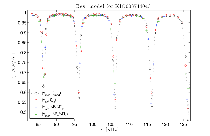
Figure 2: Trapping parameter as described by the true model, $\zeta_{\mathrm{mod}}$ (Eq. 2) as a function of the true frequencies $\nu_{\mathrm{mod}}$ (dashed black line and black circles). Red circles represent the trapping parameter $\zeta_{\mathrm{as}}$ as approximated by Eqs. 11 and 8 and using $\nu_{\mathrm{as}}$ for the mode frequencies as determined by Eq. 6. The scaled period spacing $\Delta P/\Delta\Pi_{1}$ between any two consecutive true frequencies $\nu_{\mathrm{mod},1}$ and $\nu_{\mathrm{mod},2}$ is plotted at the abscissa $\nu_{\Delta P}=2/(\nu^{-1}_{\mathrm{mod},1}+\nu^{-1}_{\mathrm{mod},2})$ (blue crosses). $\Delta P_{\nu}$ represent the interpolated value of the two adjacent period spacings around each frequency $\nu_{\mathrm{mod}}$ (green crosses).

The method consists of finding aproximate JWKB solutions for the material displacement eigenfunctions $\xi_{r,h}(r)$ in the two separate p and g cavities of the star. Matching the solutions in the evanescent zone requires (Unno, 1989)

$$\tan\theta_{p}=q\,\tan\theta_{g},$$ (6)

where $q$ is the coupling constant between the p- and g-mode cavities, and the phases $\theta_{p,g}$ are defined through

$$\theta_{g}=\int_{r_{1}}^{r_{2}}k_{r}\,\mathrm{d}r,\,\,\theta_{p}=\int_{r_{3}}^{r_{4}}k_{r}\,\mathrm{d}r,$$ (7)

where $r_{3}$ and $r_{4}$ are the inner and outer turning points of the p-mode cavity. According to Mosser, B. et al. (2012), asymptotic analysis yields

$$\theta_{p}=\frac{\pi}{\Delta\nu}(\nu-\nu_{p}),\,\,\theta_{g}=\pi\left(\frac{1}{\Delta\Pi_{1}\,\nu}-\epsilon_{g}\right),$$ (8)

where $\nu_{p}$ is the frequency of the theoretical $l=1$ pure p modes, which are related to the radial ($l=0$) modes $\nu_{n,0}$ through

$$\nu_{p}=\nu_{n,0}+\left(\frac{1}{2}-d_{01}\right)\Delta\nu.$$ (9)

In turn, the radial modes can be expressed as a function of the radial order $n$ involving the parameters $\epsilon_{p}$, $\alpha$, and the large frequency separation $\Delta\nu$ as follows (Mosser, B. et al., 2013):

$$\nu_{n,0}=\left[n+\epsilon_{p}+\frac{\alpha}{2}(n-n_{\mathrm{max}})^{2}\right]\Delta\nu,$$ (10)

where $n_{\mathrm{max}}\equiv\nu_{\mathrm{max}}/\Delta\nu-\epsilon_{p}$. The approximate expression for the trapping parameter, denoted here as $\zeta_{\mathrm{as}}$ , reads

$$\zeta_{\mathrm{as}}=\left[1+\frac{\nu^{2}\,\Delta\Pi_{1}}{q\,\Delta\nu}\frac{\cos^{2}\theta_{g}}{\cos^{2}\theta_{p}}\right]^{-1}.$$ (11)

A total of seven parameters are required here: the coupling constant $q$, the offsets $\epsilon_{p,g}$, the mean large frequency separation $\Delta\nu$, the asymptotic period spacing $\Delta\Pi_{1}$, $\alpha,$ and $d_{01}$. In practice, the optimal parameters $\epsilon_{p}$, $\alpha$, and $\Delta\nu$ are determined first by fitting the observed radial modes to Eq. 10. Then, the optimal parameters $q$, $\Delta\Pi_{1}$, $\epsilon_{g}$, and $d_{01}$ that best reproduce the observed $l=1$ mode frequencies can be found by a downhill simplex method. This requires solving Eq. 6 for the mode frequencies $\nu$ at each search step with a particular $(q,\,\Delta\Pi_{1},\,\epsilon_{g},\,d_{01})$ combination, using a Newton method to find the roots of the equation, for example.

The observed rotational splittings $\delta$ are expected to be linearly related to $\zeta_{\mathrm{as}}$ , and a linear fit of $\delta$ as a function of $\zeta_{\mathrm{as}}$ leads to an estimate of the average envelope rotation and the envelope core rotation through Eq. 3.

Mosser et al. (2015) obtained a result in their search of an expression for the mixed-mode relative period spacings $\Delta P/\Delta\Pi_{1}$ that exactly matched the expression for $\zeta_{\mathrm{as}}$ (Eq. 11) found by Deheuvels et al. (2015). Thus, we have

$$\zeta_{\mathrm{as}}=\frac{\Delta P}{\Delta\Pi_{1}}.$$ (12)

The above is a reflection of the fact that the rotational splittings follow the same distribution as the period spacing, because both are determined by the coupling between pressure and gravity terms. As a bonus, Equation 12 provides a simple and direct way to estimate $\zeta$ from observations without the need of the optimal parameters mentioned above (which can be slightly time consuming computationally) with the exception of $\Delta\Pi_{1}$. Some care must be taken because the period spacing between two consecutive mixed dipole modes $\Delta P(n,n+1)=\nu^{-1}_{n+1}-\nu^{-1}_{n}$ is defined properly at $\nu=2/(\nu^{-1}_{n+1}+\nu^{-1}_{n})\equiv\nu_{\Delta P}$. In order to assign a $\Delta P$ to each mode $\nu_{n}$, we therefore interpolate the two adjacent period spacings $\Delta P(n,n+1)$ and $\Delta P(n-1,n)$ linearly. Similarly, when performing linear fits of $\delta$ vs. $\zeta_{\mathrm{as}}$, it is advisable to also include the interpolated rotational splitting at each location $\nu_{\Delta P}$ using the two correspondingly adjacent values of $\delta$ to minimize biases, see Fig. 6.

In Fig. 2 we show that the trapping parameter $\zeta_{\mathrm{mod}}$ as derived from a known seismic model is indeed well approximated by either $\zeta_{\mathrm{as}}$ derived using asymptotic analysis, Eq. 11, or by the simpler expression given by Eq. 12.

Assuming that the errors on the frequencies and the splittings are normally distributed, we can sample randomly from them and proceed to compute interpolated splittings and spacings as explained earlier. A linear fit to these points leads to estimates of $\Omega_{g}$ and $\Omega_{p}$ according to Eq. 3. By repeating these steps many times, we can obtain the distributions associated with $\Omega_{g}$ and $\Omega_{p}$ and their associated errors.

2.2 Bayesian inference

If a seismic model providing the oscillation eigenfunctions $\xi_{r,h}$ is available, the trapping parameter can be computed from Eq. 2, which we denote now as $\zeta_{\mathrm{mod}}$. With two sets of inputs, that is, the splittings $\delta_{i}$ and the trapping parameters $\zeta_{\mathrm{mod},i}$, we can set out to perform a Bayesian fit using Eq. 3 as the model. To accomplish this, we first compute a Gaussian log-likelihood function defined as (see also Corsaro et al., 2013)

$$\Lambda(\Omega_{g},\,\Omega_{p})=\Lambda_{0}-\frac{1}{2}\sum^{N}_{i=1}\left[\frac{\Delta_{i}(\Omega_{g}\,,\Omega_{p})}{\epsilon_{i}}\right]^{2}\,,$$ (13)

where $N$ is the total number of rotational splittings $\delta_{i}$ from the observations (one for each m-multiplet of mixed modes), $\Delta_{i}(\Omega_{g},\,\Omega_{p})$ are the residuals given as the difference between the observed and the modeled splittings, $\epsilon_{i}$ the corresponding uncertainty, and

$$\Lambda_{0}=-\sum^{N}_{i=1}\ln{\sqrt{2\pi}\,\epsilon_{i}}\,,$$ (14)

a constant term. We multiply the likelihood distribution by the prior distributions (uniform or flat in this case, in the range $\Omega_{g}\in\left[2,8\right]\,\mu$Hz, and $\Omega_{p}\in\left[0,3\right]\,\mu$Hz), obtaining a posterior probability density distribution. By marginalizing the bidimensional posterior into two one-dimensional probability density distributions, we obtain estimates for $\Omega_{p}$ and $\Omega_{g}$ that are the medians of the two one-dimensional distributions. The corresponding error bars are the Bayesian credible intervals computed as explained in Corsaro et al. (2013). This statistical approach may provide similar results to a least-squares fit, but it is conceptually very different. One of the main differences is that it is able to incorporate any a priori knowledge on the estimated parameters that we may have, for instance, in the form of the prior distributions described above.

An example of this Bayesian fit is shown in Figure 3 for the star KIC007619745 (solid orange line), with 1$\sigma$ error bars overlaid. The results from this method for all targets are included in Table 1 under the ‘Bayes’ heading.

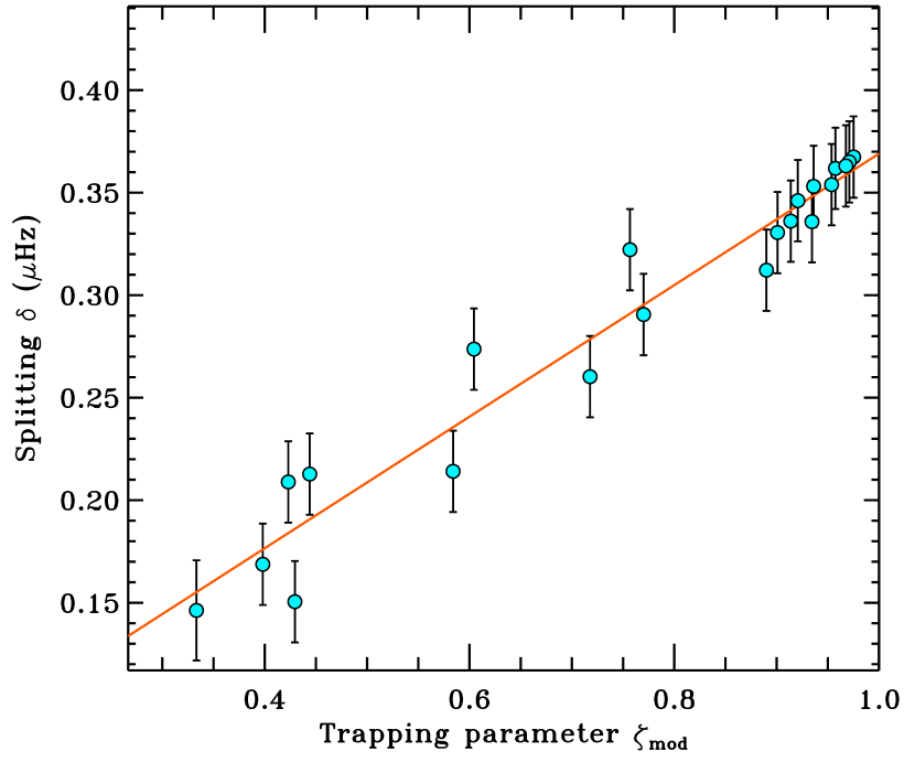
Figure 3: Illustrative use of a Bayesian fit to compute rotation rates for KIC007619745. The trapping parameters $\zeta_{\mathrm{mod}}$ are obtained from the eigenmodes as computed by GYRE.

3 Inversion methods

In this section we present the methods we used to obtain rotation rate averages, which are all based on the oscillation kernels provided by the seismic models described in Section 5. Our treatment is based on Aerts et al. (2010), who offered an extended presentation of the methods discussed below.

The so-called forward problem states that the rotational splittings $\delta_{nlm}$ of an oscillation mode with radial, angular, and azimuthal wavenumbers $n,l,m$ can be computed through Eq. (1). Explicitely, the kernels are computed from the material displacement eigenfunctions via

$$K_{nl}=\frac{1}{I}\left[\xi_{r}^{2}+l(l+1)\,\xi_{h}^{2}-2\xi_{r}\xi_{h}-\xi_{h}^{2}\right]r^{2}\rho,$$ (15)

where $I$ is the mode inertia (see Eq. 2). The constant $\beta_{nl}$ is given by

$$\beta_{nl}=\frac{1}{I}\int_{0}^{R_{*}}\left[\xi_{r}^{2}+l(l+1)\xi_{h}^{2}-2\xi_{r}\xi_{h}-\xi_{h}^{2}\right]r^{2}\rho\,\mathrm{d}r.$$ (16)

The inverse problem consists of determining the unknown inversion coefficients $c_{i}(r)$ satisfying

$$\bar{\Omega}(r)=\sum_{i=1}^{M}c_{i}(r)\frac{\delta_{i}}{m\,\beta_{i}},$$ (17)

where $\bar{\Omega}(r)$ is the predicted internal rotation rate of the star, $M$ is the number of observed splittings, and $i$ denotes the collective indices $(n,l,m)$. Clearly, the inversion coefficients $c_{i}$ are not determined by Eq. 17, which just states a linear relationship between the observed splittings and the predicted rotation profile. The $c_{i}(r)$ are determined by minimizing the difference between observed and predicted splittings, by minimizing of the resulting uncertainties, or by adjusting the shape of the averaging kernels, as discussed below.

The approximate rotational profile $\bar{\Omega}(r)$ can be expressed in terms of the true profile $\Omega(r)$ by means of the averaging kernels $\mathcal{K}(r^{\prime},r)$, which are related to the kernels $K_{i}(r)$ through $\mathcal{K}(r^{\prime},r)=\sum_{i=1}^{M}c_{i}(r^{\prime})K_{i}(r)$ and fulfill

$$\bar{\Omega}(r^{\prime})=\int_{0}^{R_{*}}\mathcal{K}(r^{\prime},r)\,\Omega(r)\,\mathrm{d}r.$$ (18)

The averaging kernels $\mathcal{K}(r^{\prime},r)$ should be localized around $r^{\prime}$ as much as possible, ideally resembling a delta function $\delta(r^{\prime},r)$. It is usually assumed that the observational errors $\epsilon_{i}$ are uncorrelated (as in, e.g., Deheuvels et al. (2012) or Di Mauro et al. (2016)), so that the variance of the predicted rotation rates can be estimated as

$$\sigma^{2}\left[\bar{\Omega}(r)\right]=\sum_{i=1}^{M}c_{i}^{2}(r)\,\left(\frac{\epsilon_{i}}{\beta_{i}}\right)^{2}.$$ (19)

The expression above accounts for the errors originating from the observations alone; it does not account for the inherent errors of the inversion process itself.

3.1 Two-zone inversion models

To obtain approximate averages of the core and envelope rotation rates, we can make use of simple two-zone models where we assume an inner zone extending from the stellar center to $r/R_{*}=x_{c}$ and an outer zone extending from $r/R_{*}=x_{c}$ all the way to stellar surface at $r/R_{*}=1$, both zones rotating uniformly with rates $\Omega_{g}$ and $\Omega_{p}$ , respectively. Our 13 targets happen to be approximately at the same evolutionary stage, and therefore it is not surprising that our seismic models show all their evanescent zones located at approximately the same radial locations (scaled by stellar radius) We have chosen $x_{c}$ to coincide with the base of the convection zone for each target, see Figure 4. We can determine the inversion coefficients $c_{i}$ associated with each zone by finding the optimal $\Omega_{g}$ and $\Omega_{p}$ that minimize

$$\chi^{2}=\sum_{i=1}^{M}\left(\frac{\bar{\delta}_{i}-\delta_{i}}{\epsilon_{i}}\right)^{2},$$ (20)

where $\epsilon_{i}$ are the observation errors and $\bar{\delta}_{i}$ are the predicted splittings associated with the two-zone rotation profile composed of $\Omega_{g}$ and $\Omega_{p}$. The averages are determined by enforcing $\partial(\chi^{2})/\partial\Omega_{g,p}=0$ after substituting $\chi^{2}$ using Eqs. 1 and 20. Results from this method, with kernels from the seismic models discussed below, are presented on Table 1 under the ‘Two-zone’ heading.

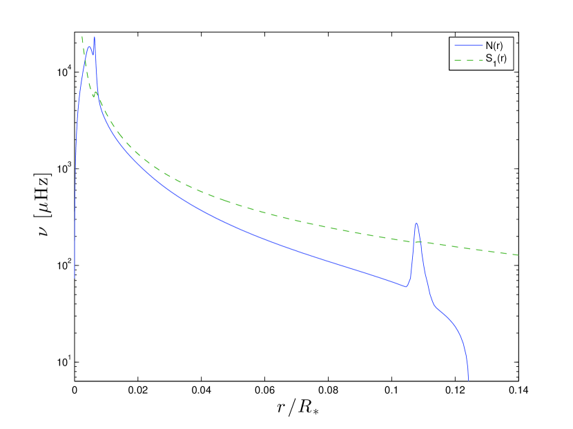
Figure 4: Propagation diagram of the best model of KIC 007619745. The Brunt-Väisälä frequency $N(r)$ is plotted as a solid blue curve, and the $l=1$ Lamb frequency $S_{1}(r)$ is plotted as a dashed green curve. p-modes with frequency $\nu$ are evanescent in the region where $\nu<S_{1}(r)$. Similarly, g-modes are evanescent wherever $\nu>N(r)$. The core-envelope boundary in our two-zone models is located at $r_{c}\approx 0.1R_{*}$ , which usually lies in the evanescent zone common to both p- and g-modes. The peak of $N(r)$ near $r/R_{*}=0.11$ is associated with a chemically inhomogeneous layer in the radiative zone, left behind by convection as the boundary moves upward.

3.2 Subtractive optimally localized averaging

One of the differences between the subtractive optimally localized averaging (SOLA) method (Pijpers & Thompson, 1994) and the method described above is that with SOLA we do not minimize $\chi^{2}$ , but instead, the method chooses the optimal linear combination of the inversion coefficients $c_{i}$ such that the averaging kernels $\mathcal{K}(r^{\prime},r)$ resemble a given target function $T(r^{\prime},r)$ as closely as possible while keeping the variance $\sigma^{2}(\bar{\Omega})$ low. Thus, we minimize

$$\int_{0}^{R_{*}}\left[\mathcal{K}(r^{\prime},r)-T(r^{\prime},r)\right]^{2}\mathrm{d}r+\mu\sum_{i=1}^{M}c_{i}^{2}(r^{\prime})\,\epsilon_{i}^{2}$$ (21)

at each $r^{\prime}$, with the additional constraint $\int_{0}^{R_{*}}\mathcal{K}(r^{\prime},r)\,\mathrm{d}r=1$. The target function that we have chosen in this study is a Gaussian with unit norm, centered on $r=r^{\prime}$ with adjustable width $s$:

$$T(r^{\prime},r)=N\,\mathrm{e}^{-{\left(\frac{r^{\prime}-r}{s}\right)}^{2}},$$ (22)

$N$ being a normalization factor. In addition to the free parameter $\mu$ in Eq. 21, we can also adjust the shape of the target function $T$ by adjusting the width $s$. The problem reduces to solving the linear set of $M$ equations ($i=1,\ldots,M$) for each radial location $r^{\prime}$:

$$\sum_{k=1}^{M}W_{ik}\,c_{k}(r^{\prime})=\int_{0}^{R_{*}}K_{i}(r)\,T(r^{\prime},r)\,\mathrm{d}r,$$ (23)

where $W_{ik}=\int_{0}^{R_{*}}K_{i}(r)\,K_{k}(r)\,\mathrm{d}r+\mu\,\delta_{ik}\,\epsilon_{i}^{2}$, together with the constraint $\sum_{k}c_{k}(r^{\prime})=1,$ which is implemented via Lagrange multipliers. Given a set of kernels $K_{i}(r)$ and the two parameters $(s,\leavevmode\nobreak\ \mu)$, the inversion coefficients $c_{i}(r^{\prime})$ are determined by solving the set of $M$ equations given by Eq. 23. We note that the observed splittings are not involved in determining the $c_{i}(r^{\prime})$, they determine the predicted rotation rate $\bar{\Omega}(r^{\prime})$ via Eq. 17.

4 Testing the methods

Before applying the methods described above to determine rotation rates for the stars in our sample, it is desirable to have an idea of how the methods perform under controlled situations. We choose a specific seismic model (of KIC007619745, obtained as explained in the next section) as the ‘true’ model. Then, we consider six different rotation profiles and compute the exact rotational splittings in each case via Eq. 1. We also compute the ‘true’ rotational averages for both the core and the envelope for each case using Eqs. 4 and 5.

For the first set of rotation profiles we adopted the functional form used by Klion & Quataert (2016): we assume that the inner region of the star rotates uniformly with a rate $\Omega_{c}$ from the center and up to 1.5 times $r_{H}$, the outer radius of the hydrogen burning shell. Then, from 1.5 $r_{H}$ and up to the base of the convective zone ($r_{\mathrm{rcb}}$), the star follows a uniform rotation rate $\Omega_{m}$. The remainder of the star rotates according a power-law profile. Thus

$$\Omega(r)=\begin{cases}\Omega_{c}&r\leq 1.5\,r_{H},\\ \Omega_{m}&1.5\,r_{H}<r\leq r_{\mathrm{rcb}},\\ \Omega_{e}\left(\frac{R_{*}}{r}\right)^{\alpha}&r>r_{\mathrm{rcb}},\end{cases}$$ (24)

where

$$\alpha=\frac{\log(\Omega_{m}/\Omega_{e})}{\log(R_{*}/r_{\mathrm{rcb}})}.$$ (25)

The exponent $\alpha$ is so chosen to ensure the continuity of $\Omega(r)$ at $r=r_{\mathrm{rcb}})$. This functional form is useful to adjust the location of the differential rotation. By setting $\Omega_{m}=\Omega_{e}$ all the differential rotation in the star is localized at $r_{\mathrm{rcb}}$, inside the radiative region, and if $\Omega_{m}=\Omega_{c},$ the differential rotation is all contained in the convective envelope. We have kept $\Omega_{c}$ and $\Omega_{e}$ fixed at $0.7\,\mu$Hz and $0.1\,\mu$Hz, respectively. We consider three different values for $\Omega_{m}$: $0.7\,\mu$Hz, $0.4\,\mu$Hz, and $0.1\,\mu$Hz.

The other set of rotation profiles are Gaussians of different widths $s$ plus a constant term $B$:

$$\Omega(r)=A\,\mathrm{e}^{-\frac{1}{2}\left(\frac{r/R_{*}}{s}\right)^{2}}+B,$$ (26)

we set $A=0.6\,\mu$Hz, $B=0.1\,\mu$Hz and three different widths $s$: 0.01, 0.05 and 0.2. See Fig. 5.

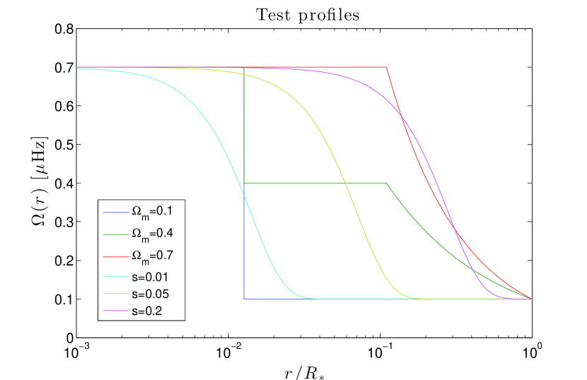
Figure 5: Synthetic rotation rate profiles used for testing. $\Omega_{m}$ refers to the rotation rate between 1.5 $r_{H}$ and the base convective zone, see Eq. 24. $s$ refers to the width of a Gaussian profile as defined in Eq. 26.

We compute the rotational splittings of the six test profiles using Eq. 1 for all the $l=1$ mode frequencies of the true model within $\pm 3\,\Delta\nu$ from the frequency at maximum power $\nu_{\mathrm{max}}$ . Then we compute the optimal combination of parameters $(q,\leavevmode\nobreak\ \Delta\Pi_{1},\leavevmode\nobreak\ \epsilon_{g},\leavevmode\nobreak\ d_{01})$ that best reproduces these model frequencies in order to estimate $\zeta_{\mathrm{as}}$. As explained in Section 2.1, we compute interpolated splittings $\delta_{\Delta P}$ to correspond with each period spacing $\Delta P$ as well as interpolated period spacings $\Delta P_{\nu}$ to correspond with each splitting $\delta$, see Fig. 6.

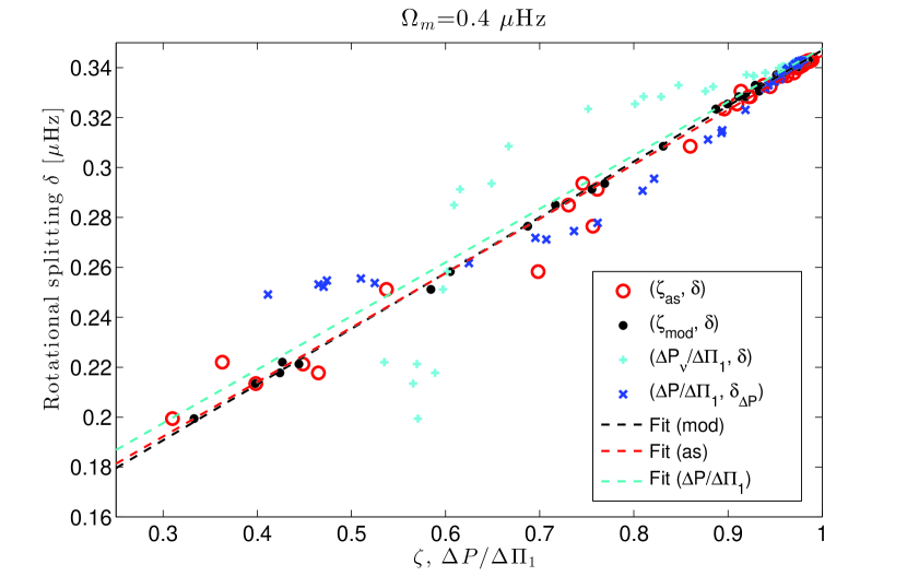
Figure 6: Rotational splittings using the best seismic model of KIC007619745 for one of the test profiles as defined in Eq. 24 with $\Omega_{c}=0.7\leavevmode\nobreak\ \mu$Hz, $\Omega_{m}=0.4\leavevmode\nobreak\ \mu$Hz, and $\Omega_{e}=0.1\leavevmode\nobreak\ \mu$Hz. The splittings $\delta_{\Delta P}$ (dark blue crosses) are the interpolated splittings as explained in Section 2.1. Dotted lines are linear fits providing estimates of the rotation rate averages in the g and p cavities following Eq. 3.

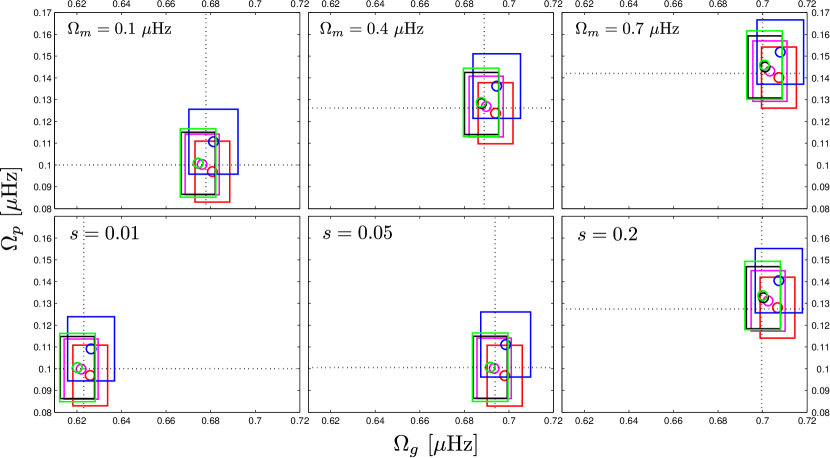
Figure 7: Comparison of the predicted rotation rate averages in the core ($\Omega_{g}$) and in the envelope ($\Omega_{p}$) using the methods described in Sections 2 and 3 based on the best seismic model for KIC007619745. The top row corresponds to rotation profiles following Eq. 24, and the bottom row corresponds to Gaussian rotation profiles according to Eq. 26. The black dashed lines mark the true averaged rotation rates as computed from Eqs. 4 and 5. Red represents the rotation rates as determined from linear fits of ($\zeta_{\mathrm{mod}},\,\delta$), and magenta represents the rotation rates from linear fits of ($\zeta_{\mathrm{as}},\,\delta$). Blue corresponds to linear fits of $\delta$ and $\delta_{\Delta P}$ vs $\Delta P_{\nu}/\Delta\Pi_{1}$ and $\Delta P/\Delta\Pi_{1}$. Black are the predictions from two-zone inversions, and green are the predictions from SOLA inversions. Results from Bayesian inference are not included here as they are essentially identical to the two-zone models.

Now we obtain the estimates of the rotation rates using each of the methods explained earlier. The true averages are obtained following Eqs. 4 and 5. In the case of the SOLA method, we computed the predicted rotation rates in two different locations: one at the surface of the star ($r/R_{*}=1$), and the other well within the radiative core ($r/R_{*}=10^{-3}$). These SOLA-predicted rotation rates are sensitive to the width $s$ of the target function. To obtain ‘calibrated’ values for $s,$ we therefore proceed first to compute the optimal two-zone model to determine the averages $\Omega_{g}$ and $\Omega_{p}$. Then we compute the rotational splittings associated with this two-zone model and use them as inputs for a SOLA inversion, adjusting the widths $s$ as necessary to make the corresponding SOLA predictions at $r/R_{*}=10^{-3}$ and $r/R_{*}=1$ exactly match $\Omega_{g}$ and $\Omega_{p}$, respectively. With the widths $s$ determined in this way, we then proceed to compute the SOLA-predicted averages using the splittings arising from the six test profiles.

We assume that the splittings all have the same uncorrelated Gaussian error distribution whose width matches the mean $1\sigma$ error from the actual measurements. In the case of the inversions, the corresponding uncertainties on the predicted rotation rates are computed via Eq. 19. In the case of the rotation rates estimated via linear fits involving $\zeta_{\mathrm{mod,\,as}}$ (see Fig. 6), the resulting uncertainties are computed through a Monte Carlo simulation sampling randomly and repeatedly for many times ($10^{5}$) from the normal distributions associated with each spliting $\delta$. For the fits of $\delta,\,\delta_{\Delta P}$ vs $\Delta P_{\nu}/\Delta\Pi_{1},\,\Delta P/\Delta\Pi_{1}$ we followed the same Monte Carlo approach, except that we also sampled randomly from the distributions associated each mode frequency $\nu,$ which we set as having the same standard deviation as the actual observed errors. We note that errors on the trapping parameter or systematic errors incurred by the inversions are not considered.

The predicted rotation rates are shown in Fig. 7. Although some scatter is present, the predictions are in acceptable agreement with the true averages across all methods. The test we just performed is an ideal situation, the modes are properly identified, the rotational kernels are based on the true seismic model, and the error distributions associated with the frequencies and splittings are centered exactly on the true values. Any deviation from this ideal situation will bring additional scatter to the predicted rotation averages.

The averaging kernels $\mathcal{K}(r)$ from the SOLA inversions at the two radial locations mentioned above, although well resolved with respect to each other, are essentially identical to the averaging kernels of the two-zone models at the corresponding zone, which suggests already that no more than two reasonably well-defined averages can be obtained using SOLA inversions.

Recently, Klion & Quataert (2016) proposed a method aiming to determine the region in a red giant star where differential rotation is concentrated. They note that the minimum normalized splitting, $\mathrm{min}(\delta/\mathrm{max}(\delta))$ can be used to distinguish between rotation profiles with differential rotation localized in the core from those with differential rotation localized mostly in the envelope. This is precisely the motivation of the functional form of the rotation profiles given by Eq. 24. For a fixed ratio $\Omega_{c}/\Omega_{e}$ in these profiles, the quantity $\mathrm{min}(\delta/\mathrm{max}(\delta))$ follows a one-to-one correspondence with $\Omega_{m}$ that determines the location of the differential rotation either in the core or in the envelope.

Di Mauro et al. (2016) were able to resolve three rotation rates in three distinct radial locations of KIC4448777, two of them within the radiative core, which allowed them to conclude that there is a steep gradient in the rotation there, thus localizing the differential rotation of the star inside the radiative core. The target in that study is very similar to the targets in our target selection, sharing similar evolutionary stages, therefore it may be possible in principle to resolve the rotation rate in at least two points inside the core. Unfortunately, the set of rotational kernels for all of our targets is not suitable for obtaining more than an averaged value across the core (see Fig. 11). The reason for this is not evident a priori, and although it deserves special attention, it is beyond the scope of the present study.

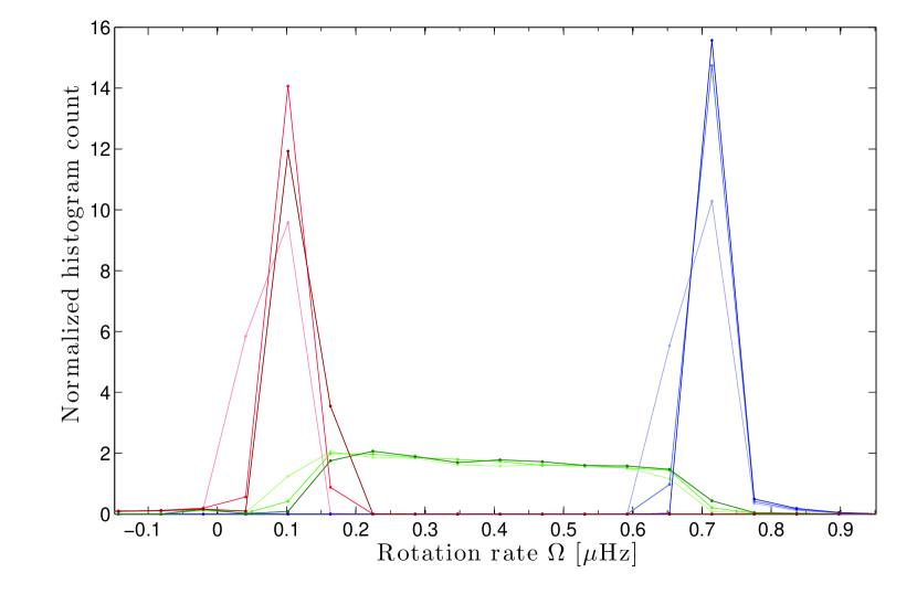
Figure 8: Histogram associated with the predictions for $\bar{\Omega}_{c,m,e}$ (blue, green, and red tones, respectively). The true (test) profile is described by Eq. 24 with fixed $\Omega_{c}=0.7\leavevmode\nobreak\ \mu$Hz, $\Omega_{e}=0.1\leavevmode\nobreak\ \mu$Hz. The light colors represent the histogram obtained when $\Omega_{m}=0.1\leavevmode\nobreak\ \mu$Hz, medium colors correspond to $\Omega_{m}=0.4\leavevmode\nobreak\ \mu$Hz, and dark colors represent $\Omega_{m}=0.7\leavevmode\nobreak\ \mu$Hz. Essentially identical distributions for $\bar{\Omega}_{m}$ result, regardless of the choice of $\Omega_{m}$. While $\Omega_{c}$ and $\Omega_{e}$ are recovered properly, no good prediction for $\Omega_{m}$ can be made.

We can use the idea by Klion & Quataert (2016) to determine whether we can indeed localize the differential rotation. We consider a rotation profile with some preestablished values for the set $(\Omega_{c},\Omega_{m},\Omega_{e})$ and compute its associated splittings. We consider splittings from all $l=1$ mixed modes within $\pm 3\,\Delta\nu$ of $\nu_{\mathrm{max}}$. With this set of splittings as input and considering errors on them matching the actual observed errors, we proceed to find the optimum combination of predicted $(\bar{\Omega}_{c},\bar{\Omega}_{m},\bar{\Omega}_{e})$ that minimizes the difference between the input and the predicted splittings. To minimize and obtain estimates of the three parameters, we use a downhill simplex method. Then we make use once again of a Monte Carlo simulation sampling randomly from the normal distributions associated with the input splittings to obtain distributions for $(\bar{\Omega}_{c},\bar{\Omega}_{m},\bar{\Omega}_{e})$. If enough information is indeed contained in the set of input splittings to constrain $\bar{\Omega}_{m}$, then this should reflect in a sharply peaked distribution for it. Figure 8 shows the results of this experiment. We set $\Omega_{c}=0.7\leavevmode\nobreak\ \mu$Hz, $\Omega_{e}=0.1\leavevmode\nobreak\ \mu$Hz, and vary $\Omega_{m}\in\{0.1,\leavevmode\nobreak\ 0.4,\leavevmode\nobreak\ 0.7\}\leavevmode\nobreak\ \mu$Hz. The predicted values for $\bar{\Omega}_{c}$ and $\bar{\Omega}_{e}$ are close to the true values, but the probability density distribution for $\bar{\Omega}_{m}$ is wide and practically flat, thus no reliable prediction for $\Omega_{m}$ is possible and the differential rotation cannot be localized properly. Essentially identical distributions of $\bar{\Omega}_{m}$ are obtained regardless of the choice of $\Omega_{m}$. This is a consequence of the magnitude of errors in the splittings together with the characteristics of the rotational kernels. Only if we artificially reduce the errors by an order of magnitude or less, a reasonable value of $\bar{\Omega}_{m}$ can be recovered. All of the 13 targets in our sample exhibit this undesirable behavior.

Table 1: Selected stellar parameters from observations and best seismic models. For each target, the top row contains observed quantities derived from Kepler data and bottom row contains quantities extracted from the best seismic model.

KIC id	$\Delta\nu$ ($\mu$Hz)	$\nu_{\mathrm{max}}$ ($\mu$Hz)	$\Delta\Pi_{1}$ (s)	$T_{\mathrm{eff}}$ (K)	[Fe/H]ini	$Y_{\mathrm{ini}}$	$f_{\mathrm{ov}}$ ($H_{P}$)	$M/M_{\odot}$	$R/R_{\odot}$
003744043	$9.90\pm 0.05$	$112.52\pm 0.25$	$76.0\pm 1.3$	$5112\pm 172$				$1.28\pm 0.18$
	$10.01$	112.84	75.64	5014	$-0.22$	0.300	0.0223	1.21	5.945
006144777	$11.01\pm 0.06$	$129.69\pm 0.24$	$79.3\pm 1.4$	$4746\pm 186$				$1.26\pm 0.18$
	$11.18$	130.92	79.63	4820	$0.02$	0.270	0.0353	1.15	5.431
007060732	$10.94\pm 0.05$	$132.29\pm 0.24$	$72.8\pm 1.4$	$4790\pm 164$				$1.33\pm 0.19$
	$11.04$	133.07	78.28	5056	$-0.22$	0.285	0.0190	1.37	5.821
007619745	$13.13\pm 0.07$	$170.82\pm 0.25$	$79.2\pm 1.3$	$5126\pm 169$				$1.58\pm 0.21$
	$13.28$	169.58	79.71	4969	$-0.10$	0.255	0.0183	1.34	5.122
008366239	$13.70\pm 0.07$	$185.56\pm 0.37$	$88.2\pm 1.3$	$5239\pm 170$				$1.76\pm 0.23$
	$13.74$	190.34	87.51	5142	$-0.22$	0.255	0.0043	1.71	5.419
008475025	$9.66\pm 0.05$	$112.95\pm 0.28$	$74.8\pm 1.4$	$5056\pm 154$				$1.46\pm 0.20$
	$9.72$	116.48	74.18	4751	$0.08$	0.240	0.0223	1.37	6.307
008718745	$11.40\pm 0.06$	$129.31\pm 0.25$	$79.4\pm 1.3$	$4825\pm 167$				$1.15\pm 0.16$
	$11.48$	139.33	80.70	4681	$0.14$	0.230	0.0249	1.15	5.308
009267654	$10.34\pm 0.05$	$118.63\pm 0.23$	$78.4\pm 1.4$	$5029\pm 156$				$1.37\pm 0.19$
	$10.41$	122.10	79.28	4794	$-0.04$	0.230	0.0391	1.20	5.759
010257278	$12.20\pm 0.06$	$149.47\pm 0.26$	$79.8\pm 1.4$	$5055\pm 152$				$1.50\pm 0.20$
	$12.28$	157.12	79.24	4981	$-0.16$	0.235	0.0195	1.44	5.517
011353313	$10.76\pm 0.05$	$126.46\pm 0.23$	$76.0\pm 1.4$	$5198\pm 168$				$1.48\pm 0.20$
	$10.97$	126.10	77.50	4941	$-0.16$	0.275	0.0145	1.16	5.558
011913545	$10.18\pm 0.05$	$117.16\pm 0.27$	$77.8\pm 1.3$	$4845\pm 145$				$1.37\pm 0.19$
	$10.27$	121.49	78.19	4637	$0.20$	0.230	0.0153	1.20	5.824
011968334	$11.41\pm 0.06$	$141.43\pm 0.26$	$78.1\pm 1.4$	$4914\pm 144$				$1.48\pm 0.20$
	$11.66$	135.35	78.60	4831	$-0.10$	0.235	0.0285	1.11	5.246
012008916	$12.90\pm 0.06$	$161.92\pm 0.31$	$80.5\pm 1.3$	$5002\pm 170$				$1.41\pm 0.19$
	$12.96$	169.60	79.79	4739	$0.20$	0.240	0.0197	1.33	5.168

5 Seismic modeling

From the original 19 young red giants studied by Corsaro et al. (2015), we selected only those stars that exhibit rotationally split dipole modes (triplets). In some cases, depending on the stellar inclination angle, some of the $l=1$ triplets were missing their central $m=0$ peaks although the split $m=\pm 1$ components were clearly visible. In these cases we assumed a central $m=0$ component in the middle of the observed $m=\pm 1$ frequencies, and we associated with it an error equal to three times the mean frequency error of the $l=0$ peaks (usually larger than the error on the $m=\pm 1$ components). This choice is conservative given that the asymmetry present in the full triplets (i.e., those that show central peaks) is usually smaller than this error. Assuming the presence of a central peak with this frequency uncertainty has virtually no effect on the uncertainty on the inferred rotation rates, given that in these cases the splittings are computed simply as half the distance in frequency of the $m=\pm 1$ components, without involving the hypothetical central component.

Equipped with these sets of pulsation frequencies, we set out to find approximate seismic models for each target making use of the MESA stellar evolution suite (Paxton et al., 2011, 2013, 2015) together with the GYRE pulsation code (Townsend & Teitler, 2013). The MESA suite includes the ‘astero’ module, which implements a downhill simplex search method (Nelder & Mead, 1965) to obtain the best stellar parameters given a set of pulsation and spectroscopic data. To reduce computing time during the search, we opted to include only the observed radial ($l=0$) modes and the dipole ($l=1$) modes. Including higher $l$ modes in the search, however desirable, would prohibitively increase the time required to find suitable seismic models for all targets.

Our approach consisted of a combination of grid and downhill simplex searches. We set up a grid of initial metallicities [Fe/H]_ini, varying from -0.22 to 0.2 with 0.06 steps (using a reference solar metallicity $Z_{\odot}/X_{\odot}$=0.02293 (Grevesse & Sauval, 1998)) and initial helium content $Y_{\mathrm{ini}}$ varying from 0.23 to 0.3 with 0.005 steps. For each pair ([Fe/H]_ini ,$Y_{\mathrm{ini}}$) we performed a downhill simplex search optimizing for initial mass and overshoot ($f_{\mathrm{ov}}$, expressed as a fraction of the pressure scale height $H_{P}$), in addition to age. We have kept the mixing length parameter $\alpha_{MLT}$ fixed at its solar calibrated value of 1.9. We also used Eddington-gray atmospheres and adopted the Asplund et al. (2009) mixture together with OPAL opacity tables (Iglesias & Rogers, 1996). When computing mode frequencies, we peformed atmospheric corrections following the method by Kjeldsen et al. (2008) using a calibrated value of the exponent $b=4.81$ as reported by Ball & Gizon (2014). The exact value of $b$ is not critical as the observed modes can still be identified one-to-one to model frequencies using slightly different values. Results are summarized in Table 1.

We performed a hare-and-hounds exercise to test our grid + downhill simplex approach. For this we extracted mode frequencies from the best model of KIC007619745, added some noise and used them as inputs to our search algorithm. The resulting model was satisfactorily close to the original, especially regarding the rotational kernels derived from them. We present more details in Appendix A.

$\begin{array}[]{cc}\includegraphics[width=195.12767pt]{KIC007619745_spdp1.eps}&\includegraphics[width=195.12767pt]{KIC007619745_spdp2.eps}\\ \includegraphics[width=195.12767pt]{hah_spdp1.eps}&\includegraphics[width=195.12767pt]{hah_spdp2.eps}\\ \end{array}$

Figure 9: Left column plots show the observed rotational splittings, normalized by their maximum value (red error bars) and the observed period spacings, normalized by the observed period spacing $\Delta\Pi_{1}$ (blue error bars) as functions of mode frequency for the target KIC 007619745 (top), and for the hare-and-hounds exercise. Right column plots show the observed rotational splitting $\delta$ as a function of $\zeta_{\mathrm{mod}}$ (red points and error bars), $\delta$ vs. $\zeta_{\mathrm{as}}$ (dark green points and error bars), and both $\delta$ vs. $\Delta P_{\nu}/\Delta\Pi_{1}$ and $\delta_{\Delta P}$ vs. $\Delta P/\Delta\Pi_{1}$ (blue points and cyan error bars). See Section 2.1.

6 Internal rotation rates

We estimated the internal rotation rates using two-zone models, Bayesian inference, and SOLA inversions (all based on the kernels provided by the seismic models) in addition to the model-independent method of Goupil et al. (2013) as described in Section 2. Figure 9 illustrates the use of the trapping parameter and associated linear fits as applied to the target KIC 007619745 as an example, as well as to the hare-and-hounds exercise explained in Appendix A.

We computed two-zone models with the inter-zone boundary in the middle of the evanescent zone for each target. For the SOLA inversions we set the trade-off parameter $\mu$ to zero since it made negligible difference on the results. In addition, for SOLA, we computed rotation rates at two radial locations, one at $r/R_{*}=10^{-3}$, deep in the radiative cores, and the other at the surface, $r/R_{*}=1$. The estimates of the rotation rates through SOLA do depend slightly on the width $s$ of the target functions used. To select the optimal value of $s,$ we took the two-zone rotation rates determined earlier and computed their associated splittings via Eq. 1. Then, using these synthetic splittings, we iteratively determined the optimal $s$ values required to exactly reproduce the two-zone rotation rates. With the widths $s$ thus determined, we then computed the rotation rates at $r/R_{*}=10^{-3}$ and at $r/R_{*}=1$ using the observed rotational splittings. The rotation rates estimated in this way are presented in Table 2 and in Figs. 15 and 16.

Table 2: Rotation rates in nHz estimated from two-zone models, SOLA inversions, Bayesian inference, linear fits of $\delta$ vs $\zeta_{\mathrm{mod}}$, linear fits of $\delta$ vs $\zeta_{\mathrm{as}}$, and linear fits of $\delta$ vs $\Delta P/\Delta\Pi_{1}$. For each target, the top row is the rotation rate of the core, and the bottom row is the rotation rate of the envelope. The four leftmost columns correspond to rotation rates based on seismic models, the next two columns present model-independent rotation averages. The last column presents an overall rotation rate computed as the mean from the six methods used; the corresponding overall error is computed by adding the mean variance to the inter-variance across the methods. See also Figs 15 and 16

KIC id	Two-zone	SOLA	Bayes	$\delta(\zeta_{\mathrm{mod}})$	$\delta(\zeta_{\mathrm{as}})$	$\delta(\Delta P/\Delta\Pi_{1})$	Overall
003744043	$541.8\pm 9.2$	$525.9\pm 15.6$	$544.8\pm 9.3$	$537.1\pm 16.0$	$536.9\pm 16.2$	$529.6\pm 17.9$	$536.0\pm 16.1$
	$75.8\pm 25.9$	$110.9\pm 29.8$	$72.6\pm 25.2$	$88.0\pm 28.2$	$78.9\pm 30.7$	$92.0\pm 32.2$	$86.4\pm 32.1$
006144777	$476.9\pm 2.9$	$458.6\pm 8.9$	$479.0\pm 2.7$	$470.5\pm 7.9$	$485.9\pm 5.8$	$485.3\pm 12.3$	$476.0\pm 12.7$
	$3.0\pm 10.4$	$73.2\pm 19.1$	$8.0\pm 8.0$	$48.3\pm 14.8$	$6.8\pm 16.2$	$26.5\pm 25.4$	$27.6\pm 32.6$
007060732	$629.0\pm 2.1$	$620.7\pm 15.1$	$633.0\pm 2.2$	$630.9\pm 12.6$	$649.6\pm 12.7$	$646.7\pm 20.1$	$635.0\pm 16.8$
	$66.1\pm 20.4$	$74.9\pm 39.4$	$64.1\pm 19.9$	$62.1\pm 35.2$	$4.6\pm 39.5$	$29.3\pm 39.9$	$50.2\pm 43.2$
007619745	$731.8\pm 12.8$	$733.3\pm 14.0$	$738.1\pm 13.0$	$740.0\pm 13.1$	$735.6\pm 12.8$	$745.2\pm 22.8$	$737.3\pm 16.0$
	$50.9\pm 16.1$	$48.1\pm 18.0$	$48.2\pm 15.8$	$46.5\pm 16.0$	$52.2\pm 15.5$	$45.8\pm 24.5$	$48.6\pm 18.1$
008366239	$434.3\pm 17.9$	$436.5\pm 19.3$	$439.1\pm 18.2$	$440.0\pm 18.3$	$461.5\pm 20.2$	$432.1\pm 28.4$	$440.6\pm 23.3$
	$80.1\pm 20.4$	$80.2\pm 22.6$	$79.6\pm 19.9$	$79.2\pm 20.0$	$36.7\pm 25.3$	$90.2\pm 23.5$	$74.3\pm 29.0$
008475025	$622.6\pm 0.5$	$607.4\pm 3.3$	$625.2\pm 0.5$	$617.9\pm 2.5$	$660.9\pm 2.4$	$622.7\pm 19.3$	$626.1\pm 19.9$
	$102.1\pm 1.2$	$130.3\pm 6.7$	$98.7\pm 1.1$	$115.5\pm 6.0$	$15.8\pm 6.8$	$76.4\pm 27.7$	$89.8\pm 42.3$
008718745	$813.7\pm 40.1$	$749.0\pm 37.7$	$816.7\pm 40.4$	$812.6\pm 40.7$	$853.7\pm 43.8$	$803.5\pm 41.7$	$808.2\pm 53.0$
	$131.9\pm 37.8$	$177.9\pm 44.9$	$128.3\pm 36.8$	$151.3\pm 39.2$	$36.4\pm 52.2$	$80.9\pm 52.5$	$117.8\pm 67.7$
009267654	$911.4\pm 0.8$	$908.2\pm 3.1$	$916.2\pm 0.8$	$915.3\pm 2.1$	$937.3\pm 2.4$	$939.4\pm 19.3$	$921.3\pm 15.8$
	$54.6\pm 5.4$	$65.0\pm 9.8$	$52.9\pm 5.3$	$57.9\pm 8.4$	$-23.1\pm 10.1$	$20.8\pm 21.8$	$38.0\pm 35.6$
010257278	$959.6\pm 33.6$	$930.6\pm 36.4$	$966.9\pm 34.0$	$969.0\pm 34.1$	$1024.2\pm 38.7$	$1002.3\pm 49.3$	$975.4\pm 50.4$
	$137.7\pm 49.0$	$188.3\pm 55.9$	$132.9\pm 48.0$	$131.8\pm 48.0$	$-1.5\pm 63.4$	$33.6\pm 64.9$	$103.8\pm 90.8$
011353313	$891.3\pm 23.0$	$901.2\pm 25.4$	$888.3\pm 21.5$	$901.1\pm 25.6$	$914.4\pm 26.9$	$908.2\pm 37.5$	$900.7\pm 28.9$
	$78.7\pm 27.5$	$88.9\pm 32.9$	$77.0\pm 26.2$	$86.5\pm 35.5$	$50.7\pm 40.4$	$77.6\pm 51.5$	$76.6\pm 39.1$
011913545	$559.1\pm 0.4$	$544.7\pm 2.6$	$559.2\pm 0.3$	$550.7\pm 2.2$	$566.1\pm 2.6$	$559.5\pm 11.6$	$556.5\pm 9.1$
	$-13.7\pm 2.5$	$53.1\pm 7.9$	$0.4\pm 0.4$	$45.3\pm 7.1$	$-3.9\pm 9.1$	$22.4\pm 14.0$	$17.3\pm 28.7$
011968334	$767.8\pm 9.9$	$727.8\pm 23.8$	$767.6\pm 9.9$	$729.5\pm 22.2$	$746.6\pm 21.6$	$743.0\pm 25.6$	$747.0\pm 26.5$
	$119.4\pm 15.2$	$73.6\pm 27.1$	$127.0\pm 14.2$	$74.2\pm 28.1$	$22.7\pm 36.1$	$49.0\pm 34.1$	$77.6\pm 48.4$
012008916	$815.5\pm 0.9$	$735.5\pm 4.2$	$822.0\pm 0.9$	$745.9\pm 3.7$	$776.7\pm 4.7$	$712.2\pm 16.1$	$767.9\pm 45.1$
	$10.4\pm 3.2$	$113.6\pm 7.2$	$10.1\pm 3.1$	$108.8\pm 6.2$	$45.4\pm 7.7$	$80.3\pm 15.1$	$61.5\pm 47.2$

We assume that the observational errors on the splittings and on the mode frequencies are normally distributed. Since in general, a given mode frequency has two period spacings associated with it and each period spacing is associated with two mode frequencies (and therefore two rotational splittings), we opted to take interpolated values as explained in Section 2.1. We performed linear fits to the resulting set to estimate the average rotation rates of the core $\Omega_{g}$ and the envelope $\Omega_{p}$ according to Eq. 3. A straightforward Monte Carlo approach using the observed rotational splittings and frequencies, together with their normally distributed errors, reveals a correlation between $\Omega_{g}$ and $\Omega_{p}$ that is a reflection of the fact that in Eq. 3 the slope and the intercept are not independent of each other. The rotation rates using this technique are shown in Figs. 15 and 16 in the Appendix B as a cloud of small violet circles, the blue box is centered on the mean, and its size corresponds to the 1$\sigma$ standard deviation of the points in the cloud.

Table 2 summarizes the rotation rates for all 13 targets obtained by all the methods described in this work.

7 Discussion

$\begin{array}[]{cc}\includegraphics[width=195.12767pt]{avk1.eps}&\includegraphics[width=195.12767pt]{avk2.eps}\\ \end{array}$

Figure 10: Averaging kernels $\mathcal{K}(r)$ for both SOLA inversions at $r/R_{*}=10^{-3}$, $r/R_{*}=1$ and a two-zone model with $x_{c}=0.1$ (from the best model of KIC007619745). The left panel shows the central region, and the right panel shows the surface region.

The rotation rates for most of the targets show good agreement, while a few present some scatter in the envelope averages. The rotation rates agree with each other within 2$\sigma$ except for one case (see further below).

There are minor differences in the ideal case of many exactly measured splittings and exact seismic models, as described in Section 4. The differences in this case are attributed to the different nature of the averages as computed from each method, for example, the averages as defined by Eqs. 4 and 5 are not exactly the same as the averages from Eq. 18, even if we had many kernels $K(r)$ at our disposal to have very well localized averaging kernels $\mathcal{K}(r^{\prime},r)$.

However, considering the scatter of the predicted averages, we can still constrain the rotation rates in our targets with an error of about $0.05\leavevmode\nobreak\ \mu$Hz except in a few cases. No more than two averages that are well resolved spatially could be obtained using inversions and the seismic models, which was our hope given the previous success reported by Di Mauro et al. (2016).

We have chosen one of the stars in the sample (KIC 007619745) as an illustrative case to explain why only two values could be obtained. In Fig. 10 we show the averaging kernels $\mathcal{K}(r)$ for the two-zone model (inner and outer zones) and SOLA (at $r/R_{*}=10^{-3}$ and $r/R_{*}=1$). According to Eq. 18, these are simply the weight functions involved in the average. They are localized (at least enough to resolve the core and the envelope), with the inner-zone kernel and the $r/R_{*}=10^{-3}$ SOLA kernel concentrating in approximately the same region in the stellar core. On the envelope, the outer-zone kernel and the $r/R_{*}=1$ SOLA kernel coincide roughly as well, while they oscillate rapidly around zero as the radius is varied in the core regions. These rapid oscillations around zero do not present a problem since we are only interested in the integrated averages. Indeed, as Fig. 11 shows, the cumulative integrals of the averaging kernels are fortunately insensitive to the rapid oscillations. The outer-zone and the $r/R_{*}=1$ SOLA cumulative kernels start growing only at around $r/R_{*}=0.2$, where the inner-zone and the $r/R_{*}=10^{-3}$ cumulative kernels have already reached unity. These properties allow us to estimate rotation rate averages of the core separately from the envelope. The inner zone averaging kernel in the SOLA inversions is basically the same when we use other radial locations well inside the radiative core, that is to say, we obtain the same average. As we approach the hydrogen burning region near $r/R_{*}=0.01,$ however, there is significant contamination from the outer regions of the star, as is shown in Fig. 11. All of our targets exhibit essentially identical behavior.

We note, however, that although the two-zone and SOLA kernels coincide for most targets, there were some instances where they differ slightly. In Fig. 12 we show an example illustrating this point. The two-zone kernels exhibit some leakage that leads to appreciable differences in the rotation averages when compared with the SOLA kernels, for instance. This is the case for targets KIC 011913545 and KIC 012008916.

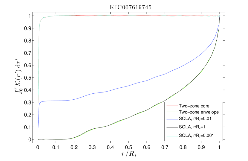
Figure 11: Cumulative integrals of the averaging kernels $\mathcal{K}(r)$ (from the best model of KIC007619745). The integrals corresponding to the inner two-zone model and SOLA at $r/R_{*}=10^{-3}$ are almost identical, the same holds for the outer two-zone and SOLA at $r/R_{*}=1$. A SOLA kernel at $r/R_{*}=0.01$ shows already significant leakage from other regions of the star, as shown by its cummulative integral not reaching unity anywhere close to that location.

$\begin{array}[]{cc}\includegraphics[width=195.12767pt]{good_kernel.eps}&\includegraphics[width=195.12767pt]{bad_kernel.eps}\\ \end{array}$

Figure 12: Cumulative integral of averaging kernels $\mathcal{K}(r)$ from SOLA inversions at $r/R_{*}=1$ (blue curves) and the cumulative integral from the outer two-zone model kernels (red curves). The left panel shows the case of KIC 008475025, where both cumulative integrals mostly coincide, are close to zero, and lead to similar average rotation rates of the envelope without appreciable leakage from central regions. In the case of KIC 011913545 (right panel) we see a difference between the cumulative integrals, particularly, the red curve is consistently below zero in the core region, which leads to leakage from these regions affecting the envelope averages.

The larger the number of splittings observed, the better the localization properties of the kernels will be and the error on the predicted rotation rates will be lower, see Fig.13. We note that the predicted errors as computed from Eq. 19 do not include any systematic errors arising from unmodeled physics, which means that the predicted rotation rates may be precise, but not accurate. This certainly constitutes a source for discrepancies in addition to the variability induced by poorly localized averaging kernels, as discussed above.

Accidental mode misidentification can potentially lead to an inadequate seismic model. As noted earlier, we are considering only modes with a detection probability higher than 0.99 (Corsaro et al., 2015). In principle, we therefore do not expect complications arising from this issue. Since a misidentified dipole mode might reveal itself as an outlier if its rotational splitting differs considerably from its prediction, we closely examined the rotational splittings of the star KIC 012008916 and compared them with the predicted two-zone model splittings. However, no particular mode stands out in a clear way. Still, we could prune out the modes whose splittings differ the most from the two-zone prediction. This exercise modifies the predicted rotation averages and removes the scatter bringing the predictions across the six methods in good agreement. This is still not satisfactory, however, since we have no means to a priori justify the adequacy of a two-zone rotation profile, or of any other particular profile, for that matter.

To conclude our discussion, we would like to point out that the target KIC 12008916 is coincidentally one of the few in the sample that has a very high inclination angle, that is, no central peaks were detected for it. This could be connected to the scatter in the rotation rates in some way.

$\begin{array}[]{cc}\includegraphics[width=390.25534pt]{error_test.eps}&\end{array}$

Figure 13: Error on the rotation averages using a synthetic rotation profile. Starting with the seismic model of KIC 012008916, we selected all the modes that had a trapping parameter $\zeta$ smaller than a particular cut-off. The total number of modes in the model is 45 (cutoff $\zeta=1$). We computed two-zone inversions using synthetic splittings from modes with trapping parameters smaller than a given $\zeta$ cutoff. More splittings used certainly improve the error on the predicted rotation averages, but this does not take into account any systematic errors that may be present.

8 Summary and conclusion

Building upon the mode-fitting and identification work of Corsaro et al. (2015), who analyzed the power spectra of 19 red giant targets recorded by the Kepler space telescope, we have estimated the average core and envelope rotation rate of 13 of these targets that showed clear rotationally split mixed modes. We employed the model-independent method developed originally by Goupil et al. (2013) and improved later by Deheuvels et al. (2015) and Mosser et al. (2015). This model-independent method aims to provide two rotational averages, one for the g-mode cavity and another for the p-mode cavity. To investigate the possibility of obtaining more detailed information about the rotation profile, we have used the traditional approach of searching for optimal seismic models with the aid of the MESA stellar evolution suite and the GYRE oscillation code.

We used a total of six different methods to compute the averages, four of them based on the optimal seismic models: SOLA inversions, two-zone inversions, Bayesian inference on two-zone models, and linear fits of the rotational splittings $\delta$ as functions of the trapping parameter $\zeta_{\mathrm{mod}}$. We also used the model-independent method as implemented by Deheuvels et al. (2015) and a variation of it based on the result by Mosser et al. (2015).

Before we applied these methods to our sample of red giants, we took a particular seismic model (that of KIC007619745) as a ‘true’ reference model, and in conjunction with six synthetic rotation profiles, we proceeded to compute the associated rotational splittings. Using these as inputs, we compared the predictions from all the methods against the ’true’ synthetic rotation profiles. We found good agreement in general, with some small differences that can be attributed to the slightly different nature of the averages produced by each method.

All the rotational kernels of our 13 targets allow the computation of two distinct rotation rates. We used the functional form of the rotation profiles used in the study by Klion & Quataert (2016) to test whether we could determine the approximate location in the star where the differential rotation takes place. The results were negative given the magnitude of the observational errors. The information contained in the splittings is insufficient to localize the region with differential rotation. This is perhaps closely related to the fact that no good averaging kernels could be found for intermediate regions of any of the targets.

The averages that we could obtain, however, are in good agreement with the average rotation rates of the g- and p-mode cavities as computed from the model-independent method for most of the targets, while a few targets present more scatter in the predicted averages across the different methods. The rotation rates agree with each other within 2$\sigma$ with only one exception, that of the star KIC 012008916. We identify the poorly localized two-zone averaging kernels as a contributor to the discrepancy. However, many sources of systematic errors exist that cannot be ruled out. There are indeed many simplifying assumptions involved in the stellar evolution code that directly affect the mode kernels, which means that some seismic models may not be adequate. In this respect, the model-independent methods are more reliable since they are essentially free of such systematic errors.

At any rate, the results for the rotation of the radiative cores show better agreement across all methods than the rotation of the envelopes, which is related to the fact that for p-dominated mixed modes the trapping parameter is $\zeta\approx 0.5$, far from $0$. The cores in this target selection are spinning about 5 to 10 times faster than their envelopes, which is consistent with previous studies and still calls for a better understanding of the angular momentum redistribution in stars in the red giant branch.

Appendix A Hare-and-hounds tests

The adequacy of the method we used to obtain the seismic models can be assessed by a hare-and-hounds exercise. First, we selected the best seismic model of KIC007619745 as our ‘true’ model, then we assumed a known internal rotation profile and derived ‘observations’ by adding some noise to the ‘true’ mode frequencies. The errors are assumed to be the same as in the actual observations. Then we used our grid + downhill simplex search strategy to obtain a seismic model that best reproduces these ‘observations’.

We have deliberately used a different mixing length parameter ($\alpha_{\mathrm{MLT}}=1.7$) and a different atmospheric correction power $b$ during the search ($b=4.9$) compared to the true model (which has $\alpha_{\mathrm{MLT}}=1.9$, $b=4.81$), thus further guaranteeing that the best model found is not identical to the true model. The best model properly recovers both the initial metallicity [Fe/H] and the initial helium content $Y$. The inferences on the internal rotation averages are also in good agreement with the true profile within $2\sigma$. However, the same cannot be said of other stellar parameters such as mass, $f_{\mathrm{ov}}$ , or radius.

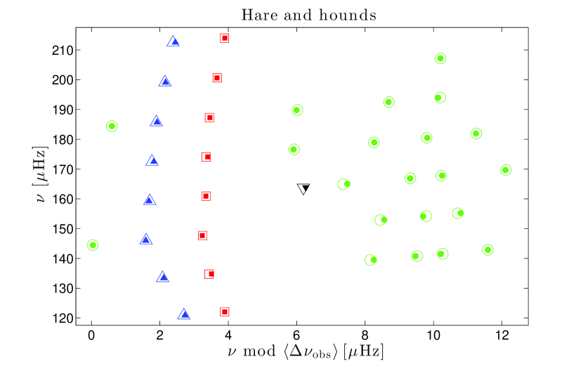
Figure 14: Échelle diagram comparing the noise-added true model frequencies (hollow symbols) and the best model found by a grid + simplex search approach (filled symbols). Red squares correspond to $l=0$ modes, green circles to $l=1$, blue triangles to $l=2,$ and inverted black triangles to $l=3$.

An échelle diagram comparing the frequencies of the best model with the noise-added true model is shown in Fig. 14. Table 3 lists other stellar parameters from the two models. The results for the internal rotation rates using different methods based on this best model are displayed in Fig. 16 (bottom, right panel). Here we used a ‘true’ rotation profile according to Eq. 24 with $\Omega_{c}=0.7\leavevmode\nobreak\ \mu$Hz, $\Omega_{m}=0.4\leavevmode\nobreak\ \mu$Hz, and $\Omega_{e}=0.1\mu\leavevmode\nobreak\$Hz. Compare also with the top and middle panel in Fig. 7.

Table 3: Hare-and-hounds model comparison

Model	$M/M_{\odot}$	$R/R_{\odot}$	$\Delta\nu$ [$\mu$Hz]	$T_{\mathrm{eff}}$ [K]	$f_{\mathrm{ov}}$
true	1.34	5.12	13.28	4969	0.0183
best	1.46	5.27	13.26	4872	0.0057

$\begin{array}[]{cc}\includegraphics[width=195.12767pt]{KIC003744043_omg3.eps}&\includegraphics[width=195.12767pt]{KIC006144777_omg3.eps}\\ \includegraphics[width=195.12767pt]{KIC007060732_omg3.eps}&\includegraphics[width=195.12767pt]{KIC007619745_omg3.eps}\\ \includegraphics[width=195.12767pt]{KIC008366239_omg3.eps}&\includegraphics[width=195.12767pt]{KIC008475025_omg3.eps}\\ \includegraphics[width=195.12767pt]{KIC008718745_omg3.eps}&\includegraphics[width=195.12767pt]{KIC009267654_omg3.eps}\\ \end{array}$

Figure 15: Rotation rates for all targets. Rotation rate of the envelopes ($\Omega_{p}$) on the ordinates, rotation rate of the cores ($\Omega_{g}$) on the abscissae. We show the results inferred from two-zone inversions (black), from SOLA inversions (green), from linear fits of $\delta$ vs. $\zeta_{\mathrm{mod}}$ (red), from linear fits of $\delta$ vs. $\zeta_{\mathrm{as}}$ (magenta), and from Bayesian inference (gray), all with their corresponding 1$\sigma$ error margins. The cloud of light blue circles is the result of applying linear fits of $\delta$ vs. $\delta P/\Delta\Pi_{1}$ sampling randomly from the splittings $\delta$ and the observed mode frequencies $\nu$, assuming a normal distribution for both. The blue error box indicates the $1\sigma$ standard deviation of the resulting distribution on each axis.

$\begin{array}[]{cc}\includegraphics[width=195.12767pt]{KIC010257278_omg3.eps}&\includegraphics[width=195.12767pt]{KIC011353313_omg3.eps}\\ \includegraphics[width=195.12767pt]{KIC011913545_omg3.eps}&\includegraphics[width=195.12767pt]{KIC011968334_omg3.eps}\\ \includegraphics[width=195.12767pt]{KIC012008916_omg3.eps}&\includegraphics[width=195.12767pt]{hah_omg3.eps}\\ \end{array}$

Figure 16: Continuation of Fig. 15. Rotation rate of the envelopes ($\Omega_{p}$) on the ordinates, rotation rate of the cores ($\Omega_{g}$) on the abscissae. We show the results inferred from two-zone inversions (black), from SOLA inversions (green), from linear fits of $\delta$ vs. $\zeta_{\mathrm{mod}}$ (red), from linear fits of $\delta$ vs. $\zeta_{\mathrm{as}}$ (magenta), and from Bayesian inference (gray), all with their corresponding 1$\sigma$ error margins. The cloud of light blue circles is the result of applying linear fits of $\delta$ vs. $\delta P/\Delta\Pi_{1}$ sampling randomly from the splittings $\delta$ and the observed mode frequencies $\nu$, assuming a normal distribution for both. The blue error box indicates the $1\sigma$ standard deviation of the resulting distribution on each axis.