When Does Diversity of User Preferences Improve Outcomes in Selfish Routing?

Abstract

We seek to understand when heterogeneity in user preferences yields improved outcomes in terms of overall cost. That this might be hoped for is based on the common belief that diversity is advantageous in many settings. We investigate this in the context of routing. Our main result is a sharp characterization of the network settings in which diversity always helps, versus those in which it is sometimes harmful.

Specifically, we consider routing games, where diversity arises in the way that users trade-off two criteria (such as time and money, or, in the case of stochastic delays, expectation and variance of delay). Our main contributions—a conceptual and a technical one— are the following:
1) A participant-oriented measure of cost in the presence of user diversity, together with the identification of the natural benchmark: the same cost measure for an appropriately defined average of the diversity.
2) A full characterization of those network topologies for which diversity always helps, for all latency functions and demands. For single-commodity routings, these are series-parallel graphs, while for multi-commodity routings, they are the newly-defined “block-matching” networks. The latter comprise a suitable interweaving of multiple series-parallel graphs each connecting a distinct source-sink pair.

While the result for the single-commodity case may seem intuitive in light of the well-known Braess paradox, the two problems are different: there are instances where diversity helps although the Braess paradox occurs, and vice-versa. But the main technical challenge is to establish the “only if” direction of the result for multi-commodity networks. This follows by constructing an instance where diversity hurts, and showing how to embed it in any network which is not block-matching, by carefully exploiting the way the simple source-sink paths of the commodities intersect in the “non-block-matching” portion of the network.

1 Introduction

People are inherently diverse and it is a common belief that diversity helps. In one of the central themes of algorithmic game theory—the tension between selfish behavior and social optimality—can diversity of user preferences help to bring us closer to the coveted social optimality? We provide an answer to this question in the context of non-atomic selfish routing, where diversity naturally arises in the way users trade-off two criteria, for example, time and money, or, in the presence of uncertain delays, expectation and variance of delay.

Diversity is reflected in combining the two criteria via different individual coefficients, which we call the ‘diversity parameters’. We consider a linear combination of the two criteria, as in the literature on tolls where users minimize travel time plus tolls, e.g., (Beckmann et al., 1956; Fleischer et al., 2004) or the literature on risk-averse selfish routing where users minimize expected travel time plus variance ((Nikolova and Stier-Moses, 2014)), or more generally travel time plus a deviation function ((Kleer and Schäfer, 2016)).

We are interested in understanding whether heterogeneity in user preferences improves collective outcomes or makes them worse. As we shall see, there is no unique answer. Rather, it depends on the setting. To address our question we need to specify how to measure the cost of an outcome, and define our comparison point, namely a benchmark setting with no user heterogeneity. As explained above, to measure the cost of an outcome, we treat a user’s cost as the sum of two terms associated with two criteria: If we let $\ell_{P}$ denote the cost of one criterion (e.g., the latency) over a path $P$, and $v_{P}$ be the cost of the second criterion, then the overall cost is given by $\ell_{P}+r\cdot v_{P}$, where $r$ is our diversity parameter. The special case of $r=0$ corresponds to indifference to the second criterion and results in the classic selfish routing model where users simply minimize travel time.

A first approach to measuring the effect of diversity might be to compare the cost of an outcome with $r=0$ (i.e., just the total latency) to that with other values of $r$, including possibly mixed values of $r$ across the population being routed. However, this approach does not pinpoint the gains and losses from user heterogeneity as opposed to user homogeneity; rather, it (mostly) pinpoints the gains and losses depending on whether players are affected by the second criterion or not. Instead, we focus on the sum of the costs incurred by the users as measured by their cost functions, and compare costs incurred by a heterogeneous population of users to those incurred by an equivalent population of homogeneous users. What are equivalent populations? Suppose the heterogeneous population’s diversity profile is given by a population density function $f(r)$. Then, we define the corresponding homogeneous population to have the single diversity parameter $\bar{r}=\int rf(r)dr$. In addition, we require the two populations to have the same size, in the sense that the total source-to-sink flows that they induce are equal.

For this setting, we completely characterize the graphs for which user heterogeneity does no harm, in the sense of only reducing the total cost as perceived by users, for both the case of a single commodity (i.e. one source-to-sink flow) and for multiple commodities (i.e. flows between multiple source-sink pairs). For the single-commodity case, these graphs are exactly the series-parallel graphs, with the source being the “start” vertex of the graph, and the sink being the “terminal” vertex. For the multi-commodity case, each commodity flows over a series-parallel graph, and further these subgraphs need to overlap in a particular manner which we specify later, in the formal statement of results. For all other graphs, we provide examples of desired source-to-sink demands for which the resulting equilibrium flows are more expensive than the flows in the corresponding homogeneous problem.

Related work. To the best of our knowledge this is the first work that methodically compares the effects of heterogeneity and homogeneity in user preferences for a self-interested routing population. In fact, in the broader area of algorithmic game theory, this seems to be the first time that a question of this type has been considered, with the exception of Chen et al. (2014). Algorithmic game theory research mentioning diversity exists in the context of the theory of evolution (e.g., Mehta et al. (2015); Chastain et al. (2013)), which is very different from our focus.

Since we provide attitudes to time versus money and time versus risk as motivating examples for user diversity, we briefly mention related work on tolls and on risk-averse selfish routing. Regarding the latter, there are multiple ways to model how the behavior of players incorporates risk when uncertainty is present (see e.g. Rockafellar (2007)). Piliouras et al. (2013) studied the effect that different risk attitudes may have on a system’s performance at equilibrium. They did so by examining the price of anarchy (i.e. the ratio of the cost at equilibrium to the optimal cost) for different risk formulations. Nikolova and Stier-Moses (2015) and Lianeas et al. (2016) studied the degradation of a network’s performance due to risk aversion. This kind of degradation is captured by the price of risk aversion, which compares the cost of the equilibrium when players are risk-averse to the equilibrium cost when players are risk-neutral. The above works assumed that all players have the same risk averse preferences, which we call risk homogeneity; they do not offer any indication as to whether and under what circumstances risk heterogeneity improves or harms a system’s performance. In contrast, Fotakis et al. (2015) considered games with heterogeneous risk-averse players. They showed how uncertainty may and can be used to improve a network’s performance, but the effects of heterogeneity as opposed to homogeneity were left unexamined. Regarding the related literature on tolls, early results (e.g., Beckmann et al. (1956)) showed that tolls can help implement the social optimum as an equilibrium, when users all have the same linear objective function combining time and money. Much more recently, these results were extended to the case where users trade-off travel time and money differently, by Cole et al. (2003) and Fleischer (2005) for the single commodity case, and by Karakostas and Kolliopoulos (2004b) and Fleischer et al. (2004) for the multicommodity case. We remark that in the above works, apart from Cole et al. (2003), the social welfare is defined as the total travel time, whereas in our work we consider the total user cost, which encapsulates both criteria. This, for example, is also the case for Christodoulou et al. (2014) and Karakostas and Kolliopoulos (2004a). We further note that if the social welfare is defined as the total travel time then there are simple instances on parallel link graphs where diversity is harmful.

Characterizing the topology of networks that satisfy some property is a common theme in computer science. Relevant to our work, Epstein et al. (2009) characterized the topology of single-commodity networks for which all Nash equilibria are social optima (under bottleneck costs), and Milchtaich (2006) characterized the topology of single-commodity networks which do not suffer from the Braess Paradox for any cost functions. Chen et al. (2015) fully characterized the topology of multi-commodity networks that do not suffer from the Braess paradox. These characterizations appear similar to ours, although there does not seem to be any other connection between the two problems, as (i) there are instances where diversity helps while the Braess Paradox occurs and others where diversity hurts but the paradox does not occur, and (ii) the Braess Paradox may occur in series-parallel networks when considering selfish routing with heterogeneity in user preferences, which is not the case for the classic selfish routing model.

In the following works, the characterizing topology for the corresponding question (for a single commodity) is similar to ours. Fotakis and Spirakis (2008) considered atomic games and proved that series-parallel networks are the largest class of networks for which strongly optimal tolls are known to exist. Nikolova and Stier-Moses (2015) considered homogeneous agents and a social cost function that does not account for the second criterion; They showed that series-parallel networks admit the best bound on the degradation of the network due to risk aversion. Theorem 4 of Acemoglu et al. (2016), proves that series-parallel networks are the characterizing topology for what they call the Informational Braess Paradox with Restricted Information Sets; this theorem compares the cost of one agent type before and after more information is revealed to agents of that type, but does not consider the change in the cost of other agent types. In contrast, our work considers non-atomic games with heterogeneous agents and bounds the overall costs faced by the collection of agents. Most relevant to our work is Meir and Parkes (2014) and its Theorem 3.1 as it implies that for series-parallel networks the cost of an agent of average parameter only increases when switching from the heterogeneous instance to the corresponding homogeneous one and thus for our sufficiency theorems, one is left to prove that the heterogeneous equilibrium cost is no greater than the cost of an agent of average parameter (though we give a different proof).

Contribution. We fully characterize the topology of networks for which diversity is never harmful, regardless of the demand size and the distribution of the diversity parameter (discrete or continuous). We do so both for single and multi-commodity networks.

For single-commodity networks it turns out that this topology is that of series-parallel networks. In Theorem 3.1, we show that if the network is series-parallel, then diversity only helps for any choice of demand and edge functions. The key observation is that there is a path for which the homogeneous flow is at least as large as the heterogeneous flow. As the cost of the homogeneous flow is the same on all used paths, while the cost of each unit of heterogeneous flow is lowest on the path it uses, one can then deduce that the cost of the heterogeneous flow is at most that of the homogeneous flow. To show necessity, we first provide an instance on the Braess graph for which diversity is harmful, and then show how to embed it in any non-series-parallel graph.

In multi-commodity networks, by the result above, each commodity must route its flow through a series-parallel subnetwork. But, as Proposition 2 shows, this is not enough, and the way in which these series-parallel networks overlap needs to be constrained. The necessary constraint is exactly captured by the class of block-matching networks, defined in this paper. Sufficiency in this case then follows quite easily from the same result for the single commodity case.

The main technical challenge is to show necessity. To this end, assuming diversity does no harm, we show, via a case analysis, how the subnetworks of the commodities may overlap. First, in Proposition 2, we give an instance on a network of two commodities and three paths for which diversity hurts. Then we mimic this instance on a general network. The difficult part is to choose the corresponding paths for the mimicking, so that, in the created instance, all the flow under both equilibria goes through these paths. The challenge is that the commodities’ subnetworks may overlap in subtle ways.

2 Preliminaries

We consider a directed multi-commodity network $G=(V,E)$ with an aggregate demand of $d_{k}$ units of flow between origin-destination pairs $(s_{k},t_{k})$ for $k\in K$. We let $\mathcal{P}_{k}$ be the set of all paths between $s_{k}$ and $t_{k}$, and $\mathcal{P}:=\cup_{k\in K}\mathcal{P}_{k}$ be the set of all origin-destination paths. We let $[m]$ denote $\{1,\ldots,m\}$. We assume that $K=[m]$, for some $m$. The users in the network—i.e., the players of the game—must choose routes that connect their origins to their destinations. We encode the collective decisions of users in a flow vector $f=(f_{\pi})_{\pi\in\mathcal{P}}\in\mathbb{R}^{|\mathcal{P}|}_{+}$ over all paths. Such a flow is feasible when demands are satisfied, as given by constraints $\sum_{\pi\in\mathcal{P}_{k}}f_{\pi}=d_{k}$ for all $k\in K$. For simplicity, we let $f_{e}$ denote the flow on edge $e$; note that $f_{e}=\sum_{\pi:e\in\pi}f_{\pi}$. When we need multiple flow variables, we use the analogous notation $g,g_{\pi},g_{e}$.

The network is subject to congestion that affects two criteria the players consider. These two criteria are modeled by two edge-dependent functions that take as input the edge flow $f_{e}$ of $e$, for each edge $e$: a latency function $\ell_{e}(x)$ assumed to be continuous and non-decreasing, and a deviation function $\sigma_{e}(x)$ assumed to be continuous (but not necessarily non-decreasing). Function $\ell_{e}(\cdot)$ represents the first criterion while $\sigma_{e}(\cdot)$ represents the second criterion.

Players choose paths according to a linear combination of the first criterion and the second criterion along the route. Throughout the paper we refer to the players’ objective as the cost along a route. Formally, for a given user, on letting $\ell_{\pi}(f)=\sum_{e\in\pi}{\ell_{e}(f_{e})}$ and $\sigma_{\pi}(f)=\sum_{e\in\pi}{\sigma_{e}(f_{e})}$, for a constant $r\geq 0$ that quantifies the user diversity parameter, the user’s cost along route $\pi$ under flow $f$ is

$$c^{r}_{\pi}(f)=\sum_{e\in\pi}{\ell_{e}(f_{e})}+r\sum_{e\in\pi}{\sigma_{e}(f_{e})}=\ell_{\pi}(f)+r\sigma_{\pi}(f)$$ (1)

We assume that for any edge and for any player’s diversity parameter $r$, the functions $\ell_{e}$ and $\ell_{e}+r\sigma_{e}$ are non-decreasing. We note that if there is an upper bound $r_{\max}$ on the possible values of the diversity parameter $r$, then the latter assumptions do not require $\sigma_{e}$ to be non-decreasing. This is desirable because, for example, in risk-averse selfish routing where $\sigma_{e}$ models the variance, $\sigma_{e}$ can be a decreasing function of the flow.

Players Heterogeneity. We assume that the diversity parameter distribution $r_{k}$ for each commodity $k$ is heterogeneous, i.e. there may be more than one value of the diversity parameters $r$ for the players routing commodity $k$. We use the term single-minded to refer to players with $r=0$.

We consider two cases: where the distribution of the diversity parameter among the players is discrete and where it is continuous. For a discrete distribution of, say, $n$ discrete values $r^{k}_{1},\ldots,r^{k}_{n}$, the demand $d_{k}$ is a vector $d_{k}=(d^{k}_{1},\ldots d_{n}^{k})$ where each $d^{k}_{i}$ denotes the total demand of Commodity $k$ with diversity parameter $r^{k}_{i}$. We let $d^{k}$ denote Commodity $k$’s total demand, $d^{k}=\sum_{i=1}^{n}d^{k}_{i}$. For a continuous distribution with infimum and supremum $r^{k}_{\min}$ and $r^{k}_{\max}$ respectively, the demand $d_{k}$ is given by a density function $\rho_{k}:[r_{\min},r_{\max}]\rightarrow\mathbb{R}_{\geq 0}$ such that for any two values $r_{1}\leq r_{2}$ the total demand with diversity parameter $r_{1}\leq r\leq r_{2}$ has magnitude $\int_{r_{1}}^{r_{2}}\rho_{k}(r)dr$, and ${d^{k}}=\int_{r^{k}_{\min}}^{r^{k}_{\max}}\rho_{k}(r)dr$. Variables $f^{r}_{\pi}$ and $f_{e}^{r}$ denote the flow of diversity parameter $r$ on path $\pi$ and edge $e$, respectively.

Formally, an instance is described by the tuple $(G,\{(\ell_{e},\sigma_{e})\}_{e\in E},\{(s_{k},t_{k})\}_{k\in K},\{d_{k}\}_{k\in K},\{r_{k}\}_{k\in K})$ for the discrete case, where $r_{k}=(r^{k}_{1},\ldots,r^{k}_{n})$ is the vector of different diversity parameters encountered in the heterogeneous population, and by the tuple $(G,\{(\ell_{e},\sigma_{e})\}_{e\in E},\{(s_{k},t_{k})\}_{k\in K},\{\rho_{k}\}_{k\in K})$ in the continuous case.

Equilibrium flows. The Wardrop equilibrium of an instance is a flow $f$ such that for every $k\in K$, for every path $\pi\in\mathcal{P}_{k}$ with positive flow, and any diversity parameter $r$ on it, the path cost $c_{\pi}^{r}(f)\leq c_{\pi^{\prime}}^{r}(f)$ for all paths $\pi^{\prime}\in\mathcal{P}_{k}\,$.

From here on, we shall refer to the Wardrop equilibrium as the equilibrium. Our goal is to compare the total user cost at the equilibrium of an instance with a population that has heterogeneous diversity parameters, to the total user cost at the equilibrium of the same instance but with the population of each commodity keeping its magnitude changed to be homogeneous, with diversity parameter equal to the expected value of the diversity parameter distribution in the heterogeneous population of the commodity. To differentiate more easily, for a heterogeneous instance we call the former the heterogeneous equilibrium and the latter the (corresponding) homogeneous equilibrium. We usually denote the heterogeneous equilibrium by $g$ and the homogeneous equilibrium by $f$. The existence of both equilibria is guaranteed by e.g. Schmeidler (1973, Theorem 2). We note here that in general we do not need uniqueness of equilibria, neither for the edge costs nor for the edge flows. Our results hold for any arbitrary pair of heterogeneous and homogeneous equilibria of the corresponding instances. Also, as for classic routing games, without loss of generality (WLOG) we may assume that equilibrium flows are acyclic.

Total Costs. For a heterogeneous equilibrium flow vector $g$, in the discrete case, the heterogeneous total cost of Commodity $k$ is denoted by $C^{k,ht}(g)=\sum_{j=1\ldots n}d^{k}_{j}c^{k,r_{j}^{k}}(g)$ where $c^{k,r_{j}^{k}}(g)$ denotes the common cost at equilibrium $g$ for players of diversity parameter $r_{j}^{k}$ in Commodity $k$. In the continuous case, the heterogeneous total cost of Commodity $k$ is denoted by $C^{k,ht}(g)=\int_{r^{k}_{\min}}^{r^{k}_{\max}}\rho_{k}(r)c^{k,r}(g)dr$, where $c^{k,r}(g)$ denotes the common cost at equilibrium $g$ for players of diversity parameter $r$ in Commodity $k$. The heterogeneous total cost of $g$ is then $C^{ht}(g)=\sum_{k\in K}C^{k,ht}(g)$. For the corresponding homogeneous equilibrium flow $f$, i.e. the instance with diversity parameter $\bar{r}^{k}$, where $\bar{r}^{k}$ denotes the average diversity parameter for Commodity $k$, players of Commodity $k$ share the same cost $c^{\bar{r}^{k}}(f)$. Then, the homogeneous total cost of Commodity $k$ under $f$ is $C^{k,hm}(f)=d_{k}c^{\bar{r}^{k}}(f)$, and the homogeneous total cost of $f$ is $C^{hm}(f)=\sum_{k\in K}C^{k,hm}(f)$. Finally, if $C^{ht}(g)\leq C^{hm}(f)$, we say that diversity helps; if not, we say that diversity hurts. For our characterization to be meaningful, we assume an average-respecting demand, i.e., a demand where $\forall i,j:\bar{r}^{i}=\bar{r}_{j}$. Otherwise, diversity may hurt in simple instances, e.g., with two parallel links and two commodities (see Appendix 0.A.1 for an example).

Networks. For a network $G$ we let $V(G)$ and $E(G)$ denote its vertex set and edge set, respectively.

A directed $s\mbox{--}t$ network $G$ is series-parallel if it consists of a single edge $(s,t)$, or it is formed by the series or parallel composition of two series-parallel networks with terminals $(s_{1},t_{1})$ and $(s_{2},t_{2})$, respectively. In a series composition, $t_{1}$ is identified with $s_{2}$, $s_{1}$ becomes $s$, and $t_{2}$ becomes $t$. In a parallel composition, $s_{1}$ is identified with $s_{2}$ and becomes $s$, and $t_{1}$ is identified with $t_{2}$ and becomes $t$. The internal vertices of a series-parallel network $G$ are all its vertices other than its terminals.

An $s\mbox{--}t$ series-parallel network may be represented using a sequence of networks $B_{j}$ connected in series, where each $B_{j}$ is either a single edge or two series-parallel networks connected in parallel. Given a series-parallel network $H$, we can write $H=sB_{1}v_{1}B_{2}v_{2}\ldots B_{b-1}v_{b-1}B_{b}t$, where for any $j$ and triple $xB_{j}y$, $x$ and $y$ are the terminals of the series-parallel network $B_{j}$, and $B_{j}$ is either a single edge or a parallel combination of two series-parallel networks. We refer to the $B_{j}$’s as blocks, the prescribed representation as the block representation of $H$, and the $v_{i}$’s as separators, as they separate $s$ from $t$. Two series-parallel networks $G_{1}$ and $G_{2}$ are said to be block-matching if for every block $B$ of $G_{1}$ and every block $D$ of $G_{2}$, either $E(B)=E(D)$ or $E(B)\cap E(D)=\emptyset$. Note that $E(B)=E(D)$ implies that $B$ and $D$ have the same terminals and direction, as for either $B$ or $D$, the source vertex will have only outgoing edges toward the internal vertices and the target vertex will have only incoming edges from the internal vertices.

For a $k$-commodity network $G$, let $G_{i}$ be the subnetwork of $G$ that contains all the vertices and edges of $G$ that belong to a simple $s_{i}\mbox{--}t_{i}$ path for Commodity $i$. In other words, $G_{i}$ is the subnetwork of $G$ for Commodity $i$ that equilibria flows will consider, as they are, WLOG, acyclic. A multi-commodity network $G$ is block-matching if for every $i$, $G_{i}$ is series-parallel, and for every $i,j$, $G_{i}$ and $G_{j}$ are block-matching. An example is given in Figure 1.

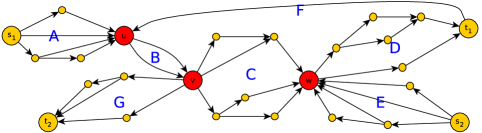
Figure 1: A block-matching network of $2$ commodities. $G_{1}$ and $G_{2}$ are series-parallel and their block representations are $G_{1}=s_{1}AuBvCwDt_{1}$ and $G_{2}=s_{2}EwDt_{1}FuBvGt_{2}$. $G_{1}$ and $G_{2}$ share exactly blocks $B$ and $D$ and do not share any edge on any other of their blocks. If we add an edge from $s_{1}$ to $t_{1}$, then the network stops being block-matching since $G_{1}$ will be a block by itself and it will not match any of the blocks of $G_{2}$.

3 Topology of Single-Commodity Networks for which Diversity Helps

In this section, we fully characterize the topology of single-commodity networks for which, with any choice of heterogeneous demand and edge functions, diversity helps. WLOG we may restrict our attention to single-commodity networks whose edges all belong to some simple source-destination path as only these edges are going to be used by the (WLOG, acyclic) equilibria and thus all other edges can be discarded. It turns out that this topology is exactly that of series-parallel networks (Theorems 3.1 and 3.2). Ommited proofs can be found in Appendix 0.A.

3.1 Series Parallel Implies Diversity is Helpful

Throughout this section we will be considering a heterogeneous instance $\mathcal{G}$ on an $s\mbox{--}t$ series-parallel network $G$. We let $\mathcal{F}$ denote the corresponding homogeneous instance. We let $g$ denote an equilibrium flow for $\mathcal{G}$ and $f$ an equilibrium flow for $\mathcal{F}$. Finally, we let $C^{ht}(g)$ denote the cost of flow $g$ and $C^{hm}(f)$ the cost of flow $f$. Although redundant, we keep the superscripts as a further reminder of the flow type at hand.

The key observation is that there is a path $P$ used by flow $f$ such that for every edge in $P$, $f_{e}\geq g_{e}$, and hence for any $r\in[0,r_{\max}]$, $c_{p}^{r}(f)\geq c_{p}^{r}(g)$ (Lemmas 1 and 2). We then deduce our result: $C^{ht}(g)\leq C^{hm}(f)$ (Theorem 3.1).

Lemma 1

Let G be an $s\mbox{--}t$ series-parallel network and let $x$ and $y$ be flows on $G$ that route $d_{1}$ and $d_{2}$ units of traffic respectively, with $d_{1}\geq d_{2}$ and $d_{1}>0$. Then, there exists an $s\mbox{--}t$ path $P$ such that for all $e\in P,x_{e}>0$ and $x_{e}\geq y_{e}$.

Lemma 2

There exists a path $P$ used by $f$ such that for any $r\in[0,r_{\max}]$, $c^{r}_{p}(g)\leq c^{r}_{p}(f)$.

Proof

Flows $f$ and $g$ have the same magnitude on the series-parallel network $G$. Applying Lemma 1 with $x=f$ and $y=g$ implies that there exists an $s\mbox{--}t$ path $P$ such that for all $e\in P,$ $f_{e}>0$, implying that WLOG $P$ is used by $f$, and $f_{e}\geq g_{e}$. By assumption, for any $r\in[0,r_{\max}]$, $\ell_{e}+r\sigma_{e}$ is non-decreasing, and thus for all $e\in P,\ell_{e}(f_{e})+r\sigma_{e}(f_{e})\geq\ell_{e}(g_{e})+r\sigma_{e}(g_{e})$. Consequently, $\sum_{e\in P}\big{(}\ell_{e}(f_{e})+r\sigma_{e}(f_{e})\big{)}\geq\sum_{e\in P}\big{(}\ell_{e}(g_{e})+r\sigma_{e}(g_{e})\big{)}\Leftrightarrow c^{r}_{p}(g)\leq c^{r}_{p}(f)$ as needed.

Theorem 3.1

$C^{ht}(g)\leq C^{hm}(f).$

Proof

Since $G$ is a series-parallel network, on setting $\bar{r}=E[r]$ and then applying Lemma 2, we obtain that there is a path $P$ used by $f$ such that

$$\ell_{p}(f)+\bar{r}\sigma_{p}(f)\geq\ell_{p}(g)+\bar{r}\sigma_{p}(g)$$ (2)

WLOG we can assume that the total demand $d=1$. We first bound the total cost of $g$ in terms of the cost of path $P$ under $g$ and then we use (2) to further bound it in terms of the cost of path $P$ under $f$. The latter equals the cost of $f$, as the demand is equal to $1$.

Consider the heterogeneous equilibrium flow $g$. By the equilibrium conditions, for any player of diversity parameter $r$, for any $r$, the cost she incurs with flow $g$ is $c^{r}(g)\leq\sum_{e\in p}{\ell_{e}(g_{e})}+r\sum_{e\in p}{\sigma_{e}(g_{e})}$. In other words, there is no incentive to deviate to path $P$ (if not already on it). Thus, if the diversity parameters are discrete, given by a demand vector $(d_{1},\ldots,d_{k})$ of diversity parameters $(r_{1},\ldots,r_{k})$,

$$C^{ht}(g)\leq\sum_{i=1\ldots k}d_{i}\Big{(}\sum_{e\in p}{\ell_{e}(g_{e})}+r_{i}\sum_{e\in p}{\sigma_{e}(g_{e})}\Big{)}=\ell_{p}(g)+\bar{r}\sigma_{p}(g),$$

with the last equality following as the total demand is 1 and the average diversity parameter is $\bar{r}=\sum_{i=1}^{k}d_{i}r_{i}$. If instead the diversity parameters are continuously distributed on the demand with density function $\rho(r)$, with $r_{\min}$ and $r_{\max}$ being their infimum and supremum respectively,

$$C^{ht}(g)\leq\int_{r_{\min}}^{r_{\max}}\rho(r)\Big{(}\sum_{e\in p}{\ell_{e}(g_{e})}+r\sum_{e\in p}{\sigma_{e}(g_{e})}\Big{)}dr=\ell_{p}(g)+\bar{r}\sigma_{p}(g),$$

with the last equality following as the total demand is 1, i.e. $\int_{r_{\min}}^{r_{\max}}\rho(r)dr=1$, and the average diversity parameter is $\bar{r}=\int_{r_{\min}}^{r_{\max}}r\rho(r)dr$. In both the discrete and continuous case, as $P$ is used by $f$, we have $C^{hm}(f)=\ell_{p}(f)+\bar{r}\sigma_{p}(f)$, and applying (2) we obtain

$$C^{ht}(g)\leq\ell_{p}(g)+\bar{r}\sigma_{p}(g)\leq\ell_{p}(f)+\bar{r}\sigma_{p}(f)=C^{hm}(f).$$

3.2 The Series Parallel Condition is Necessary

To prove the necessity of the network being series-parallel, we begin by constructing an instance for which diversity hurts, i.e. the heterogeneous equilibrium has total cost strictly greater than the total cost of the homogeneous equilibrium (Proposition 1). Then, in Theorem 3.2, we show how to embed this instance into any network that is not series-parallel.

Recall the Braess graph $G_{B}$, shown in Figure 2.

Proposition 1

For any strictly heterogeneous demand on the Braess graph $G_{B}$, there exist edge functions $(\ell_{e})_{e\in E}$ and $(\sigma_{e})_{e\in E}$ that depend on the demand, for which $C^{ht}(g)>C^{hm}(f)$. In addition, this remains true if we are restricted to only using affine functions.

Proof

We may assume WLOG that the demand is of unit size.

Let $\bar{r}$ be the average diversity parameter and let $r_{\min}$ be the infimum of the diversity parameters’ distribution. Let $r_{0}$ be any diversity parameter and let $d_{0}$ be the total demand with diversity parameter $\leq r_{0}$. Suppose that in addition, $r_{\min}\leq r_{0}<\bar{r}$, and the corresponding $d_{0}$ satisfies $d_{0}>0$. As the demand is strictly heterogeneous, there must be such an $r_{0}$. Later on, $r_{0}$ will be specified further.

In addition, we let $h$ be any continuous, strictly increasing cost function with $h(\frac{1}{2})=1$ and $h(\frac{1}{2}+\frac{d_{0}}{2})=1+\frac{\bar{r}-r_{0}}{2}$.

Consider the Braess graph $G_{B}=(\{s,u,v,t\},\{(s,u),(u,t),(u,v),(s,v),(v,t)\})$ with cost functions $\ell_{(s,u)}(x)=\ell_{(v,t)}(x)=h(x)$, $\sigma_{(s,u)}(x)=\sigma_{(v,t)}(x)=0$, $\ell_{(u,t)}(x)=\ell_{(s,v)}(x)=2+\frac{\bar{r}+r_{0}}{2}$, and $\sigma_{(u,t)}(x)=\sigma_{(s,v)}(x)=0$, and $\ell_{(u,v)}(x)=1$ and $\sigma_{(u,v)}(x)=1$. The instance is shown in Figure 2.

Figure 2: The Braess network with the edge functions of Proposition 1. The pair $a(x),b(x)$ on each edge denotes the latency and deviation functions, respectively.

The heterogeneous equilibrium $g$ routes $d_{0}$ units of flow through the zig-zag path, i.e.  path $s,u,v,t$; the rest of the flow is split between the upper and lower paths $s,u,t$ and $s,v,t$. This follows because with this routing, for players of diversity parameter $r\leq r_{0}$, the zig-zag path costs $2(1+\frac{\bar{r}-r_{0}}{2})+1+r\leq 2(1+\frac{\bar{r}-r_{0}}{2})+1+r_{0}=3+\bar{r}$ while the other paths cost $1+\frac{\bar{r}-r_{0}}{2}+2+\frac{\bar{r}+r_{0}}{2}=3+\bar{r}$, and for a player of diversity parameter $r\geq r_{0}$, the upper and lower paths cost $1+\frac{\bar{r}-r_{0}}{2}+2+\frac{\bar{r}+r_{0}}{2}=3+\bar{r}$ while the zig-zag path costs $2(1+\frac{\bar{r}-r_{0}}{2})+1+r\geq 2(1+\frac{\bar{r}-r_{0}}{2})+1+r_{0}=3+\bar{r}$.

To compute $C^{ht}(g)$, first note that players of diversity parameter $r>r_{0}$, who have total demand equal to $1-d_{0}$, have cost $3+\bar{r}$, and all players of any diversity parameter $r\leq r_{0}$ have cost $2(1+\frac{\bar{r}-r_{0}}{2})+1+r\geq 2(1+\frac{\bar{r}-r_{0}}{2})+1+r_{\min}=3+\bar{r}+r_{\min}-r_{0}$. The total cost of $g$ is thus $C^{ht}(g)\geq d_{0}(3+\bar{r}+r_{\min}-r_{0})+(1-d_{0})(3+\bar{r})=3+\bar{r}+d_{0}(r_{\min}-r_{0})$.

The homogeneous equilibrium $f$ uses only the upper and lower paths. This follows because with this routing, for the average diversity parameter, the upper and lower paths cost $1+2+\frac{\bar{r}+r_{0}}{2}=3+\frac{\bar{r}+r_{0}}{2}$, while the zig-zag path costs $1+1+\bar{r}+1=3+\bar{r}>3+\frac{\bar{r}+r_{0}}{2}$. The total cost of $f$ is thus $C^{hm}(f)=3+\frac{\bar{r}+r_{0}}{2}$.

Now we further specify $r_{0}$ so as to ensure $C^{ht}(g)>C^{hm}(f)$. By the above computations, it suffices to prove the existence of an $r_{0}$ that satisfies $r_{\min}\leq r_{0}<\bar{r}$ and $d_{0}>0$ and in addition satisfies

$$3+\bar{r}+d_{0}(r_{\min}-r_{0})>3+\frac{\bar{r}+r_{0}}{2}\Longleftrightarrow\frac{\bar{r}-r_{0}}{2}+d_{0}(r_{\min}-r_{0})>0.$$

As $r_{0}$ (which is $<\bar{r}$) goes to $r_{\min}$, the strictly positive quantity $\frac{\bar{r}-r_{0}}{2}$ increases and the non-positive quantity $d_{0}(r_{\min}-r_{0})$ goes to $0$ (because $d_{0}$ decreases and $r_{0}$ goes to $r_{\min}$). On the other hand, by definition, $r_{\min}$ is the infimum of the diversity parameters, and thus for any $\epsilon>0$, there is a positive demand with diversity parameter $r\leq r_{\min}+\epsilon$. Therefore, there exists an $r_{0}$ satisfying the above inequality with $r_{\min}\leq r_{0}<\bar{r}$ and $d_{0}>0$, as needed.

The above construction can be extended to only use affine functions. This can be done for example by changing function $h$ to the linear function that satisfies $h(0)=0$, $h(\frac{1}{2})=A$ and $h(\frac{1}{2}+\frac{d_{0}}{2})=A+\frac{\bar{r}-r_{0}}{2}$, and for that $A$ (in fact, $A=\frac{\bar{r}-r_{0}}{2d_{0}}$), only changing $\ell_{(s,v)}$, $\ell_{(u,t)}$ and $\ell_{(u,v)}$ to $\ell_{(s,v)}(x)=\ell_{(u,t)}(x)=2A+\frac{\bar{r}+r_{0}}{2}$ and $\ell_{(u,v)}(x)=A$.

Theorem 3.2

If $G$ is not series-parallel, then for any strictly heterogeneous demand there are cost functions for which $C^{ht}(g)>C^{hm}(f)$.

We defer the proof to the appendix. Instead, in the next section, we will enter into the more challenging construction needed for the multi-commodity case.

4 Topology of Multi-Commodity Networks for which Diversity Helps

In this section we fully characterize the topology of multi-commodity networks for which, with any choice of heterogeneous average-respecting demand and edge functions, diversity helps. Because of Theorem 3.2, if we require diversity to help on any instance on $G$, then for any commodity $i$, $G_{i}$ needs to be series-parallel. Yet, as we shall see in Proposition 2, this is not enough. We also need to understand the overlaps of the $G_{i}$’s. It turns out that the allowable overlaps are exactly captured by the topology of block-matching networks (Theorems 4.1 and 4.2). Ommited proofs can be found in Appendix 0.A.

4.1 Sufficiency

Using Theorem 3.1, we can obtain an analogous theorem for the multi-commodity case.

Theorem 4.1

Let $G$ be a $k$-commodity block-matching network. Then, for any instance on $G$ with average-respecting demand $C^{ht}(g)\leq C^{hm}(f).$

Proof

Consider Commodity $i$ and let $G_{i}=s_{i}B_{1}v_{1}\ldots v_{b_{i}-1}B_{b_{i}}t_{i}$ be its block representation. Consider an arbitrary $B_{j}$ with terminals $v_{j-1}$ and $v_{j}$. Because $G$ is block-matching, any other Commodity $l$ either contains $B_{j}$ as a block in its block representation or contains none of its edges. Also, recall that, as explained in the preliminaries section, if $G_{l}$ contains $B_{j}$, it has the same terminals $v_{j-1}$ and $v_{j}$. This implies that under any routing of the demand, either all of $l$’s demand goes through $B_{j}$ or none of it does. This means that under both equilibria $g$ and $f$, the total traffic routed from $v_{j-1}$ to $v_{j}$ through $B_{j}$ is the same which further implies that, if restricted to the block, the cost of the heterogeneous equilibrium is less than or equal to that of the homogeneous equilibrium: $C^{ht}(g)\Big{|}_{B_{j}}\leq C^{hm}(f)\Big{|}_{B_{j}}$. For the latter, recall that the demand is average-respecting and thus $f$ has a single average parameter. On the other hand, if we let $\mathcal{B}$ be the set of all the blocks of all commodities, then $C^{ht}(g)=\sum_{B\in{\mathcal{B}}}C^{ht}(g)\Big{|}_{B}$ and $C^{hm}(f)=\sum_{B\in{\mathcal{B}}}C^{hm}(f)\Big{|}_{B}$ which using the previous inequality proves the result.

4.2 Necessity

To derive the necessity we first give an example of a non-block-matching network for which diversity hurts (Proposition 2). Then, after proving some properties for commodities for which the corresponding $G_{i}$ are series-parallel (Lemmas 3 and 4), we mimic the above example to obtain contradicting instances for networks that are not block-matching and thereby prove Theorem 4.2.

Let $G$ be the following 2-commodity network, depicted in Figure 3. $G_{2}$, the subnetwork for Commodity 2, consists of a simple $s_{2}\mbox{--}t_{2}$ path $P_{2}$, while $G_{1}$, the subnetwork for Commodity 1, is formed from two simple $s_{1}\mbox{--}t_{1}$ paths named $P_{1}$ and $P_{3}$; $P_{1}$ and $P_{2}$ are disjoint, while $P_{2}$ and $P_{3}$ share a single edge, named $e_{2}$. Finally $e_{1}$ is an edge on $P_{1}$ but not on $P_{3}$.

Proposition 2

There exist edge functions and demands on $G$ for which diversity hurts.

Proof

Let $d_{1}=d_{2}=1$ be the total demands for Commodities $1$ and $2$ respectively. Let $G_{1}$’s demand consist of $\tfrac{3}{4}$ single-minded players and $\tfrac{1}{4}$ players with diversity parameter equal to $4$, and let $G_{2}$’s demand consist of players with diversity parameter equal to $1$. To all edges other than $e_{1}$ and $e_{2}$, assign latency and deviation functions equal to $0$. Assign edge $e_{1}$ the constant latency function $\ell_{1}(x)=1$ and the constant deviation function $\sigma_{1}(x)=2$. Assign edge $e_{2}$ the constant deviation $\sigma_{2}=0$, and as latency function any $\ell_{2}$ that is continuous and strictly increasing, with $\ell_{2}(1)=3$ and $\ell_{2}(\frac{5}{4})=9$.

Figure 3: The network for Proposition 2

The equilibrium costs depend only on the flow through edges $e_{1}$ and $e_{2}$, as all other edges have cost $0$. Also note that at least $1$ unit of flow will go through $e_{2}$ as this is the only route for $G_{2}$’s demand.

In the heterogeneous equilibrium $g$ of this instance, $\tfrac{3}{4}$ units of flow are routed through $e_{1}$, and $1+\tfrac{1}{4}$ units of flow are routed through $e_{2}$, as then the single-minded players of $G_{1}$ compute a cost for $P_{1}$ equal to $1$, and a cost for $P_{3}$ equal to $9$, and thus prefer $P_{1}$, while the remaining players of $G_{1}$ compute a cost equal to $9$ for both $P_{1}$ and $P_{3}$, and thus stay on $P_{3}$ (recall that $\ell_{2}$ is strictly increasing). Consequently, the cost $C^{ht}(g)$ of the heterogeneous equilibrium is $C^{ht}(g)=1\cdot\tfrac{3}{4}d_{1}+9\cdot\tfrac{1}{4}d_{1}+9\cdot d_{2}=12$.

In the homogeneous equilibrium $f$, $G_{1}$’s demand is all routed through $e_{1}$. This is because the average diversity parameter equals $1$ and thus $P_{1}$ and $P_{3}$ are both computed to cost $3$ (recall again that $\ell_{2}$ is strictly increasing). Thus the cost $C^{hm}(f)$ of the homogeneous equilibrium is $C^{hm}(f)=3\cdot d_{1}+3\cdot d_{2}=6$. Consequently, $C^{ht}(g)>C^{hm}(f)$, as needed.

Remark 1

The result would still hold if the common portion of $P_{1}$ and $P_{3}$ had a positive cost instead of zero cost. Again, it would still hold if the portion of $P_{2}$ after $e_{2}$ had a positive cost instead of zero cost. This is close to the way we will mimic this instance in the proof of Theorem 4.2. The idea, in both equilibria, is to route all the flow of Commodity $1$ through two paths, $P_{1}$ and $P_{3}$, each containing one of $e_{1}$ or $e_{2}$, and to route the flow of Commodity $2$ through a path, $P_{2}$, that contains $e_{2}$. This is done by putting (relatively) big constants as latency functions on all the edges that depart from vertices of the corresponding paths up to the point where $e_{1}$ or $e_{2}$ is reached, though some caution is needed. Then, the relation of the equilibria costs will follow as in Proposition 2, as the exact same edge functions will be used for edges $e_{1}$ and $e_{2}$. This will be specified precisely when we give the construction.

Next, we state some useful properties of series-parallel networks that are based on their block structure (the proofs are in the appendix). They will be used in the proof of Theorem 4.2.

Lemma 3

Let $i$ be a commodity of network $G$ and suppose that $G_{i}$ is series-parallel.

(i) Let $B_{1}$ and $B_{2}$ be distinct blocks of $G_{i}$, with $B_{1}$ preceding $B_{2}$. There is no edge in $G$ from an internal vertex of $B_{1}$ to an internal vertex of $B_{2}$.

(ii) Let $u$ and $v$ be vertices in $G_{i}$. If $(u,v)$ is an edge of $G$ then there is a simple $s_{i}\mbox{--}t_{i}$ path in $G_{i}$ that contains both $u$ and $v$ (not necessarily in that order).

Lemma 4

Let $i$ be a commodity of network $G$ and suppose that $G_{i}$ is series-parallel with block representation $G_{i}=s_{i}B_{1}v_{1}\ldots v_{b-1}B_{b}t_{i}$. Let $w$ be a vertex of $B_{k}$ for some $k\in[b]$.

(i) Suppose that $w\neq v_{k-1}$, and let $P$ be an arbitrary path from a vertex $u$, in a block $A$ that precedes $B_{k}$ in the block representation, to vertex $w$. Let $w^{\prime}$ be the first vertex on $P$ that is an internal vertex in $B_{k}$, if any. Then $P$ must include an edge of $B_{k}$ exiting $v_{k-1}$ prior to visiting $w^{\prime}$.

(ii) Suppose that $w\neq v_{k}$. Then any path of $G$ from $w$ to a vertex $u$ in a block succeeding $B_{k}$ has to first enter $v_{k}$ through one of its incoming edges that belong to $B_{k}$, before going to a block $C$ that succeeds $B_{k}$ in the block representation.

(iii) Every simple $v_{k-1}\mbox{--}v_{k}$ path in $G$ is completely contained in $B_{k}$.

Theorem 4.2

Let $G$ be a multi-commodity network. If diversity helps for every instance on $G$ with average-respecting demand (i.e. for any heterogeneous equilibrium $g$ and any homogeneous equilibrium $f$, $C^{ht}(g)\leq C^{hm}(f)$), then $G$ is a block-matching network.

Proof

Let $G$ have $k$ commodities. First, we note that for any $i\in[k]$, $G_{i}$ is a series-parallel network. Otherwise, by Proposition 1, there is some heterogenous players’ demand for Commodity $i$ and edge functions for $G_{i}$ such that diversity hurts. By letting all other commodities have zero demand we obtain an instance on $G$ for which diversity hurts, a contradiction.

To prove that $G$ is block-matching, it remains to show that for any two commodities $i$ and $j$ of $G$, for any block $B$ of $G_{i}$ and any block $D$ of $G_{j}$, either $E(B)=E(D)$ or $E(B)\cap E(D)=\emptyset$. To reach a contradiction we assume otherwise, i.e. WLOG we assume that for Commodities $1$ and $2$ there exist two blocks $B$ of $G_{1}$ and $D$ of $G_{2}$ that share some common edge, and at the same time, WLOG, there is an edge in $B$ that is not in $D$. The latter implies that $B$ is not a single edge, and thus it must be a parallel combination of two series-parallel networks.

Let $u$ and $v$ be the endpoints of $B$. We first prove that all simple $s_{2}\mbox{--}t_{2}$ paths of $G_{2}$ that share an edge with $B$ first traverse an edge starting at $u$ before traversing any other edge of $B$ (Proposition 3). Then we prove that all $s_{2}\mbox{--}t_{2}$ simple paths of $G_{2}$, that share an edge with $B$, reach $u$ before traversing any internal vertex of $B$ (Proposition 4). Since $E(B)\cap E(D)\neq\emptyset$, there is a simple $s_{2}\mbox{--}t_{2}$ path of $G_{2}$ that shares an edge with $B$. Proposition 4 implies that this path, $Q$, has a subpath consisting of a simple $s_{2}\mbox{--}u$ path $Q_{1}$ that shares no internal vertex with $B$. A completely symmetric argument shows that $Q$ has a subpath consisting of a simple $v\mbox{--}t_{2}$ path $Q_{3}$ that shares no internal vertex with $B$. But then, for any simple $u\mbox{--}v$ path $Q_{2}$ inside $B$, the path $Q^{\prime}=Q_{1},Q_{2},Q_{3}$ is a simple $s_{2}\mbox{--}t_{2}$ path, and thus it belongs to $G_{2}$. But this implies that all the edges of $B$ belong to $G_{2}$ and because $B$ is a block, these edges will all be in a single block of $G_{2}$. This block must be block $D$, since by assumption $E(B)\cap E(D)\neq\emptyset$, contradicting the existence of an edge in $B$ and not in $D$. Therefore, once these propositions are proved, the theorem will follow.

The proofs of these propositions rely on the same idea. For each proposition, assuming that it does not hold, we construct instances, i.e. we choose demand and edge functions for $G$, such that diversity hurts, contradicting the assumption that for any instance on $G$ diversity helps. The construction of the contradicting instances is based on Remark 1, which follows Proposition 2.

Proposition 3

Let $P$ be a simple $s_{2}\mbox{--}t_{2}$ path in $G_{2}$ which shares an edge with $B$. The first edge on $P$ in $B$ departs from $u$, i.e. has the form $(u,x)$ for some $x$ in $B$.

Proof

Let $B$ be the parallel combination of $H_{1}$ and $H_{2}$. WLOG we may assume that $P$ only visits vertices of $G_{1}$, plus $s_{2}$ and $t_{2}$, as we may treat subpaths of $P$ that have vertices that lie outside $G_{1}$ as simple edges. Let $w$ be the first internal vertex of $P$ that belongs to $B$, and WLOG suppose that $w$ lies in $H_{1}$. By Lemma 3(ii), the edge of $P$ exiting $w$ will either go toward $t_{1}$, i.e. forward, and thus traverse an edge of $B$ for the first time (recall also Lemma 4(ii)), or will go toward $s_{1}$, i.e. backward, either staying in $H_{1}$ or going back to one of the preceding blocks of $B$. If it goes to one of the preceding blocks of $B$, then by Lemma 4(i), it has to traverse an edge of $B$ departing from $u$ in order to re-enter the internal portion of $B$ (recall that $P$ has some edge in $B$) and then the proposition would hold. The remaining possibility is that the backward edge leads to another internal vertex of $H_{1}$. However, we can only repeat this process finitely often so if the proposition does not hold, it must be that $P$ eventually traverses a first edge in $B$ that departs from an internal vertex of $H_{1}$. In this case we will reach a contradiction by creating an instance where diversity hurts. This instance will be based on the instance of Proposition 2.

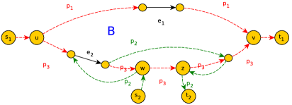
Figure 4: Illustrating why $P_{2}\neq P$ in general in Proposition 3

We would like to use the following construction at this point. Let $P_{2}$ be the path $P$ resulting from the discussion in the previous paragraph and let $e_{2}$ be the first edge on $P$ that lies in $B$. Then let $P_{3}$ be an $s_{1}\mbox{--}t_{1}$ path through $e_{2}$. Recall that $e_{2}$ lies in $H_{1}$. Now let $P_{1}$ be an $s_{1}\mbox{--}t_{1}$ path that goes through $H_{2}$ and let $e_{1}$ be an arbitrary edge on $P_{1}$ in $B$. The intention is to force the $s_{1}\mbox{--}t_{1}$ flow to use just paths $P_{1}$ and $P_{3}$, while the $s_{2}\mbox{--}t_{2}$ flow uses just path $P_{2}$, at the same time ensuring that diversity is harmful as in Proposition 2. Consider the following edge functions. $e_{1}$ and $e_{2}$ receive the same edge functions as in Proposition 2. The other edges all receive a 0 deviation. For their latency functions, edges on $P_{1}$ and $P_{3}$ that are in $B$ receive 0 functions. Outedges from $P_{1}$ and $P_{3}$ that lie in $B$ all receive functions of constant value $N$ even if they are on $P_{2}$. All as yet unassigned edges on $P_{2}$ receive 0 functions, and the remaining edges are all given functions of constant value $M\gg N$. However, the example in Figure 0.A.1 shows that there is a zero cost $s_{2}\mbox{--}t_{2}$ path ($s_{2},w,z,t_{2}$), which defeats the construction.

We fix this problem by defining the path $P_{2}$ as follows. Let $x$ be the first vertex on path $P$ (in the example, this is $w$) such that there is an edge $(x,y)$ in $B$ and such that there is a $y\mbox{--}t_{2}$ path $P_{y\mbox{--}t_{2}}$ which does not go through any ealier vertex on $P$ (i.e. any vertex from $s_{2}$ to $x$ inclusive). Then $(x,y)$ is chosen to be $e_{2}$, and $P_{2}$ is defined to be the simple path comprising the initial portion of $P$ up to $x$, followed by $e_{2}$, followed by $P_{y\mbox{--}t_{2}}$ (it may be that $P_{2}=P$). Now the above cost functions, modulo a few details, will achieve the desired contradiction. These details follow.

Let path $P_{2}$ be the simple $s_{2}\mbox{--}t_{2}$ path that follows $P$ up to $w$ and keeps following it after $w$ until for the first time it finds an edge of $B$ (and hence of $H_{1}$) that departs from a vertex of $P$ and can lead to $t_{2}$ via a path $P^{\prime}$ without returning to any of the previously visited vertices. Choose $e_{2}$ to be this edge and have $P_{2}$ follow $e_{2}$ and then path $P^{\prime}$ to $t_{2}$. Note that $P$ itself can be $P_{2}$. Consider an arbitrary $s_{1}\mbox{--}t_{1}$ simple path $P_{3}$ that goes through $e_{2}$ (and thus through $H_{1}$) and an arbitrary $s_{1}\mbox{--}t_{1}$ simple path $P_{1}$ that goes through $H_{2}$, and let $e_{1}$ be any edge of $P_{1}$ in $H_{2}$. These paths and edges are going to mimic the ones of Proposition 2. By using some large values $N$ and $M$ as latency functions for some of the edges, at both equilibria, we will ensure that all the flow of $G_{1}$ goes through the subpaths of $P_{1}$ and $P_{3}$ in $B$, and all the flow of $G_{2}$ goes through the subpath of $P_{2}$ that starts at $s_{2}$ and ends with $e_{2}$.

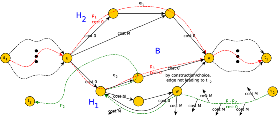
Figure 5: Sample network for Proposition 3

Let $d_{1}=d_{2}=1$ be the total demands for Commodities $1$ and $2$ respectively, and let all other commodities have $0$ demand. Let $G_{1}$’s demand consist of $\tfrac{3}{4}$ single-minded players and $\tfrac{1}{4}$ players with diversity parameter equal to $4$, and let the demand of $G_{2}$ consist of players with diversity parameter equal to $1$. Assign edge $e_{1}$ the constant latency function $\ell_{1}(x)=1$ and the constant deviation function $\sigma_{1}(x)=2$. Assign edge $e_{2}$ the constant deviation $\sigma_{2}=0$, and as latency function any $\ell_{2}$ that is continuous and strictly increasing with $\ell_{2}(1)=3$ and $\ell_{2}(\frac{5}{4})=9$. Assign all other edges the constant deviation $\sigma_{2}=0$. Assign to all other edges of $P_{1}$ and $P_{3}$ that lie inside $B$ $0$ latency functions. To all edges that depart from a vertex of $P_{1}$ or $P_{3}$ and that lie on $P_{2}$, assign latency functions equal to some big constant $N$, say $N=24$ (i.e. double the heterogeneous equilibrium cost of Proposition 2). For all remaining edges on $P_{2}$, assign $0$ latency functions. Finally, to all remaining edges, assign constant latency functions equal to $M$, where $M$ is defined to be $2|V(G)|\cdot N$.

Note that all edges other than $e_{2}$ have constant edge functions. Thus for Commodity $1$ under both equilibria there will be a common cost $C^{B^{-}}$ that will be paid on blocks other than $B$. Futhermore, for Commodity $2$, any path that costs less than $M$ will follow path $P_{2}$ up to and including $e_{2}$, for any edge leaving path $P_{2}$ either has cost $M$ or is an edge of $P_{3}$ and by construction these edges do not create a cycle-free path to $t_{2}$. Thus if any of the homogeneous or heterogeneous equilibria is to cost less than $M$ then all the flow of Commodity $2$ will go through $e_{2}$, and from there follow a least cost path to $t_{2}$ (recall all edges other than $e_{2}$ have constant edge functions) with cost $C^{e_{2}^{-}}$ say. Note that $C^{e_{2}^{-}}$ will not be more than the cost of path $P_{2}$ following edge $e_{2}$, which is bounded by $|V(G)|N=\frac{M}{2}$, and thus the path portion with cost $C^{e_{2}^{-}}$ is preferable to any path with an edge of cost $M$.

For the heterogeneous equilibrium $g$ of this instance, for Commodity $1$ route all the flow through the shortest $s_{1}\mbox{--}u$ and $v\mbox{--}t_{1}$ paths, and inside $B$ route $\tfrac{3}{4}$ units of flow through $P_{1}$ and $\tfrac{1}{4}$ units of flow through $P_{2}$, and route all the flow of commodity $2$ through $e_{2}$, via $P_{2}$ up to $e_{2}$, and after $e_{2}$ via a least cost path to $t_{2}$. The single-minded players of $G_{1}$ compute a cost for $P_{1}$ equal to $1+C^{B^{-}}$ and a cost for $P_{3}$ equal to $9+C^{B^{-}}$, and thus prefer $P_{1}$ to $P_{3}$, while the remaining players of $G_{1}$ compute a cost equal to $9+C^{B^{-}}$ for both $P_{1}$ and $P_{3}$, and thus prefer $P_{3}$ to $P_{1}$ (recall that $\ell_{2}$ is strictly increasing). The other paths have cost at least $N+C^{B^{-}}=24+C^{B^{-}}$ and thus are not preferred by any type of players. The players of Commodity $2$ pay cost equal to $9+C^{e_{2}^{-}}$ (the cost of $e_{2}$ plus the cost after it) and thus prefer staying on $e_{2}$ rather than paying at least $M$ to avoid it (recall $C^{e_{2}^{-}}\leq\frac{M}{2}$). Note that on $P_{2}$ for the vertices before $e_{2}$ there might be edges leaving $P_{2}$ that cost $0$ (these are edges of $P_{3}$) but by the definition of $P_{2}$ they cannot lead to $t_{2}$ without visiting preceding vertices. Putting it all together, this routing is indeed the heterogeneous equilibrium with cost $C^{ht}(g)=1\cdot\tfrac{3}{4}d_{1}+9\cdot\tfrac{1}{4}d_{1}+d_{1}C^{B^{-}}+9d_{2}+d_{2}C^{e_{2}^{-}}=12+C^{B^{-}}+C^{e_{2}^{-}}$.

For the homogeneous equilibrium $f$ of this instance, route all the demand of $G_{1}$ through $e_{1}$, via $P_{1}$ and the shortest $s_{1}\mbox{--}u$ and $v\mbox{--}t_{1}$ paths, and route all the flow of Commodity $2$ through $e_{2}$, via $P_{2}$ up to $e_{2}$ and from there via a least cost path to $t_{2}$. The average diversity parameter for Commodity $1$’s demand equals $1$, and thus $P_{1}$ and $P_{3}$ are both computed to cost $3+C^{B^{-}}$ while all other paths cost at least $N+C^{B^{-}}=24+C^{B^{-}}$ and thus are avoided. In the same way as above, the Commodity $2$ players pay cost equal to $3+C^{e_{2}^{-}}$ (the cost of $e_{2}$ plus the cost of the path portion following $e_{2}$) and thus prefer staying on $e_{2}$ rather than paying at least $M$ to avoid it (recall $C^{e_{2}^{-}}\leq\frac{M}{2}$). Thus the cost $C^{hm}(f)$ of the homogeneous equilibrium is $C^{hm}(f)=3\cdot d_{1}+d_{1}\cdot C^{B^{-}}+3\cdot d_{2}+d_{2}\cdot C^{e_{2}^{-}}=6+C^{B^{-}}+C^{e_{2}^{-}}$. Consequently, $C^{ht}(g)>C^{hm}(f)$, as needed.

The above instance contradicts the assumption that $G$ has the property that diversity helps for all edge functions. Thus the hypothesis that $P$, after reaching $w$ (and possibly moving backward while staying in the internal portion of $H_{1}$) first traverses an edge of $H_{1}$ (departing from an internal vertex) does not hold. This was what needed for the proposition to hold.

Proposition 4

All simple $s_{2}\mbox{--}t_{2}$ paths of $G_{2}$ that share an edge with $B$ reach $u$ before any internal vertex of $B$.

Proof

Consider an arbitrary simple $s_{2}\mbox{--}t_{2}$ path $P$ that shares some edge with $B$. WLOG we may assume, again, that $P$ only visits vertices of $G_{1}$ and $s_{2}$, $t_{2}$, as we may handle subpaths of $P$ that have vertices that lie outside $G_{1}$ as edges. Let $B$ be the parallel combination of $H_{1}$ and $H_{2}$ and, assuming that the proposition does not hold, let $w$ be the first vertex of $P$ (before it reaches $u$) that belongs to the internal portion of $B$, and suppose WLOG that $w$ lies in $H_{1}$. By Lemma 3(ii) and Proposition 3, the edge of $P$ exiting $w$ cannot go toward $t_{1}$, i.e. forward, as then it would traverse an edge of $B$ for the first time that does not depart from $u$ (recall also Lemma 4(ii)). Thus, it has to go toward $s_{1}$, i.e. backward, either staying in $H_{1}$ or going back to one of the preceding blocks of $B$. If by going backward it stays in $H_{1}$ then by the same argument it has again to move backward. However, we can only repeat this process finitely often and eventually after possibly hitting some vertices of $H_{1}$ other than $w$ and after possibly visiting vertices of blocks that precede $B$, $P$ hits $u$. Note that this happens without $P$ having hit any vertex of $H_{2}$ prior to hitting $u$ (recall Lemma 4(i)). There are two cases.

The first case occurs when on traversing $P$ up to $u$, there is some edge of $B$ departing from $u$ that does not lead to $t_{2}$ without revisiting one of the previously visited vertices. Yet, since $P$ shares an edge with $B$, by Proposition 3 there is an edge of $B$ that departs from $u$ and leads to $t_{2}$ without revisiting one of the previously visited vertices. Let $e_{1}$ be the first of the above edges and $e_{2}$ be the second one. For these edges, the same contradicting instance as in Proposition 3 can be constructed. Path $P_{1}$ is an arbitrary simple $s_{1}\mbox{--}t_{1}$ path containing $e_{1}$, path $P_{3}$ is an arbitrary simple $s_{1}\mbox{--}t_{1}$ path containing $e_{2}$, and path $P_{2}$ is constructed by following $P$ up to $u$ (instead of some internal vertex of $H_{1}$ from which $e_{2}$ was departing) and from there taking $e_{2}$ and then a path that leads to $t_{2}$ without revisiting vertices. The edge function assignment will be exactly the same. Diversity hurting, and thus the contradiction, will follow in the same way as in Proposition 3.

The second and more interesting case occurs when on following $P$ up to $u$, all edges of $B$ departing from $u$ can lead to $t_{2}$ without revisiting one of the previously visited vertices. Let $e_{2}$ be an edge of $H_{2}$ (departing from $u$) with this property, let $P_{2}$ be the simple path that follows $P$ up to $u$ and then follows some path through $e_{2}$ to go to $t_{2}$, and let $P_{3}$ be a simple $s_{1}\mbox{--}t_{1}$ path that follows an arbitrary $s_{1}\mbox{--}u$ path and an arbitrary $v\mbox{--}s_{2}$ path, and between $u$ and $v$ follows a path that contains $e_{2}$. Let $P_{1}$ be any path that follows an arbitrary $s_{1}\mbox{--}u$ path and an arbitrary $v\mbox{--}t_{2}$ path, and between $u$ and $v$ follows a path that contains $w$, and therefore goes through $H_{1}$. Let $e_{1}$ be the edge of $P_{1}$ that departs from $w$. Note that, because of Proposition 3, $e_{1}$ cannot lead to $t_{2}$ with a simple path, i.e. without visiting vertices on $P$ before $w$. This is a key fact for the contradiction to come and relates to the extra caution needed for this proof in comparison with the proof of Proposition 3. See Figure 6 for a high level description of the instance. The rest of the details can be found in the appendix, Section 0.A.6.

APPENDIX

Appendix 0.A Ommited proofs

0.A.1 An instance without average-respecting demand where diversity hurts

Let $\ell$ be any strictly increasing function with $\ell(1)=2$ and $\ell(10/9)=10$. Let there be two commodities, each of unit demand. The first commodity has demand that consists of homogeneous players with parameter equal to $10$. The second commodity has demand that consists of 1/9 players with parameter equal to $9$ and $8/9$ players with parameter equal to $0$. The heterogeneous equilibrium has cost equal to $12$ (only single-minded players are routed through the lower edge) while the homogeneous equilibrium has cost equal to $4$ (the first commodity uses only the upper edge and the second uses only the lower edge).

0.A.2 The proof of Lemma 1

The proof is by induction on the decomposition of the series-parallel network. The base case of $G$ being a single edge $e$ is trivial as $x_{e}=d_{1}\geq d_{2}=y_{e}$.

For the inductive step, first suppose that $G$ is a series combination of two series-parallel networks $G_{1}$ and $G_{2}$. For $i=1,2$, let $x^{i}$ be the restriction of flow $x$ to $G^{i}$, and $y^{i}$ the restriction of flow $y$. By the inductive hypothesis, there is an $s\mbox{--}t$ path $P_{i}$ in $G_{i}$ such that for all $e\in P_{i},x^{i}_{e}\geq y^{i}_{e}$. It suffices to set $P$ to be the concatenation of $P_{1}$ with $P_{2}$.

Now assume that $G$ is a parallel combination of two series-parallel networks $G_{1}$ and $G_{2}$. Again, for $i=1,2$, let $x^{i}$ be the restriction of flow $x$ to $G^{i}$, and $y^{i}$ of flow $y$. We may assume WLOG that the flow $d_{1}^{1}$ that $G_{1}$ receives in $x^{1}$ is at least as large as the flow $d_{2}^{1}$ that it receives in $y^{1}$, and further that $d_{1}^{1}>0$. By the inductive hypothesis applied to $G_{1}$ with demands $d_{1}^{1}$ and $d_{2}^{1}$, we obtain that there exists an $s\mbox{--}t$ path $P$ such that for all $e\in P,x^{1}_{e}\geq y^{1}_{e}$ and this implies that for all $e\in P,x_{e}\geq y_{e}$, as needed.

0.A.3 The proof of Theorem 3.2

If $G$ is not series-parallel then the Braess graph can be embedded in it (see e.g. Milchtaich [2006] or Valdes et al. [1979]). Thus, starting from the Braess network $G_{B}$, by subdividing edges, adding edges and extending one of the terminals by one edge, we can obtain $G$. Fix such a sequence of operations. For the given heterogeneous demand, we start from the Braess instance given by Proposition 1 and apply the sequence of operations one by one. Each time an edge addition occurs, we give the new edge a constant latency function equal to some large $M$ and deviation equal to $0$, each time an extension of the terminal occurs we give the new edge a constant latency and deviation equal to $0$, while each time an edge division occurs, if it is an edge with latency function $M$ we give both edges latency function equal to $M$ and deviation equal to $0$, otherwise we give one of the two edges the latency and the deviation functions of the edge that got divided and we give the other one a constant latency and deviation equal to $0$.

It is not hard to see that taking $M=2(3+\bar{r})$, i.e. more than double the heterogeneous cost of the instance of Proposition 1, (or $M=2(3A+\bar{r})$ if we must only use affine functions), suffices to ensure that all edges having latency $M$ and deviation $0$ receive zero flow in both the heterogeneous equilibrium $g$ and the homogeneous equilibrium $f$. In more detail, the only $s\mbox{--}t$ routes that may have cost $<M$ are those that starting from $s$ reach, with zero cost, some $s^{\prime}$ that corresponds to the $s$ of the instance of Proposition 1, follow some path that corresponds to one of the upper, zig-zag, or lower paths of the instance of Proposition 1, with corresponding cost, reach some $t^{\prime}$ that corresponds to $t$ of the instance of Proposition 1 and from there reach $t$ with zero cost. This can be formally proved by induction on the number of embedding steps. Thus, $C^{ht}(g)>C^{hm}(f)$ can be derived in the same way as in Proposition 1 and that is enough to prove the theorem.

0.A.4 The proof of Lemma 3

For (i), if there were such an edge then a simple $s_{i}\mbox{--}t_{i}$ path would be created that avoids the separators that lie between $B_{1}$ and $B_{2}$, contradicting the definition of $G_{i}$’s block structure.

For (ii), let $u$ and $v$ be two vertices in $G_{i}$ such that there is no simple $s_{i}\mbox{--}t_{i}$ path in $G_{i}$ that contains both of them. This implies that there is no edge between them in $G_{i}$. Now, in the series-parallel decomposition of $G_{i}$, let $B$ be the smallest series-parallel subnetwork containing both $u$ and $v$. By the choice of being smallest and the fact that there is no edge in $G_{i}$ between $u$ and $v$, $B$ must be a composition of a $B_{1}$ containing $u$ and a $B_{2}$ containing $v$. $B_{1}$ and $B_{2}$ are not connected in series because then there would be an $s_{i}\mbox{--}t_{i}$ path in $G_{i}$ containing both $u$ and $v$. Therefore, $B_{1}$ and $B_{2}$ are connected in parallel; thus there cannot be any edge in $G$ between $u$ and $v$ or else it would belong in some simple $s_{i}\mbox{--}t_{i}$ path and therefore belong to $G_{i}$, violating $G_{i}$’s series-parallel structure.

0.A.5 The proof of Lemma 4

The proofs of (i) and (ii) are by induction on the length of path $u\mbox{--}w$.

For (i), if the path has length equal to $1$ then it is a simple edge, i.e. edge $(u,w)$, and thus $u=v_{k-1}$, because of Lemma 3(i), and then (i) holds.

Now suppose inductively that the result holds for paths of length up to $l-1$. Let $u\mbox{--}w$ be a path of length $l$. Let $(u,x)$ be the first edge on this path. Note that by Lemma 3(i), $x$ cannot belong to any successor of $B_{k}$ (unless $u=v_{k-1}$ and $x=v_{k}$, in which case (i) would hold). If $x$ belongs to $B_{k}$ and is not $v_{k-1}$, then by Lemma 3(i), $u=v_{k-1}$ and thus (i) holds. If $x=v_{k-1}$ or $x$ does not belong to $B_{k}$ (which implies it belongs to a predecessor of $B_{k}$) then the inductive hypothesis holds for the length $l-1$ path $x\mbox{--}w$, yielding the desired edge exiting $v_{k-1}$. Thus (i) also holds for path $u\mbox{--}w$.

For (ii), if the path has length equal to $1$ then it is a single edge, i.e. edge $(w,u)$, and thus by Lemma 3(i)$u=v_{k}$, and (ii) holds. Now suppose inductively that the result holds for paths of length up to $l-1$. Let $w\mbox{--}u$ be a path of length $l$. Let $(w,x)$ be the first edge on this path. Either $x=v_{k}$ or $x$ is an internal vertex in $B_{k}$, by Lemma 3(i). If $x=v_{k}$ then (ii) holds. If $x$ is an internal vertex in $B_{k}$, then the inductive hypothesis applies t the length $l-1$ path $x\mbox{--}w$. Thus t(ii) also holds for path $u\mbox{--}w$.

(iii) follows from (i) and (ii). Consider an arbitrary simple $v_{k-1}\mbox{--}v_{k}$ path $P$. Path $P$ does not contain a vertex from any preceding block, for if it did, then to re-enter $B_{k}$ so as to reach $w$, according to (i), it would go through $v_{k-1}$ again, and then it would not be a simple path. Also, aside its endpoints, $P$ does not contain a vertex from any succeeding block, for if it did, then to leave $B_{k}$, according to (ii), it would reach $v_{k}$ before reaching it again at the end, and then it would not be a simple path. Thus, a path that follows some simple $s_{i}\mbox{--}v_{k-1}$ path, then follows $P$ and then follows some simple $v_{k}\mbox{--}t_{i}$ path is a simple $s_{i}\mbox{--}t_{i}$ path. Consequently, $P$ lies entirely in $B_{k}$.

0.A.6 The complete proof of Proposition 4

Consider an arbitrary simple $s_{2}\mbox{--}t_{2}$ path $P$ that shares some edge with $B$. WLOG we may assume, again, that $P$ only visits vertices of $G_{1}$ and $s_{2}$, $t_{2}$, as we may handle subpaths of $P$ that have vertices that lie outside $G_{1}$ as edges. Let $B$ be the parallel combination of $H_{1}$ and $H_{2}$ and, assuming that the proposition does not hold, let $w$ be the first vertex of $P$ (before it reaches $u$) that belongs to the internal portion of $B$, and suppose WLOG that $w$ lies in $H_{1}$. By Lemma 3(ii) and Proposition 3, the edge of $P$ exiting $w$ cannot go toward $t_{1}$, i.e. forward, as then it would traverse an edge of $B$ for the first time that does not depart form $u$ (recall also Lemma 4(ii)). Thus, it has to go toward $s_{1}$, i.e. backward, either staying in $H_{1}$ or going back to one of the preceding blocks of $B$. If by going backward it stays in $H_{1}$ then by the same argument it has again to move backward. However, we can only repeat this process finitely often and eventually after possibly hitting some vertices of $H_{1}$ other than $w$ and after possibly visiting vertices of blocks that precede $B$, $P$ hits $u$. Note that this happens without $P$ having hit any vertex of $H_{2}$ prior to hitting $u$ (recall Lemma 4(i)). There are two cases.

The first case occurs when on traversing $P$ up to $u$, there is some edge of $B$ departing from $u$ that does not lead to $t_{2}$ without revisiting one of the previously visited vertices. Yet, since $P$ shares an edge with $B$, by Proposition 3 there is an edge of $B$ that departs from $u$ and leads to $t_{2}$ without revisiting one of the previously visited vertices. Let $e_{1}$ be the first of the above edges and $e_{2}$ be the second one. For these edges, the same contradicting instance as in Proposition 3 can be constructed. Path $P_{1}$ is an arbitrary simple $s_{1}\mbox{--}t_{1}$ path containing $e_{1}$, path $P_{3}$ is an arbitrary simple $s_{1}\mbox{--}t_{1}$ path containing $e_{2}$, and path $P_{2}$ is constructed by following $P$ up to $u$ (instead of some internal vertex of $H_{1}$ from which $e_{2}$ was departing) and from there taking $e_{2}$ and then a path that leads to $t_{2}$ without revisiting vertices. The edge function assignment will be exactly the same. Diversity hurting, and thus the contradiction, will follow in the same way as in Proposition 3.

The second and more interesting case occurs when on following $P$ up to $u$, all edges of $B$ departing from $u$ can lead to $t_{2}$ without revisiting one of the previously visited vertices. Let $e_{2}$ be an edge of $H_{2}$ (departing from $u$) with this property, let $P_{2}$ be the simple path that follows $P$ up to $u$ and then follows some path through $e_{2}$ to go to $t_{2}$, and let $P_{3}$ be a simple $s_{1}\mbox{--}t_{1}$ path that follows an arbitrary $s_{1}\mbox{--}u$ path and an arbitrary $v\mbox{--}s_{2}$ path, and between $u$ and $v$ follows a path that contains $e_{2}$. Let $P_{1}$ be any path that follows an arbitrary $s_{1}\mbox{--}u$ path and an arbitrary $v\mbox{--}t_{2}$ path, and between $u$ and $v$ follows a path that contains $w$, and therefore goes through $H_{1}$. Let $e_{1}$ be the edge of $P_{1}$ that departs from $w$. Note that, because of Proposition 3, $e_{1}$ cannot lead to $t_{2}$ with a simple path, i.e. without visiting vertices on $P$ before $w$. This is a key fact for the contradiction to come. See Figure 6.

To create the instance we proceed as in Proposition 3. Let $d_{1}=d_{2}=1$ be the total demands for Commodities $1$ and $2$ respectively and let all other commodities have $0$ demand. Let $G_{1}$’s demand consist of $\tfrac{3}{4}$ single-minded players and $\tfrac{1}{4}$ players with diversity parameter equal to $4$, and let the demand of $G_{2}$ consist of players with diversity parameter equal to $1$. Assign edge $e_{1}$ the constant latency function $\ell_{1}(x)=1$ and the constant deviation function $\sigma_{1}(x)=2$. Assign edge $e_{2}$ the constant deviation $\sigma_{2}=0$, and as latency function any $\ell_{2}$ that is continuous and strictly increasing with $\ell_{2}(1)=3$ and $\ell_{2}(\frac{5}{4})=9$. Assign all other edges the constant deviation $\sigma_{2}=0$. To all other edges of $P_{1}$ and $P_{3}$ that lie inside $B$ assign $0$ latency functions. To all edges that depart from a vertex of $P_{1}$ or $P_{3}$ that lies on $P_{2}$ assign latency functions equal to some big constant $N$, say $N=24$ (i.e. double the heterogeneous equilibrium cost of Proposition 2). For all remaining edges on $P_{2}$, assign $0$ latency functions. Finally, to all remaining edges, assign constant latency functions equal to $M$, where $M$ is defined to be $2|V(G)|\cdot N$.

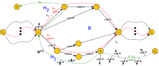
Figure 6: Sample network for Proposition 4

Note that (as in Proposition 3) all edges other than $e_{2}$ have constant edge functions. Thus for both equilibria, Commodity $1$ will have a common cost $C^{B^{-}}$ that will be paid on blocks other than $B$. Also, for Commodity $2$, any path that costs less than $M$ will follow path $P_{2}$ up to and including $e_{2}$. For this, it suffices to show that all edges departing from vertices of $P_{1}$ in between $u$ and $w$ have cost $M$, as then if some portion of the flow, after visiting $u$, deviates and follows $P_{1}$ instead of $e_{2}$, then in order to avoid edges of cost $M$ it will reach $w$ which (as mentioned earlier) would be a dead end because of Proposition 3. This is proved in the next paragraph. Given that, if both the homogeneous and the heterogeneous equilibria are to cost less than $M$ then all of Commodity $2$’s flow will go through $e_{2}$ and from there follow a shortest path to $t_{2}$ (recall that all other edges have constant edge functions) of cost $C^{e_{2}^{-}}$ say. Now note that $C^{e_{2}^{-}}$ will not be more than the cost of path $P_{2}$ following edge $e_{2}$, which is bounded by $|V(G)|N=\frac{M}{2}$, and thus the path portion with cost $C^{e_{2}^{-}}$ is preferable to any path with an edge of cost $M$.

Let $E_{M}$ be the set of edges that depart from vertices of $P_{1}$ in between $u$ and $w$. We want to prove that edges in $E_{M}$ have cost $M$. By proposition 3, the vertices of $P$ that belong to $P_{1}$ in between $w$ and $u$, $w$ included, have no departing edge that belongs to $B$ and leads to $t_{2}$ without traversing preceding vertices of $P$. This implies that $P$ and any other simple $s_{2}\mbox{--}t_{2}$ path that follows $P$ up to $u$, cannot have some simple $u\mbox{--}v$ path of $H_{2}$ as a subpath — call this Property $X$ — otherwise, by letting $P^{\prime}$ be such a path, following $P$ up to $w$, then picking any path inside $H_{1}$ that leads to $v$, and from there reaching $t_{2}$ via $P^{\prime}$, creates a simple $s_{2}\mbox{--}t_{2}$ path that has its first edge in $B$ departing from an internal vertex, thereby contradicting Proposition 3. But if $P_{2}$ is to contain some edge in $E_{M}$ then it has to leave $H_{2}$ and go to $H_{1}$. The only way to do that and keep its simplicity, because of Lemmas 3(ii) and 4(i), is by going to a block that succeeds $B$ and then coming back to $H_{1}$. But by Lemma 4(ii), going to a block that succeeds $B$ requires going through $v$ first. Thus $P_{2}$ would have a complete $u\mbox{--}v$ subpath that does not visit any other block, which by Lemma 4(iii) belongs in $B$ and thus in $H_{2}$, contradicting Property $X$. Thus $P_{2}$ does not contain any edge in $E_{M}$.

Now, we compute the costs of the equilibria The heterogeneous equilibrium $g$, for Commodity $1$, routes all the flow through the shortest $s_{1}\mbox{--}u$ and $v\mbox{--}t_{1}$ paths, inside $B$ routes $\tfrac{3}{4}$ units of flow through $P_{1}$, and $\tfrac{1}{4}$ units of flow through $P_{2}$, and routes all the flow of Commodity $2$ through $e_{2}$, via $P_{2}$ up to $e_{2}$ and after $e_{2}$ via the shortest path to $t_{2}$. The single-minded players of $G_{1}$ compute a cost for $P_{1}$ equal to $1+C^{B^{-}}$ and a cost for $P_{3}$ equal to $9+C^{B^{-}}$, and thus prefer $P_{1}$ to $P_{3}$, while the remaining players of $G_{1}$ compute a cost equal to $9+C^{B^{-}}$ for both $P_{1}$ and $P_{3}$, and thus prefer $P_{3}$ to $P_{1}$ (recall that $\ell_{2}$ is strictly increasing). The other paths have cost at least $N+C^{B^{-}}=24+C^{B^{-}}$ and thus are not preferred by any type of player. The players of Commodity $2$ pay cost equal to $9+C^{e_{2}^{-}}$ (the cost of $e_{2}$ plus the cost after it) and thus prefer staying on $e_{2}$ rather than paying at least $M$ to avoid $e_{2}$ (recall $C^{e_{2}^{-}}\leq\frac{M}{2}$). Also recall that on $P_{2}$, for the vertices before $e_{2}$, there might be edges leaving $P_{2}$ that have cost $0$ (these are edges of $P_{1}$), but because of Proposition 3 they cannot lead to $t_{2}$ without visiting preceding vertices. Putting it all together this routing is indeed the heterogeneous equilibrium with cost $C^{ht}(g)=1\cdot\tfrac{3}{4}d_{1}+9\cdot\tfrac{1}{4}d_{1}+d_{1}C^{B^{-}}+9d_{2}+d_{2}C^{e_{2}^{-}}=12+C^{B^{-}}+C^{e_{2}^{-}}$.

The homogeneous equilibrium $f$ routes all the demand of $G_{1}$ through $e_{1}$, via $P_{1}$ and the shortest $s_{1}\mbox{--}u$ and $v\mbox{--}t_{1}$ paths, and routes all the flow of Commodity $2$ through $e_{2}$, via $P_{2}$ up to $e_{2}$, and after $e_{2}$ via the shortest path to $t_{2}$. The average diversity parameter for Commodity $1$’s demand equals $1$, and thus $P_{1}$ and $P_{3}$ are both computed to cost $3+C^{B^{-}}$, while all other paths cost at least $N+C^{B^{-}}=24+C^{B^{-}}$ and thus are avoided. In the same way as above, the players of Commodity $2$ pay cost equal to $3+C^{e_{2}^{-}}$ (the cost of $e_{2}$ plus the cost after it) and thus prefer staying on $e_{2}$ rather than paying at least $M$ to avoid it. Thus the cost $C^{hm}(f)$ of the homogeneous equilibrium is $C^{hm}(f)=3\cdot d_{1}+d_{1}\cdot C^{B^{-}}+3\cdot d_{2}+d_{2}\cdot C^{e_{2}^{-}}=6+C^{B^{-}}+C^{e_{2}^{-}}$. Consequently, $C^{ht}(g)>C^{hm}(f)$, contradicting the assumption that $G$ satisfies that under any demand and edge functions diversity helps. Consequently, the proposition holds. ∎

References

- Acemoglu et al. [2016] D. Acemoglu, A. Makhdoumi, A. Malekian, and A. E. Ozdaglar. Informational braess’ paradox: The effect of information on traffic congestion. CoRR, abs/1601.02039, 2016.
- Beckmann et al. [1956] M. Beckmann, C. B. McGuire, and C. B. Winsten. Studies in the economics of transportation. Yale University Press, 1956.
- Chastain et al. [2013] E. Chastain, A. Livnat, C. H. Papadimitriou, and U. V. Vazirani. Multiplicative updates in coordination games and the theory of evolution. In ITCS ’13, 2013.
- Chen et al. [2014] P. Chen, B. de Keijzer, D. Kempe, and G. Schaefer. Altruism and its impact on the price of anarchy. ACM Transactions on Economics and Computation, 2, 2014.
- Chen et al. [2015] X. Chen, Z. Diao, and X. Hu. Excluding braess’s paradox in nonatomic selfish routing. In SAGT ’15, 2015.
- Christodoulou et al. [2014] G. Christodoulou, Kurt Mehlhorn, and Evangelia Pyrga. Improving the price of anarchy for selfish routing via coordination mechanisms. Algorithmica, 2014.
- Cole et al. [2003] R. Cole, Y. Dodis, and T. Roughgarden. Pricing network edges for heterogeneous selfish users. In STOC ’03, 2003.
- Epstein et al. [2009] A. Epstein, M. Feldman, and Y. Mansour. Efficient graph topologies in network routing games. Games and Economic Behavior, 66, 2009.
- Fleischer et al. [2004] L. Fleischer, K. Jain, and M. Mahdian. Tolls for heterogeneous selfish users in multicommodity networks and generalized congestion games. FOCS ’04, 2004.
- Fleischer [2005] L. Fleischer. Linear tolls suffice: New bounds and algorithms for tolls in single source networks. Theoretical Computer Science, 2005.
- Fotakis and Spirakis [2008] Dimitris Fotakis and Paul G. Spirakis. Cost-balancing tolls for atomic network congestion games. Internet Mathematics, 5(4):343–363, 2008.
- Fotakis et al. [2015] D. Fotakis, D. Kalimeris, and T. Lianeas. Improving selfish routing for risk-averse players. In WINE ’15, 2015.
- Karakostas and Kolliopoulos [2004a] G. Karakostas and S. G. Kolliopoulos. The efficiency of optimal taxes. In CAAN ’04, 2004.
- Karakostas and Kolliopoulos [2004b] G. Karakostas and S.G. Kolliopoulos. Edge pricing of multicommodity networks for heterogeneous selfish users. FOCS ’04, 2004.
- Kleer and Schäfer [2016] P. Kleer and G. Schäfer. The impact of worst-case deviations in non-atomic network routing games. In SAGT ’16, pages 129–140, 2016.
- Lianeas et al. [2016] T. Lianeas, E. Nikolova, and N. E. Stier-Moses. Asymptotically tight bounds for inefficiency in risk-averse selfish routing. In IJCAI ’16, 2016.
- Mehta et al. [2015] R. Mehta, I. Panageas, and G. Piliouras. Natural selection as an inhibitor of genetic diversity: Multiplicative weights updates algorithm and a conjecture of haploid genetics [working paper abstract]. In ITCS ’15, 2015.
- Meir and Parkes [2014] R. Meir and D. C. Parkes. Playing the wrong game: Bounding externalities in diverse populations of agents. CoRR, abs/1411.1751, 2014. To appear in AAMAS ’18.
- Milchtaich [2006] I. Milchtaich. Network topology and the efficiency of equilibrium. Games and Economic Behavior, 57, 2006.
- Nikolova and Stier-Moses [2014] E. Nikolova and N. E. Stier-Moses. A mean-risk model for the traffic assignment problem with stochastic travel times. Operations Research, 62, 2014.
- Nikolova and Stier-Moses [2015] E. Nikolova and N. E. Stier-Moses. The burden of risk aversion in mean-risk selfish routing. In EC ’15, 2015.
- Piliouras et al. [2013] G. Piliouras, E. Nikolova, and J. S. Shamma. Risk sensitivity of price of anarchy under uncertainty. In EC ’13, 2013.
- Rockafellar [2007] R.T. Rockafellar. Coherent approaches to risk in optimization under uncertainty. Tutorials in Op. Research, 2007.
- Schmeidler [1973] D. Schmeidler. Equilibrium points of nonatomic games. Journal of Statistical Physics, 7, 1973.
- Valdes et al. [1979] J. Valdes, R. E. Tarjan, and E. L. Lawler. The recognition of series parallel digraphs. In STOC ’79, 1979.