Generalized Knudsen Number for Unsteady Fluid Flow

Abstract

We explore the scaling behavior of an unsteady flow that is generated by an oscillating body of finite size in a gas. If the gas is gradually rarefied, the Navier-Stokes equations begin to fail and a kinetic description of the flow becomes more appropriate. The failure of the Navier-Stokes equations can be thought to take place via two different physical mechanisms: either the continuum hypothesis breaks down as a result of a finite size effect; or local equilibrium is violated due to the high rate of strain. By independently tuning the relevant linear dimension and the frequency of the oscillating body, we can experimentally observe these two different physical mechanisms. All the experimental data, however, can be collapsed using a single dimensionless scaling parameter that combines the relevant linear dimension and the frequency of the body. This proposed Knudsen number for an unsteady flow is rooted in a fundamental symmetry principle, namely Galilean invariance.

The Navier-Stokes (NS) equations of hydrodynamics can be obtained perturbatively from the kinetic theory of gases in the limit of small Knudsen number, ${\rm Kn}=\frac{\lambda}{\cal L}\to 0$ Landau_Physical_Kinetics . Here, $\lambda$ is the mean free path in the gas, and $\cal L$ represents a characteristic length scale of the flow. As ${\rm Kn}\to 0$, it follows from statistical mechanics that density fluctuations in the gas vanish Huang , leading to the notion of a “fluid particle.” This continuum hypothesis becomes less accurate as $\rm Kn$ grows, eventually leading to the failure of the NS equations for $\rm Kn\gtrsim 0.1$. Likewise, the NS equations break down if the local value of the strain rate, $S_{ij}=\frac{1}{2}\left(\frac{\partial u_{i}}{\partial x_{j}}+\frac{\partial u_{j}}{\partial x_{i}}\right)$, becomes so large that the condition $\tau S_{ij}\ll 1$ no longer holds. Here, $u_{i}$ represents the velocity vector, and $\tau$ is the relaxation time that characterizes the rate of decay of a perturbation to thermodynamic equilibrium. As $\tau S_{ij}$ grows, the fluid particle becomes deformed on shorter and shorter time scales, eventually violating the local equilibrium assumption. For a broad class of flows, breakdown of the continuum hypothesis and violation of local equilibrium can be thought to be equivalent, because $\tau S_{ij}\sim\tau\frac{U}{\cal L}\sim\frac{\lambda}{c}\frac{U}{\cal L}\sim\rm Ma\times Kn$. Here, the Mach number ${\rm Ma}=\frac{U}{c}$ compares the speed of sound $c$ to the characteristic flow velocity $U$, and it is assumed to remain small and slowly varying. Thus, either $\rm Kn$ or $\tau S_{ij}$ emerges as the relevant scaling parameter for determining the crossover from hydrodynamics to kinetic theory.

To demonstrate the limitations of the above-described widely-accepted reasoning, we consider the canonical problem of an infinite plate oscillating at a ${\it prescribed}$ angular frequency $\omega_{0}$ in a gas (Stokes Second Problem) Landau_Fluids . We assume the oscillation amplitude to be small and the geometry to be such that the velocity field is $u_{x}(x,y,0)=U_{0}{\cos\omega_{0}t}$, $u_{y}=0$, and $u_{z}=0$. Since the plate is infinite ($l\to\infty$), the “standard” size-based Knudsen number ${\rm Kn}_{l}=\frac{\lambda}{l}$ remains zero at all limits and cannot be relevant. The scaling parameter here is the Weissenberg number, $\rm Wi=\omega_{0}\tau$ Ekinci ; Rarefied , and one can recover the correct Knudsen number, $\rm{Kn}_{\delta}=\frac{\lambda}{\delta}$, using the boundary layer thickness, $\delta=\sqrt{\frac{2\nu_{g}}{\omega_{0}}}$. (Indeed, $\rm{Kn}_{\delta}\sim\sqrt{\rm Wi}$, given the kinematic viscosity is $\nu_{g}\sim\frac{\lambda^{2}}{\tau}$.) Regardless, $\tau S_{ij}\approx\tau\frac{U_{0}}{\delta}\sim{\rm Ma\times Kn}_{\delta}$. Thus, as above, the validity of the NS equations (and the scaling properties of the flow) is determined either by the flow length scale (${\rm Kn}_{\delta}$) or by the flow time scale ($\tau S_{ij}$ or $\rm Wi$), and both parameters lead to the same conclusion. While this analysis for an infinite plate is reasonable, it does not work for a finite plate (or a finite-sized body). For a finite-sized body, ${\rm Kn}_{l}$ may be non-zero at some limit and appear in the problem alongside $\rm Wi$. This is because the oscillation frequency $\omega_{0}$ is in general independent of the linear dimensions of the body and an externally-prescribed parameter. Recent literature on scaling of such flows reflects this complexity: some reports suggest ${\rm Kn}_{l}$ scaling Bullard ; Martin ; Bhiladvala and others $\rm Wi$ scaling Karabacak ; Ekinci ; Svitelsky . The purpose of the present work is to study this non-trivial limit and to recover, both experimentally and theoretically, the universal scaling hidden in the apparent contradictions.

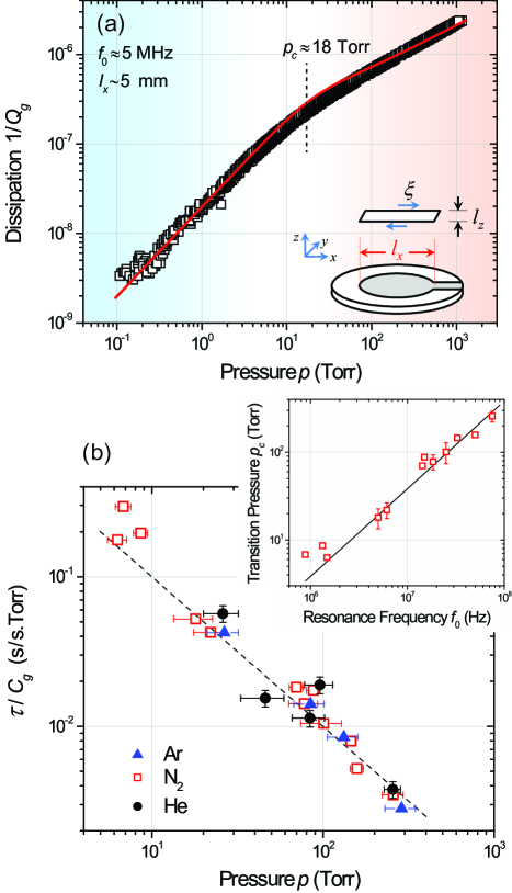
Figure 1: (a) Dissipation in N₂ as a function of pressure for a quartz crystal (inset) oscillating in shear mode at $f_{0}\approx 5$ MHz. Solid line is a fit to Eq. (1). Transition from the kinetic to viscous regime occurs at $p_{c}\approx 18$ Torr. (b) The inset shows $p_{c}$ vs. $f_{0}$ for different quartz crystals in N₂ (${\rm Kn}_{l}\approx 0$). The linear fit gives the empirical $\tau$ as a function of $p$. The main figure shows $\tau/{\cal C}_{g}$ for He, N₂, and Ar as a function of $p$. Normalization by ${\cal C}_{g}$ accounts for the differences between gases Supplemental . Dashed line is $1/p$. Error bars are not shown when smaller than symbols.

Our experimental measurements are based on quartz crystals, and micro- and nano-mechanical resonators. When driven to oscillations in a gas, these structures generate oscillatory flows and dissipate energy. The gases used are high-purity He, N₂, and Ar. The approximate equation of motion of a mechanical resonator (in any resonant mode) is that of a damped harmonic oscillator: $\ddot{\xi}+\frac{\omega_{0}}{Q_{t}}\dot{\xi}+{\omega_{0}}^{2}\xi={\cal F}(t)/m_{r}$, where $\xi(t)$ is the amplitude, $m_{r}$ is the mass, $1\over Q_{t}$ is the total (dimensionless) dissipation, and $\omega_{0}=2\pi f_{0}$ is the angular frequency of the mode driven by the sinusoidal force ${\cal F}(t)$. In a typical experiment, the pressure $p$ of the gas is changed, and $1\over Q_{t}$ and $\omega_{0}$ are measured. For all practical purposes, $\omega_{0}$ stays constant through $p$ sweeps. To obtain the (dimensionless) gas dissipation $\frac{1}{Q_{g}}$, we calculate $\frac{1}{Q_{g}}=\frac{1}{Q_{t}}-\frac{1}{Q_{0}}$, where $\frac{1}{Q_{0}}$ is the intrinsic dissipation (obtained at the lowest $p$). Relevant parameters of our resonators and other details can be found in the Supplemental Material Supplemental .

All our ${1\over Q_{g}}$ vs. $p$ data possess similar features (Figs. 1a, 2a, 3a, 3b S2-S10). At low $p$, ${1\over Q_{g}}\propto p$. This is the kinetic limit Christian ; Gombosi , where the mean free path $\lambda$ and the relaxation time $\tau$ of the gas are both large. At high $p$, the NS equations are to be used Landau_Fluids . The crossover between these two asymptotes (transitional flow regime) manifests itself as a slope change in the data. The pressure $p_{c}$, around which this transition occurs, is therefore a fundamentally important parameter and provides insight into how this flow scales. ($p_{c},\tau_{c}$ and $\lambda_{c}$ henceforth indicate transition values.)

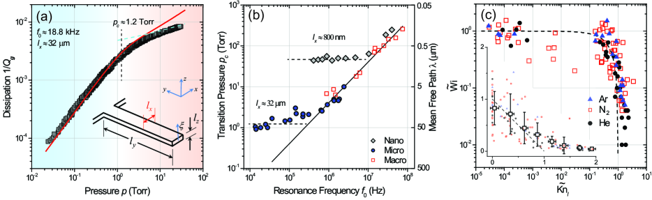
Figure 2: (a) Dissipation vs. pressure for a microcantilever (inset) with $l_{x}\times l_{y}\times l_{z}\approx 32\times 350\times 1~{}\mu\rm m^{3}$ and $f_{0}\approx 18.8$ kHz in N₂. Solid line is a fit to Eq. (4); dotted (blue) line is a fit to the cylinder solution; $p_{c}\approx 1.2$ Torr. (b) $p_{c}$ vs. $f_{0}$ in N₂ for three sets of devices with different characteristic dimensions. Diamonds are nanocantilevers from ref. Kara ; circles are microcantilevers; squares are macroscopic resonators from Fig. 1b. (c) $\tilde{\rm Wi}$ and ${\tilde{\rm Kn}}_{l}$ in He, N₂, and Ar for all devices. Dashed line is $\tilde{\rm Wi}+{\tilde{\rm Kn}}_{l}=1$. The inset shows the same data using linear axes; the large data points correspond to binned average values.

We first analyze the dissipation of a macroscopic quartz crystal resonator in shear-mode oscillations in N₂ (Fig. 1a). The resonance frequency is $f_{0}=\frac{\omega_{0}}{2\pi}\approx 5$ MHz, and the relevant linear dimension is roughly the diameter of the metal electrode on the quartz, $l_{x}\sim 5$ mm (Fig. 1a inset). For the shown pressures, ${\rm Kn}_{l}=\frac{\lambda}{l_{x}}$ is in the range $10^{-5}\lesssim{\rm Kn}_{l}\lesssim 10^{-1}$, found using $\lambda\approx\frac{{{k_{B}}T}}{{\sqrt{2}\pi{{d_{g}}^{2}}p}}$, where $k_{B}T$ is the thermal energy and $d_{g}$ is the diameter of a N₂ molecule. Because ${\rm Kn}_{l}$ remains small, we treat the quartz as an infinite plate and ${\rm Wi}=\omega_{0}\tau$ is left as the only relevant scaling parameter. The transition from molecular flow ($\omega_{0}\tau\gg 1$) to viscous flow ($\omega_{0}\tau\ll 1$) must take place at ${\tilde{\rm Wi}}=\omega_{0}\tau_{c}\approx 1$. Hence, we call this the “high-frequency limit.” Next, we perform the same $\frac{1}{Q_{g}}$ vs. $p$ measurement on similarly large quartz resonators but with different $f_{0}$. We determine $p_{c}$ consistently for all by finding the pressure at which $\frac{1}{Q_{g}}$ deviates from the low-$p$ asymptote by $25\%$. The inset of Fig. 1b shows the measured $p_{c}$ values in N₂ as a function of $f_{0}$. The data scale as ${{p_{c}}}={\rm{constant}}\times f_{0}$. This is consistent with the flow being scaled by ${\rm Wi}=\omega_{0}\tau$ and $\omega_{0}\tau_{c}\approx 1$ determining the transition: $\tau=\frac{{\cal C}_{\rm N_{2}}}{p}$ for a near-ideal gas with ${\cal C}_{\rm N_{2}}$ being a constant; $\omega_{0}\tau_{c}\approx\omega_{0}\frac{{\cal C}_{\rm N_{2}}}{p_{c}}\approx 1$, and ${p_{c}}\approx 2\pi{{\cal C}_{\rm N_{2}}}\times f_{0}$. The experiment provides the empirical value ${\cal C}_{\rm N_{2}}=610\pm 30\times 10^{-9}$ in units of s$\cdot$Torr. Repeating the same experiment for He and Ar, we find ${\cal C}_{\rm He}=560\pm 70\times 10^{-9}$ and ${\cal C}_{\rm Ar}=750\pm 80\times 10^{-9}$, both in units of s$\cdot$Torr. Figure 1b (main) is a collapse plot of $\tau/{\cal C}_{g}$ for all three gases as a function of $p$, showing the degree of linearity. The measured values of ${\cal C}_{g}$ for all gases are a factor of $\sim 5$ larger than the kinetic theory predictions Supplemental ; Reif .

The data in Fig. 1a can be fit accurately Ekinci . For a large plate resonator (${\rm Kn}_{l}\approx 0$), the dissipation in a gas of viscosity $\mu_{g}$ and density $\rho_{g}$ can be found as Yakhot_Colosqui ; Supplemental

$$\frac{1}{Q_{g}}=\frac{S_{r}}{m_{r}}f(\omega_{0}\tau)\sqrt{\frac{{\mu_{g}\rho_{g}}}{{2\omega_{0}}}}.$$ (1)

Here, $S_{r}$ is the surface area and $m_{r}$ is the mass of the plate resonator, and $f$ is the scaling function Yakhot_Colosqui found as $f(x)=\frac{1}{{(1+x^{2})^{3/4}}}\left[(1+x)\cos\left({\frac{{\tan^{-1}x}}{2}}\right)\right.\left.-(1-x)\sin\left({\frac{{\tan^{-1}x}}{2}}\right)\right]$. The fit in Fig. 1a was obtained using the empirical relation $\tau=\frac{610\rm\times 10^{-9}[s\cdot Torr]}{p}$ and experimental parameters Supplemental .

Now, we turn to the “low-frequency limit” of $\omega_{0}\tau\to 0$. Figure 2a shows the pressure-dependent dissipation of a low-frequency microcantilever with linear dimensions $l_{x}\times l_{y}\times l_{z}\approx 32\times 350\times 1~{}\mu\rm m^{3}$ (inset Fig. 2a) and frequency $f_{0}=18.8$ kHz. We define ${\rm Kn}_{l}=\frac{\lambda}{l_{x}}$, as suggested in Seo ; Mertens ; Martin . The transition in Fig. 2a takes place around $p_{c}\approx 1.2$ Torr, where ${\rm Kn}_{l}\approx 1$ and $\omega_{0}\tau\approx 0.06$. (${\rm Kn}_{l}\approx 1$ indicates deviation from the low-$p$ molecular asymptote.) The features in Fig. 2a are very similar to those in Fig. 1a: two asymptotes with a well-defined $p_{c}$. Inspection of the ranges of $\rm Wi$ and ${\rm Kn}_{l}$ suggests that the transition cannot be tied to frequency ($\rm Wi$) but must be due to the length scale (${\rm Kn}_{l}$). In other words, the transition from molecular flow (${\rm Kn}_{l}\gg 1$) to viscous flow (${\rm Kn}_{l}\ll 1$) appears to take place around ${\tilde{\rm Kn}_{l}}=\frac{\lambda_{c}}{l_{x}}\approx 1$. While the data trace in Fig. 2a looks similar to that in Fig. 1a, the transitions observed in the two are due to different physical mechanisms.

In Fig. 2b, we plot the consistently-found $p_{c}$ in N₂ for different sets of devices. Here, the relevant linear dimension $l_{x}$ is kept constant for each set, but the frequency is varied: diamond nanocantilevers Kara with $l_{x}\approx 800$ nm and $0.4~{}{\rm MHz}\leq f_{0}\leq 40~{}{\rm MHz}$; silicon microcantilevers with $l_{x}\approx 32~{}\mu\rm m$ and $14~{}{\rm kHz}\leq f_{0}\leq 2.4~{}{\rm MHz}$; and quartz crystals with $l_{x}\sim 5$ mm and $5~{}{\rm MHz}\leq f_{0}\leq 75~{}{\rm MHz}$. Surprisingly, the linear trend between $p_{c}$ and $f_{0}$ holds only for high frequencies, with a saturation at low frequencies. The saturation value of $p_{c}$ is determined by the condition that $\lambda\sim\l_{x}$ (dotted horizontal lines). The oscillation frequency (and $\rm Wi$) becomes the relevant scaling parameter above a certain frequency; at low frequency, the length scale (${\rm Kn}_{l}$) takes over. Thus, the physics is determined by an interplay between the relevant length scale of the body and its oscillation frequency.

To gain more insight into the transition, we scrutinize ${\tilde{\rm Kn}}_{l}=\frac{\lambda_{c}}{l_{x}}$ and $\tilde{\rm Wi}=\omega_{0}\tau_{c}$ for each device at its $p_{c}$. Figure 2c shows ${\tilde{\rm Kn}}_{l}$ and $\tilde{\rm Wi}$ plotted in the $xy$-plane using logarithmic and linear axes (inset); the dashed lines are $\tilde{\rm Wi}+{\tilde{\rm Kn}}_{l}=1$. The data suggest that the dissipation is a function of both ${\rm Wi}$ and ${\rm Kn}_{l}$, and it approximately depends on ${\rm Wi}+{\rm Kn}_{l}$.

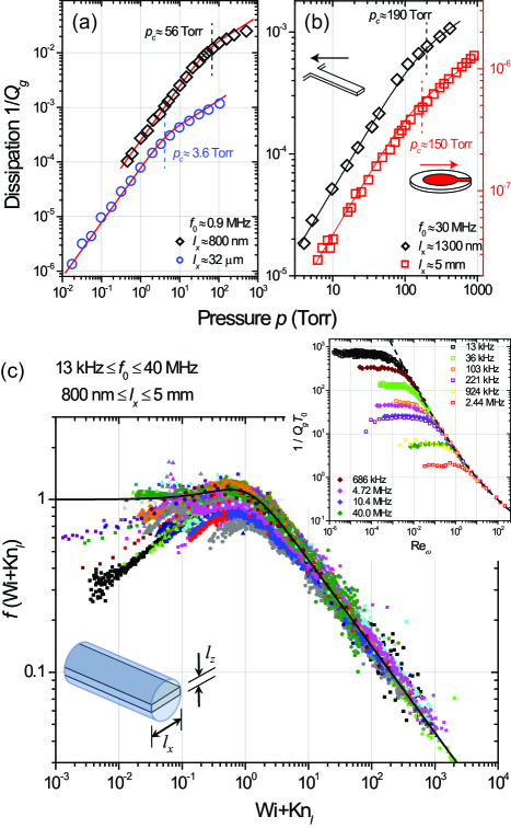
Figure 3: (a) Dissipation vs. $p$ for two cantilevers with different length scales but similar frequencies ($l_{x}\approx 800$ nm, $f_{0}\approx 894$ kHz; and $l_{x}\approx 32~{}\mu$m, $f_{0}\approx 924$ kHz) in N₂. Transitions are determined by ${\rm Kn}_{l}\approx 1$ at $p_{c}\approx 56$ Torr and 3.6 Torr, respectively. (b) Dissipation for a nanocantilever ($l_{x}\approx 1300$ nm, $f_{0}\approx 28.6$ MHz) and a macroscopic quartz crystal ($l_{x}\sim 5$ mm, $f_{0}\approx 32.7$ MHz Ekinci ); the transitions take place around 190 Torr and 150 Torr, respectively. (c) Collapse plot for all the data in different gases. The thick solid line shows the scaling function $f$. The inset is a collapse of select cantilever data based on the viscous cylinder solution. Squares and diamonds correspond to microcantilevers ($l_{x}\approx 32~{}\mu$m) and nanocantilevers ($l_{x}\approx 800$ nm), respectively. Dashed line shows the imaginary part of the complex hydrodynamic function for a cylinder. The lower inset shows the parameters of the model.

We now justify the observed scaling more rigorously by inspecting the stress tensor $\sigma_{ij}$ obtained from the Chapman-Enskog expansion of the Boltzmann equation in the relaxation time approximation. To second order of smallness, the expansion is Chen

$$\begin{split}{\sigma_{ij}}\approx{\sigma_{ij}^{(1)}}+{\sigma_{ij}^{(2)}}=&2\rho_{g}\theta\Bigl{[}\tau{S_{ij}}-\tau\left({{{\partial\over{\partial t}}}+{\bf{u}}\cdot\nabla}\right)(\tau{S_{ij}})\\ &+2{\tau^{2}}\left({{S_{ik}}{S_{kj}}-\frac{{{\delta_{ij}}}}{3}{S_{kl}}{S_{kl}}}\right)\\ &-2{\tau^{2}}\left({{S_{ik}}{\Omega_{kj}}+{S_{jk}}{\Omega_{ki}}}\right)\Bigr{]}.\end{split}$$ (2)

As usual, ${S_{ij}}=\frac{1}{2}\left({\frac{{\partial{u_{i}}}}{{\partial{x_{j}}}}+\frac{{\partial{u_{j}}}}{{\partial{x_{i}}}}}\right)$ and ${\Omega_{ij}}=\frac{1}{2}\left({\frac{{\partial{u_{i}}}}{{\partial{x_{j}}}}-\frac{{\partial{u_{j}}}}{{\partial{x_{i}}}}}\right)$ are the strain rate and the vorticity tensors, respectively, with $i,j=x,y,z$; and $\theta=\frac{k_{B}T}{m_{g}}$. The last two terms of $\sigma_{ij}$ are the second rank tensor $\xi_{ij}^{(2)}$ of order $(\tau{\bf{S}})^{2}$, where ${\bf{S}}$ represents the strain rate tensor. There are two dimensionless groups in Eq. (2): the total time derivative $\tau\frac{d}{dt}=\tau\left(\frac{\partial}{\partial t}+{\bf{u}}\cdot\nabla\right)$ and $\tau{\bf{S}}$. One notices that these two dimensionless groups both remain invariant under Galilean transformations Supplemental . In order to satisfy Galilean invariance, therefore, the Chapman-Enskog expansion of kinetic equations must be in powers of these parameters only; powers of non-Galilean-invariant parameters, e.g., “bare” $\frac{\partial}{\partial t}$, are forbidden in a flow in an arbitrary geometry. Accordingly, one can formally write the Galilean-invariant stress tensor up to all orders as

$$\begin{split}&{\sigma_{ij}}=2{\rho_{g}}\theta[\tau{S_{ij}}+\\ &\sum\limits_{n=2}^{\infty}{\left({{\alpha_{n-1}}{{(-\tau)}^{n-1}}{{\left({{\partial\over{\partial t}}+{\bf{u}}\cdot\nabla}\right)}^{n-1}}(\tau{S_{ij}})+\xi_{ij}^{(n)}}\right)}].\end{split}$$ (3)

Here, $\alpha_{n-1}$ are constants, and the tensors $\xi_{ij}^{(n)}\sim(\tau{\bf{S}})^{n}$ are not necessarily zero expansion_comment .

A closed form formula can be obtained for the dissipation of a finite-sized body oscillating in a fluid, if the deviations from the infinite plate solution Yakhot_Colosqui are assumed small. As in the infinite plate Yakhot_Colosqui ; Supplemental , we set all $\alpha_{k}\approx 1$ and all $\xi_{ij}^{(n)}\approx 0$ in Eq. (3). After non-dimensionalization with ${\bf{\hat{u}}}={{\bf{u}}\over c}$, $\hat{t}={\omega_{0}}t$ and $\hat{\nabla}={{l}\nabla}$, the stress tensor ${\sigma_{ij}}$ for a finite-sized body becomes an expansion in powers of the operator $\tau\frac{d}{dt}={{\omega_{0}}\tau{\partial\over{\partial\hat{t}}}+{\rm{K}}{{\rm{n}}_{l}}{\bf{\hat{u}}}\cdot\hat{\nabla}}$. The scaling parameter therefore becomes approximately ${\omega_{0}\tau+\rm Kn}_{l}$, and the infinite plate solution in Eq. (1) can be generalized by replacing $\omega_{0}\tau$ with $\omega_{0}\tau+{\rm Kn}_{l}$. Thus, we deduce Supplemental

$$\frac{1}{Q_{g}}\approx\frac{S_{r}}{m_{r}}f(\omega_{0}\tau+\frac{\lambda}{l_{x}})\sqrt{\frac{{\mu_{g}\rho_{g}\tau}}{{2(\omega_{0}\tau+\frac{\lambda}{l_{x}})}}}.$$ (4)

for a finite-sized body oscillating in a fluid. Several points are noteworthy. First, Eq. (4) is valid in the asymptotic and the intermediate ranges. Second, the non-dimensionalization above is eminently reasonable, because the only velocity scale in kinetic theory is the thermal velocity $\sim c$. Regardless, the dimensional solution is obtained only after imposing the boundary conditions. Finally, Galilean invariance dictates the form of $\frac{d}{dt}$ and leads to a scaling parameter $\approx{\rm Wi+Kn}_{l}$, instead of a more involved combination of ${\rm Wi}$ and ${\rm Kn}_{l}$.

A number of fits to experimental data using Eq. (4) are shown in Figs. 2a, 3a, and 3b as well as in the Supplemental Material Supplemental . The data in Fig. 3a and 3b are examples of the low- and high-frequency limits, respectively. Here, different-sized but similar-frequency resonators are compared. All fits are obtained as follows. First, $S_{r}/m_{r}$ is determined from linear dimensions or from separate measurements when necessary Supplemental . For each pressure, the value of $\omega_{0}\tau+\frac{\lambda}{l_{x}}$ is computed using $\tau={\cal C}_{g}/p$ and $\lambda\approx 0.23\frac{k_{B}T}{{d_{g}}^{2}p}$ of the gas, and $\l_{x}$ and $\omega_{0}$ of the resonator. Finally, the dissipation is found from Eq. (4) at each pressure using tabulated $\mu_{g}$ and $\rho_{g}$, and our empirical $\tau$. To improve the fits, the theoretical prediction is multiplied by an ${\cal O}(1)$ constant ${\cal Q}_{p}$ . The collapse plot in Fig. 3c is obtained by properly dividing the data by $\frac{S_{r}}{m_{r}}\sqrt{\frac{{\mu_{g}\rho_{g}\tau}}{{2(\omega_{0}\tau+\frac{\lambda}{l_{x}})}}}{\cal Q}_{p}$ and plotting the results as a function of $\omega_{0}\tau+\frac{\lambda}{l_{x}}$. The thick solid line shows $f({\rm Wi+Kn}_{l})$. There are no free parameters other than the fitting factors ${\cal Q}_{p}$ with mean $\bar{\cal Q}_{p}\approx 2.6\pm 0.5$ Supplemental .

At the viscous limit ${\rm Wi+Kn}_{l}\ll 1$, the cantilever data deviate from the plate solution and converge to a cylinder solution. The cylinder solution yields $\frac{1}{{{Q_{g}}}}\approx\frac{{{\Gamma_{I}}({\rm Re}_{\omega})}}{1/T_{0}+{{\Gamma_{R}}({\rm Re}_{\omega})}}$ Sader ; Paul . Here, $\Gamma({\rm Re}_{\omega})=\Gamma_{R}({\rm Re}_{\omega})+i\Gamma_{I}({\rm Re}_{\omega})$ is the complex hydrodynamic function for a cylinder and only depends upon the (oscillatory) Reynolds number ${\rm Re}_{\omega}=\frac{\omega_{0}{l_{x}}^{2}}{4\nu_{g}}$; $T_{0}=\frac{\pi}{4}\frac{\rho_{g}l_{x}}{\rho_{r}l_{z}}$ with $\rho_{r}$ being the density of the solid (Fig. 3c lower inset). For our gas experiments, $1/T_{0}\gtrsim 1000\gg\Gamma_{R}$, and thus $\frac{1}{{{Q_{g}T_{0}}}}\approx\Gamma_{I}({\rm Re}_{\omega})$. The upper inset of Fig. 3c shows $\frac{1}{{{Q_{g}T_{0}}}}$ from representative cantilevers with different parameters plotted against ${\rm Re}_{\omega}$; dashed line shows $\Gamma_{I}({\rm Re}_{\omega})$. In each case, a fitting constant ${\cal Q}_{c}$ with mean ${\bar{\cal Q}_{c}}\approx 0.9\pm 0.2$ is used Supplemental . The data converge to the cylinder solution in the viscous regime.

We conclude that the scaling parameter for an arbitrary time-dependent isothermal flow should be a function of both $\rm Wi$ and ${\rm Kn}_{l}$. We show that a generalized Knudsen number in the form ${\rm Wi+Kn}_{l}$ works well and can be justified by Galilean invariance.

- (1) E. M. Lifshitz and L. P. Pitaevskii, Physical Kinetics (Butterworth-Heinemann, Oxford, 1981).
- (2) K. Huang, Statistical Mechanics (New York, London, 1963).
- (3) L. D. Landau and E. M. Lifshitz, Fluid Mechanics (Butterworth-Heinemann, Oxford, 1987), 2nd ed.
- (4) K. L. Ekinci, D. M. Karabacak, and V. Yakhot, Phys. Rev. Lett. 101, 264501 (2008).
- (5) In rarefied gas dynamics, this parameter is called the “temporal Knudsen number.” See, for example, C. Shen, Rarefied Gas Dynamics: Fundamentals, Simulations and Micro Flows (Springer-Verlag, Berlin, Heidelberg, 2005) or N. G. Hadjiconstantinou, Phys. Fluids 17, 100611 (2005).
- (6) E. C. Bullard, J. Li, C. R. Lilley, P. Mulvaney, M. L. Roukes, J. E. Sader, Phys. Rev. Lett. 112, 015501 (2014).
- (7) M. J. Martin, B. H. Houston, J. W. Baldwin, and M. K. Zalalutdinov, J. MEMS 17, 503 (2008).
- (8) R. B. Bhiladvala, and Z. J. Wang, Phys. Rev. E 69, 036307 (2004).
- (9) D. M. Karabacak, V. Yakhot, and K. L. Ekinci, Phys. Rev. Lett. 98, 254505 (2007).
- (10) O. Svitelskiy, V. Sauer, N. Liu, K.-M. Cheng, E. Finley, M. R. Freeman, and W. K. Hiebert, Phys. Rev. Lett. 103, 244501 (2009).
- (11) See Supplemental Material URL for a description of methods and further data, which includes Refs. [4, 15, 16, 21-37].
- (12) R. G. Christian, Vacuum 16, 175 (1966).
- (13) T. I. Gombosi, Gaskinetic Theory (Cambridge University Press, New York, 1994).
- (14) F. Reif, Fundamentals of Statistical and Thermal Physics (McGraw-Hill, New York, 1965).
- (15) V. Kara, Y.-I. Sohn, H. Atikian, V. Yakhot, M. Loncar, and K. L. Ekinci, Nano Lett. 15, 8070 (2015).
- (16) V. Yakhot and C. Colosqui, J. Fluid Mech. 586, 249 (2007).
- (17) D. Seo, M. R. Paul, and W. A. Ducker, Rev. Sci. Instrum. 83, 055005 (2012).
- (18) J. Mertens, E. Finot, T. Thundat, A. Fabre, M. H. Nadal, V. Eyraud, and E. Bourillot, Ultramicroscopy, 97, 119 (2003).
- (19) H. Chen, S. A. Orszag, I. Staroselsky, and S. Succi, J. Fluid Mech. 519, 301 (2004).
- (20) Depending on the flow problem, the expansion may contain other terms, such as mixed powers of time and space derivatives. Such terms are omitted here for clarity.
- (21) J.E. Sader, J. W. M. Chon, P. Mulvaney, Rev. Sci. Instrum. 70, 3967 (1999).
- (22) M. R. Paul, M. T. Clark, and M. C. Cross, Phys. Rev. E 88, 043012 (2013).
- (23) C. Lissandrello, V. Yakhot, K. L. Ekinci, Phys. Rev. Lett. 108, 084501 (2012).
- (24) S. Ramanathan, D. L. Koch, R. B. Bhiladvala, Physics of Fluids 22, 103101 (2010).
- (25) M. Bao, H. Yang, H. Yin, Y. Sun, J. Micromech. Microeng 12, 341 (2002).
- (26) M. Herrscher, C. Ziegler, and D. Johannsmann, J. Appl. Phys. 101, 114909 (2007).
- (27) C. D. F. Honig, J. E. Sader, P. Mulvaney, W. A. Ducker, Phys. Rev. E 81, 056305 (2010).
- (28) C. D. F. Honig, and W. A. Ducker, J. Phys. Chem. C 114, 20114 (2010).
- (29) S. Rajauria, O. Ozsun, J. Lawall, V. Yakhot, and K. L. Ekinci, Phys. Rev. Lett. 107 174501 (2011).
- (30) D. Johannsmann, Phys. Chem. Chem. Phys. 10, 4516 (2008).
- (31) K. Kokubun, M. Hirata, H. Murakami, Y. Toda, and M. Ono, Vacuum 34, 731, (1984).
- (32) B. Borovsky, B. L. Mason, and J. Krim, J. Appl. Phys. 88, 4017 (2000).
- (33) J. F. O’Hanlon, A user’s guide to vacuum technology (John Wiley & Sons, 2005), 3rd ed.
- (34) K. L. Ekinci, V. Yakhot, S. Rajauria, C. Colosqui, and D. M. Karabacak, Lab on a Chip 10, 3013 (2010).
- (35) D. B. Vogt, K. L. Eric, W. Wu, and C. C. White, J. Phys. Chem. B 108, 12685 (2004).
- (36) T. Zhu, W. Ye, and J. Zhang, Phys. Rev. E 84, 056316 (2011); T. Zhu and W. Ye, Phys. Rev. E 82, 036308 (2010).
- (37) G. Chen, Nanoscale Energy Transport and Conversion (Oxford University Press, New York, 2005).